contrast predictor user guide - defence research...

Matlab contrast Predictor user guide

Vincent Ross Aerex Avionics Inc

Prepared By: Aerex Avionics Inc 324 St-Augustin Beakeyville Québec GOS 1E1 Contractor Report Number: 2013-125216-AT3-001 PWGSC Contract Number: W7701-125216 Technical Authority: Denis Dion, Defence Scientist, DRDC – Valcartier Research Centre.

Disclaimer: The scientific or technical validity of this Contract Report is entirely the responsibility of the Contractor and the contents do not necessarily have the approval or endorsement of the Department of National Defence of Canada.

Contract Report DRDC-RDDC-2016-C148 October 2013

© Her Majesty the Queen in Right of Canada, as represented by the Minister of National Defence, 2016.

© Sa Majesté la Reine (en droit du Canada), telle que représentée par le ministre de la Défense nationale, 2016.

324, Ave St-Augustin, Breakeyville (Québec), Canada, G0S IE1 telephone: (4I8) 832-I040, fax: (4I8) 832-9831, e-mail: [email protected]

AEREX Report No: 2013-125216-AT3-001

Matlab contrast Predictor user guide

Submitted to

Denis Dion DRDC Valcartier

2459, Boulevard Pie-XI North Québec (Québec) Canada, G3J 1X5

in the framework of contract number

W7701-125216-AT3/001/QCL

Authored by:

Vincent Ross

The scientific or technical validity of this Contract Report is entirely the responsibility of the Contractor and the contents do not necessarily have the approval or endorsement of the Department of National Defence of Canada.

This document was reviewed for Controlled Goods by DRDC Valcartier

October 2013

intentionally left blank.

Sa majesté la reine du Canada, représentée par le ministre de la Défense nationale, 2015 Her Majesty the Queen, as represented by the Minister of National Defence, 2015

MatLab contrast Predictor user guide

AEREX Report Number: 2013-125216-AT3-001

Version: 1.0 The scientific or technical validity of this Contract Report is entirely the responsibility of the contractor and the contents do not necessarily have the approval or endorsement of Defence R&D Canada. L’entrepreneur est seul responsable de la validité scientifique ou technique de ce rapport de contrat et son contenu n’a pas nécessairement reçu l’approbation ou l’appui de R et D pour la défense Canada.

Author: (Original signed by) 15 October 2013 Vincent Ross (date) Physicist Publication reviewed by: (Original signed by) 15 October 2013 Paul Lacasse, ing. MBA (date) Senior Project Manager Publication approved by: (Original signed by) 15 October 2013 Daniel Pomerleau, Eng. (date) President, AEREX inc.

Abstract ……..

This document is the user guide for a tool called Contrast Predictor designed to calculate the contrast of a target against its background from the visible to the thermal infrared bands (0.4 to 13 microns). The model includes heating of the target by the environment during the diurnal cycle and considers environmental and meteorological parametrization. This tool was developed by AEREX Avionics inc. under contract W7701-125216-AT3/001/QCL for DRDC-Valcartier between September 6th 2012 and September 6th 2013.

Résumé ….....

Ce document est le guide usager pour un outil appelé Predicteur de Contraste conçu pour calculer le contraste d’une cible sur son l’arrière-plan du visible à l’infrarouge thermique (de 0.4 à 13 microns). Le modèle inclue le réchauffement de la cible par l’environnement durant le cycle diurnal et considère la paramétrisation environnemental et météorologique. Cet outil a été développé par AEREX Avionique inc. Sous le contrat W7701-125216-AT3/001/QCL pour le RDDC-Valcartier entre le 6 Septembre 2012 et le 6 Septembre 2013.

AEREX Report Number: 2013-125216-AT3-001 i

This page intentionally left blank.

ii AEREX Report Number: 2013-125216-AT3-001

Executive summary

Contrast Predictor user guide: Vincent Ross; AEREX Report Number: 2013-125216-AT3-001, AEREX Avionics Inc; October 2013

Introduction or background: The atmosphere plays many roles that affect the detection of a target of interest in a spectrally band integrated image. It is therefore important to properly model the atmosphere both radiatively and thermally in its interaction with the target and background in order to predict the appearance of both entities and calculate the radiative contrast between them. The contrast can then be used as a criterion for the possibility of target detection.

Results: Under contract W7701-125216-AT3/001/QCL, AEREX Avionics Inc. developed a tool for Defence Research and Development Canada Valcartier to evaluate the effect of atmospheric conditions, target composition and geometry and background nature on the target to background contrast. The tool is named Contrast Predictor. In this document, we describe the use of that tool.

Significance: This tool can be used to design reconnaissance missions more effectively by predicting periods in a diurnal cycle when contrast between the target and background disappears, a phenomenon called thermal crossover. It can also become an effective tool to verify the effectiveness of newly designed sensors.

Future plans: A new interface written in the C++ coding language is being developed with the same functionalities but a more streamlined interface. Features will be added as needs arise.

AEREX Report Number: 2013-125216-AT3-001 iii

Sommaire .....

Contrast Predictor user guide: Vincent Ross; AEREX Report Number: 2013-125216-AT3-001, AEREX Avionics Inc; October 2013

Introduction ou contexte : L’Atmosphère joue plusieurs rôles qui affectent la détection d’une cible d’intérêt dans des images en bandes larges. Il est donc important de modéliser correctement l’atmosphère autant sur le plan radiatif que thermique dans son interaction avec la cible et son arrière-plan dans le but de prédire leur apparence et de calculer le contraste radiatif entre eux. Le contraste peut alors être utilisé comme critère de possibilité de détection.

Résultats : Sous le contrat W7701-125216-AT3/001/QCL, AEREX Avionics Inc. a développé un outil pour Recherche et Développement pour la Défense du Canada à Valcartier pour évaluer l’effet des conditions atmosphériques, de la composition et de la géométrie de la cible ainsi que de la nature de l’arrière-plan sur le contraste radiatif entre la cible et l’arrière-plan. Cet outil se nomme Prédicteur de Contraste. Ce document décrit l’utilisation de cet outil.

Importance : Cet outil peut être utilisé pour mettre en place des missions de reconnaissance de façon plus efficace en prédisant les périodes dans le cycle diurnal quand le contraste entre la cible et l’arrière-plan devient nul un phénomène qui se nomme l’inversion de contraste thermique. L’outil pourra aussi être utilisé pour vérifier l’efficacité de nouveaux détecteurs.

Perspectives : Une nouvelle interface graphique écrit dans le langage de programmation C++ est en développement avec les mêmes fonctionnalités mais avec un interfaçage plus dynamique. De nouvelles fonctionnalités seront ajoutées au besoin.

iv AEREX Report Number: 2013-125216-AT3-001

Table of contents

Contrast Predictor user guide ........................................................................................................... i Abstract …….. ................................................................................................................................. i Résumé …..... ................................................................................................................................... i Executive summary ........................................................................................................................ iii Sommaire ..... .................................................................................................................................. iv Table of contents ............................................................................................................................. v List of figures ................................................................................................................................ vii Acknowledgements ........................................................................................................................ ix 1 Introduction ............................................................................................................................... 1 2 Installation and requirements .................................................................................................... 2 3 Starting Contrast Predictor........................................................................................................ 3 4 Navigating from one panel to the other .................................................................................... 4 5 Configurations .......................................................................................................................... 5

5.1 Configuring MODTRAN .............................................................................................. 5 5.2 Configuring Environment Canada forecast (optional) .................................................. 6 5.3 Configure Display preferences ...................................................................................... 7

6 Scene pannel ............................................................................................................................. 9 6.1 Sensor Parameters ......................................................................................................... 9 6.2 Scene parameters ......................................................................................................... 10 6.3 Terrain parameters ....................................................................................................... 10 6.4 Scene visualization ...................................................................................................... 11

7 Atmosphere pannel ................................................................................................................. 13 7.1 Atmosphere type .......................................................................................................... 13 7.2 Radiative fluxes ........................................................................................................... 14 7.3 Aerosols ....................................................................................................................... 15 7.4 Viewing temporal profiles ........................................................................................... 17 7.5 Building a user defined atmosphere ............................................................................ 18

8 Target panel ............................................................................................................................ 22 8.1 Target properties and position .................................................................................... 22 8.2 Target orientation ........................................................................................................ 23 8.3 Building a custom target .............................................................................................. 24

8.3.1 Specifying the top and bottom properties .......................................................... 26 8.3.2 Target internal structure ..................................................................................... 28

9 Results panel ........................................................................................................................... 31 10 Additional information ........................................................................................................... 35 References ..... ............................................................................................................................... 36

AEREX Report Number: 2013-125216-AT3-001 v

List of symbols/abbreviations/acronyms/initialisms ..................................................................... 37 Distribution list .............................................................................................................................. 38

vi AEREX Report Number: 2013-125216-AT3-001

List of figures

Figure 1: Contrast Predictor immediately after start-up on the surface parameter screen............... 3

Figure 2: Progress bar ...................................................................................................................... 4

Figure 3: MODTRAN setup menu .................................................................................................. 5

Figure 4: MODTRAN configuration dialog. ................................................................................... 5

Figure 5: Forecast menu .................................................................................................................. 6

Figure 6: Environment Canada Forecast Configuration dialog. ...................................................... 7

Figure 7: Display menu. .................................................................................................................. 7

Figure 8: Display preferences configuration dialog ........................................................................ 8

Figure 9: Sensor parameters on the Scene pane .............................................................................. 9

Figure 10: Scene parameter set on the Scene pane. ....................................................................... 10

Figure 11: Terrain parameter set on the Scene pane...................................................................... 11

Figure 12: Scene configuration display on the scene pane. ........................................................... 12

Figure 13: Atmosphere pane. ........................................................................................................ 13

Figure 14: Atmosphere type parameters ........................................................................................ 14

Figure 15: Radiative fluxes parameters ......................................................................................... 14

Figure 16: Aerosol model selection ............................................................................................... 16

Figure 17: Atmospheric profile display ......................................................................................... 17

Figure 18: Atmosphere builder screen........................................................................................... 18

Figure 19: Temporal surface data group on the Atmosphere Builder interface. ........................... 20

Figure 20: Target parameter panel................................................................................................. 22

Figure 21: Target properties parameter group ............................................................................... 23

Figure 22: Target orientation parameter group .............................................................................. 24

Figure 23: Target builder window ................................................................................................. 24

Figure 24: Target Builder configuration when Ambient Temperature (left) and Constant Temperature (right) are selected. ................................................................................ 25

Figure 25: Target Boundary Definition screen .............................................................................. 26

Figure 26: Parameters group on the Target Boundary Definition screen for a constant temperature boundary (left) and for a constant flux boundary (right). ........................ 27

Figure 27: Parameters group on the Target Boundary Definition screen for a free surface when Single Albedo (left) and Dual Albedo (right) is selected. ................................. 28

Figure 28: Internal target material structure interface. .................................................................. 28

AEREX Report Number: 2013-125216-AT3-001 vii

Figure 29: Target Layer Definition window. ................................................................................. 29

Figure 30: Results panel in contrast view ...................................................................................... 31

Figure 31: Results panel in target temperature view ..................................................................... 32

Figure 32: Fixed Sensor contrast map example. ............................................................................ 33

Figure 33: Fixed target contrast map example .............................................................................. 33

viii AEREX Report Number: 2013-125216-AT3-001

Acknowledgements

The author would like to thank Mr. Paul Lacasse for his thorough review and useful comments and insight regarding the production of this document.

AEREX Report Number: 2013-125216-AT3-001 ix


x AEREX Report Number: 2013-125216-AT3-001

1 Introduction

The atmosphere plays many roles that affect the detection of a target of interest in a spectrally band integrated image. It absorbs and scatters light in and out of the optical path from the target to the sensor affecting the overall target signal, and does the same to the background behind the target reducing the target contrast. The atmosphere also has a role in the intrinsic appearance of the target. Its radiance reflects off the target and background surfaces affecting their appearances. Finally, the atmosphere affects the temperature of the target and background depending on the meteorological conditions. It is therefore important to properly model the atmosphere both radiatively and thermally in its interaction with the target and background in order to predict the appearance of both entities and calculate the radiative contrast between them. The contrast can then be used as a criterion for the possibility of target detection. Under contract W7701-125216/001/QCL [1], AEREX Avionics Inc. developed a tool for Defence Research and Development Canada Valcartier to evaluate the effect of atmospheric conditions, target composition and geometry and background nature on the target to background contrast. The tool is named Contrast Predictor. In this document, we describe the use of that tool. It can be used to design reconnaissance missions more effectively by predicting periods in a diurnal cycle when contrast between the target and background disappears, a phenomenon called thermal crossover. It can also become an effective tool to verify the effectiveness of newly designed sensors.

AEREX Report Number: 2013-125216-AT3-001 1

2 Installation and requirements

The Contrast Predictor is based on the EOSPEC library. It is therefore necessary to install the EOSPEC library on you system and configure all path variables correctly. The distribution of the Contrast Predictor comes with precompiled dlls required to interface the Matlab [2] Java environment. If your system is not set up to compile these, you will need to copy them onto your system. Note: is a newer version of EOSPEC exists on your computer, this will revert the EOSPEC dlls to an earlier version. If you wish to keep the newer version on your system, adjust the path variables to point to the dlls distributed with the Contrast Predictor. Steps for installation are:

1) Copy the contents of the /bin directory in you EOSPEC bin directory.

2) Make sure your EOSPEC_DIR environment variable points to the root of the EOSPEC installation

3) Put the full path to the EOSPEC /bin directory on you user PATH environment variable.

4) Configure the Matlab librarypath.txt file (You probably need admin privileges to modify this file!)

Open C:/Program Files (x86)/MATLAB/R2009b/toolbox/local/librarypath.txt

Note: replace R2009b by your version of Matlab

Add EOSPEC dll directory at end of file. For example, if the EOSPEC dll directory is:

C:/Users/vross/Documents/svn_code/eospec/bin/vs2008

the librarypath.txt file looks like this: ## ## FILE: librarypath.txt ## ## Entries: ## o path_to_jnifile ## o [alpha,glnx86,sol2,unix,win32,mac]=path_to_jnifile ## o $matlabroot/path_to_jnifile ## o $jre_home/path_to_jnifile ## $matlabroot/bin/$arch C:/Users/vross/Documents/svn_code/eospec/bin/vs2008

5) Restart Matlab 32 bit

NOTE: steps 1) trough 3) only need to be executed once. The Contrast Predictor will only work with a Windows 32 bit version of Matlab.

2 AEREX Report Number: 2013-125216-AT3-001

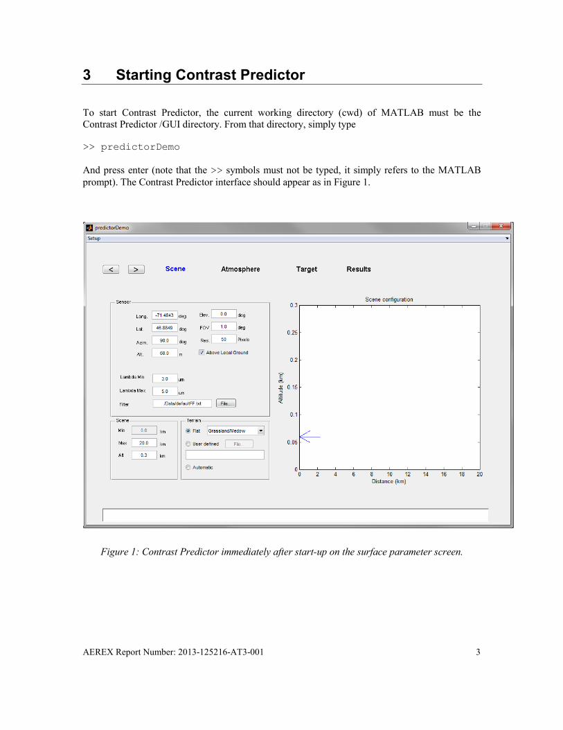
3 Starting Contrast Predictor

To start Contrast Predictor, the current working directory (cwd) of MATLAB must be the Contrast Predictor /GUI directory. From that directory, simply type

>> predictorDemo

And press enter (note that the >> symbols must not be typed, it simply refers to the MATLAB prompt). The Contrast Predictor interface should appear as in Figure 1.

Figure 1: Contrast Predictor immediately after start-up on the surface parameter screen.


4 Navigating from one panel to the other

It is strongly suggested you fill out the scene pane parameters before proceeding to other panes. In fact, on the first pass through the GUI, all panes should be filled out completely in order. This is because some parameters and displays in further panels have dependencies on prior panels. Because of this, the application is set up as a “wizard”. To navigate from one panel to the other, use the button to go forward, and use the button to go back. If you change something in a previous panel, all calculations are invalidated and need to be redone when moving forward again. Note that while going forward, you may have to wait a few seconds for calculations to occur. A progress bar at the bottom of the screen indicates calculation progress (Figure 2).

Figure 2: Progress bar


5 Configurations

5.1 Configuring MODTRAN

Contrast Predictor uses the MODTRAN® (versions 4.3.1) [2] software in order to function. The first step is to configure the location of the MODTRAN directories as well as some version related information. Configuration will be necessary only for the first use of Contrast Predictor, or if your MODTRAN installation changes directory. To configure, simply select the Setup -> Modtran menu (Figure 3), or use the Ctrl+M keyboard shortcut. This opens the MODTRAN configuration dialog (Figure 4).

Figure 3: MODTRAN setup menu

Figure 4: MODTRAN configuration dialog.


MODTRAN Path: This is the path to the MODTRAN console executable. The MODTRAN executable should be located at the root directory level of the MODTRAN installation. You can type in the full path to the MODTRAN console executable or browse to its location by using the Browse… button.

I/O Directory: This is the directory where all MODTRAN input and output files will be saved. MODTRAN usually has a TEST directory that can be used for this purpose, but you can specify any other directory of your choosing. You can type in the full path to the directory or browse to its location by using the Browse… button.

Case name: This is the name that will be given to all MODTRAN input and output files. For example, if the case name is test_case, the modtran input file will be named test_case.tp5 as for MODTRAN’s naming convention.

Spectral Database Version: Disabled in the current version of the Predictor.

Once all appropriate MODTRAN information has been entered, click “Ok” to accept the configuration or “Cancel” to discard changes.

5.2 Configuring Environment Canada forecast (optional)

If you wish to use Environment Canada meteorological predictions in the contrast calculation, you need to configure the location of the forecast data on your computer (note that the data is not retrieved by the application). To do this, select Setup -> Forecast or use the Ctrl+F keybord shortcut (Figure 5). This opens the Forecast configuration dialog (Figure 6). You can enter the full path to the Environment Canada GRIB files is the provided field, or use the “Browse...” button to browse to the directory.

Figure 5: Forecast menu


Figure 6: Environment Canada Forecast Configuration dialog.

5.3 Configure Display preferences

You can choose how the application displays certain quantities such as the time. To do so, simply select Setup -> Display (Figure 7) to open the display configuration dialog (Figure 8). From this dialog, you can choose to display times as UTC. If UTC time is unchecked, you need to specify the time zone to display, and select if daylight savings time is to be calculated. By default, the application automatically selects the proper time zone and daylight savings from your current computer settings.

Figure 7: Display menu.


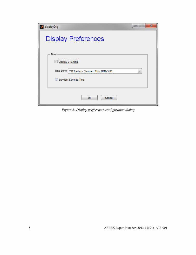
Figure 8: Display preferences configuration dialog


6 Scene pannel

The first set of parameters to provide is located on the “Scene” pane (Figure 1).

6.1 Sensor Parameters

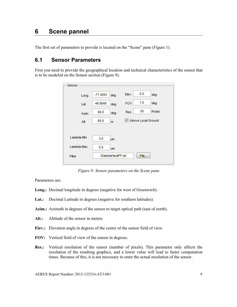
First you need to provide the geographical location and technical characteristics of the sensor that is to be modeled on the Sensor section (Figure 9).

Figure 9: Sensor parameters on the Scene pane

Parameters are:

Long.: Decimal longitude in degrees (negative for west of Greenwich).

Lat.: Decimal Latitude in degrees (negative for southern latitudes).

Azim.: Azimuth in degrees of the sensor to target optical path (east of north).

Alt.: Altitude of the sensor in meters

Elev.: Elevation angle in degrees of the center of the sensor field of view.

FOV: Vertical field of view of the sensor in degrees.

Res.: Vertical resolution of the sensor (number of pixels). This parameter only affects the resolution of the resulting graphics, and a lower value will lead to faster computation times. Because of this, it is not necessary to enter the actual resolution of the sensor.


Above local ground: If checkbox is enabled, the reference point for the sensor altitude is the ground at the sensor coordinates; otherwise it is the mean sea level.

Lambda Min.: Minimum wavelength of the sensor band in microns.

Lambda Max.: Maximum wavelength of the sensor band in microns.

Filter: Path to the file containing the sensor response (filter) function. The file should be an ASCII file with an arbitrary length comment header (preceded by # symbols) and two number columns for the wavelength and filter function respectively. For example:

#Triangular Filter Function #Wavelength Function #(micron) (normalized) 3.0 0.0 4.0 1.0 5.0 0.0

You can type the path in the provided field, or use the button to navigate to the file.

6.2 Scene parameters

The scene parameter set on the scene pane relate to the scene extent (Figure 10). The parameters are:

Min.: Disabled in the current version

Max.: The maximum extent of the scene in kilometers.

Alt.: The scene cut-off altitude in kilometers above mean sea level.

Figure 10: Scene parameter set on the Scene pane.

6.3 Terrain parameters

The terrain parameter set (Figure 11) on the scene panel specifies the terrain altitude profile in the direction of the sensor azimuth. There are three different ways to specify the terrain:


• Flat: The terrain is perfectly flat and uniform at 0 km above sea level. The reflective properties of the terrain are specified by a selection of surface composition from the drop-down list (see Figure 11).

• User defined: The vertical terrain profile is specified by a user defined file. The path to the file can by typed directly in the provided field, or you can use the button to navigate to the file. An example terrain file is provided in the /Data directory (example.ter).

• Automatic: A digital terrain elevation database (DTED) and a coverage database are used to calculate the terrain profile and surface coverage automatically. In the current version, only a small database spanning longitudes from -71.5o to -71 o and latitudes from 46.75o to 47o is provided. Elevation data is from www.geobase.ca/geobase/en/data/cded/index.html while terrain coverage is from http://tree.pfc.forestry.ca/nts_prov.html.

Figure 11: Terrain parameter set on the Scene pane.

6.4 Scene visualization

As parameters are provided, it is possible to visualize to scene in the scene configuration display (Figure 12). The terrain profile is depicted as well as the sensor position, altitude, elevation and field of view. The sensor looks something like an inverted arrow. The center line represents the center of the field of view look direction, while the lower and upper lines represent the span of the field of view. Note that since the scene horizontal extent is often much larger than the vertical extent, depicted objects usually have a heavily distorted aspect ratio.


http://www.geobase.ca/geobase/en/data/cded/index.html

http://tree.pfc.forestry.ca/nts_prov.html

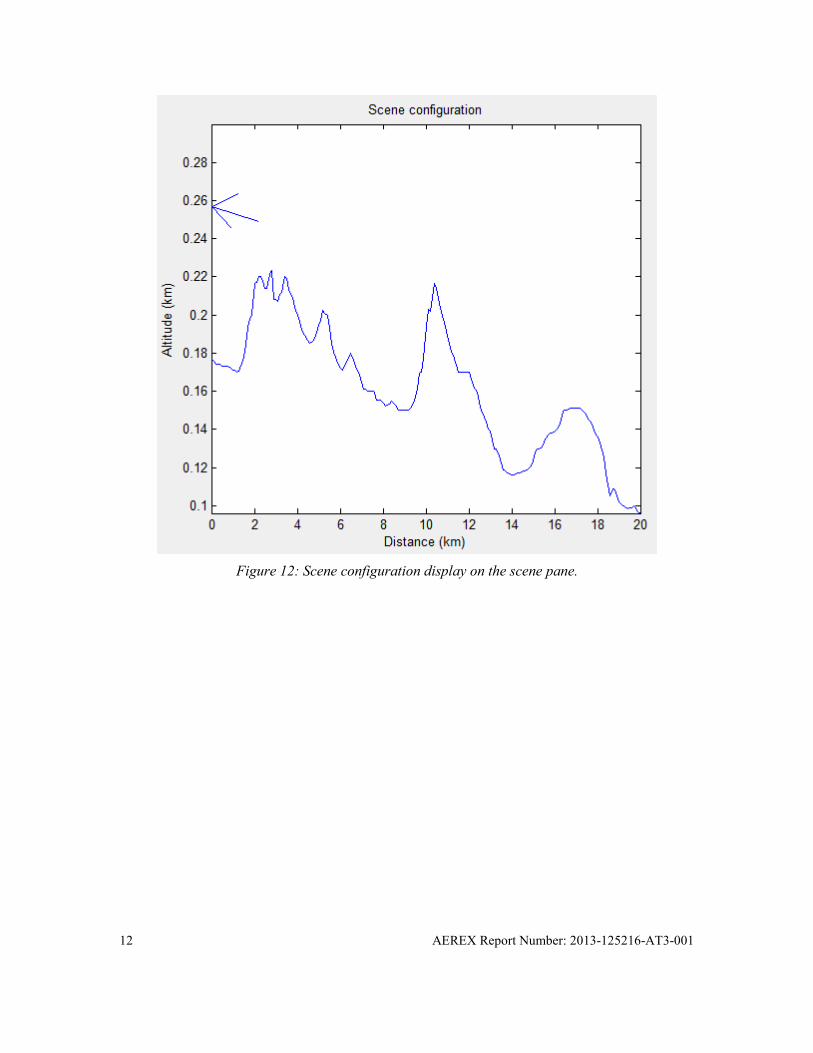
Figure 12: Scene configuration display on the scene pane.


7 Atmosphere pannel

The next step is to enter parameters to describe the atmosphere thermodynamic and radiative properties on the atmosphere pane (Figure 13).

Figure 13: Atmosphere pane.

7.1 Atmosphere type

The type of atmosphere input must be selected. Choices are:

• User defined: You can define the temporal variations of the atmosphere using the “Define…” button (see section 7.5) or you can load a predefined atmosphere (.atm file) by using the “Load…” button.

• Forecast: If the Environment Canada forecast data directory is properly configured (see section 5.2), you can select this option. Enter the date of the forecast (provided in case multiple forcasts exist on your computer) in dd/mm/yyyy format and press the “Load Environment Canada Forecast” button.


Figure 14: Atmosphere type parameters

7.2 Radiative fluxes

Radiative fluxes affect how target and background appear from surface reflections, and have an important role in target heating and cooling. There are different ways to specify radiative fluxes (Figure 15):

Prediction: Disabled in the current version.

SMARTI Calculations: Calculate radiative fluxes using the SMARTI radiative transfer code. Note that selecting this option can lead to slow calculations.

Empirical: Uses a fast empirical relation to estimate fluxes.

Ground measurements: Lets you load surface measurements from a meteorological station using the button. An example file 14_07-18_10_2011_Meteo_table1.dat is provided.

Figure 15: Radiative fluxes parameters


7.3 Aerosols

The aerosol parameter set lets you choose and control the boundary aerosol model used in the simulation (Figure 16). Choices are:

• None: No boundary aerosols are used;

• Rural: Best for rural conditions, 23 km visibility;

• NAM: Navy aerosol model, for maritime environments, visibility set according to wind speed;

• Maritime: for maritime environments, fixed 23 km extinction;

• Urban: best for urban environments, 5 km visibility;

• Tropospheric: background boundary aerosols with 50 km visibility;

• Advective fog: 0.2 km default visibility; and

• Radiative fog: 0.5 km default visibility.

•

With some selection (NAM and DRDC Maritime) additional parameters can become available (Figure 16 on the right):

AMP: Air mass parameter (also called air mass character or ICSTL in MODTRAN), defines the continental influence (from 1 to 10).

Fetch: The distance (km) over which the wind has traveled since leaving the coast. Available for the DRDC Maritime model only.


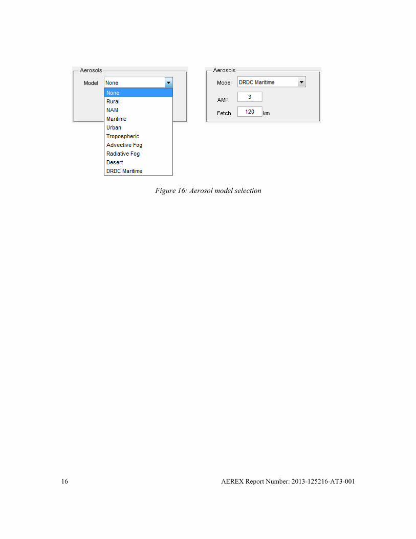
Figure 16: Aerosol model selection


7.4 Viewing temporal profiles

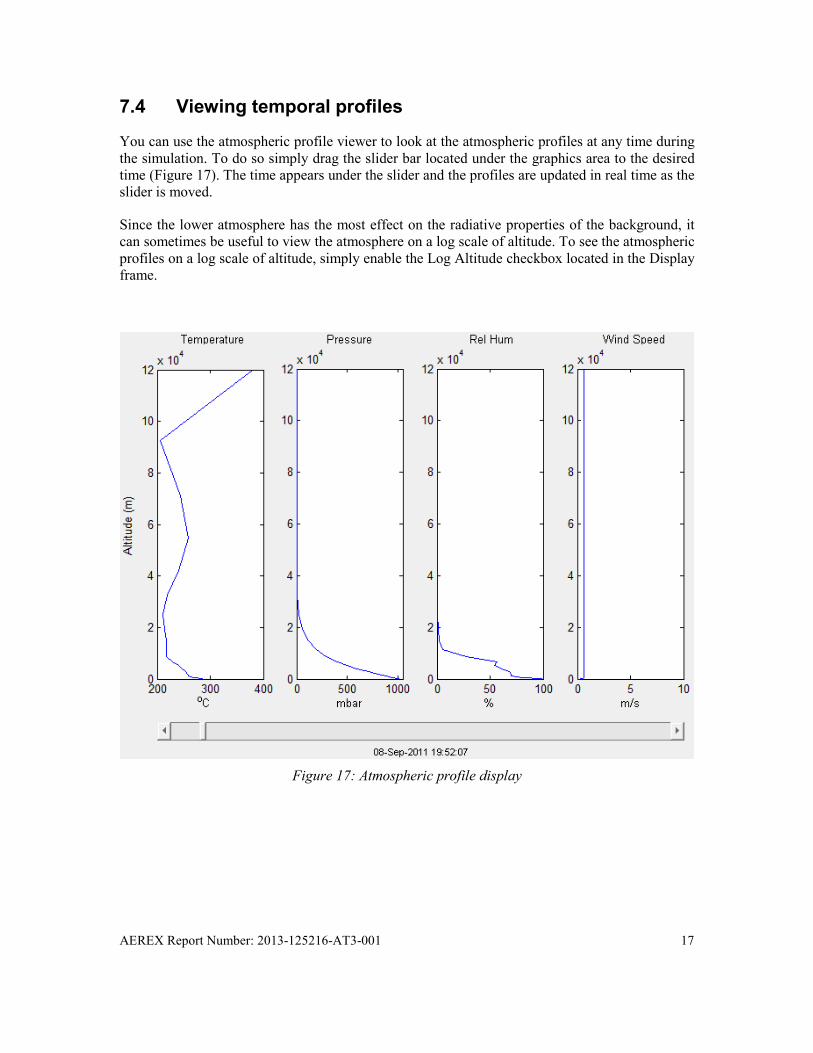
You can use the atmospheric profile viewer to look at the atmospheric profiles at any time during the simulation. To do so simply drag the slider bar located under the graphics area to the desired time (Figure 17). The time appears under the slider and the profiles are updated in real time as the slider is moved.

Since the lower atmosphere has the most effect on the radiative properties of the background, it can sometimes be useful to view the atmosphere on a log scale of altitude. To see the atmospheric profiles on a log scale of altitude, simply enable the Log Altitude checkbox located in the Display frame.

Figure 17: Atmospheric profile display


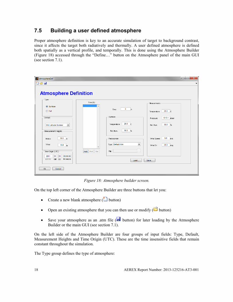
7.5 Building a user defined atmosphere

Proper atmosphere definition is key to an accurate simulation of target to background contrast, since it affects the target both radiatively and thermally. A user defined atmosphere is defined both spatially as a vertical profile, and temporally. This is done using the Atmosphere Builder (Figure 18) accessed through the “Define…” button on the Atmosphere panel of the main GUI (see section 7.1).

Figure 18: Atmosphere builder screen.

On the top left corner of the Atmosphere Builder are three buttons that let you:

• Create a new blank atmosphere ( button)

• Open an existing atmosphere that you can then use or modify ( button)

• Save your atmosphere as an .atm file ( button) for later loading by the Atmosphere Builder or the main GUI (see section 7.1).

On the left side of the Atmosphere Builder are four groups of input fields: Type, Default, Measurement Heights and Time Origin (UTC). These are the time insensitive fields that remain constant throughout the simulation.

The Type group defines the type of atmosphere:


Surface: Only surface measurements, and possibly radiosonde measurements vary with time, while most of the atmosphere remains constant.

Full: The atmosphere is fully defined at each time step. This option is NOT supported in the current version. Selecting this option results in an error.

The Default frame contains a drop down list where you can select the atmosphere profile to use for altitudes not covered by the temporal profiles. The atmospheres are:

• US Standard 1976;

• Midlatitude Summer;

• Midlatitude Winter;

• Subarctic Summer;

• Subarctic Winter; and

• Tropical.

The Measurement Heights group define at what height (meters) the meteorological station sensors are located for wind and meteo (temperature, pressure, relative humidity). This has an impact on the shape of the profile in the lower boundary layer.

Finally, the Time Origin (UTC) group sets the origin (zero time) of the simulation. All user defined time varying quantities are defined according to a time offset to the origin. As the group name implies, the time origin must be UTC.

When the atmosphere type is “Surface” (the only supported option in the current version), the right side of the Atmosphere Builder shows the temporal surface data (Figure 19). This group features a list of all time offset (in decimal hours) for which surface data is entered. By clicking on a list item you can display the surface data for the selected time offset to the right of the list. On Figure 19 for example, the 1.2 h offset data is displayed. Below the list are three buttons:

Add: After entering new surface data in the fields on the right, press this button to add the record to the temporal surface data. The “Time” field must not already exist.

Mod: If you modify any field on the right for a selected time offset record, you need to press this button to save the new values to the record. Simply changing the values does not reflect permanently on the record.

Del: This button deletes the selected record, and the time offset is removed from the list.


Figure 19: Temporal surface data group on the Atmosphere Builder interface.

To the right of the list is located a series of fields and field groups reflecting the surface data for a particular time offset:

Time: The time offset from the time origin in decimal hours

The “Surface” group contains fields defining air properties just above the ground:

Temperature: The temperature of the air just above the ground (usually the same as the ground temperature) in degrees Celsius.

Rel. Hum.: The relative humidity of the air just above the ground in percent.

The “Radiosonde” group defines the atmosphere above the lower surface boundary layer (about the first 30 meters):

Type: a drop down list letting you select the type of radiosonde file to use. Choises are:

• Default Atm: Use the default atmosphere entered in the “Default” drop down list on the left for all atmospheric levels above the lower surface boundary layer.

• Temp: Use a TEMP format radiosonde file. The TempFmt0inversion.rs, TempFmt1inversion.rs and TempFmt2inversion.rs files are provided as a format example.


• US: Use a US format radiosonde file. The UsFmt0Inversion.rs1 file is provided as a format example.

• Standard: Use a Standard format radiosonde file. The StdFmt0inversion.rs2 file is provided as an example.

If any but “Default Atm” is selected, you must provide the full path to the file in the field, or browse to the file using the button.

The Measurements group defines the actual measurement at the meteorological station measurement heights:

Temperature: The air temperature at the “meteo” measurement height in oC.

Pressure: The air pressure at the “meteo” measurement height in milibars.

Rel. Hum.: The relative humidity at the “meteo” measurement height in percent.

Wind Speed: The wind speed at the “wind” measurement height in m/s.

Wind Dir.: The wind direction at the “wind” measurement height in degrees.

Surface data can be entered by hand, or loaded from a previously saved .srf file by using the “Load…” button. A data file (.dat) from a meteorological station can also be loaded in this way. The file 14_07-18_10_2011_Meteo_table1.dat is provided as a format example of a meteorological station data file.

If you are satisfied with your temporal surface you can use the “Save…” button to save your surface data to a .srf file for later reloading.

Once all fields are to your liking, use the “Ok” button located in the lower left corner of the Atmosphere builder to return to the main GUI, or use the “Cancel” button to discard any changes.


8 Target panel

The next panel to fill out contains parameters defining the target (Figure 20). Here you define the target itself along with its radiative and thermal properties, its position and its orientation (through its normal).

On arrival on the target panel, refracted paths representing the sensor field of view and resolution are plotted in the Scene Configuration display at the right of the parameters. This will help position the target adequately.

Figure 20: Target parameter panel

8.1 Target properties and position

The target parameter group on the Target panel lets you define the target radiative and thermal properties, as well as the target position (Figure 21). To define a target you first select the target type from the drop down list (only Flat Facet is supported in the current version). You can then


load an existing target from a .tgt file using the “Load…” button or define a new target (see section 8.3).

The current version of the software only supports relative target positioning. In this mode, you specify the target distance (in km along the Earth surface) from the sensor in the azimuth direction set on the Scene panel (see section 6.1).

You are also required to specify the target altitude in meters. If the Rel. to Ground checkbox is checked, the altitude is relative to the ground under the target, otherwise it is relative to the average sea level.

When you change the target location, the target representation is updated in the Scene Configuration representation on the right. For the simulation to be successful you must ensure that the target is within the sensor’s field of view as denoted by the path tracing.

Figure 21: Target properties parameter group

8.2 Target orientation

The target orientation can be set in the Normal group. You can enter the target normal manually by specifying the x, y and z coordinates (z points up, x points east and y points north). You can also use the shortcut buttons “Terrain”, “Sensor” and “Horizontal” to align the target normal to the local terrain, towards the sensor or so that the target is horizontal on the local Earth ellipsoid. Changing the target normal updates its 3D representation on the Scene Configuration display in real time.

Note that only the top of the target (the surface with the normal) is visible to the detector in the current version. Any target positions that result in the sensor seeing the bottom of the target will not produce a contrast result.


Figure 22: Target orientation parameter group

8.3 Building a custom target

In order to define a custom target, you first need to press the “Define…” button on the Target parameter group (see section 8.1). This opens the Target Builder window (Figure 23).

Figure 23: Target builder window


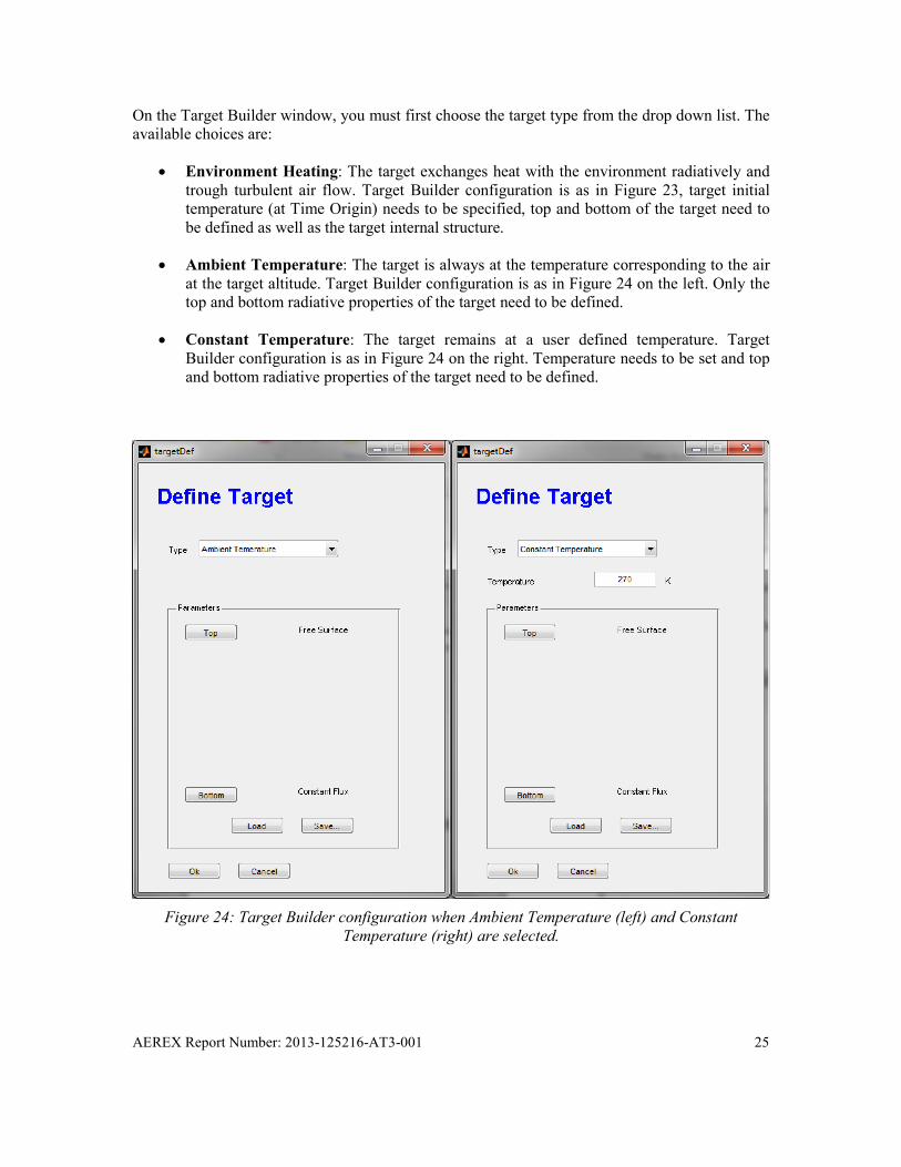
On the Target Builder window, you must first choose the target type from the drop down list. The available choices are:

• Environment Heating: The target exchanges heat with the environment radiatively and trough turbulent air flow. Target Builder configuration is as in Figure 23, target initial temperature (at Time Origin) needs to be specified, top and bottom of the target need to be defined as well as the target internal structure.

• Ambient Temperature: The target is always at the temperature corresponding to the air at the target altitude. Target Builder configuration is as in Figure 24 on the left. Only the top and bottom radiative properties of the target need to be defined.

• Constant Temperature: The target remains at a user defined temperature. Target Builder configuration is as in Figure 24 on the right. Temperature needs to be set and top and bottom radiative properties of the target need to be defined.

Figure 24: Target Builder configuration when Ambient Temperature (left) and Constant

Temperature (right) are selected.


8.3.1 Specifying the top and bottom properties

For all target types, you are required to specify at least the top surface, and the bottom surface for the Environmental Heating type (although you can configure the bottom surface for the other types, it has no impact on the result). To configure the top or bottom surface, use the “Top” or “Bottom” buttons in the Parameters group. Doing this opens up the Target Boundary Definition screen (Figure 25).

Figure 25: Target Boundary Definition screen

You can choose from three different types of interfaces for the target bottom boundary, these are:

• Free: The surface is free to interact with the environment radiatively and trough air turbulent heat exchange. The parameters group looks like Figure 25. See below for more details.

• Constant Temperature: The surface is held at a constant temperature. The parameters group switches to Figure 26 (left). You are required to enter the temperature in Kelvin. This represents the case where a constant heat source is in contact with the surface.


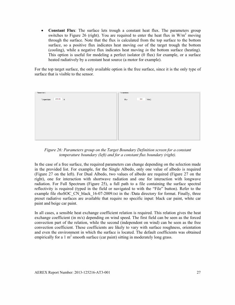
• Constant Flux: The surface lets trough a constant heat flux. The parameters group switches to Figure 26 (right). You are required to enter the heat flux in W/m2 moving through the surface. Note that the flux is calculated from the top surface to the bottom surface, so a positive flux indicates heat moving out of the target trough the bottom (cooling), while a negative flux indicates heat moving in the bottom surface (heating). This option is useful for modeling a perfect isolator (0 flux) for example, or a surface heated radiatively by a constant heat source (a motor for example).

For the top target surface, the only available option is the free surface, since it is the only type of surface that is visible to the sensor.

Figure 26: Parameters group on the Target Boundary Definition screen for a constant

temperature boundary (left) and for a constant flux boundary (right).

In the case of a free surface, the required parameters can change depending on the selection made in the provided list. For example, for the Single Albedo, only one value of albedo is required (Figure 27 on the left). For Dual Albedo, two values of albedo are required (Figure 27 on the right), one for interaction with shortwave radiation and one for interaction with longwave radiation. For Full Spectrum (Figure 25), a full path to a file containing the surface spectral reflectivity is required (typed in the field or navigated to with the “File” button). Refer to the example file rhoSOC_CN_black_16-07-2009.txt in the /Data directory for format. Finally, three preset radiative surfaces are available that require no specific input: black car paint, white car paint and beige car paint.

In all cases, a sensible heat exchange coefficient relation is required. This relation gives the heat exchange coefficient (in m/s) depending on wind speed. The first field can be seen as the forced convection part of the relation, while the second (independent on wind) can be seen as the free convection coefficient. These coefficients are likely to vary with surface roughness, orientation and even the environment in which the surface is located. The default coefficients was obtained empirically for a 1 m2 smooth surface (car paint) sitting in moderately long grass.


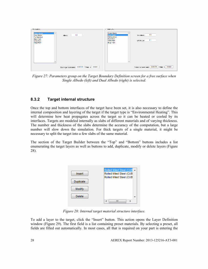
Figure 27: Parameters group on the Target Boundary Definition screen for a free surface when

Single Albedo (left) and Dual Albedo (right) is selected.

8.3.2 Target internal structure

Once the top and bottom interfaces of the target have been set, it is also necessary to define the internal composition and layering of the target if the target type is “Environmental Heating”. This will determine how heat propagates across the target so it can be heated or cooled by its interfaces. Targets are modeled internally as slabs of different materials and of varying thickness. The number and thickness of the slabs determine the accuracy of the computation, but a large number will slow down the simulation. For thick targets of a single material, it might be necessary to split the target into a few slabs of the same material.

The section of the Target Builder between the “Top” and “Bottom” buttons includes a list enumerating the target layers as well as buttons to add, duplicate, modify or delete layers (Figure 28).

Figure 28: Internal target material structure interface.

To add a layer to the target, click the “Insert” button. This action opens the Layer Definition window (Figure 29). The first field is a list containing preset materials. By selecting a preset, all fields are filled out automatically. In most cases, all that is required on your part is entering the


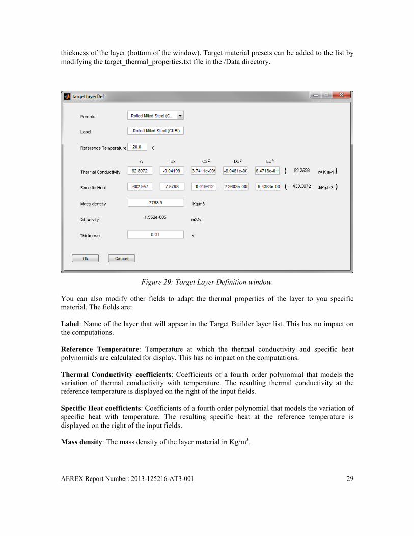
thickness of the layer (bottom of the window). Target material presets can be added to the list by modifying the target_thermal_properties.txt file in the /Data directory.

Figure 29: Target Layer Definition window.

You can also modify other fields to adapt the thermal properties of the layer to you specific material. The fields are:

Label: Name of the layer that will appear in the Target Builder layer list. This has no impact on the computations.

Reference Temperature: Temperature at which the thermal conductivity and specific heat polynomials are calculated for display. This has no impact on the computations.

Thermal Conductivity coefficients: Coefficients of a fourth order polynomial that models the variation of thermal conductivity with temperature. The resulting thermal conductivity at the reference temperature is displayed on the right of the input fields.

Specific Heat coefficients: Coefficients of a fourth order polynomial that models the variation of specific heat with temperature. The resulting specific heat at the reference temperature is displayed on the right of the input fields.

Mass density: The mass density of the layer material in Kg/m3.


Diffusivity (non-modifiable): The thermal diffusivity of the layer material, automatically calculated from the thermal conductivity, specific heat and mass density and non-modifiable.

Thickness: The thickness of the layer in meters.

Once the layer is defined, press the “Ok” button on the lower left corner of the window or press the “Cancel” button to discard modifications.

Often, a target will be made up of multiple identical layers for increased accuracy in solving the thermal propagation differential equation. You can duplicate an existing layer by selecting the layer and pressing the “Duplicate” button.

To modify an existing layer, use the “Modify” button. The Layer Definition window opens with the current material properties. Hereafter, the process is identical to adding a layer.

To delete an existing layer, select the layer to be deleted, and press the “Delete” button.

Once you are done with defining the target top, bottom and internal structure, you can save the target in a .tgt file by pressing the “Save…” button in the parameters group of the Target Definition window (Figure 23). This only saves the top, bottom and internal structure of the target, but not the target type or initial temperature. Later on, you can reload your target by clicking the “Load…” button.


9 Results panel

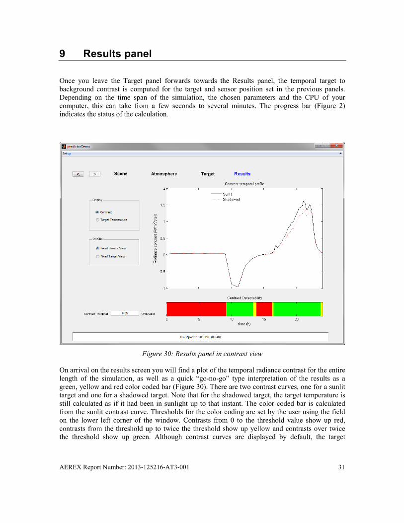
Once you leave the Target panel forwards towards the Results panel, the temporal target to background contrast is computed for the target and sensor position set in the previous panels. Depending on the time span of the simulation, the chosen parameters and the CPU of your computer, this can take from a few seconds to several minutes. The progress bar (Figure 2) indicates the status of the calculation.

Figure 30: Results panel in contrast view

On arrival on the results screen you will find a plot of the temporal radiance contrast for the entire length of the simulation, as well as a quick “go-no-go” type interpretation of the results as a green, yellow and red color coded bar (Figure 30). There are two contrast curves, one for a sunlit target and one for a shadowed target. Note that for the shadowed target, the target temperature is still calculated as if it had been in sunlight up to that instant. The color coded bar is calculated from the sunlit contrast curve. Thresholds for the color coding are set by the user using the field on the lower left corner of the window. Contrasts from 0 to the threshold value show up red, contrasts from the threshold up to twice the threshold show up yellow and contrasts over twice the threshold show up green. Although contrast curves are displayed by default, the target


temperature variations with time can also be viewed by selecting the “Target Temperature” option in the Display options group (Figure 31).

Figure 31: Results panel in target temperature view

If you hover your mouse pointer above the plotting area, a vertical line appears at the cursor position and the progress bar area displays the date, time and contrast. In the Ref. [4] example, the text string “09-Sept-2011 08:07:31 (-0.061)” appears. Once your mouse pointer is at the desired date and time, clicking on the plot area launches on of two spatial contrast calculations for that specific time depending on the option chosen in the On Click option group:

Fixed Sensor View: The sensor is fixed at the position and orientation set in the Scene panel. The target temperature is calculated at its position set in the Target panel. The target is then moved around in the sensor field of view, and the target to background contrast is plotted using the red-yellow-green color scheme according to the user set threshold (Figure 32). The results open in a new Matlab figure window.

Fixed Target View: The target is fixed at the position and orientation set in the Target panel. The sensor is then moved around the target in all areas where the sensor can see the target, and the target to background contrast is plotted using the red-yellow-green color scheme according to the user set threshold (Figure 33). The results open in a new Matlab figure window.


Figure 32: Fixed Sensor contrast map example.

Figure 33: Fixed target contrast map example


Note that some areas might not display the red-yellow-green color code either in the sensor field of view (in fixed sensor mode) or in the visible target area (if fixed target mode). An example of this can be seen in Figure 33 where the area below the target is white (the target is located at the point where all lines converge). This does not indicate a computation error. It most likely indicates that in these areas, the sensor is looking at the bottom of the target. Only the top of the target is actually “visible” from the sensor.


10 Additional information

For more information of the theoretical background behind the Contrast Predictor, please refer to the Contrast Predictor technical documentation [4].


References .....

[1] “Projet Optique Atmosphérique.” Proposal AAI-2012-125216, 2012. AEREX Avionique inc.

[2] © 2013 The MathWorks, Inc. MATLAB and Simulink are registered trademarks of The MathWorks, Inc. See www.mathworks.com/trademarks for a list of additional trademarks. Other product or brand names may be trademarks or registered trademarks of their respective holders.

[3] P.K. Acharya, A. Berk, G.P. Anderson, N.F. Larsen, S-Chee Tsay, and K.H. Stamnes, “MODTRAN4: Multiple Scattering and Bi-Directional Reflectance Distribution Function (BRDF) Upgrades to MODTRAN”, Proc. of SPIE, Optical Spectroscopy Techniques and Instrumentation for Atmospheric and Space Research, 3756, 19-21, July 1999.

[4] Ross, V and Gagné, G, “Simulation of sub pixel atmospherically degraded target detectability in cluttered scenes.”, AEREX Report No. 2013-125216-004, AEREX Avionics Inc., September 2013.


http://www.mathworks.com/trademarks

List of symbols/abbreviations/acronyms/initialisms

AMP Air mass parameter

CPU Computer Processing Unit

DRDC Defence Research & Development Canada

GUI Graphical User Interface

J Joule

m meter

NAM Navy aerosol model

K Kelvin

Kg Kilogram

sr steradian

W Watt

µm Micrometer
