Human Language Technologies: The 2015 Annual Conference of the North American Chapter of the ACL, pages 324–334,Denver, Colorado, May 31 – June 5, 2015. c©2015 Association for Computational Linguistics

Continuous Space Representations of Linguistic Typologyand their Application to Phylogenetic Inference

Yugo MurawakiGraduate School of Information Science and Electrical Engineering

Kyushu UniversityFukuoka, Japan

murawaki@ait.kyushu-u.ac.jp

Abstract

For phylogenetic inference, linguistic typol-ogy is a promising alternative to lexical evi-dence because it allows us to compare an ar-bitrary pair of languages. A challenging prob-lem with typology-based phylogenetic infer-ence is that the changes of typological fea-tures over time are less intuitive than thoseof lexical features. In this paper, we workon reconstructing typologically natural ances-tors To do this, we leverage dependenciesamong typological features. We first repre-sent each language by continuous latent com-ponents that capture feature dependencies. Wethen combine them with a typology evaluatorthat distinguishes typologically natural lan-guages from other possible combinations offeatures. We perform phylogenetic inferencein the continuous space and use the evalua-tor to ensure the typological naturalness of in-ferred ancestors. We show that the proposedmethod reconstructs known language fami-lies more accurately than baseline methods.Lastly, assuming the monogenesis hypothesis,we attempt to reconstruct a common ancestorof the world’s languages.

1 IntroductionLinguistic typology is a cross-linguistic study thatclassifies the world’s languages according to struc-tural properties such as complexity of syllable struc-ture and object-verb ordering. The availability of alarge typology database (Haspelmath et al., 2005)makes it possible to take computational approachesto this area of study (Daume III and Campbell, 2007;Georgi et al., 2010; Rama and Kolachina, 2012). In

this paper, we consider its application to phyloge-netic inference. We aim at reconstructing evolution-ary trees that illustrate how modern languages havedescended from common ancestors.

Typological features have two advantages overother linguistic traits. First, they allow us to com-pare an arbitrary pair of languages. By contrast,historical linguistics has worked on regular soundchanges (see (Bouchard-Cote et al., 2013) for com-putational models). Glottochronology and computa-tional phylogenetics make use of the presence andabsence of lexical items (Swadesh, 1952; Gray andAtkinson, 2003). All these approaches require thatcertain sets of cognates, or words with common et-ymological origins, are shared by the languages inquestion. For this reason, it is hardly possible to uselexical evidence to search for external relations in-volving language isolates and tiny language familiessuch as Ainu, Basque, and Japanese. For these lan-guages, typology can be seen as the last hope.

The second advantage is that typological featuresare potentially capable of tracing evolutionary his-tory on the order of 10,000 years because theychange far more slowly than lexical traits. A glot-tochronological study indicates that even if Japaneseis genetically related to Korean, they diverged froma common ancestor no earlier than 6,700 yearsago (Hattori, 1999). Even the basic vocabulary van-ishes so rapidly that after some 6,000 years, the re-tention rate becomes comparable to chance similar-ity. By contrast, the word order of Japanese, for ex-ample is astonishingly stable. It remains intact fromthe earliest attested data. Thus we argue that if wemanage to develop a statistical model of typological

324

Munda Mon-Khmergrammar synthetic analyticword order head-last, OV, postpositional head-first, VO, prepositionalaffixation pre/infixing, suffixing pre/infixing or isolatingfusion agglutinative fusionalconsonants stable/assimilative shifting/dissimilativevowels harmonizing/stable reducing/diphthongizing

Table 1: Typological comparison of the Munda and Mon-Khmer branches of the Austroasiatic languages.An abridged version of Table 1 of (Donegan and Stampe, 2004).

changes with predictive power, we can understand amuch deeper past.

A challenging problem with typology-based in-ference is that the changes of typological featuresover time are less intuitive than those of lexical fea-tures. Regular sound changes have been well knownsince the time of the Neogrammarians. The bi-nary representations of lexical items commonly usedin computational phylogenetics correspond to theirtheir presence and absence. The alternations of eachfeature value can be straightforwardly interpreted asthe birth and death (Le Quesne, 1974) of a lexicalitem. By contrast, it is difficult to understand how alanguage switches from SOV to SVO.

Practically speaking, since each language is rep-resented by a vector of categorical features, we caneasily perform distance-based hierarchical cluster-ing. Still, the extent to which the resultant treereflects evolutionary history is unclear. Teh et al.(2008) proposed a generative model for hierarchicalclustering, which straightforwardly explains evolu-tionary history. However, features used in their ex-periments were binarized in a one-versus-rest man-ner (i.e., expanding a feature with K possible val-ues into K binary features) (Daume III and Camp-bell, 2007) although the model itself had an abil-ity to handle categorical values. With the indepen-dence assumption of binary features, the model waslikely to reconstruct ancestors with logically impos-sible states.

Typological studies have shown that dependen-cies among typological features are not limited tothe categorical constraints. For example, object-verb ordering is said to imply adjective-noun order-ing (Greenberg, 1963). A natural question arises asto what would happen to adjective-noun ordering ifobject-verb ordering were altered. While dependen-cies among feature pairs were discussed in previous

studies (Greenberg, 1978; Dunn et al., 2011), depen-dencies among more than two features are yet to beexploited.

To gain a better insight into typological changes,we take Austroasiatic languages as an example. Ta-ble 1 compares some typological features of theMunda and Mon-Khmer branches. Although theirgenetic relationship was firmly established, they arealmost opposite in structure. Their common an-cestor is considered to have been Mon-Khmer-like.This indicates that the holistic changes have hap-pened in the Munda branch (Donegan and Stampe,2004). To generalize from this example, we suggestthe following hypotheses:

1. The holistic polarization can be explained bylatent components that control dependenciesamong observable features.

2. Typological changes can occur in a way suchthat typologically unnatural intermediate statesare avoided.

To incorporate these hypotheses, we propose con-tinuous space representations of linguistic typology.Specifically, we use an autoencoder (see (Bengio,2009) for a review) to map each language into thelatent space. In analogy with principal componentanalysis (PCA), each element of the encoded vec-tor is referred to as a component. We combine theautoencoder with a typology evaluator that distin-guishes typologically natural languages from otherpossible combinations of features.

Armed with the typology evaluator, we performphylogenetic inference in the continuous space. Theevaluator ensures that inferred ancestors are alsotypologically natural. The inference procedure isguided by known language families so that eachcomponent’s stability with respect to evolutionaryhistory can be learned. To evaluate the proposedmethod, we hide some trees to see how well theyare reconstructed.

325

Lastly, we build a binary tree on top of knownlanguage families. This experiment is based on acontroversial assumption that the world’s languagesdescend from one common ancestor. Our goal hereis not to address the validity of the monogenesis hy-pothesis. Rather, we address the questions of howthe common ancestor looked like if it existed andhow modern languages have evolved from it.

2 Related WorkIn linguistic typology, much attention has beengiven to non-tree-like evolution (Trubetzkoy, 1928).Daume III (2009) incorporated linguistic areas intoa phylogenetic model and reported that the extendedmodel outperformed a simple tree model. This re-sult motivates us to use known language families forsupervision rather than to perform phylogenetic in-ference in purely unsupervised settings.

Dunn et al. (2011) applied a state-process modelto reference phylogenetic trees to test if a pair offeatures is independent. The model they adoptedcan hardly be extended to handle multiple features.They separately applied the model to each lan-guage family and claimed that most dependencieswere lineage-specific rather than universal tenden-cies. However, each known language family is soshallow in time depth that few feature changes canbe observed in it (Croft et al., 2011). We mitigatedata sparsity by letting our model share parametersamong language families all over the world.

3 Data and Preprocessing3.1 Typology Database and Phylogenetic TreesThe typology database we used is the World Atlasof Language Structures (WALS) (Haspelmath et al.,2005). As of 2014, it contains 2,679 languages and192 typological features. It covers less than 15% ofthe possible language/feature pairs, however.

WALS provides phylogenetic trees but they onlyhave two layers above individual languages: fam-ily and genus. Language families include Indo-European, Austronesian and Niger-Congo, and gen-era within Indo-European include Germanic, In-dic and Slavic. For more detailed trees, weused hierarchical classifications provided by Ethno-logue (Lewis et al., 2014). The mapping betweenWALS and Ethnologue was done using ISO 639-3language codes. We manually corrected some obso-lete language codes used by WALS and dropped lan-

guages without language codes. We also excludedlanguages labeled by Ethnologue as Deaf sign lan-guage, Mixed language, Creole or Unclassified. Forboth WALS and Ethnologue trees, we removed in-termediate nodes that had only one child. Languageisolates were treated as family trees of their own.We obtained 193 family trees for WALS and 189 forEthnologue.

We made no further modifications to the trees al-though we were aware that some language familiesand their subgroups were highly controversial. Inthe future work, the Altaic language family, for ex-ample, should be disassembled into Turkic, Mon-golic and Tungusic to test if the Altaic hypothesisis valid (Vovin, 2005).

Next, we removed features with low coverage.Some features such as “Inclusive/Exclusive Formsin Pama-Nyungan” (39B) and “Irregular Negativesin Sign Languages” (139A) were not supposed tocover the world. We selected 98 features that cov-ered at least 10% of languages.1

We used the original, categorical feature values.The mergers of some fine-grained feature valuesseem desirable (Daume III and Campbell, 2007;Greenhill et al., 2010; Dunn et al., 2011). Some fea-tures like “Consonant Inventories” might be betterrepresented as real-valued features. We leave themfor future work.

In the end, we created two sets of data. The firstset PARTIAL was used to train the typology evalua-tor. We selected 887 languages that covered at least30% of features. The second set FULL was for phy-logenetic inference. We chose language families ineach of which at least 30% of features were coveredby one or more languages in the family. The num-bers of language families (including language iso-lates) were reduced to 103 for WALS and 110 forEthnologue.

3.2 Missing Data ImputationWe imputed missing data using the R package miss-MDA (Josse et al., 2012). It handled missing val-ues using multiple correspondence analysis (MCA).Specifically, we used the imputeMCA function to

1Additional cleanup is needed. For example, the high-coverage feature “The Position of Negative Morphemes in SOVLanguages” (144L) is not defined for non-SOV languages. Anatural solution is to add another feature value (Undefined).

326

0.21 0.84 0.03…

2 …2 0 33

0.01 0.00 0.99…0.92 0.02 0.000.01 0.01

0 0 1…1 0 00 0

0 0 1…1 0 00 0

2 …2 0 33

binarize the categorical vector

encode using the autoencoder

decode using the autoencoder

binarize according to categorical constraints

debinarize the binary vector

v

x

h

Figure 1: Representations of a language.

predict missing feature values. The substituted dataare used (1) to train the typology evaluator and (2)to initialize phylogenetic inference.

To evaluate the performance of missing data im-putation, we hid some known features to see howwell they were predicted. A 10-fold cross-validationtest using the PARTIAL dataset showed that 64.6% offeature values were predicted correctly. It consider-ably outperformed (1) the random baseline of 22.4%and (2) the most-frequent-value baseline of 28.1%.Thus our assumption of dependencies among fea-tures was confirmed.

4 Typology EvaluatorWe use a combination of an autoencoder to trans-form typological features into continuous latentcomponents, and an energy-based model to evaluatehow a given feature vector is typologically natural.

We begin with the autoencoder. Figure 1 showsvarious representations of a language. The origi-nal feature representation v is a vector of categoricalfeatures. v is binarized into x ∈ {0, 1}d0 in a one-versus-rest manner. x is mapped by an encoder to alatent representation h ∈ [0, 1]d1 , in which d1 is thedimension of the latent space:

h = s(Wex + be),

where s is the sigmoid function, and matrix We andvector be are weight parameters to be estimated. Adecoder then maps h back to x′ through a similartransformation:

x′ = s(Wdh + bd).

We use tied weights: Wd = WTe . Note that x′ is

a real vector. To recover a categorical vector, weneed to first binarize x′ according to categorical con-straints and then to debinarize the resultant vector.

The training objective of the autoencoder alone isto minimize cross-entropy of reconstruction:

LAE(x, x′) = −d∑

k=1

xk log x′k+(1−xk) log(1−x′

k),

where xk is the k-th element of x.Next, we plug an energy-based model into the au-

toencoder. It gives a probability to x.

p(x) =exp(WT

s g)∑x′ exp(WT

s g′),

g = s(Wlh + bl),

where vector Ws, matrix Wl and bias term bl arethe weights to be estimated. h is mapped to g ∈[0, 1]d2 before evaluation. This transformation ismotivated by our speculation that typologically nat-ural languages may not be linearly separable fromunnatural ones in the latent space since biplots ofprincipal components of PCA often show sinusoidalwaves (Novembre and Stephens, 2008). The denom-inator sums over all possible states of x′, includingthose which violate categorical constraints. By max-imizing the average log probability of training data,we can distinguish typologically natural languagesfrom other possible combinations of features.

Given a set of N languages with missing data im-puted,2 our training objective is to maximize the fol-lowing:

N∑i=1

(−LAE(xi, x′i) + C log p(xi))),

where C is some constant. Weights are optimizedby the gradient-based AdaGrad algorithm (Duchi etal., 2011) with a mini-batch. A problem with thisoptimization is that the derivative of the second termcontains an expectation that involves a summationover all possible states of x′, which is computa-tionally intractable. Inspired by contrastive diver-gence (Hinton, 2002), we do not compute the ex-pectation exactly but approximate it by few negativesamples collected from Gibbs samplers.

4.1 Mixing Languages: An ExperimentTo analyze the continuous space representations, wegenerated mixtures of two languages, which were

2We tried a joint inference of weight optimization and miss-ing data imputation but dropped it for its instability. A cross-validation test revealed that the joint inference caused a big ac-curacy drop in missing data imputation.

327

-60

-40

-20

0

20

40

60

80

100

0 0.2 0.4 0.6 0.8 1

log

pro

b +

C

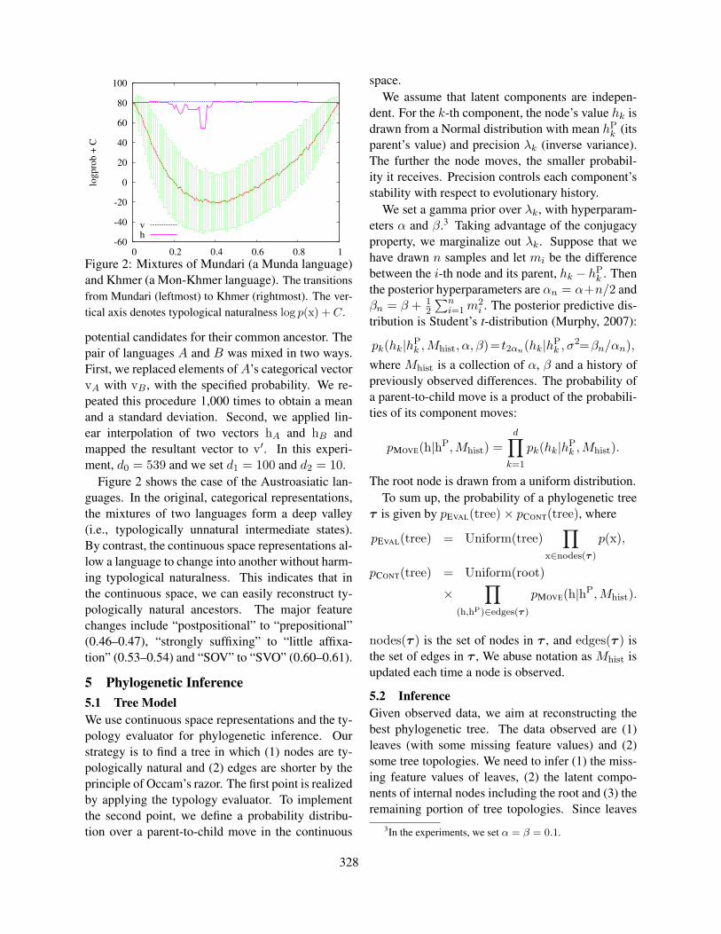
vh

Figure 2: Mixtures of Mundari (a Munda language)and Khmer (a Mon-Khmer language). The transitionsfrom Mundari (leftmost) to Khmer (rightmost). The ver-tical axis denotes typological naturalness log p(x) + C.

potential candidates for their common ancestor. Thepair of languages A and B was mixed in two ways.First, we replaced elements of A’s categorical vectorvA with vB , with the specified probability. We re-peated this procedure 1,000 times to obtain a meanand a standard deviation. Second, we applied lin-ear interpolation of two vectors hA and hB andmapped the resultant vector to v′. In this experi-ment, d0 = 539 and we set d1 = 100 and d2 = 10.

Figure 2 shows the case of the Austroasiatic lan-guages. In the original, categorical representations,the mixtures of two languages form a deep valley(i.e., typologically unnatural intermediate states).By contrast, the continuous space representations al-low a language to change into another without harm-ing typological naturalness. This indicates that inthe continuous space, we can easily reconstruct ty-pologically natural ancestors. The major featurechanges include “postpositional” to “prepositional”(0.46–0.47), “strongly suffixing” to “little affixa-tion” (0.53–0.54) and “SOV” to “SVO” (0.60–0.61).

5 Phylogenetic Inference5.1 Tree ModelWe use continuous space representations and the ty-pology evaluator for phylogenetic inference. Ourstrategy is to find a tree in which (1) nodes are ty-pologically natural and (2) edges are shorter by theprinciple of Occam’s razor. The first point is realizedby applying the typology evaluator. To implementthe second point, we define a probability distribu-tion over a parent-to-child move in the continuous

space.We assume that latent components are indepen-

dent. For the k-th component, the node’s value hk isdrawn from a Normal distribution with mean hP

k (itsparent’s value) and precision λk (inverse variance).The further the node moves, the smaller probabil-ity it receives. Precision controls each component’sstability with respect to evolutionary history.

We set a gamma prior over λk, with hyperparam-eters α and β.3 Taking advantage of the conjugacyproperty, we marginalize out λk. Suppose that wehave drawn n samples and let mi be the differencebetween the i-th node and its parent, hk − hP

k . Thenthe posterior hyperparameters are αn = α+n/2 andβn = β + 1

2

∑ni=1 m2

i . The posterior predictive dis-tribution is Student’s t-distribution (Murphy, 2007):

pk(hk|hPk ,Mhist, α, β)= t2αn(hk|hP

k , σ2=βn/αn),where Mhist is a collection of α, β and a history ofpreviously observed differences. The probability ofa parent-to-child move is a product of the probabili-ties of its component moves:

pMOVE(h|hP,Mhist) =d∏

k=1

pk(hk|hPk , Mhist).

The root node is drawn from a uniform distribution.To sum up, the probability of a phylogenetic tree

τ is given by pEVAL(tree)× pCONT(tree), where

pEVAL(tree) = Uniform(tree)∏

x∈nodes(τ )

p(x),

pCONT(tree) = Uniform(root)

×∏

(h,hP)∈edges(τ )

pMOVE(h|hP,Mhist).

nodes(τ ) is the set of nodes in τ , and edges(τ ) isthe set of edges in τ , We abuse notation as Mhist isupdated each time a node is observed.

5.2 InferenceGiven observed data, we aim at reconstructing thebest phylogenetic tree. The data observed are (1)leaves (with some missing feature values) and (2)some tree topologies. We need to infer (1) the miss-ing feature values of leaves, (2) the latent compo-nents of internal nodes including the root and (3) theremaining portion of tree topologies. Since leaves

3In the experiments, we set α = β = 0.1.

328

P

C1

S

C2

(a)

P

C1

S

C2

(b)

P

C1

S

C2

(c)

P

C2

S

C1

(d)

P

C1

S

C2

(e)

Figure 3: SWAP operator. The gray circle is the target node. Its parent P, sibling S and two children C1 andC2 are shown. (a) The current state. (b–e) The proposed states. (b–c) The topology remains the same butthe target is moved toward C1 and C2, respectively. (d) C1 is swapped for S. (e) C2 is swapped for S.

are tied to observed categorical vectors, our infer-ence procedures also work on them. We map cate-gorical vectors into the latent space every time weattempt to change a feature value. By contrast, weadopt latent vectors as the primary representationsof internal nodes.

Take the Indo-European language family for ex-ample. Its tree topology is given but the states ofits internal nodes such as Indo-European, Germanicand Indic need to be inferred. Dutch has some miss-ing feature values. Although they have been imputedwith multiple correspondence analysis, its close rel-atives such as Danish and German might be helpfulfor better estimation.

We need to infer portions of tree topologies eventhough a set of trees (language families) is given. Toevaluate the performance of phylogenetic inference,we hide some trees to see how well they are recon-structed. To reconstruct a common ancestor of theworld’s languages, we build a binary tree on top ofthe set of trees. Note that while we only infer binarytrees, a node may have more than two children in thefixed portions of tree topologies.

We use Gibbs sampling for inference. We definefour operators, CAT, COMP, SWAP and MOVE. Thefirst tree operators correspond to missing feature val-ues, latent components and tree topologies, respec-tively.

CAT – For the target categorical feature of a leafnode, we sample from K possible values. Let x′ be abinary feature representation with the target featurevalue altered, let hP be the state of the node’s parent,and let h′ = s(Wex′+be). The probability of choos-ing x′ is proportional to p(x′) pMOVE(h′|hP,Mhist),where h is removed from the history. The second

term is omitted if the target node has no parent.4

COMP – For the target k-th component of aninternal node, we choose its new value using theMetropolis algorithm. It stochastically proposesa new state and accepts it with some probabil-ity. If the proposal is rejected, the current stateis reused as the next state. The proposal distribu-tion Q(h′

k|hk) is a Gaussian distribution centeredat hk. The acceptance probability is a(hk, h

′k) =

min(1, P (h′k)/P (hk)), where P (h′

k) is defined as

P (h′k) = p(x′) pMOVE(h′|hP,Mhist)∏

hC∈children(h′)

pMOVE(hC|h′, Mhist)

where children(h′) is the set of the target node’schildren.

SWAP – For the target internal node (which cannotbe the root), we use the Metropolis-Hastings algo-rithm to locally rearrange its neighborhood in a waysimilar to Li et al. (2000). We first propose a newstate as illustrated in Figure 3. The target node hasa parent P, a sibling S and two children C1 and C2.From among S, C1 and C2, we choose two nodes.If C1 and C2 are chosen, the topology remains thesame; otherwise S is swapped for one of the node’schildren. It is shown that one topology can be trans-formed into any other topology in a finite number ofsteps (Li et al., 2000).

To improve mobility, we also move the targetnode toward C1, C2 or S, depending on the pro-posed topology. Here the selected node is denotedby ∗. We first draw r′ from a log-normal distri-bution whose underlying Gaussian distribution has

4It is easy to extend the operator to handle internal nodessupplied with some categorical features.

329

mean −1 and variance 1. The target’s proposed stateis h′ = (1 − r′)h + r′h∗. r′ can be greater than 1,and in that case, the proposed state h′ is more distantfrom h∗ than the current state h. This ensures thatthe transition is reversible because r = 1/r′. Theacceptance probability can be calculated in a similarmanner to that described for COMP.

MOVE – Propose to move the target internal node,without swapping its neighbors.

For initialization, missing feature values are im-puted by missMDA. The initial tree is constructed bydistance-based agglomerative clustering. The stateof an internal node is set to the average of those ofits children.

6 Experiments6.1 Reconstruction of Known Family Trees6.1.1 Data and Method

We first conducted a quantitative evaluation ofphylogenetic inference, using known family trees.We ran 5-fold cross-validations. For each of WALSand Ethnologue, we subdivided a set of languagefamilies into 5 subsets with roughly the same num-ber of leaves. Because of some huge language fami-lies, the number of language families per subset wasuneven. We disassembled family trees in the targetsubset and to let the model reconstruct a binary treefor each language family. Unlike ordinary held-outevaluation, this experiment used all data for infer-ence at once.

6.1.2 Model SettingsWe used the parameter settings described in Sec-

tion 4.1. For phylogenetic inference, we ran 9,000burn-in iterations after which we collected 100 sam-ples at an interval of 10 iterations.

For comparison, we performed average-link ag-glomerative clustering (ALC). It has two variants,ALC-CAT and ALC-CONT. ALC-CAT worked oncategorical features and used the ratio of disagree-ment as a distance metric. ALC-CONT performedclustering in the continuous space, using cosine dis-tance. In other words, we can examine the effectsof the typology evaluator and precision parameters.For these models, missing feature values are im-puted by missMDA.

6.1.3 Evaluation MeasuresWe present purity (Heller and Ghahramani, 2005),

subtree (Teh et al., 2008) and outlier fraction

(a)

(b)

(c)

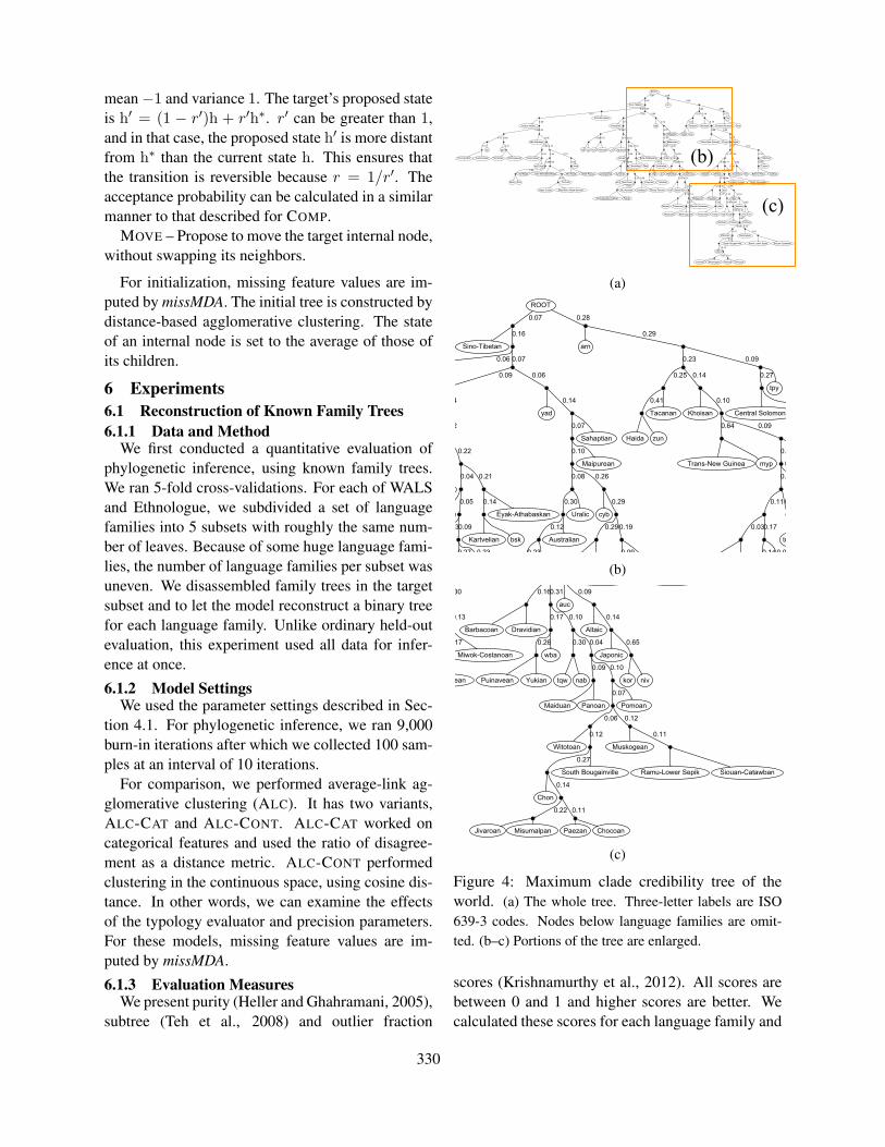
Figure 4: Maximum clade credibility tree of theworld. (a) The whole tree. Three-letter labels are ISO639-3 codes. Nodes below language families are omit-ted. (b–c) Portions of the tree are enlarged.

scores (Krishnamurthy et al., 2012). All scores arebetween 0 and 1 and higher scores are better. Wecalculated these scores for each language family and

330

WALS Ethnologuepurity subtree outlier outlier

ALC-CAT .500 .557 .608 .626 .343 .330 .358 .398ALC-CONT .503 .557 .630 .630 .343 .330 .353 .395Proposed .522 .572 .603 .651 .351 .346 .356 .394

Table 2: Results of the reconstruction of known family trees. Macro-averages are followed by micro-averages.

report macro- and micro-averages. Only non-trivialfamily trees (trees with more than two children)were considered.

Purity and subtree scores compare inferred treeswith gold-standard class labels. In WALS, generawere treated as class labels because they were theonly intermediate layer between families and leaves.By contrast, Ethnologue provided more complextrees and we were unable to assign one class labelto each language. For this reason, only outlier frac-tion scores are reported for Ethnologue.

6.1.4 ResultsTable 2 shows the scores for reconstructed fam-

ily trees. The proposed method outperformed thebaselines in 5 out of 8 metrics. Three methods per-formed almost equally for Ethnologue. We suspectthat typological features reflect long term trends incomparison to Ethnologue’s fine-grained classifica-tion. For WALS, the proposed method was beatenby average-link agglomerative clustering only inthe macro-average of subtree scores. One pos-sible explanation is randomness of the proposedmethod. Apparently, random sampling distributederrors more evenly than deterministic clustering. Itwas penalized more often by subtree scores becausethey required that all leaves of an internal node be-longed to the same class.

6.2 Reconstruction of a Common Ancestor ofthe World’s Languages

We reconstructed a single tree that covers the world.To do this, we build a binary tree on top of knownlanguage families, a product of historical linguistics.It is generally said that historical linguistics cannotgo far beyond 6,000–7,000 years (Nichols, 2011).Here we attempt to break the brick wall.

It is no surprise that this experiment is full ofproblems and difficulties. No quantitative evalua-tion is possible. Underlying assumptions are ques-tionable. No one knows for sure if there was sucha thing as one common ancestor of all modern lan-

0

5

10

15

20

25

0 0.02 0.04 0.06 0.08 0.1

freq

uen

cy

variance

Figure 5: Histogram of posterior variances σ2 =βn/αn of the 4,000th sample.

0

0.2

0.4

0.6

0.8

1

0 0.2 0.4 0.6 0.8 1

2n

d s

mal

lest

co

mp

on

ent

smallest component

leavesinternal

root

Figure 6: Scatter plot of languages using thecomponents with the two smallest variances.

guages. Moreover, language capacity of humans, inaddition to languages themselves, is likely to haveevolved over time (Nichols, 2011). This casts doubton the applicability of the typology evaluator, whichis trained on modern languages, to languages of fardistant past. Nevertheless, it is fascinating to makeinference on the world’s ancestral languages.

We used Ethnologue as the known tree topologies.For Gibbs sampling, we ran 3,000 burn-in iterationsafter which we collected 100 samples at an intervalof 10 iterations.

Figure 4 shows a reconstructed tree. To summa-rize multiple sample trees, we constructed a max-imum clade credibility tree. For each clade (a setof all leaves that share a common ancestor), we cal-culated the fraction of times it appears in the col-lected samples, which we call a support in this pa-

331

Features Frequencies/Values

Consonant Inventories95 Average5 Moderately small

Vowel Quality Inventories85 Average (5-6)15 Small (2-4)

Syllable Structure100 Moderately complex

0 Complex

Coding of Nominal Plurality

97 Plural suffix2 Plural word1 No plural0 Plural clitic

Order of Numeral and Noun61 Noun-Numeral39 Numeral-Noun

Position of Case Affixes61 No case affixes or adp. clitics39 Case suffixes

Ord. of SOV61 SOV38 SVO1 No dominant order

Ord. of Adposition and NP91 Postpositions9 Prepositions

Ord. of Adjective and Noun87 Noun-Adjective13 Adjective-Noun

Table 3: Some features of the world’s ancestor withsample frequencies.

per. A tree was scored by the product of supports ofall clades within it, and we created a tree that maxi-mized the score. Each edge label shows the supportof the corresponding clade. As indicated by gen-erally low supports, the sample trees were very un-stable. Some geographically distant groups of lan-guages were clustered near the bottom. We partiallyattribute this to the underspecificity of linguistic ty-pology: even if a pair of languages shares the samefeature vector, they are not necessarily the same lan-guage. This problem might be eased by incorporat-ing geospatial information into phylogenetic infer-ence (Bouckaert et al., 2012).

Table 3 shows some features of the root. The re-constructed ancestor is moderate in phonological ty-pology, uses suffixing in morphology and prefers theSOV word order. The inferred word order agreeswith speculations given by previous studies (Mau-rits and Griffiths, 2014).

Figure 5 shows the histogram of variance parame-ters. Some latent components had smaller variancesand thus were more stable with respect to evolution-ary history. Figure 6 displays languages using thecomponents with the two smallest variances. UnlikePCA plots, data concentrated at the edges.

We used a geometric mean of pMOVE of multi-ple samples to calculate how a modern language is

Rank Language Classificatoin Logprob.1(Japanese)Japonic 76.82Shuri Japonic -37.73Khalkha Altaic>Mongolic -200.04Lepcha Sino-Tibetan>Tibeto-Burman -201.95Chuvash Altaic>Turkic -205.56Deuri Sino-Tibetan>Tibeto-Burman -218.37Urum Altaic>Turkic -218.68Ordos Altaic>Mongolic -219.09Uzbek Altaic>Turkic -219.6

10Archi N. Caucasian>E. Caucasian -221.5131Korean (isolate) -265.7493Ainu (isolate) -409.9

Table 4: Modern languages ranked by the similarityto Japanese.

similar to another. The case of Japanese is shownin Table 4. This ranked list is considerably dif-ferent from that of disagreement rates of categor-ical vectors (Spearman’s ρ = 0.76). When fea-tures’ stability with respect to evolutionary historyis considered, Japanese is less closer to Korean andAinu than to some Tibeto-Burman languages southof the Himalayas. As the importance of these mi-nor languages of Northeast India is recognized, theSino-Tibetan tree might be drastically revised in thefuture (Blench and Post, 2013). The least similarlanguages include the Malayo-Polynesian and Nilo-Saharan languages.

7 ConclusionIn this paper, we proposed continuous space repre-sentations of linguistic typology and used them forphylogenetic inference. Feature dependencies area major focus of linguistic typology, and typologydata have occasionally been used for computationalphylogenetics. To our knowledge, however, we arethe first to integrate the two lines of research. Inaddition, the continuous space representations un-derlying interdependent discrete features are appli-cable to other data including phonological invento-ries (Moran et al., 2014).

We believe that typology provides important cluesfor long-term language change. The currently avail-able database only contains modern languages, butwe expect that data of some ancestral languagescould greatly facilitate computational approaches todiachronic linguistics.

AcknowledgmentThis work was partly supported by JSPS KAKENHIGrant Number 26730122.

332

References

Yoshua Bengio. 2009. Learning deep architectures forAI. Foundations and Trends in Machine Learning,2(1):1–127.

Roger Blench and Mark W. Post. 2013. Rethinking Sino-Tibetan phylogeny from the perspective of North EastIndian languages. In Nathan Hill and Tom Owen-Smith, editors, Trans-Himalayan Linguistics, pages71–104. De Gruyter.

Alexandre Bouchard-Cote, David Hall, Thomas L. Grif-fiths, and Dan Klein. 2013. Automated reconstruc-tion of ancient languages using probabilistic modelsof sound change. PNAS, 110(11):4224–4229.

Remco Bouckaert, Philippe Lemey, Michael Dunn, Si-mon J. Greenhill, Alexander V. Alekseyenko, Alexei J.Drummond, Russell D. Gray, Marc A. Suchard, andQuentin D. Atkinson. 2012. Mapping the origins andexpansion of the Indo-European language family. Sci-ence, 337(6097):957–960.

William Croft, Tanmoy Bhattacharya, Dave Klein-schmidt, D. Eric Smith, and T. Florian Jaeger. 2011.Greenbergian universals, diachrony, and statisticalanalyses. Linguistic Typology, 15(2):433–453.

Hal Daume III and Lyle Campbell. 2007. A Bayesianmodel for discovering typological implications. InACL, pages 65–72.

Hal Daume III. 2009. Non-parametric Bayesian areallinguistics. In HLT-NAACL, pages 593–601.

Patricia Donegan and David Stampe. 2004. Rhythm andthe synthetic drift of Munda. In Rajendra Singh, edi-tor, The Yearbook of South Asian Languages and Lin-guistics, pages 3–36. Mouton de Gruyter.

John Duchi, Elad Hazan, and Yoram Singer. 2011.Adaptive subgradient methods for online learning andstochastic optimization. The Journal of MachineLearning Research, 12:2121–2159.

Michael Dunn, Simon J. Greenhill, Stephen C. Levinson,and Russell D. Gray. 2011. Evolved structure of lan-guage shows lineage-specific trends in word-order uni-versals. Nature, 473(7345):79–82.

Ryan Georgi, Fei Xia, and William Lewis. 2010.Comparing language similarity across genetic andtypologically-based groupings. In COLING, pages385–393.

Russell D. Gray and Quentin D. Atkinson. 2003.Language-tree divergence times support the Ana-tolian theory of Indo-European origin. Nature,426(6965):435–439.

Joseph H. Greenberg, editor. 1963. Universals of lan-guage. MIT Press.

Joseph H. Greenberg. 1978. Diachrony, synchronyand language universals. In Joseph H. Greenberg,

Charles A. Ferguson, and Edith A. Moravesik, edi-tors, Universals of human language, volume 1. Stan-ford University Press.

Simon J. Greenhill, Quentin D. Atkinson, AndrewMeade, and Russel D. Gray. 2010. The shape andtempo of language evolution. Proc. of the Royal Soci-ety B, 277(1693):2443–2450.

Martin Haspelmath, Matthew Dryer, David Gil, andBernard Comrie, editors. 2005. The World Atlas ofLanguage Structures. Oxford University Press.

Shiro Hattori. 1999. Nihongo no keito (The Genealogyof Japanese). Iwanami Shoten.

Katherine A. Heller and Zoubin Ghahramani. 2005.Bayesian hierarchical clustering. In ICML, pages 297–304.

Geoffrey E. Hinton. 2002. Training products of expertsby minimizing contrastive divergence. Neural Com-putation, 14(8):1771–1800.

Julie Josse, Marie Chavent, Benot Liquet, and FrancoisHusson. 2012. Handling missing values with regular-ized iterative multiple correspondence analysis. Jour-nal of Classification, 29(1):91–116.

Akshay Krishnamurthy, Sivaraman Balakrishnan, MinXu, and Aarti Singh. 2012. Efficient active algorithmsfor hierarchical clustering. In ICML, pages 887–894.

Walter J. Le Quesne. 1974. The uniquely evolved char-acter concept and its cladistic application. SystematicBiology, 23(4):513–517.

M. Paul Lewis, Gary F. Simons, and Charles D. Fen-nig, editors. 2014. Ethnologue: Languages of theWorld, 17th Edition. SIL International. Online ver-sion: http://www.ethnologue.com.

Shuying Li, Dennis K. Pearl, and Hani Doss. 2000. Phy-logenetic tree construction using Markov chain MonteCarlo. Journal of the American Statistical Associa-tion, 95(450):493–508.

Luke Maurits and Thomas L. Griffiths. 2014. Tracing theroots of syntax with Bayesian phylogenetics. PNAS,111(37):13576–13581.

Steven Moran, Daniel McCloy, and Richard Wright, ed-itors. 2014. PHOIBLE Online. Max Planck Institutefor Evolutionary Anthropology, Leipzig.

Kevin P. Murphy. 2007. Conjugate Bayesian analysis ofthe Gaussian distribution. Technical report, Universityof British Columbia.

Johanna Nichols. 2011. Monogenesis or polygenesis: Asingle ancestral language for all humanity? In Mag-gie Tallerman and Kathleen R. Gibson, editors, TheOxford Handbook of Language Evolution, pages 558–572. Oxford Univ Press.

John Novembre and Matthew Stephens. 2008. Interpret-ing principal component analyses of spatial populationgenetic variation. Nature Genetics, 40(5):646–649.

333

Taraka Rama and Prasanth Kolachina. 2012. How goodare typological distances for determining genealogicalrelationships among languages? In COLING Posters,pages 975–984.

Morris Swadesh. 1952. Lexicostatistic dating of prehis-toric ethnic contacts. Proc. of American PhilosophicalSociety, 96:452–463.

Yee Whye Teh, Hal Daume III, and Daniel Roy. 2008.Bayesian agglomerative clustering with coalescents.In NIPS, pages 1473–1480.

Nikolai Sergeevich Trubetzkoy. 1928. Proposition 16. InActs of the First International Congress of Linguists,pages 17–18.

Alexander Vovin. 2005. The end of the Altaic contro-versy. Central Asiatic Journal, 49(1):71–132.

334