continuous decline in lower stratospheric ozone sets · pdf filecontinuous decline in lower...

Continuous decline in lower stratospheric ozoneoffsets ozone layer recoveryWilliam T. Ball1,2, Justin Alsing3, Daniel J. Mortlock4,5,6, Johannes Staehelin2,Joanna D. Haigh4,7, Thomas Peter2, Fiona Tummon2, Rene Stübi8,Andrea Stenke2, John Anderson9, Adam Bourassa10, Sean M. Davis11,12,Doug Degenstein10, Stacey Frith13,14, Lucien Froidevaux15, Chris Roth10,Viktoria Sofieva16, Ray Wang17, Jeannette Wild18,19, Pengfei Yu11,12,Jerald R. Ziemke14,20, and Eugene V. Rozanov1,2

1Physikalisch-Meteorologisches Observatorium Davos World Radiation Centre, Dorfstrasse 33,7260 Davos Dorf, Switzerland2Institute for Atmospheric and Climate Science, Swiss Federal Institute of Technology Zurich,Universitaetstrasse 16, CHN, CH-8092 Zurich, Switzerland3Center for Computational Astrophysics, Flatiron Institute, 162 5th Ave, New York, NY 10010,USA4Physics Department, Blackett Laboratory, Imperial College London, SW7 2AZ, UK5Department of Mathematics, Imperial College London, SW7 2AZ, UK6Department of Astronomy, Stockholms universitet, SE-106 91 Stockholm, Sweden7Grantham Institute - Climate Change and the Environment, Imperial College London, SW7 2AZ,UK8Federal Office of Meteorology and Climatology, MeteoSwiss, CH-1530 Payerne, Switzerland9Hampton University, Hampton, VA, USA10Institute of Space and Atmospheric Studies, University of Saskatchewan, Saskatoon, Canada11Cooperative Institute for Research in Environmental Sciences, University of Colorado, Boulder,CO, USA12NOAA Earth System Research Laboratory, Boulder, CO, USA13NASA Goddard Space Flight Center, Silver Spring, MD, USA14Science Systems and Applications Inc., Lanham, MD, USA15Jet Propulsion Laboratory, California Institute of Technology, Pasadena, CA, USA16Finnish Meteorological Institute, Helsinki, Finland17School of Earth and Atmospheric Sciences, Georgia Institute of Technology, Atlanta, GA, USA18NOAA/NWS/NCEP/Climate Prediction Center, College Park, MD, USA19Innovim LLC, Greenbelt, MD, USA20NASA Goddard Space Flight Center, Greenbelt, MD, USA

Correspondence to: W. T. Ball ([email protected])

1

Atmos. Chem. Phys. Discuss., https://doi.org/10.5194/acp-2017-862Manuscript under review for journal Atmos. Chem. Phys.Discussion started: 10 October 2017c© Author(s) 2017. CC BY 4.0 License.

Abstract. Ozone forms in the Earth’s atmosphere from the photodissociation of molecular oxy-

gen, primarily in the tropical stratosphere. It is then transported to the extratropics by the Brewer-

Dobson circulation (BDC), forming a protective ‘ozone layer’ around the globe. Human emissions of

halogen-containing ozone-depleting substances (hODSs) led to a decline in stratospheric ozone until

they were banned by the Montreal Protocol (MP), and since 1998 ozone in the upper stratosphere5

shows a likely recovery. Total column ozone (TCO) measurements of ozone between the Earth’s

surface and the top of the atmosphere, indicate that the ozone layer has stopped declining across

the globe, but no clear increase has been observed at latitudes outside the polar regions (60◦–90◦).

Here we report evidence from multiple satellite measurements that ozone in the lower stratosphere

between 60◦S and 60◦N has declined continuously since 1985. We find that, even though upper10

stratospheric ozone is recovering in response to the MP, the lower stratospheric changes more than

compensate for this, resulting in the conclusion that, globally (60◦S–60◦N), stratospheric column

ozone (StCO) continues to deplete. We find that globally, TCO appears to not have decreased be-

cause tropospheric column ozone (TrCO) increases, likely the result of human activity and harmful

to respiratory health, are compensating for the stratospheric decreases. The reason for the continued15

reduction of lower stratospheric ozone is not clear, models do not reproduce these trends, and so

the causes now urgently need to be established. Reductions in lower stratospheric ozone trends may

partly lead to a small reduction in the warming of the climate, but a reduced ozone layer may also

permit an increase in harmful ultra-violet (UV) radiation at the surface and would impact human and

ecosystem health.20

1 Introduction

The stratospheric ozone layer protects surface life from harmful solar ultraviolet radiation. In the

second half of the 20th century, halogen-containing ozone depleting substances (hODSs) resulting

from human activity, mainly in the form of chloroflurocarbons (CFCs), led to the decline of the

ozone layer (Molina and Rowland, 1974). The clearest example of ozone depletion was signified by25

the formation of an ozone hole over the Southern polar region, but even outside there was a clear

reduction in total coulmn ozone (TCO) (Farman et al., 1985; WMO/NASA, 1988; WMO, 2011,

2014). The Montreal Protocol came into effect in 1989, banning multiple substances responsible for

ozone layer depletion, and by 1997 it became apparent that a decline in TCO had ceased at almost

all non-polar latitudes.30

The general expectation is that global mean stratospheric column ozone (StCO) will increase as

hODSs continue to decline, but an attribution of increasing TCO to decreasing ODSs has not yet

been possible (WMO, 2014); a cooling stratosphere is also thought to aid the recovery of ozone

by slowing temperature-dependent reaction rates. Models predict that mean TCO will increase, but

2


this also remains uncertain since projections rely substantially on the CO2, N2O and CH4 emissions35

scenarios.

Only recently has a TCO recovery been detected during the austral spring (Solomon et al., 2016).

However, elsewhere observations of global TCO levels have remained stable since 2000 (WMO,

2014), with most latitudes displaying a positive, but non-significant, decadal trend (WMO, 2014).

Results from Frith et al. (2014) suggest a potential peak in positive trends around 2011, after which40

positive trends declined while uncertainties increased, despite longer timeseries.

In the past the attribution and identification of ozone recovery was made through multiple linear

regression (MLR) analysis with most studies considering either piecewise linear trends (PWLT)

to represent trends, with an inflection date usually at the end of 1997, or the equivalent effective

stratospheric chlorine (EESC) proxy to represent the influence of hODSs on ozone, which is a non-45

linear smoothly-varying proxy with an inflection date also around 1997 (Newman et al., 2007).

Two recent studies, Chehade et al. (2014) and Frith et al. (2014), both investigated changes in TCO

observations up to 2012 and 2013, respectively, and came to similar conclusions: trends using PWLT

or EESC prior to 1997 agree that ozone declined to a minimum in 1997, but from 1997 the use of the

EESC proxy suggests a significant and positive increase at all latitudes (larger at higher latitudes),50

while use of PWLT shows peaks at mid-latitudes but is generally lower and non-significant at most

latitudes outside the polar regions. These results suggest that attribution to EESC prior to 1997 is

the dominant contributor to the long-term trend, but after 1997 it may be less representative, or that

large dynamical variability is interfering with post-1997 trends. As both Chehade et al. (2014) and

Frith et al. (2014) note, the post-1997 EESC estimate is partially locked by the large decline during55

the pre-1998 period, while in PWLT the period to fix the estimate is not influenced by the latter or

earlier period, respectively. The consequence may be, then, that a significant post-1997 change in

TCO might indeed represent a hODS-related increase in ozone, but this may be embedded within

ozone that is not actually increasing, or increasing at a slower rate, as shown by the PWLT that

represents the overall timeseries without any specific physical attribution.60

Despite a lack of clear recovery in TCO, ozone in the upper stratosphere above 10 hPa appears to

be recovering, which has been reported with significant positive decadal trends in vertical profiles,

and altitude-latitude spatial maps, from multiple ozone composites that merge observations from

various space missions, especially at mid-latitudes (Kyrölä et al., 2013; Laine et al., 2014; WMO,

2014; Tummon et al., 2015; Harris et al., 2015; Steinbrecht et al., 2017; Ball et al., 2017; Sofieva65

et al., 2017; Bourassa et al., 2017). Trends in these results are almost always presented as percentage-

change per decade, which does not illuminate the contribution to the column ozone changes. Thus,

noting that total column may be increasing, and that upper stratospheric ozone is recovering, does not

mean that stratospheric ozone as a whole is increasing as counteracting trends in different layers of

the stratosphere, and troposphere, may counteract a TCO recovery. Indeed, if TCO does not display70

any significant changes since 1997, while the upper stratosphere displays significant increases, then

3


either the uncertainties due to unattributed dynamical variability interfere in the significance of the

trend determined through MLR, or there are counteracting trends at lower levels of the stratosphere,

or in the troposphere.

Suggestions of a decrease in lower stratospheric ozone have been presented elsewhere (Kyrölä75

et al., 2013; Gebhardt et al., 2014; Sioris et al., 2014; Nair et al., 2015; Vigouroux et al., 2015).

However, it has been difficult to confirm (WMO, 2014) because: (i) ozone is typically integrated

over wide latitude bands and/or total column ozone (TCO) is considered, both of which may lead

to cancellation of opposing trends; (ii) large dynamical variability unaccounted for in regression

analysis together with shorter timeseries lead to higher uncertainties (Tegtmeier et al., 2013); (iii)80

below 20 km there are large ozone gradients, with low ozone close to the tropopause; and (iv)

composite-data merging techniques have hindered identification of robust changes (Harris et al.,

2015; Ball et al., 2017). Despite all of these issue, uncertainties between limb sounding instruments

have been reported to be less than ∼10–15% near 16 km (Tegtmeier et al., 2013).

In addition to only reporting decadal percentage changes, most studies typically do not consider85

altitudes below 20 km (∼60 hPa), missing stratospheric changes down to 16 km in the tropics (30◦S–

30◦N) or ∼12 km at mid-latitudes (60◦–30◦), regions that contain a large fraction of, and drive most

sub-decadal variability in, TCO. A recent study by Bourassa et al. (2017) extended their analysis

of the SAGE-II/OSIRIS ozone composite down to 18 km, where widespread, partially significant,

negative ozone trends (1998–2016, PWLT) can be seen at all latitudes from 50◦S to 50◦N. Models90

do predict a decline in lower stratospheric ozone in the tropics in the future (e.g. by 2060; Eyring

et al. (2010); WMO (2011)), but evidence for Brewer-Dobson circulation (BDC) driven decreases

up to present day continue to remain weak because multiple observations since 2000 do not support

such a tropical stratospheric decline, which has levelled off since 2000, and decreases that have been

identified between 32–36 km (near 10 hPa) km are thought to be largely due to the 2000–2003 period95

of high ozone levels WMO (2014), and so may currently be an artefact of the analysis period rather

than a change in the BDC.

Finally, issues remain in ozone timeseries analysis from both the use of the standard analysis

technique employing ordinary least squares, multiple linear regression (MLR) that can lead to biased

estimates (Ball et al., 2017) due to unaccounted-for residual variance, time of day and geolocation100

biases (Sofieva et al., 2014), vertical and horizontal spatial resolution (Kramarova et al., 2013),

and the presence of satellite drifts and biases introduced into composite timeseries from how they

were merged (Tummon et al., 2015; Harris et al., 2015; Ball et al., 2017). All of these can lead to

conflicting results between composite datasets, even those constructed using similar underlying data

sources (WMO, 2014; Ball et al., 2017).105

Our aim here is to quantify the absolute changes in ozone and contribution to TCO since 1998,

i.e. not simply their relative change in percentage. We bring to bear a robust regression analysis

approach (section 2.1) through dynamical linear modelling (DLM) (Laine et al., 2014; Ball et al.,

4


2017). The major step forward that DLM provides is the estimation of smoothly varying, non-linear

background trends, without the need to provide a prescribed EESC explanatory variable. Although110

this precludes a clear physical attribution, similar to PWLT, it allows for an assessment of how

ozone is evolving on decadal and longer timescales, e.g. to identify if and when an inflection in

ozone occurs. We also make use of updated ozone composites (section 3), extended to 2015/6, and

we begin by considering relative percentage changes since 1998 to put these new data, analysed with

the DLM approach, in the context of previously reported trends for relative changes above 20 km,115

but extended down to the tropopause (section 4.1). From there, we consider the absolute contribution

of partial column ozone (PCO) from the whole stratosphere (StCO), the upper (1–10 hPa, ∼32–48

km), middle (10–32 hPa, ∼25–32 km), and lower stratosphere (32–147 hPa or ∼13–25 km at mid-

latitudes; 32–100 hPa or ∼16–25 km in subtropical and equatorial latitudes; section 4.2), and then

the tropospheric contribution (section 4.3). We finally consider what two chemistry climate models120

in specified dynamics mode suggest trends have been (section 4.4). We discuss our findings and

conclude in section 5.

2 Methods

2.1 Regression analysis

The standard method to estimate decadal trends or changes in ozone, multiple linear regression125

(MLR), is known to have estimator bias and regressor aliasing (Marsh and Garcia, 2007; Chiodo

et al., 2014). To minimise these effects we use a more robust method using a Bayesian inference

approach through Dynamical Linear Modelling (DLM) (Laine et al., 2014; Ball et al., 2017). DLM

(Laine et al., 2014) is similar to MLR in that the same regressors (see section 2.2, below) are used

for known drivers of ozone variability, and an autoregressive term is included. However, the trend130

is not predetermined with a linear, or piece-wise linear, model, but is allowed to slowly vary in

time, and the degree of trend non-linearity is an additional free parameter to be jointly inferred from

the data. We infer posterior distributions on the non-linear trends by Markov Chain Monte Carlo

(MCMC) sampling. DLM analyses typically have more conservative uncertainties than MLR since

they are based on a more flexible model, and formally integrate over uncertainties in the regression135

coefficients, seasonal cycle and dynamics, autoregressive coefficients and parameters characterizing

the degree of non-linearity in the trend. The time-varying, background changes are estimated, rather

than specified by, for example, an estimate of equivalent effective stratospheric chlorine (EESC)

(Newman et al., 2007) or a linear-trend; there is no need for assumptions about when and where a

decline in hODSs occurs.140

5


2.2 Regressor variables

Similar to MLR, we use regressor timeseries that represent known drivers of stratospheric ozone

variability. These include: the F30 cm radio flux as a solar proxy (as it better represents UV vari-

ability than the commonly used F10.7 cm flux (Dudok de Wit et al., 2014)), a latitudinally resolved

stratospheric aerosol optical depth (SAOD) for volcanic eruptions (Thomason et al., 2017), an ENSO145

index (NCAR, 2013) representing El nino Southern Oscillation variability1, the Quasi-Biennial Os-

cillation at 30 and 50 hPa2. We use the Arctic and Antarctic Oscillation3 proxy for Northern and

Southern TCO and partial column ozone (PCO) trend estimates. We use a second order autoregres-

sive (AR2) process (Tiao et al., 1990) to avoid the auto-correlation of residuals. We remove the two

year period June 1991 to May 1993, inclusive, from the analysis to avoid problems related to im-150

pacts of satellite ozone retrieval due to stratospheric aerosol loading (Davis et al., 2016), and aliasing

between regressors within the regression analysis (Chiodo et al., 2014); the volcanic aerosols still

show slowly varying changes, which are important to consider as a regressor since this has a larger

impact on ozone in the lower stratosphere than the upper.

2.3 Statistics155

We do not apply any statistical tests, which therefore avoids making assumptions about the (poste-

rior) distributions being considered. The posteriors presented in all figures represent the full infor-

mation about the change in ozone since 1998 obtained from the DLM analysis; these are not always

normally distributed. The probabilities discussed, and presented represent the percentage of the total

number of DLM samples (n=100,000) that decrease in ozone; positive increases have values less160

than 50% and therefore increases at 80, 90 and 95% probabilities are indicated by their respective

contours in Fig. 1 and A1, and have values less than or equal to 20, 10 and 5% in Figs. 2, A3, A4,

A6, A9, and A10.

3 Ozone Data

3.0.1 Satellite ozone composites165

A summary of the ozone merged datasets – SWOOSH (Davis et al., 2016), GOZCARDS (Froide-

vaux et al., 2015), SBUV-MOD (Frith et al., 2014), SBUV-Merged-Cohesive (Wild and Long, 2017),

SAGE-II/CCI/OMPS (Sofieva et al., 2017) and SAGE-II/OSIRIS/OMPS (Bourassa et al., 2014) –

and an intercomparison of the publicly available data up to 2012 can be found in Tummon et al.

(2015); data up to 2016 are available upon request from respect composite PIs (see also Steinbrecht170

et al., 2017). These data are monthly, zonally averaged, homogenised, and bias-corrected ozone

1From NOAA: http://www.esrl.noaa.gov/psd/enso/mei/table.html2From Freie Universitaet Berlin: http://www.geo.fu-berlin.de/en/met/ag/strat/produkte/qbo/index.html.3From http://www.cpc.ncep.noaa.gov/products/precip/CWlink/daily_ao_index/teleconnections.shtml.

6


datasets. We consider the period 1985–2016 in all cases, except SAGE-II/CCI/OMPS up to 2015,

as it ends in July 2016. We consider the latitudinal range 60◦S to 60◦N where all datasets have lat-

itudinal coverage, and from 13 to 48 km in SAGE-II/CCI/OMPS and SAGE-II/OSIRIS/OMPS, the

approximately equivalent pressure range of 147–1 hPa that we consider in SWOOSH, GOZCARDS,175

and Merged-SWOOSH/GOZCARDS, and 50–1 hPa in SBUV-NOAA, SBUV-NASA, and Merged-

SBUV.

3.0.2 Merged-SWOOSH/GOZCARDS and Merged-SBUV

SWOOSH and GOZCARDS are composites constructed with similar instrument data (Tummon180

et al., 2015), but with different pre-processing and merging techniques; the same is true for SBUV-

MOD and SBUV-Merged-Cohesive, which are constructed using nadir-viewing backscatter instru-

ments. The Merged-SWOOSH/GOZCARDS and Merged-SBUV results presented here combine

these two pairs of composites, which show slightly different spatial variability (Fig. A1) (Tummon

et al., 2015; Harris et al., 2015; Steinbrecht et al., 2017). Part of the reason is related to offsets and185

drifts in the data that continue to be one of the largest remaining sources of uncertainty within, and

between, ozone composites (Harris et al., 2015; Ball et al., 2017). These artefacts can be largely

accounted for using the methodology developed by (Ball et al., 2017), which we apply to both pairs

of data separately; examples of corrected timeseries in the lower stratosphere are given in Fig. A2,

and others can be found in Ball et al. (2017). This method also fills data gaps, which is reasonable190

if they are discontinuous for only a few months. This is true for these datasets, but is not for the

SAGE-II/CCI/OMPS and SAGE-II/OSIRIS/OMPS. SWOOSH, SBUV-Merged-Cohesive and GOZ-

CARDS have been updated since previous intercomparisons (Tummon et al., 2015; Harris et al.,

2015). GOZCARDS v2.20, used here, includes SAGE-II v7.0 and has a finer vertical resolution than

earlier versions. It must be stressed that the resolution of SBUV-instruments below 22 hPa (25 km)195

is low (McPeters et al., 2013; Kramarova et al., 2013), so linear trends estimated at 25–46 hPa also

encompass altitudes lower than those that they formally represent (see section 4 for a discussion on

this).

3.0.3 Total column ozone200

We use merged SBUV v8.6 (Frith et al., 2014) for comparison of results with total column ozone

(TCO) observations, which are available on a 5◦ latitude grid from 1970 onwards. We verify stabil-

ity of SBUV TCO after 1997 by comparing SBUV TCO overpass data with the independent Arosa

ground measurements, which are available from 1926 to present (Scarnato et al., 2010).

205

7


3.0.4 Tropospheric column ozone

For tropospheric ozone, we consider OMI/MLS tropospheric column ozone measurements, dis-

cussed by Ziemke et al. (2006). The tropospheric ozone are estimated through a residual method

that derives daily maps of tropospheric column ozone (TrCO) by subtracting MLS stratospheric col-

umn ozone (StCO) from co-located OMI total column ozone. The OMI/MLS data, including data210

quality and data description, are publicly available4. Coverage of the OMI/MLS ozone is monthly

(October 2004–present) and at 1◦×1.25◦ horizontal resolution, which we have zonally averaged to

make comparisons here.

4 Results215

4.1 Latitude-altitude resolved post-1997 ozone changes

Concentrations of active stratospheric hODSs reached a maximum in ∼1997 (Newman et al., 2007),

and vertically-resolved satellite measurements show evidence that upper stratospheric ozone (10–

1 hPa; ∼32–48 km) started recovering soon after (WMO, 2014). Fig. 1 presents post-1998 ozone

changes from four ozone composites that combine multiple satellite instruments (see section 3). The220

Merged-SBUV and Merged-SWOOSH/GOZCARDS composites show 95% probability that upper-

stratospheric ozone at all latitudes between 60◦S and 60◦N has increased. This is less robust in

SAGE-II/CCI/OMPS and SAGE-II/OSIRIS/OMPS, which show differences at equatorial latitudes

(10◦S–10◦N). The reason for the difference is not clear, but we note that in this region nearly 50% of

the data are missing in the first five years (1998–2002), while Merged-SWOOSH/GOZCARDS and225

Merged-SBUV have no missing data (Harris et al., 2015).

In contrast to the upper stratosphere, all four composites show a consistent ozone decrease below

32 hPa / 24 km at all latitudes (Fig. 1). The regions where probabilities are high (>80, 90 and

95%, see legend) are similar in all composites, except for Merged-SBUV which has a lower vertical

resolution. Right of Fig. 1a are two examples of the Merged-SBUV vertical resolution, indicating230

the contribution to ozone at a particular layer, at tropical (solid) and Northern mid-latitudes (dashed)

(Kramarova et al., 2013). The profiles peaking at 3 hPa (red) span ∼1–8 hPa, and contain only upper

stratospheric changes. However, while changes at 25 hPa (blue) show insignificant changes in the

other higher resolution composites, the Merged-SBUV profile ranges ∼15–100 hPa, thus including

the lowest part of the stratosphere where changes in the other composites are negative. We cannot235

use Merged-SBUV for comparison of resolved ozone changes, although a TCO product based upon

these data can be used for comparison later (section 4.3). While Merged-SBUV has a different spatial

pattern, the increases in the upper, and decreases in the lower, stratosphere qualitatively agree with

4From the NASA Goddard website https://acd-ext.gsfc.nasa.gov/Data_services/cloud_slice/

8


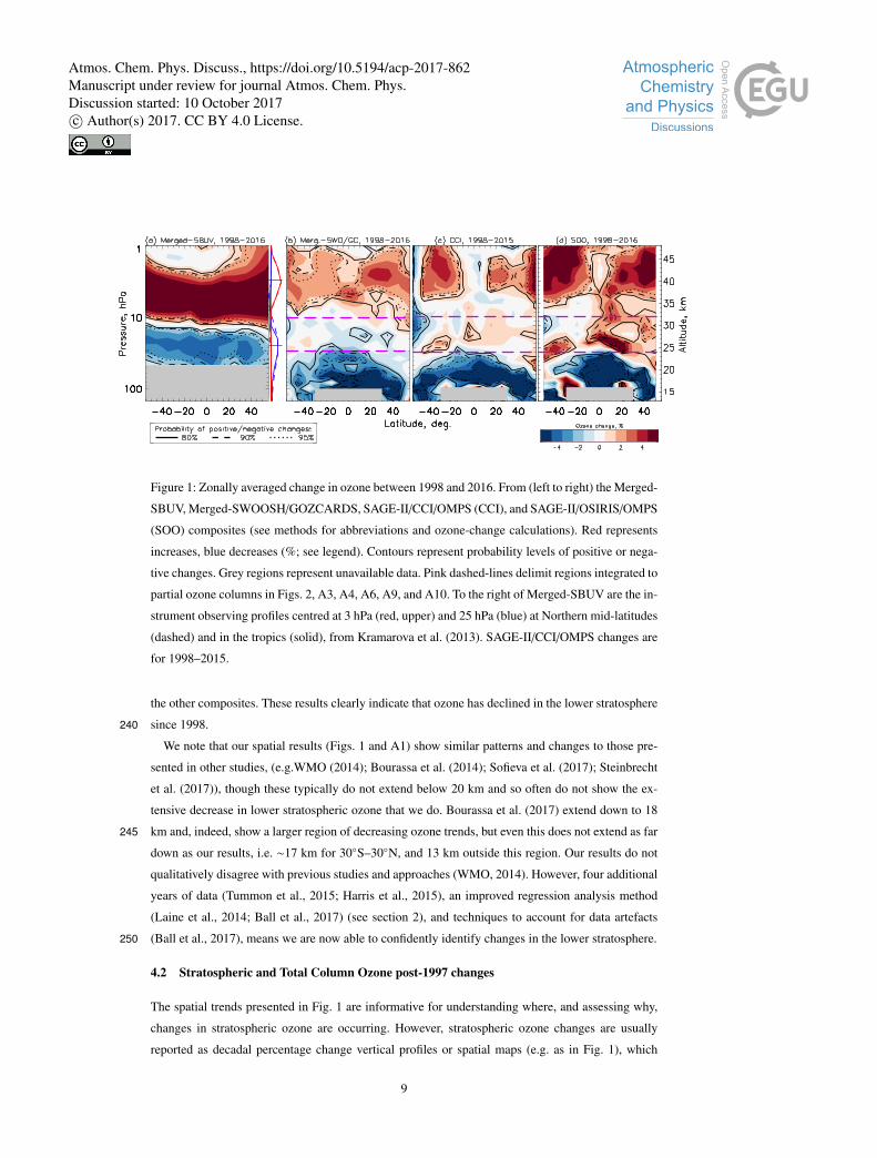
Figure 1: Zonally averaged change in ozone between 1998 and 2016. From (left to right) the Merged-

SBUV, Merged-SWOOSH/GOZCARDS, SAGE-II/CCI/OMPS (CCI), and SAGE-II/OSIRIS/OMPS

(SOO) composites (see methods for abbreviations and ozone-change calculations). Red represents

increases, blue decreases (%; see legend). Contours represent probability levels of positive or nega-

tive changes. Grey regions represent unavailable data. Pink dashed-lines delimit regions integrated to

partial ozone columns in Figs. 2, A3, A4, A6, A9, and A10. To the right of Merged-SBUV are the in-

strument observing profiles centred at 3 hPa (red, upper) and 25 hPa (blue) at Northern mid-latitudes

(dashed) and in the tropics (solid), from Kramarova et al. (2013). SAGE-II/CCI/OMPS changes are

for 1998–2015.

the other composites. These results clearly indicate that ozone has declined in the lower stratosphere

since 1998.240

We note that our spatial results (Figs. 1 and A1) show similar patterns and changes to those pre-

sented in other studies, (e.g.WMO (2014); Bourassa et al. (2014); Sofieva et al. (2017); Steinbrecht

et al. (2017)), though these typically do not extend below 20 km and so often do not show the ex-

tensive decrease in lower stratospheric ozone that we do. Bourassa et al. (2017) extend down to 18

km and, indeed, show a larger region of decreasing ozone trends, but even this does not extend as far245

down as our results, i.e. ∼17 km for 30◦S–30◦N, and 13 km outside this region. Our results do not

qualitatively disagree with previous studies and approaches (WMO, 2014). However, four additional

years of data (Tummon et al., 2015; Harris et al., 2015), an improved regression analysis method

(Laine et al., 2014; Ball et al., 2017) (see section 2), and techniques to account for data artefacts

(Ball et al., 2017), means we are now able to confidently identify changes in the lower stratosphere.250

4.2 Stratospheric and Total Column Ozone post-1997 changes

The spatial trends presented in Fig. 1 are informative for understanding where, and assessing why,

changes in stratospheric ozone are occurring. However, stratospheric ozone changes are usually

reported as decadal percentage change vertical profiles or spatial maps (e.g. as in Fig. 1), which

9


hides the absolute changes in ozone, and the contribution to the total column, which are almost never255

reported. A recovery in the upper stratosphere is important to identify, but this region contributes a

smaller fraction to the total column than the middle and lower stratosphere. Thus, smaller percentage

changes over a reduced altitude range in the lower stratosphere can actually produce larger integrated

changes than in the more extended regions higher up.

In Fig. 2 we present changes in partial column ozone (PCO) in Dobson Units (DU) from Merged-260

SWOOSH/GOZCARDS for the whole stratospheric column (StCO), and for the upper (10–1 hPa),

and lower stratosphere (147–32 hPa or 13–24 km at >30◦; 100–32 hPa or 17–24 km at <30◦), respec-

tively. We note that the tropopause, the boundary layer between the troposphere and stratosphere,

varies seasonally, but is on average around 16 km (tropics) and 10–12 km (mid-latitudes); our con-

servative choice of slightly higher altitudes ensures that we avoid including the troposphere. Due to265

the near-complete temporal and vertical coverage, we focus on the Merged-SWOOSH/GOZCARDS

composite (SAGE-II/OSIRIS/OMPS and SAGE-II/CCI/OMPS are provided in Figs. A3 and A4,

respectively5). Fig. 2 shows posterior distributions of the 1998–2016 ozone changes, with black

numbers representing the percentage of the distribution that is negative, in 10◦ bands (left) and in-

tegrated ‘global’ (defined as 60◦S–60◦N) PCO (right), along with the TCO observed by SBUV (red270

curves and numbers; upper row).

Upper stratospheric ozone (Fig. 2, middle row) has increased since 1998 in almost all latitude

bands, in half the cases at >90% probability, and >95% at 40◦–60◦ in both hemispheres. Globally,

the probability exceeds 99% that upper stratospheric ozone has increased, confirming that the MP

has indeed been successful in reversing trends in this altitude range.275

Changes in the lower stratosphere (Fig. 2, lower row) show ozone decreases, typically exceeding

90% probability (50◦S–50◦N). There is 99% probability that lower stratospheric ozone has decreased

globally (60◦S–60◦N) since 1998; SAGE-II/OSIRIS/OMPS and SAGE-II/CCI/OMPS both support

this result with 87 and 99% probabilities, respectively (Figs. A3 and A4).

Integrating the whole stratosphere vertically, to form the stratospheric column ozone (StCO;280

Fig. 2, upper row), we see that all distributions imply a decrease (i.e. values >50%); probability is

generally higher in tropical latitudes (30◦S–30◦N). Integrating over all latitudes, global StCO (right)

indicates that stratospheric ozone has decreased with >90% probability. We compare the Merged-

SWOOSH/GOZCARDS change with SBUV TCO, the latter of which includes both troposphere and

stratosphere. The global SBUV TCO indicates that ozone has, in contrast to the StCO, changed little285

compared to 1998.

5It should be noted that while each latitude band PCO of SAGE-II/OSIRIS/OMPS and SAGE-II/CCI/OMPS typically has

between 60 and 90% of months where data are available for 1985–2015/6, integrating bands across all latitudes leads to a re-

duction of available months (see Fig. A5), though estimates of the change since 1998 can still be made and uncertainties due to

the reduced data are captured in the posteriors given in Figs. A3 and A4; this does not affect Merged-SWOOSH/GOZCARDS

or SBUV TCO.

10


Figure 2: Merged-SWOOSH/GOZCARDS posterior distributions (shaded) for the 1998–2016 total

and partial column ozone changes. (Top) whole stratospheric column, (middle) upper and (bottom)

lower stratosphere in 10◦ bands for all latitudes (left) and integrated from 60◦S–60◦N (‘Global’,

right). The stratosphere extends deeper at mid-latitudes than equatorial (marked above each latitude).

Numbers above each distribution represents the distribution-percentage that is negative; colours

are graded relative to the percentage-distribution (positive, red-hues, with values <50; negative,

blue). SBUV total column ozone (red curves) is given in the upper row and negative distribution-

percentages are given as red numbers.

We note that uncertainty remains in the middle stratosphere (Fig. A6), with Merged-SWOOSH/GOZCARDS,

SAGE-II/CCI/OMPS, and SAGE-II/OSIRIS/OMPS displaying different changes. SAGE-II/OSIRIS/OMPS,

in particular, shows a significant positive trend, which leads to the global StCO indicating no change

since 1998 (Fig. A3). This is likely a result of how the data were merged to form composites (see290

example in Fig A7 at northern mid-latitudes and 30 km), and is an issue that remains to be resolved

(Harris et al., 2015; Ball et al., 2017; Steinbrecht et al., 2017). Nevertheless, the changes in the up-

per and lower stratosphere are consistent in all ozone composites, and a globally-integrated StCO

decline is indicated by both Merged-SWOOSH/GOZCARDS-O3 and SAGE-II/CCI/OMPS-O3.

11


Figure 3: ‘Global’ 60◦S–60◦N 1985–2016 total (TCO) and partial (PCO) column ozone anomalies.

Deseasonalised and regression model timeseries are given for the Merged-SWOOSH/GOZCARDS

merged composite (grey and black, respectively) for (a) the whole stratospheric column, (b) upper,

(c) middle, and (d) lower stratospheric PCOs. The DLM non-linear trend is the smoothly varying

thick black line. In (a), the deseasonalised SBUV TCO is also given (orange), with the regression

model (red) and the non-linear trend (thick, red). Data are shifted so the trend-line is zero in 1998.

DLM results for WACCM-SD (blue) and SOCOL-SD (purple) from Fig. A11 are also shown.

12


To make these globally-integrated results clear, we show in Fig. 3a the SBUV TCO (yellow/red)295

and Merged-SWOOSH/GOZCARDS StCO (grey/black); in all of the panels in Fig. 3, the timeseries

are bias-shifted so that the smoothly varying non-linear trend crosses the zero line in January 1998,

so that relative changes can be clearly compared. It is interesting to note here that the SBUV TCO

non-linear trend initially increases from 1998, and then peaks in around 2011, before decreasing.

Frith et al. (2014) found similar behaviour when applying linear trend fits to SBUV TCO, fixing the300

start date in January 2000 and incrementally increasing the end date, i.e. the largest positive trend was

found for the period 2000–2011 and thereafter trends decreased. Their analysis ended in 2013, but the

non-linear trend from our DLM analysis, here, shows identical behaviour, and which has continued

decreasing until 2016 and suggests that TCO ozone has now returned to 1998 levels despite an initial

upward trend. Qualitatively similar behaviour is seen in the Merged-SWOOSH/GOZCARDS StCO,305

though less pronounced because of its larger overall downward behaviour (see below, section 4.3),

which lends supporting, independent, evidence that such a turnover in ozone trends might be real.

The StCO from Merged-SWOOSH/GOZCARDS continued to decrease after 1998 and, while this

decline stalled in the late 2000s, since 2012 it has continued to decrease. The overall result is that

StCO is on average lower today than in 1998, by ∼1.5 DU.310

The different stratospheric regimes that contribute to the StCO behaviour can be see in Figs. 3b–d,

where we show, upper, middle (10–32 hPa), and lower stratospheric ozone timeseries from Merged-

SWOOSH/GOZCARDS. A recovery is clear in the upper stratosphere in Fig. 3b, increasing by a

mean of ∼1 DU, and trends have been relatively flat since 1998 in the middle stratosphere (Fig. 3c),

with a mean decrease of ∼ 0.5 DU. However, the result from Merged-SWOOSH/GOZCARDS in the315

lower stratosphere (Fig. 3d) indicates not only that ozone there has declined by ∼2 DU since 1998,

and has been the main contributor to the StCO decrease, but that the lower stratospheric ozone has

seen a continuous and uninterrupted decrease.

4.3 Tropospheric ozone contribution to TCO

The stratosphere accounts for the majority (∼90%) of TCO, so intuitively attribution to TCO changes320

would be expected to come primarily from this region. However, the results in Fig. 2 and 3 suggest a

discrepancy between StCO and TCO. Despite this, there is no serious conflict between the different

changes indicated by global StCO and TCO distributions (Fig. 2) and trends (Fig. 3a), when the

remaining 10% of the TCO, i.e. tropospheric ozone, is considered, as we show in the following.

First, it is important to establish confidence in the SBUV TCO observations. These have been325

very stable since 1998 when comparing SBUV TCO overpass data to the independent ground-based

Arosa TCO observations (Fig. A8). This, therefore, provides confidence in the result that there is

little net change in TCO since 1998. Additionally, Chehade et al. (2014) reported that other TCO

composites agree very well with the SBUV TCO and there is little difference between the various

TCO composites when performing trend analysis.330

13


Figure 4: ‘Global’ 60◦S–60◦N total tropospheric column ozone between 2004 and 2016. OMI/MLS

integrated ozone (grey line) and deseasonalised timeseries (black). The 2005 and 2016 periods are

plotted in blue and red, respectively and the mean and two standard errors on the mean for these two

years are plotted on the right, with the mean value added alongside. The mean linear trend estimate

(dashed line) and the one-standard deviation uncertainty are also provided.

In a second step, we consider global tropospheric ozone changes. In Fig. 4, we present recent esti-

mates from the Aura satellite Ozone Monitoring Instrument and Microwave Limb Sounder (OMI/MLS)

instruments of global (60◦S–60◦N) tropospheric column ozone (TrCO) from 2004 to 2016 (grey),

along with deaseasonalised anomalies (solid black); the deseasonalised years 2005 and 2016 are in-

dicated in blue and red – the means (right) indicate a significant increase in ozone. A linear fit to335

the deseasonalised timeseries indicates an increase in tropospheric ozone of 1.68 DU per decade; if

this has held true for the entire 19 year period (1998–2016) it implies a mean increase of ∼3 DU,

which would more than account for the difference between the StCO and TCO peaks (∼1.6 DU) in

the upper right panel of Fig. 2.

Supporting evidence for tropospheric ozone increases comes from work reconstructing strato-340

spheric ozone changes in a chemistry climate model (CCM). Shepherd et al. (2014) indicates that

tropospheric ozone in the northern (35◦–55◦N) and southern mid-latitudes (35◦–55◦S) may have

increased by ∼1 DU (1998–2011), while equatorial (25◦S–25◦N) may have increased by ∼1.5 DU

respectively. While we consider a longer period, this qualitatively agrees with the latitude-resolved

distributions in Fig. 2, which shows that, except for a couple of southern mid-latitudes (30◦–40◦S and345

50◦–60◦S) and the most northerly band (50◦–60◦N), all TCO posteriors indicate smaller decreases,

or larger increases, compared to the Merged-SWOOSH/GOZCARDS StCO changes.

Returning to the OMI/MLS tropospheric ozone, by separating out TrCO by latitude, and looking at

the mean 2005–2015 change shows significant increases in mean TrCO levels at all latitudes, except

a non-significant increase at 50–60S (see Fig A13). The latitudinal structure and magnitude of the350

TrCO changes, with peaks at ∼30◦ in both hemispheres and clear minima at high latitudes and near

14


the equator, bears resemblance to the piecewise linear post-1998 TCO trends in Fig. 9 of Chehade

et al. (2014) and Fig. 10 of Frith et al. (2014), though there are detailed differences, and so we note

that the difference between StCO and TCO in Fig. 2 does not follow this pattern so coherently, which

may be a result of considering a shorter time period for TrCO, and deserves further consideration.355

OMI/MLS results are not independent from Merged-SWOOSH/GOZCARDS as Aura/MLS forms

a part of this composite post-2005. Nevertheless, OMI/MLS is independent from SBUV TCO; the

OMI TCO component of the product had a drift of less than 1% per decade with respect to SBUV

TCO (McPeters et al., 2015). Regarding OMI, McPeters et al. (2015) stated that the OMI TCO data,

which forms part of the TrCO product when the StCO from Aura/MLS is included, are stable enough360

for ozone trend studies, that OMI has proven to be one of the most stable instruments flown, and they

concluded that OMI provides some of the highest quality ozone data from trend analysis avaliable.

Ziemke and Cooper (2017) found no statistically significant drift with respect to various independent

measures, or between MLS StCO and OMI StCO residuals, but did detect a small drift of +0.5 DU

per decade in OMI/MLS TrCO caused by an error in the OMI total ozone - this was rectified for the365

version we consider here.

A deeper investigation is needed to understand difference in the contributions of TrCO and StCO

to TCO, especially considering uncertainties carefully, but this is beyond the scope of this work.

We note that studies using various data sources show less significant regional increases (and some

decreases) with global estimates ranging from 0.2 to 0.7% per year (∼0.6–2 DU per decade) (Cooper370

et al., 2014; Ebojie et al., 2016; Heue et al., 2016), though these estimates considered different

time periods; this suggests a large range of uncertainty, but even the lower end of the estimated

increases in TrCO are in line with the missing part of the TCO change, after considering StCO,

that we estimate here. Tropospheric ozone is not the main focus of the study here, but the evidence

presented overall suggests the missing component in the declining StCO distributions and trends,375

with respect to constant TCO, is indeed from increasing tropospheric ozone.

4.4 Comparison of stratospheric spatial and partial column ozone trends with models

The observational results for the lower, and whole, stratosphere presented thus far have not been

previously reported. However, it is not clear that this represents a departure from our understanding

of stratospheric trends as presented in modelling studies. We present the percentage ozone change380

from two state-of-the-art chemistry climate models (CCMs) in Fig. 5: (a) the NCAR Community

Earth System Model (CESM) Whole Atmosphere Community Climate Model-4 (WACCM; Marsh

et al. (2013)); and (b) the SOlar Climate Ozone Links (SOCOL; Stenke et al., 2013) model. Both

simulations were performed with the Chemistry Climate Model Initiative phase 1 (CCMI-1) bound-

ary conditions in specified dynamics (SD) mode (see Morgenstern et al. (2017) for information on385

CCMI and boundary conditions used in models). SD uses reanalysis products to constrain model dy-

namics towards observations so as to best represent the dynamics of the atmosphere, while leaving

15


Figure 5: As for Fig. 1, but for (a) WACCM-SD and (b) SOCOL-SD.

chemistry to respond freely to these changes. Such an approach has proven highly accurate at repro-

ducing ozone variability on monthly to decadal timescales in the equatorial upper stratosphere (Ball

et al., 2016). WACCM-SD uses version 1 of the Modern-Era Retrospective analysis for Research and390

Applications (MERRA-1; Rienecker et al. (2011) reanalysis6, while SOCOL-SD uses ERA-Interim

(Dee et al., 2011). Thus, the two models are both independent in terms of how they are constructed,

and the source of nudging fields used, but have similar boundary conditions as prescribed by CCMI-

1.

In Fig. 5 both models display broadly similar behaviour in the upper stratosphere above 10 hPa,395

roughly in line with the observations (Fig. 1). Spatially, in the middle stratosphere there are dif-

ferences in sign, but generally significance is low: WACCM-SD displays broadly positive changes

except in the tropics at 10 and 30 hPa, while SOCOL-SD displays a negative spot centred in the

tropics at 10 hPa, while mid-latitudes are often positive and significant. In the lower stratosphere,

SOCOL-SD displays negative trends in the Southern hemisphere lower stratosphere, but positive400

in the Northern, while WACCM-SD is generally positive everywhere, and significant at the lowest

altitudes, except at 30–40 hPa in the tropics where a negative tendency is seen. In both SOCOL-SD

and WACCM-SD, trends in the lower stratosphere are generally not significant, and do not display

the clear and significant decreases found in the observations. Posterior distributions similar to those

of Fig. 2 are presented for SOCOL-SD and WACCM-SD in Figs. A9 and A10, respectively. The405

6Use of MERRA-2 reanalysis (Gelaro et al., 2017) makes little difference, except in the upper stratosphere after 2004,

where positive trends are larger when using MERRA-2 (see Fig. A12). The WACCM-SD run with MERRA-2 uses CESM

1.2.2 at 1.9×2.5 horizontal resolution and 88 vertical layers up to 140 km, using prescribed aerosols from the RCP 8.5

scenario.

16


displayed behaviour is similar to that described here spatially for the models in Fig. 5, and no sig-

nificant decreases are found (two SOCOL-SD latitude bands display negative changes in the lower

stratosphere with ∼75% probability: 30–40S and 10–20N). It is worth noting that in both cases the

integrated, global trends in the StCO and upper stratosphere are all positive with probabilities of

an increase exceeding 95%, and positive in the lower stratosphere, with 69 and 85% probability410

of an increase in SOCOL-SD and WACCM-SD, respectively. The non-linear DLM trends (Fig. 3)

of WACCM-SD (blue) and SOCOL-SD (purple) emphasize the clearly differing behaviour to the

observations, especially in the lower stratosphere (the deaseasonalised and regression model time-

series are omitted from Fig. 3 for clarity, but provided in Fig. A11). It is worth mentioning that the

behaviour of TCO from the models was similar to SBUV TCO (Fig. 3a) until around 2012, after415

which modelled ozone continued to increase while observations show a gradual decline until 2016

(see discussion in section 4.2).

It is notable that also the suite of CCMVal-2 models, the predecessor of CCMI-1, show little

significant behaviour in the lower stratosphere, with a tendency for positive changes. As shown in

Fig. 2-10 of the WMO (2014) report the ozone trends in the CCMVal-2 multi-model mean from 2000420

to 2013 are positive everywhere except a region bounded by 80–20 hPa and 30S–30N, although only

above ∼10 hPa are trends significant. Furthermore, there is an ozone increase in the mid-latitude

lower stratosphere, albeit non-significant, indicated by the CCMVal-2 models that is not seen in the

observations, suggesting that models may not be simulating that region correctly. Extending to 2016

with two independent nudged models, as shown here, does not change this result, which differs from425

the (i) significant decreases in ozone found in the lower stratosphere, and (ii) the stalled recovery

seen in SBUV TCO while models project continued increases.

Chemistry climate models (CCMs) represent our integrated understanding of processes that gov-

ern ozone variability and trends, and include chemistry, transport and feedbacks on radiation. Over-

all, they capture the historical behaviour in the stratosphere well (e.g. total column ozone trends430

driven by EESC changes). However, when it comes to the UTLS region it is not yet clear if models

do so well. For example, Figs. 7.27 and 7.28 of the CCMVal-2 report SPARC/WMO (2010) indi-

cate a better model performance with respect to UTLS ozone in summer, when transport effects are

weaker and chemistry more important. However, there is a large difference compared to observations

and a wide spread among the models during winter/spring. Transport is affected by many factors,435

e.g. model vertical/horizontal resolution and gravity wave parameterizations, and trends in atmo-

spheric circulation are also hard to measure and, therefore, to assess the models with. Whether the

difference between the models and observations is a result of model design, incorrect boundary con-

ditions (e.g. aerosol contributions from anthropogenic (Yu et al., 2017) or volcanic (Bandoro et al.,

2017) sources may be underestimated), or missing chemistry remains an open question (see below440

for further discussion).

17


5 Conclusions

In summary, we have presented evidence of highly significant changes in stratospheric ozone be-

tween 1998 and 2016. The main findings are that:

(i) the MP is further confirmed to be successfully reducing the impact of hODSs as indicated by445

the highly probable recovery seen in most upper stratospheric (1–10 hPa / 32–48 km) regions

in all composites;

(ii) lower stratospheric ozone (147/100–32 hPa / 13/17–24 km) has continued to decrease since

1998 at all latitudes between 50◦S and 50◦N;

(iii) there are indications that the total, global (60◦S–60◦N) stratospheric ozone may have continued450

to decrease;

(iv) indications of no decrease, or perhaps an increase, in TCO is likely a result of increasing

tropospheric ozone, together with the slowed rate of decrease in stratospheric ozone following

the MP.

(v) state-of-the-art models, nudged to have historical atmospheric dynamics as realistic as possible455

do not reproduce the observed decreases in lower stratospheric ozone, which may suggest

deficiencies in some aspect of the modelling.

The cause for the continuing decline in lower stratospheric ozone is not fully understood and

determining the exact cause is beyond the scope of this study, but there are several possible explana-

tions. CCM simulations indicate that tropical stratospheric ozone is expected to decrease following460

increased upwelling in the tropics (<30◦) linked to an acceleration of the BDC from greenhouse gas

(GHG) induced climate change, which has a larger influence on ozone trends than hODSs in this

region (Randel and Wu, 2007; Oman et al., 2010; WMO, 2014); this may account for some of the

tropical lower stratosphere ozone decrease, but clear evidence for this in observations remains weak

(WMO, 2014). Some modelling and studies also indicate that a rise in the tropopause (Santer et al.,465

2003), due to the warming troposphere, could lead to a localised ozone decrease (Steinbrecht et al.,

1998), though it is not clear of how TCO is affected on large scales, Plummer et al. (2010); Diet-

müller et al. (2014); since the troposphere is continuing to warm, the tropopause may continue rising

and have an affect on stratospheric ozone. We also pose the hypothesis that an acceleration of the

lower stratospheric BDC shallow branch in response to climate change (Randel and Wu, 2007; Oman470

et al., 2010) may more rapidly transport ozone poor air to the mid-latitudes from the tropical lower

stratosphere, where dynamical changes dominate over photochemical ozone production processes

(Johnston, 1975; Perliski et al., 1989). While, these possibilities are dynamically-driven responses

to climate change, a chemically-driven alternative has also been suggested. Observations indicate an

increase in very short lived substances (VSLSs) containing chlorine and bromine species from both475

18


anthropogenic and natural sources (Hossaini et al., 2015). Modelling studies imply that VSLSs pref-

erentially destroy ozone in the lower stratosphere, particularly at mid- and high-latitudes (Hossaini

et al., 2015, 2017). It is thought that these species may delay the restoration of the ozone layer to

pre-1960s levels, but information is available for only a small number of VSLSs and knowledge of

the reaction rate kinetics to determine their impacts is currently not adequate.480

While the reason for the lower stratospheric ozone decline is not yet determined, the signal is clear

and the likely consequences significant. The MP is working, but a reduction in harmful UV radiation

reaching the surface to pre-1980’s levels depends on a restoration of the TCO (WMO, 2014); the

lower stratospheric ozone decline appears to be inhibiting this, and models as yet do not reproduce

these downward trends with significance. Increased transport of ozone into the troposphere from485

the stratosphere is expected if global surface temperatures continue to increase, and may impact air

quality (Hegglin and Shepherd, 2009; Neu et al., 2014); current trends suggest that ozone available

for such exchange is decreasing. Additionally, ozone in the lower stratosphere is an important factor

in radiative forcing (RF) of the climate (Randel and Thompson, 2011), and so far has offset some of

the RF increase from rising GHGs; a reduction in lower stratospheric ozone may lead to reduced RF490

and further offsetting. Finally, the restoration of the ozone layer is essential to reducing the harmful

effects of solar UV radiation on surface life, including humans (Slaper et al., 1996). It is imperative

that we determine the cause of the decline in lower stratospheric ozone identified here, both in order

to predict future changes, and to determine if it is possible to prevent further decreases.

Acknowledgements. GOZCARDS ozone data can be accessed at https://gozcards.jpl.nasa.gov/, SWOOSH at495

http://www.esrl.noaa.gov/csd/groups/csd8/swoosh/, SBUV-MOD and SBUV TCO at http://acd-ext.gsfc.nasa.

gov/Data_services/merged/, and SBUV-MER at ftp://ftp.cpc.ncep.noaa.gov/SBUV_CDR/. W.T.B. and E.V.R.

were funded by the SNSF project 163206 (SIMA). We thank the SPARC LOTUS working group as a forum

for discussion and data exchange. Work at the Jet Propulsion Laboratory was performed under contract with

the National Aeronautics and Space Administration. GOZCARDS ozone data contributions from Ryan Fuller500

(at JPL) are gratefully acknowledged. We are grateful to Daniel Marsh and Doug Kinnison for providing ozone

data from WACCM CESM in specified dynamics mode.

19


References

Ball, W. T., Haigh, J. D., Rozanov, E. V., Kuchar, A., Sukhodolov, T., Tummon, F., Shapiro, A. V., and Schmutz,

W.: High solar cycle spectral variations inconsistent with stratospheric ozone observations, Nature Geo-505

science, 9, 206–209, doi:10.1038/ngeo2640, 2016.

Ball, W. T., Alsing, J., Mortlock, D. J., Rozanov, E. V., Tummon, F., and Haigh, J. D.: Reconciling differences

in stratospheric ozone composites, Atmos. Chem. Phys. Discuss., 2017.

Bandoro, J., Solomon, S., Santer, B. D., Kinnison, D. E., and Mills, M. J.: Detectability of the Impacts of Ozone

Depleting Substances and Greenhouse Gases upon Stratospheric Ozone Accounting for Nonlinearities in510

Historical Forcings, Atmospheric Chemistry and Physics Discussions, 2017, 1–42, doi:10.5194/acp-2017-

585, https://www.atmos-chem-phys-discuss.net/acp-2017-585/, 2017.

Bourassa, A. E., Degenstein, D. A., Randel, W. J., Zawodny, J. M., Kyrölä, E., McLinden, C. A., Sioris, C. E.,

and Roth, C. Z.: Trends in stratospheric ozone derived from merged SAGE II and Odin-OSIRIS satellite

observations, Atmos. Chem. Phys., 14, 6983–6994, doi:10.5194/acp-14-6983-2014, 2014.515

Bourassa, A. E., Roth, C. Z., Zawada, D. J., Rieger, L. A., McLinden, C. A., and Degenstein, D. A.: Drift

corrected Odin-OSIRIS ozone product: algorithm and updated stratospheric ozone trends, Atmos. Meas.

Tech. Discuss., doi:10.5194/amt-2017-229, 2017.

Chehade, W., Weber, M., and Burrows, J. P.: Total ozone trends and variability during 1979-2012 from merged

data sets of various satellites, Atmospheric Chemistry & Physics, 14, 7059–7074, doi:10.5194/acp-14-7059-520

2014, 2014.

Chiodo, G., Marsh, D. R., Garcia-Herrera, R., Calvo, N., and García, J. A.: On the detection of the solar signal

in the tropical stratosphere, Atmospheric Chemistry & Physics, 14, 5251–5269, doi:10.5194/acp-14-5251-

2014, 2014.

Cooper, O. R., Parrish, D. D., Ziemke, J., Balashov, N. V., Cupeiro, M., Galbally, I. E., Gilge, S., Horowitz,525

L., Jensen, N. R., Lamarque, J.-F., Naik, V., Oltmans, S. J., J., S., T., S. D., Thompson, A. M., Thouret, V.,

Wang, Y., and Zbinden, R. M.: Global distribution and trends of tropospheric ozone: An observation-based

review, Elem Sci Anth., p. 29, doi:10.12952/journal.elementa.000029, 2014.

Davis, S. M., Rosenlof, K. H., Hassler, B., Hurst, D. F., Read, W. G., Vömel, H., Selkirk, H., Fujiwara, M., and

Damadeo, R.: The Stratospheric Water and Ozone Satellite Homogenized (SWOOSH) database: a long-term530

database for climate studies, Earth System Science Data, 8, 461–490, doi:10.5194/essd-8-461-2016, 2016.

Dee, D. P., Uppala, S. M., Simmons, A. J., Berrisford, P., Poli, P., Kobayashi, S., Andrae, U., Balmaseda,

M. A., Balsamo, G., Bauer, P., Bechtold, P., Beljaars, A. C. M., van de Berg, L., Bidlot, J., Bormann, N.,

Delsol, C., Dragani, R., Fuentes, M., Geer, A. J., Haimberger, L., Healy, S. B., Hersbach, H., Hólm, E. V.,

Isaksen, L., Kållberg, P., Köhler, M., Matricardi, M., McNally, A. P., Monge-Sanz, B. M., Morcrette, J.-535

J., Park, B.-K., Peubey, C., de Rosnay, P., Tavolato, C., Thépaut, J.-N., and Vitart, F.: The ERA-Interim

reanalysis: configuration and performance of the data assimilation system, Quarterly Journal of the Royal

Meteorological Society, 137, 553–597, doi:10.1002/qj.828, 2011.

Dietmüller, S., Ponater, M., and Sausen, R.: Interactive ozone induces a negative feedback in CO2-

driven climate change simulations, Journal of Geophysical Research (Atmospheres), 119, 1796–1805,540

doi:10.1002/2013JD020575, 2014.

20


Dudok de Wit, T., Bruinsma, S., and Shibasaki, K.: Synoptic radio observations as proxies for upper atmosphere

modelling, Journal of Space Weather and Space Climate, 4, A06, doi:10.1051/swsc/2014003, 2014.

Ebojie, F., Burrows, J. P., Gebhardt, C., Ladstätter-Weißenmayer, A., von Savigny, C., Rozanov, A., Weber, M.,

and Bovensmann, H.: Global tropospheric ozone variations from 2003 to 2011 as seen by SCIAMACHY,545

Atmospheric Chemistry & Physics, 16, 417–436, doi:10.5194/acp-16-417-2016, 2016.

Eyring, V., Cionni, I., Bodeker, G. E., Charlton-Perez, A. J., Kinnison, D. E., Scinocca, J. F., Waugh, D. W.,

Akiyoshi, H., Bekki, S., Chipperfield, M. P., Dameris, M., Dhomse, S., Frith, S. M., Garny, H., Gettel-

man, A., Kubin, A., Langematz, U., Mancini, E., Marchand, M., Nakamura, T., Oman, L. D., Pawson, S.,

Pitari, G., Plummer, D. A., Rozanov, E., Shepherd, T. G., Shibata, K., Tian, W., Braesicke, P., Hardiman,550

S. C., Lamarque, J. F., Morgenstern, O., Pyle, J. A., Smale, D., and Yamashita, Y.: Multi-model assessment

of stratospheric ozone return dates and ozone recovery in CCMVal-2 models, Atmospheric Chemistry &

Physics, 10, 9451–9472, doi:10.5194/acp-10-9451-2010, 2010.

Farman, J. C., Gardiner, B. G., and Shanklin, J. D.: Large losses of total ozone in Antarctica reveal seasonal

ClOx/NOx interaction, Nature, 315, 207–210, doi:10.1038/315207a0, 1985.555

Frith, S. M., Kramarova, N. A., Stolarski, R. S., McPeters, R. D., Bhartia, P. K., and Labow, G. J.: Recent

changes in total column ozone based on the SBUV Version 8.6 Merged Ozone Data Set, Journal of Geophys-

ical Research (Atmospheres), 119, 9735–9751, doi:10.1002/2014JD021889, 2014.

Froidevaux, L., Anderson, J., Wang, H.-J., Fuller, R. A., Schwartz, M. J., Santee, M. L., Livesey, N. J.,

Pumphrey, H. C., Bernath, P. F., Russell, III, J. M., and McCormick, M. P.: Global OZone Chemistry And560

Related trace gas Data records for the Stratosphere (GOZCARDS): methodology and sample results with

a focus on HCl, H2O, and O3, Atmospheric Chemistry & Physics, 15, 10 471–10 507, doi:10.5194/acp-15-

10471-2015, 2015.

Gebhardt, C., Rozanov, A., Hommel, R., Weber, M., Bovensmann, H., Burrows, J. P., Degenstein, D., Froide-

vaux, L., and Thompson, A. M.: Stratospheric ozone trends and variability as seen by SCIAMACHY from565

2002 to 2012, Atmospheric Chemistry & Physics, 14, 831–846, doi:10.5194/acp-14-831-2014, 2014.

Gelaro, R., McCarty, W., Suárez, M. J., Todling, R., Molod, A., Takacs, L., Randles, C. A., Darmenov, A.,

Bosilovich, M. G., Reichle, R., Wargan, K., Coy, L., Cullather, R., Draper, C., Akella, S., Buchard, V.,

Conaty, A., da Silva, A. M., Gu, W., Kim, G.-K., Koster, R., Lucchesi, R., Merkova, D., Nielsen, J. E.,

Partyka, G., Pawson, S., Putman, W., Rienecker, M., Schubert, S. D., Sienkiewicz, M., and Zhao, B.: The570

Modern-Era Retrospective Analysis for Research and Applications, Version 2 (MERRA-2), Journal of Cli-

mate, 30, 5419–5454, doi:10.1175/JCLI-D-16-0758.1, 2017.

Harris, N. R. P., Hassler, B., Tummon, F., Bodeker, G. E., Hubert, D., Petropavlovskikh, I., Steinbrecht, W.,

Anderson, J., Bhartia, P. K., Boone, C. D., Bourassa, A., Davis, S. M., Degenstein, D., Delcloo, A., Frith,

S. M., Froidevaux, L., Godin-Beekmann, S., Jones, N., Kurylo, M. J., Kyrölä, E., Laine, M., Leblanc, S. T.,575

Lambert, J.-C., Liley, B., Mahieu, E., Maycock, A., de Mazière, M., Parrish, A., Querel, R., Rosenlof, K. H.,

Roth, C., Sioris, C., Staehelin, J., Stolarski, R. S., Stübi, R., Tamminen, J., Vigouroux, C., Walker, K. A.,

Wang, H. J., Wild, J., and Zawodny, J. M.: Past changes in the vertical distribution of ozone - Part 3: Analysis

and interpretation of trends, Atmospheric Chemistry & Physics, 15, 9965–9982, doi:10.5194/acp-15-9965-

2015, 2015.580

21


Hegglin, M. I. and Shepherd, T. G.: Large climate-induced changes in ultraviolet index and stratosphere-to-

troposphere ozone flux, Nature Geoscience, 2, 687–691, doi:10.1038/ngeo604, 2009.

Heue, K.-P., Coldewey-Egbers, M., Delcloo, A., Lerot, C., Loyola, D., Valks, P., and van Roozendael, M.:

Trends of tropical tropospheric ozone from 20 years of European satellite measurements and perspectives for

the Sentinel-5 Precursor, Atmospheric Measurement Techniques, 9, 5037–5051, doi:10.5194/amt-9-5037-585

2016, 2016.

Hossaini, R., Chipperfield, M. P., Montzka, S. A., Rap, A., Dhomse, S., and Feng, W.: Efficiency of short-lived

halogens at influencing climate through depletion of stratospheric ozone, Nature Geoscience, 8, 186–190,

doi:10.1038/ngeo2363, 2015.

Hossaini, R., Chipperfield, M. P., Montzka, S. A., Leeson, A. A., Dhomse, S., and Pyle, J. A.: The increasing590

threat to stratospheric ozone from dichloromethane, Nature Communications, 8, doi:10.1038/ncomms15962,

2017.

Johnston, H. S.: Global ozone balance in the natural stratosphere, Reviews of Geophysics and Space Physics,

13, 637–649, doi:10.1029/RG013i005p00637, 1975.

Kramarova, N. A., Bhartia, P. K., Frith, S. M., McPeters, R. D., and Stolarski, R. S.: Interpreting SBUV smooth-595

ing errors: an example using the quasi-biennial oscillation, Atmospheric Measurement Techniques, 6, 2089–

2099, doi:10.5194/amt-6-2089-2013, 2013.

Kyrölä, E., Laine, M., Sofieva, V., Tamminen, J., Päivärinta, S.-M., Tukiainen, S., Zawodny, J., and Thomason,

L.: Combined SAGE II-GOMOS ozone profile data set for 1984-2011 and trend analysis of the vertical

distribution of ozone, Atmospheric Chemistry & Physics, 13, 10 645–10 658, doi:10.5194/acp-13-10645-600

2013, 2013.

Laine, M., Latva-Pukkila, N., and Kyrölä, E.: Analysing time-varying trends in stratospheric ozone time series

using the state space approach, Atmospheric Chemistry & Physics, 14, 9707–9725, doi:10.5194/acp-14-

9707-2014, 2014.

Marsh, D. R. and Garcia, R. R.: Attribution of decadal variability in lower-stratospheric tropical ozone, Geo-605

physical Research Letters, 34, L21807, doi:10.1029/2007GL030935, 2007.

Marsh, D. R., Mills, M. J., Kinnison, D. E., Lamarque, J.-F., Calvo, N., and Polvani, L. M.: Climate Change

from 1850 to 2005 Simulated in CESM1(WACCM), Journal of Climate, 26, 7372–7391, doi:10.1175/JCLI-

D-12-00558.1, 2013.

McPeters, R. D., Bhartia, P. K., Haffner, D., Labow, G. J., and Flynn, L.: The version 8.6 SBUV610

ozone data record: An overview, Journal of Geophysical Research (Atmospheres), 118, 8032–8039,

doi:10.1002/jgrd.50597, 2013.

McPeters, R. D., Frith, S., and Labow, G. J.: OMI total column ozone: extending the long-term data record,

Atmospheric Measurement Techniques, 8, 4845–4850, doi:10.5194/amt-8-4845-2015, 2015.

Molina, M. J. and Rowland, F. S.: Stratospheric sink for chlorofluoromethanes: chlorine atomc-atalysed de-615

struction of ozone, Nature, 249, 810–812, doi:10.1038/249810a0, 1974.

Morgenstern, O., Hegglin, M. I., Rozanov, E., O’Connor, F. M., Abraham, N. L., Akiyoshi, H., Archibald,

A. T., Bekki, S., Butchart, N., Chipperfield, M. P., Deushi, M., Dhomse, S. S., Garcia, R. R., Hardiman,

S. C., Horowitz, L. W., Jöckel, P., Josse, B., Kinnison, D., Lin, M., Mancini, E., Manyin, M. E., Marchand,

M., Marécal, V., Michou, M., Oman, L. D., Pitari, G., Plummer, D. A., Revell, L. E., Saint-Martin, D.,620

22


Schofield, R., Stenke, A., Stone, K., Sudo, K., Tanaka, T. Y., Tilmes, S., Yamashita, Y., Yoshida, K., and Zeng,

G.: Review of the global models used within phase 1 of the Chemistry-Climate Model Initiative (CCMI),

Geoscientific Model Development, 10, 639–671, doi:10.5194/gmd-10-639-2017, 2017.

Nair, P. J., Froidevaux, L., Kuttippurath, J., Zawodny, J. M., Russell, J. M., Steinbrecht, W., Claude, H., Leblanc,

T., van Gijsel, J. A. E., Johnson, B., Swart, D. P. J., Thomas, A., Querel, R., Wang, R., and Anderson, J.: Sub-625

tropical and midlatitude ozone trends in the stratosphere: Implications for recovery, Journal of Geophysical

Research (Atmospheres), 120, 7247–7257, doi:10.1002/2014JD022371, 2015.

NCAR: The Climate Data Guide: Multivariate ENSO Index, Retrieved from https://climatedataguide.ucar.edu/

climate-data/multivariate-enso-index, 2013.

Neu, J. L., Flury, T., Manney, G. L., Santee, M. L., Livesey, N. J., and Worden, J.: Tropospheric ozone variations630

governed by changes in stratospheric circulation, Nature Geoscience, 7, 340–344, doi:10.1038/ngeo2138,

2014.

Newman, P. A., Daniel, J. S., Waugh, D. W., and Nash, E. R.: A new formulation of equivalent effective strato-

spheric chlorine (EESC), Atmospheric Chemistry & Physics, 7, 4537–4552, 2007.

Oman, L. D., Plummer, D. A., Waugh, D. W., Austin, J., Scinocca, J. F., Douglass, A. R., Salawitch, R. J.,635

Canty, T., Akiyoshi, H., Bekki, S., Braesicke, P., Butchart, N., Chipperfield, M. P., Cugnet, D., Dhomse, S.,

Eyring, V., Frith, S., Hardiman, S. C., Kinnison, D. E., Lamarque, J.-F., Mancini, E., Marchand, M., Michou,

M., Morgenstern, O., Nakamura, T., Nielsen, J. E., Olivié, D., Pitari, G., Pyle, J., Rozanov, E., Shepherd,

T. G., Shibata, K., Stolarski, R. S., TeyssèDre, H., Tian, W., Yamashita, Y., and Ziemke, J. R.: Multimodel

assessment of the factors driving stratospheric ozone evolution over the 21st century, Journal of Geophysical640

Research (Atmospheres), 115, D24306, doi:10.1029/2010JD014362, 2010.

Perliski, L. M., London, J., and Solomon, S.: On the interpretation of seasonal variations of stratospheric ozone,

Journal of Geophysical Research, 37, 1527–1538, doi:10.1016/0032-0633(89)90143-8, 1989.

Plummer, D. A., Scinocca, J. F., Shepherd, T. G., Reader, M. C., and Jonsson, A. I.: Quantifying the contribu-

tions to stratospheric ozone changes from ozone depleting substances and greenhouse gases, Atmospheric645

Chemistry & Physics, 10, 8803–8820, doi:10.5194/acp-10-8803-2010, 2010.

Randel, W. J. and Thompson, A. M.: Interannual variability and trends in tropical ozone derived from SAGE

II satellite data and SHADOZ ozonesondes, Journal of Geophysical Research (Atmospheres), 116, D07303,

doi:10.1029/2010JD015195, 2011.

Randel, W. J. and Wu, F.: A stratospheric ozone profile data set for 1979-2005: Variability, trends, and650

comparisons with column ozone data, Journal of Geophysical Research (Atmospheres), 112, D06313,

doi:10.1029/2006JD007339, 2007.

Rienecker, M. M., Suarez, M. J., Gelaro, R., Todling, R., Bacmeister, J., Liu, E., Bosilovich, M. G., Schubert,

S. D., Takacs, L., Kim, G.-K., Bloom, S., Chen, J., Collins, D., Conaty, A., da Silva, A., Gu, W., Joiner,

J., Koster, R. D., Lucchesi, R., Molod, A., Owens, T., Pawson, S., Pegion, P., Redder, C. R., Reichle, R.,655

Robertson, F. R., Ruddick, A. G., Sienkiewicz, M., and Woollen, J.: MERRA: NASA’s Modern-Era Retro-

spective Analysis for Research and Applications, Journal of Climate, 24, 3624–3648, doi:10.1175/JCLI-D-

11-00015.1, 2011.

23


Santer, B. D., Wehner, M. F., Wigley, T. M. L., Sausen, R., Meehl, G. A., Taylor, K. E., Ammann, C., Arblaster,

J., Washington, W. M., Boyle, J. S., and Brüggemann, W.: Contributions of Anthropogenic and Natural660

Forcing to Recent Tropopause Height Changes, Science, 301, 479–483, doi:10.1126/science.1084123, 2003.

Scarnato, B., Staehelin, J., Stübi, R., and Schill, H.: Long-term total ozone observations at Arosa (Switzerland)

with Dobson and Brewer instruments (1988-2007), Journal of Geophysical Research (Atmospheres), 115,

D13306, doi:10.1029/2009JD011908, 2010.

Shepherd, T. G., Plummer, D. A., Scinocca, J. F., Hegglin, M. I., Fioletov, V. E., Reader, M. C., Remsberg,665

E., von Clarmann, T., and Wang, H. J.: Reconciliation of halogen-induced ozone loss with the total-column

ozone record, Nature Geoscience, 7, 443–449, doi:10.1038/ngeo2155, 2014.

Sioris, C. E., McLinden, C. A., Fioletov, V. E., Adams, C., Zawodny, J. M., Bourassa, A. E., Roth, C. Z., and

Degenstein, D. A.: Trend and variability in ozone in the tropical lower stratosphere over 2.5 solar cycles

observed by SAGE II and OSIRIS, Atmospheric Chemistry & Physics, 14, 3479–3496, doi:10.5194/acp-14-670

3479-2014, 2014.

Slaper, H., Velders, G. J. M., Daniel, J. S., de Gruijl, F. R., and van der Leun, J. C.: Estimates of ozone de-

pletion and skin cancer incidence to examine the Vienna Convention achievements, Nature, 384, 256–258,

doi:10.1038/384256a0, 1996.

Sofieva, V., Kyrölä, E., Laine, M., Tamminen, J., Degenstein, D., Bourassa, A., Roth, C., Zawada, D., Weber,675

M., Rozanov, A., Rahpoe, N., Stiller, G., Laeng, A., von Clarmann, T., Walker, K., Sheese, P., Hubert, D.,

van Roozendael, M., Zehner, C., Damadeo, R., Zawodny, J., Kramarova, N., , and Bhartia, P.: Merged SAGE

II, Ozone_cci and OMPS ozone profiles dataset and evaluation of ozone trends in the stratosphere, Atmos.

Chem. Phys. Discuss., doi:10.5194/acp-2017-598, 2017.

Sofieva, V. F., Kalakoski, N., Päivärinta, S.-M., Tamminen, J., Laine, M., and Froidevaux, L.: On sampling680

uncertainty of satellite ozone profile measurements, Atmospheric Measurement Techniques, 7, 1891–1900,

doi:10.5194/amt-7-1891-2014, 2014.

Solomon, S., Ivy, D. J., Kinnison, D., Mills, M. J., Neely, R. R., and Schmidt, A.: Emergence of healing in the

Antarctic ozone layer, Science, 353, 269–274, doi:10.1126/science.aae0061, 2016.

SPARC/WMO: SPARC Report on the Evaluation of Chemistry-Climate Models, SPARC, 2010.685

Steinbrecht, W., Claude, H., KöHler, U., and Hoinka, K. P.: Correlations between tropopause height

and total ozone: Implications for long-term changes, Journal of Geophysical Research, 103, 19,

doi:10.1029/98JD01929, 1998.

Steinbrecht, W., Froidevaux, L., Fuller, R., Wang, R., Anderson, J., Roth, C., Bourassa, A., Degenstein, D.,

Damadeo, R., Zawodny, J., Frith, S., McPeters, R., Bhartia, P., Wild, J., Long, C., Davis, S., Rosenlof, K.,690

Sofieva, V., Walker, K., Rahpoe, N., Rozanov, A., Weber, M., Laeng, A., von Clarmann, T., Stiller, G.,

Kramarova, N., Godin-Beekmann, S., Leblanc, T., Querel, R., Swart, D., Boyd, I., Hocke, K., Kämpfer,

N., Maillard Barras, E., Moreira, L., Nedoluha, G., Vigouroux, C., Blumenstock, T., Schneider, M., Garcìa,

O., Jones, N., Mahieu, E., Smale, D., Kotkamp, M., Robinson, J., Petropavlovskikh, I., Harris, N., Hassler,

B., Hubert, D., and Tummon, F.: An update on ozone profile trends for the period 2000 to 2016, Atmos.695

Chem. Phys. Discuss., 2017, 1–24, doi:10.5194/acp-2017-391, https://www.atmos-chem-phys-discuss.net/

acp-2017-391/, 2017.

24


Stenke, A., Schraner, M., Rozanov, E., Egorova, T., Luo, B., and Peter, T.: The SOCOL version 3.0 chemistry-

climate model: description, evaluation, and implications from an advanced transport algorithm, Geoscientific

Model Development, 6, 1407–1427, doi:10.5194/gmd-6-1407-2013, 2013.700

Tegtmeier, S., Hegglin, M. I., Anderson, J., Bourassa, A., Brohede, S., Degenstein, D., Froidevaux, L.,

Fuller, R., Funke, B., Gille, J., Jones, A., Kasai, Y., Krüger, K., Kyrölä, E., Lingenfelser, G., Lumpe, J.,

Nardi, B., Neu, J., Pendlebury, D., Remsberg, E., Rozanov, A., Smith, L., Toohey, M., Urban, J., Clar-

mann, T., Walker, K. A., and Wang, R. H. J.: SPARC Data Initiative: A comparison of ozone climatolo-

gies from international satellite limb sounders, Journal of Geophysical Research (Atmospheres), 118, 12,705

doi:10.1002/2013JD019877, 2013.

Thomason, L., Ernest, N., Millan, L., Rieger, L., Bourassa, A., Vernier, J., Peter, T., Luo, B., and Arfeuille, F.:

A global, space-based stratospheric aerosol climatology: 1979 to 2016, Earth Syst. Sci. Data, in preparation,

doi:10.5067/GloSSAC-L3-V1.0, 2017.

Tiao, G. C., Xu, D., Pedrick, J. H., Zhu, X., and Reinsel, G. C.: Effects of autocorrelation and temporal sampling710

schemes on estimates of trend and spatial correlation, Journal of Geophysical Research, 95, 20 507–20 517,

doi:10.1029/JD095iD12p20507, 1990.

Tummon, F., Hassler, B., Harris, N. R. P., Staehelin, J., Steinbrecht, W., Anderson, J., Bodeker, G. E., Bourassa,

A., Davis, S. M., Degenstein, D., Frith, S. M., Froidevaux, L., Kyrölä, E., Laine, M., Long, C., Penckwitt,

A. A., Sioris, C. E., Rosenlof, K. H., Roth, C., Wang, H.-J., and Wild, J.: Intercomparison of vertically re-715

solved merged satellite ozone data sets: interannual variability and long-term trends, Atmospheric Chemistry

& Physics, 15, 3021–3043, doi:10.5194/acp-15-3021-2015, 2015.

Vigouroux, C., Blumenstock, T., Coffey, M., Errera, Q., García, O., Jones, N. B., Hannigan, J. W., Hase, F.,

Liley, B., Mahieu, E., Mellqvist, J., Notholt, J., Palm, M., Persson, G., Schneider, M., Servais, C., Smale,

D., Thölix, L., and De Mazière, M.: Trends of ozone total columns and vertical distribution from FTIR720

observations at eight NDACC stations around the globe, Atmospheric Chemistry & Physics, 15, 2915–2933,

doi:10.5194/acp-15-2915-2015, 2015.

Wild, J. D. and Long, C. S.: A Coherent Ozone Profile Dataset from SBUV, SBUV/2: 1979 to 2016, in prepa-

ration, 2017.

WMO: Scientific Assessment of Ozone Depletion: 2010, Global Ozone Research and Monitoring Project, 52,725

516, 2011.

WMO: Scientific Assessment of Ozone Depletion: 2014 Global Ozone Research and Monitoring Project Re-

port, World Meteorological Organization, p. 416, geneva, Switzerland, 2014.

WMO/NASA: International Ozone Trends Panel Report, Report, 1988.

Yu, P., Rosenlof, K. H., Liu, S., Telg, H., Thornberry, T. D., Rollins, A. W., Portmann, R. W., Bai, Z., Ray,730

E. A., Duan, Y., Pan, L. L., Toon, O. B., Bian, J., and Gao, R.-S.: Efficient transport of tropospheric aerosol

into the stratosphere via the Asian summer monsoon anticyclone, Proceedings of the National Academy of

Science, 114, 6972–6977, doi:10.1073/pnas.1701170114, 2017.

Ziemke, J. R. and Cooper, O. R.: Tropospheric ozone, in State of the Climate in 2016, Bull. Amer. Meteorol.,

in press, 2017.735

Ziemke, J. R., Chandra, S., Duncan, B. N., Froidevaux, L., Bhartia, P. K., Levelt, P. F., and Waters, J. W.: Tropo-

spheric ozone determined from Aura OMI and MLS: Evaluation of measurements and comparison with the

25


Figure A1: 1998-2016 ozone change. As for Fig. 1; from left to right, SWOOSH, GOZCARDS,

SBUV-NOAA, and SBUV-NASA composites.

Figure A2: Example of merging result for SWOOSH and GOZCARDS. The result of merging pro-

cedure detailed in Ball et al. (2017) applied to GOZCARDS (dark blue), SWOOSH (light-blue)

ozone composites in the 0-10◦N band at four pressure levels indicated in the top right of each panel.

The resulting Merged-SWOOSH/GOZCARDS timeseries is shown as a dashed-black line with two

standard deviation uncertainty in grey shading.

Global Modeling Initiative’s Chemical Transport Model, Journal of Geophysical Research (Atmospheres),

111, D19303, doi:10.1029/2006JD007089, 2006.

26


Figure A3: SAGE-II/OSIRIS/OMPS posterior distributions for the 1998-2016 ozone changes. See

caption of Fig. 2 for details.

27


Figure A4: SAGE-II/CCI/OMPS posterior distributions for the 1998-2015 ozone changes. See cap-

tion of Fig. 2 for details.

28


Figure A5: The fraction of data available for the (top) StCO/TCO, (middle) upper stratosphere, and

(bottom) lower stratosphere posterior estimates in Figs. 2, A3, and A4. Global (right) are much lower

in SAGE-II/OSIRIS/OMPS and SAGE-II/CCI/OMPS because if data are missing in any latitude in

a particular month, the global PCO or StCO is assigned no data.

29


Figure A6: Posterior distributions in the middle stratosphere for the 1998-2015/2016 ozone changes.

Similar to panels in Fig. 2, but for the middle stratosphere (32-10 hPa, ∼24-32 km) for (top) Merged-

SWOOSH/GOZCARDS, (middle) SAGE-II/CCI/OMPS, and (bottom) SAGE-II/OSIRIS/OMPS.

30


Figure A7: SAGE-II/OSIRIS/OMPS (red) and SAGE-II/CCI/OMPS (black) at northern mid-

latitudes at 30 km. (Upper) The deseasonalised changes relative to 2005–2013, and (lower) SAGE-

II/OSIRIS/OMPS minus SAGE-II/CCI/OMPS. Approximate dates when OSIRIS and OMPS were

introduced into the composites are shown with vertical red lines, before/after which a shift in the

mean appears.

Figure A8: Ozone over Arosa, Switzerland, 1970-2016. (a) Absolute ozone from SBUV Total Col-

umn Ozone (TCO) overpass observations (red) compared to the ground-based Arosa TCO obser-

vations (black), with Arosa shifted to the SBUV mean for 1998-2013; (b) as for (a) with the sea-

sonal cycle removed; (c) the monthly difference between timeseries in (b) and a 24-month Gaussian

smoothing (thick line).

31


Figure A9: SOCOL-SD posterior distributions for the 1998-2015 ozone changes. See caption of

Fig. 2 for details.

32


Figure A10: WACCM-SD posterior distributions for the 1998-2014 ozone changes. See caption of

Fig. 2 for details.

33


Figure A11: As for Fig. 3, but with deseasonalised and regression model timeseries from

SOCOL-SD (purple) and WACCM-SD (blue). DLM results for SBUV-TCO and Merged-

SWOOSH/GOZCARDS are retained in this plot from Fig 3; see Fig 3 for more details.

34


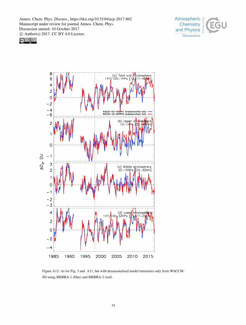
Figure A12: As for Fig. 3 and A11, but with deseasonalised model timeseries only from WACCM-

SD using MERRA-1 (blue) and MERRA-2 (red).

35


Figure A13: Mean and two standard errors of tropical column ozone (TrCO) change between 2005

and 2016 from OMI/MLS. The upper panel shows the absolute levels in 10◦ latitude bins in 2005

(blue) and 2016 (red), while the lower panel gives the difference between 2005 and 2016 with com-

bined errors, similar to the right panel of Fig. 4.

36


continuous decline in lower stratospheric ozone sets · pdf filecontinuous decline in lower...

Documents