Context-based Context-based adaptive binary adaptive binary

arithmetic coding in arithmetic coding in the H.264/AVC video the H.264/AVC video

compressioncompression

IEEE CSVT July 2003IEEE CSVT July 2003

Detlev Marpe, Heiko Schwarz, and Thomas Detlev Marpe, Heiko Schwarz, and Thomas WiegandWiegand

2003/11/042003/11/04

Presented by Chen-hsiu HuangPresented by Chen-hsiu Huang

CABAC

OutlineOutline• Introduction• The CABAC framework• Detailed description of CABAC• Experimental result• Conclusion

Past deficienciesPast deficiencies• Entropy coding such as MPEG-2, H.263, MPEG-4

(SP) is based on fixed tables of VLCs.• Due to VLCs, coding events with probability > 0.5

cannot be efficiently represented. • The usage of fixed VLC tables does not allow an

adaptation to the actual symbol statistics.• Since there is a fixed assignment of VLC tables

and syntax elements, existing inter-symbol redundancies cannot be exploited.

Why?

SolutionsSolutions• The first hybrid block-based video coding

schemes that incorporate an adaptive binary arithmetic coder was presented in [6].

• The first standard that use arithmetic entropy coder is given by Annex E of H.263 [4].

• However, the major drawbacks contains:– Annex E is applied to the same syntax elements as the

VLC elements of H.263.– All the probability models an non-adaptive that their

underlying probability as assumed to be static.– The generic m-ary arithmetic coder used involves a

considerable amount of computational complexity.

Jump!

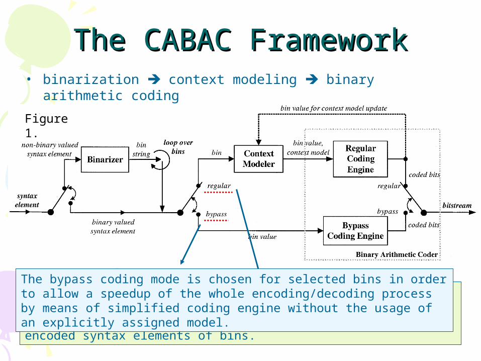
The CABAC FrameworkThe CABAC Framework• binarization context modeling binary arithmetic coding

In the regular coding mode, each bin enters the context modeling stage, where a probability model is selected such that the corresponding choice may depend on previously encoded syntax elements of bins.

The bypass coding mode is chosen for selected bins in order to allow a speedup of the whole encoding/decoding process by means of simplified coding engine without the usage of an explicitly assigned model.

Figure 1.

BinarizationBinarization• Consider the value “3” of mb_type, which signals the

macroblock type “P_8x8”, is given by “001”.• The symbol probability p(“3”) is equal to the product of p(C0)

(“0”), p(C1)(“0”), and p(C2)(“1”), where C0, C1, and C2 are denote the binary probability models of the internal nodes.

Figure 2.

Back

• Adaptive m-ary binary arithmetic coding (m > 2) is in general requiring at least two multiplication for each symbol to encode as well as a number of fairly operations to perform the probability update [36].

• Contrary, fast, multiplication-free variants of binary arithmetic coding, one of which was specifically developed for the CABAC frame, as described below.

• Since the probability of symbols with larger bin strings is typically very low, the computation overhead in fairly small and can be easily compensated by using a fast binary coding engine.

• Finally, binarization enables context modeling on sub-symbol level. For the most frequently observed bins, conditional probability can be used, while less frequently observed bins can be treaded using a joint, typically zero-order probability model.

Why?

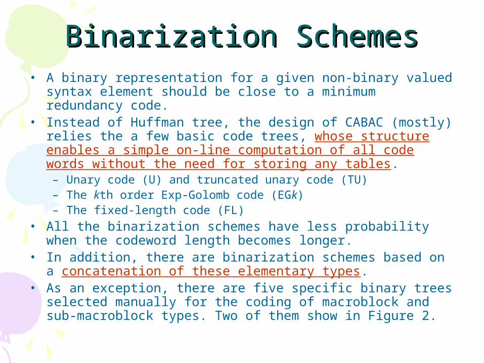
Binarization SchemesBinarization Schemes• A binary representation for a given non-binary valued

syntax element should be close to a minimum redundancy code.

• Instead of Huffman tree, the design of CABAC (mostly) relies the a few basic code trees, whose structure enables a simple on-line computation of all code words without the need for storing any tables.– Unary code (U) and truncated unary code (TU)– The kth order Exp-Golomb code (EGk)– The fixed-length code (FL)

• All the binarization schemes have less probability when the codeword length becomes longer.

• In addition, there are binarization schemes based on a concatenation of these elementary types.

• As an exception, there are five specific binary trees selected manually for the coding of macroblock and sub-macroblock types. Two of them show in Figure 2.

Unary and Truncated Unary Unary and Truncated Unary BinarizationBinarization

• For each unsigned integer valued symbol x >= 0, the unary code word in CABAC consists if x “1” bits plus a terminating “0” bit.

• The truncated unary (TU) code is only defined for x with 0 <= x <= S, where for x < S the code is given by the unary code, whereas for x=S the terminating “0” bit is neglected.

• For example:– U: 5 => 111110– TU with S=9:

• 6: => 1111110• 9: => 111111111

kkth order Exp-Golomb Binarizationth order Exp-Golomb Binarization• The prefix part of the EGk codeword consists of a

unary code corresponding to the value l(x)=floor(log2(x/2k+1))

• The EGk suffix part is computed as the binary representation of x+2k(1-2l(x)) using k+l(x) significant bits.

Fixed-Length BinarizationFixed-Length Binarization• Let x denote a given value of such a syntax

element, where 0 <= x <= S. Then, the FL codeword of x is simply given by the binarization representation of x with a fixed (minimum) number lFL=ceil(log2S) of bits.

• Typically, FL binarization is applied to syntax elements with a nearly uniform distribution or to syntax elements, where each bit in the FL binary representation represents a specific coding decisions.– E.g. In the part of the coded block pattern symbol

related to the luminance residual data.

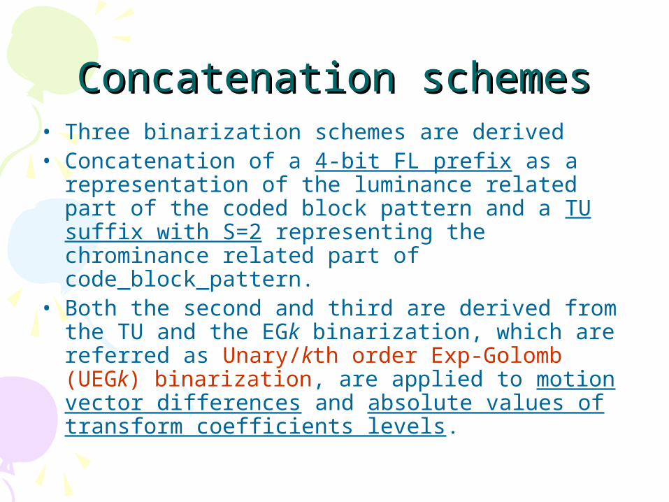
Concatenation schemesConcatenation schemes• Three binarization schemes are derived• Concatenation of a 4-bit FL prefix as a

representation of the luminance related part of the coded block pattern and a TU suffix with S=2 representing the chrominance related part of code_block_pattern.

• Both the second and third are derived from the TU and the EGk binarization, which are referred as Unary/kth order Exp-Golomb (UEGk) binarization, are applied to motion vector differences and absolute values of transform coefficients levels.

• The design of these concatenated binarization scheme is motivated by the following observations:– First, the unary code is the simplest prefix-free code in

terms of implementation cost.– Second, it permits a fast adaptation of the individual

symbol probabilities in the sub-sequent context modeling stage, since the arrangement of the nodes in the corresponding tree is typically such that with increasing distance of the internal nodes from the root node the corresponding binary probabilities are less skewed.

• These observations are only accurate for small values of the absolute motion vector differences and transform coefficient levels. For larger values, there is not much use of an adaptive modeling leading to the idea of concatenating and adaptation.

E.g. E.g. mvdmvd, motion vector difference, motion vector difference• For the prefix part of the UEGk bin string, a TU

binarization with a cutoff S=9 is involed for min(|mvd|, 9). – If mvd is equal to zero, the bin string consists only the

prefix codeword “0”.

• If the condition |mvd| >= 9 holds, the suffix in constructed as an EG3 codeword for the value of |mvd| - 9, to which the sign of mvd is appended using the sign bit “1” for a negative mvd and “0” otherwise. For mvd values with 0 < |mvd| < 9, the suffix consists only of the sign bit.

• With the choice of the Exp-Golomb parameter k=3, the suffix code words are given such that a geometrical increase of the prediction error in units of two samples is captured by a linear increase in the corresponding suffix code word length.

Figure 3.

UEG0 binarization for encoding of absolution values of transform coefficient levels.

Context modelingContext modeling• Suppose a pre-defined set T of past symbols, a so-called

context template, and a related set C={0,…,C-1} of contexts is given, where the context are specified by a modeling function F:TC operating on the template T.

• For each symbol x to be code, a conditional probability p(x|F(z)) is estimated by switching between different probability models according to the already coded neighboring symbols z in T. Thus, p(x|F(z)) is estimated on the fly by tracking the actual source statistics.

• The number τ of different conditional probabilities to be estimated for an alphabet size of m is equal to τ=C(m-1).

• This implies that by increasing the number of C, there is a point where overfitting of the model may occur.

• In CABAC, only very limited context templates T consisting of a few neighboring of the current symbol to encode are employed such that only a small number of different context models C is used.

• Second, context modeling is restricted to select bins of the binarized symbols. As a result, the model cost is drastically reduced.

• Four basic design types of context models can be distinguished in CABAC. The first type involves a context template with up to two neighboring syntax elements in the past of the current syntax element to encode.

Figure 4. illustration of a context template consisting of two neighboring syntax element A and B to the left and on top of the current syntax element C.

Types of context modelingTypes of context modeling• The second type of current is only defined for the syntax

elements of mb_type and sub_mb_type. • For this kind of context models, the values of prior coded

bins (b0,b1,...,bi-1) are used for the choice of a model for a given bin with index i.

Note that in CABAC these context models are only used to select different models for different internal nodes of the corresponding binary trees.

Figure 2.

•Both the third and fourth type of context models is applied to residual data only. In contrast to all other types of context models, both types depend on the context categories of different block types.

•The third type does not rely on past coded data, but on the position in the scanning path.

– Significant map

•The fourth type, modeling functions are specified that involve the evaluation of the accumulated number of encoded/decoded levels with a specific value prior to the current level bin to encode/decode.

– Level information

Context index Context index γγ•The entity of probability

models used in CABAC can be arranged in a linear fashion called context index γ.

•Each probability model relate to a given context index γ is determined by two values, a 6-bit probability state index αγ and the (binary) βγ of the most probable symbol (MPS).

•(αγ βγ,) for 0≤ γ ≤398 represented as 7-bit unsigned integer. Figure 5. syntax elements and

associated range of context indices

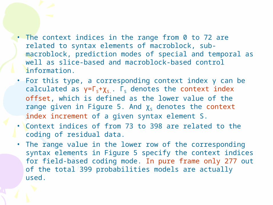
• The context indices in the range from 0 to 72 are related to syntax elements of macroblock, sub-macroblock, prediction modes of special and temporal as well as slice-based and macroblock-based control information.

• For this type, a corresponding context index γ can be calculated as γ=ΓS+χS.. ΓS denotes the context index offset, which is defined as the lower value of the range given in Figure 5. And χS denotes the context index increment of a given syntax element S.

• Context indices of from 73 to 398 are related to the coding of residual data.

• The range value in the lower row of the corresponding syntax elements in Figure 5 specify the context indices for field-based coding mode. In pure frame only 277 out of the total 399 probabilities models are actually used.

•For other syntax elements of residual data, a context index γ is given by: γ=ΓS+ΔS(ctx_cat)+χS. Here the context category (ctx_cat) dependent offset ΔS is employed. (Figure 6)

•Note that only past coded value of syntax elements are evaluated that belong to the same slice, where the current coding process takes place.

Figure 6. Basic types with number of coefficients and associated context categories.

Back

Binary arithmetic codingBinary arithmetic coding• Binary arithmetic is based on the principal of recursive

interval subdivision.

• Suppose that an estimate of the probability pLPS in (0,0.5] of the least probable symbol (LPS) is given and its lower bound L and its width R. Based on this, the given interval is sub-divided into two sub-intervals: RLPS=R•pLPS (3), and the dual interval is RMPS=R-RLPS.

• In a practical implementation, the main bottleneck in terms of throughput is the multiplication operation required.

• A significant amount of work has been published aimed at speeding up the required calculation by introducing some approximations of either the range R or of the probability pLPS such that multiplication can be avoided. [32-34]

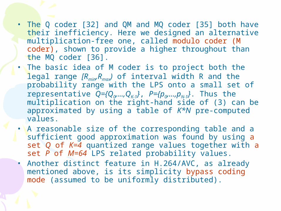
• The Q coder [32] and QM and MQ coder [35] both have their inefficiency. Here we designed an alternative multiplication-free one, called modulo coder (M coder), shown to provide a higher throughout than the MQ coder [36].

• The basic idea of M coder is to project both the legal range [Rmin,Rmax) of interval width R and the probability range with the LPS onto a small set of representative Q={Q0,...,QK-1}, P={p0,...,pN-1}. Thus the multiplication on the right-hand side of (3) can be approximated by using a table of K*N pre-computed values.

• A reasonable size of the corresponding table and a sufficient good approximation was found by using a set Q of K=4 quantized range values together with a set P of M=64 LPS related probability values.

• Another distinct feature in H.264/AVC, as already mentioned above, is its simplicity bypass coding mode (assumed to be uniformly distributed).

Details of CABACDetails of CABAC• The syntax elements are divided into two

categories.– The first contains elements related to macroblock type,

sub-macroblock type, and information of prediction modes both of spatial and of temporal type as well as slice and macroblock-based control information.

– In the second, all residual data elements, i.e., all syntax elements related to the coding of transform coefficients are combined.

• In addition, a more detailed explanation of the probability estimation process and the table-based binary arithmetic coding engine of CABAC is given.

Coding of macroblock type, prediction Coding of macroblock type, prediction mode, and control informationmode, and control information

• At the top level of the macroblock layer syntax the signaling of mb_skip_flag and mb_type is performed. The binary-valued mb_skip_flag indicates whether the current macroblock in a P/SP or B slice is skipped.

• For a given macroblock C, the related context models involves the mb_skip_flag values of the neighboring A at left and B on top. Given by:– χMbSkip(C) = (mb_skip_flag(A) != 0) ? 0: 1 + (mb_skip_flag(B) != 0) ?

0: 1

• If one or both of the neighboring A or B are not available, the mb_skip_type (C) value is set to 0.

Macroblock typeMacroblock type• As already stated above. Figure 2 shows the

binarization trees for mb_type and sub_mb_type that are used in P/SP slices.

• Note the mb_type value of “4” for P slices is not used in CABAC entropy coding mode. For the values “5”-”30” of mb_type, which is further specified in [1].

• For coding a bin value corresponding to the binary decision at an internal node shown in Figure 2, separate context models denote by C0,...,C3 for mb_type and C’0,...,C’3 for sub_mb_type are employed.

Figure 2

Coding of prediction modesCoding of prediction modes• Intra prediction modes for luma 4x4: the

luminance intra prediction modes for 4x4 blocks are itself predicted resulting in the syntax elements of the binary-values prev_intra4x4_pred_mode_flag and rem_intra4x4_pred_mode, where the latter is only present if the former takes a value of 0.

• For coding these syntax elements, two separate probability models are utilized: one for coding of the flag and another for coding each bin value of the 3-FL binarization value of rem_intra4x4_pred_mode.

• Intra prediction modes for chroma:

– χChPerd(C) = (ChPredInDcMode(A) != 0) ? 0: 1 + (ChPredInDcMode(B) != 0) ? 0: 1

• Reference Picture Index:

– χRefIdx(C) = (RefIdxZeroFlag(A) != 0) ? 0: 1 + 2× ((RefIdxZeroFlag(B) != 0) ? 0: 1)

• Components of motion vector differences:– mvd(X,cmp) denote the value of a motion vector

difference component of direction cmp in {hori, vert} related to a macroblock or sub-macroblock partition X.

• Macroblock-based quantization parameter change: – For updating the quantization parameter on a

macroblock level, mb_qp_delta is present for each non-skipped macroblock. For coding the signed value δ(C) of this syntax element, δ(C) is first mapped onto a positive value by

– δ+(C)=2| δ (C)|-((δ(C)>0) ? 1: 0)– Then δ+(C) is binarized using the unary binarization

scheme. • End of slice flag:

– For signaling the last macroblock (macroblock pair) in a slice, the end_of_slice_flag is present for each macroblock (pair).

– The event of non-terminating macroblock is related to the highest possible MPS possibility

• Macroblock pair field flag:– χMbField(C) = mb_field_decoding_flag(A) + mb_field_decoding_flag(B)

Coding of residual dataCoding of residual data• A one-bit symbol coded_block_flag and a binary-

valued significant map are used to indicate the occurrence and the location of non-zero transform coefficients in a given block.

• Non-zero levels are encoded in reverse scanning order.

• Context models for coding of nonzero transform coefficients are chosen based on the number of previously transmitted nonzero levels within the reverse scanning path.

• First the coded block flag is transmitted for the given block of transform coefficients unless the coded block pattern or the macroblock mode indicated that the regarded block has no nonzero coefficients.

• If the coded block flag is nonzero, a significant map specifying the position of significant coefficients is encoded.

• Finally, the absolute value of the level as well as the sign is encoded for each significant transform coefficient. Figure 7.

• Coded block pattern: For each non-skipped macroblock with prediction mode not equal to intra_16x16, the coded_block_pattern symbol indicates which of the six 8x8 blocks – four luminance and two chrominance – contain nonzero transform coefficients.

• A given value of the syntax element coded_block_pattern is binarized using the concatenation of a 4-bit FL and a TU binarization with cutoff value S=2.

• Coded block flag: is a one-bit symbol, which indicate if there are significant, i.e. nonzero coefficients inside single block of transform coefficients.

• Scanning of transform coefficients: the 2-D array of transform coefficient levels of those sub-blocks for which the coded_block_flag indicates nonzero entries are first mapped onto a 1D list using a given scanning pattern.

Encoding process of residual dataEncoding process of residual data

• Significance map: If the significant_coeff_flag symbol is one, a further one-bit symbol last_significant_coefficient is sent. This symbol indicates if the current significant coefficient is the last in inside the block or if further significant coefficients follow.

• Level information: The value of significant coefficients (levels) are encoded by using two coding symbols: coeff_abs_level_minus1, and coeff_sign_flag. The UEG0 binarization scheme is used for encoding of coeff_abs_level_minus1.

• The levels are transmitted in reverse scanning order allowing the usage of reasonable adjust context models.

• Context modes for residual data: In H.264/AVC, there 12 types of transform coefficient blocks, which typically have different kinds of statistics. To keep the number of different context models small, they are classified into five categories as in Figure 6.

• For each of these categories, a special set of context models is used for all syntax elements related to residual data.

• coded_block_pattern: For bin indices from 0 to 3 corresponding to the four 8x8 luminance blocks, – χCBP(C,bin_idx) = ((CBP_Bit(A) != 0) ? 0: 1) +

2*((CBP_Bit(B) != 0) ? 0: 1)• For indices 4 and 5, are specified in [1]

Figure 6

Context models for residual dataContext models for residual data

• Coded Block Flag: Coding of the coded_block_flag utilizes four different probability models for each of the five categories as specified in Figure 6.– χCBFlag(C) = coded_block_flag(A) + 2*coded_block_flag(B)

• Significant map: For encoding the significant map, up to 15 different probability models are used for both significant_coeff_flag and last_significant_flag.– The choice of the models and the context index

increments depend on the scanning position– χSIG(coeff[i]) = χLAST(coeff[i]) = i

• Level information: Reverse scanning of the level information allows a more reliable estimation of the statistics, because at the end of the scanning path it is very likely to observe the occurrence of successive so-called trailing 1’s.

Probability estimationProbability estimation• For CABAC, 64 representative probability values

pσ in [0.01875, 0.5] were derived for the LPS by:– Pσ=α* Pσ-1 for all σ=1,...,63

– α=(0.01875 / 0.5)^(1/63) and p0=0.5Figure 8. LPS probability values and transition rules for updating the probability estimation of each state after observing a LPS (dashed lines in left direction) and a MPS (solid lines in right direction).

• Both the chosen scaling factor α ≈ 0.95 and the cardinality N=64 of the set probabilities represent a good compromise between the desire for fast adaptation (α 0, small N) and sufficiently stable and accurate estimate (α 1, large N).

• As a result of this design, each context model in CABAC can be completely determined by two parameters: its current estimate of the LPS probability and its value of MPS β being either 0 or 1.

• Actually, for a given probability state, the update depends on the state index and the value of the encoded symbol identified either as a LPS or a MPS.

• The derivation of the transition rules for the LPS probability is based on the following relation between a given LPS probability pold and its updated counterpart pnew:

Table-based binary arithmetic Table-based binary arithmetic codingcoding

• Actually, the CABAC coding engine consists of two sub-engines, one for regular coding mode and the other for bypass coding engine.

• Interval sub-division in regular coding mode: The internal state of the arithmetic encoding engine is as usual characterized by two quantities: the current interval R and the base L of the current code interval.

Figure 9.

• First, the current interval R is approximated by a quantized value Q(R), using an equi-partition of the whole range 28≤R<29 into four cells. But instead of using the corresponding representative quantized values Q0, Q1, Q2, and Q3. Q(R) is only addressed by its quantizer index ρ, e.g. ρ=(R>>6) & 3.

• Thus, this index and the probability state index are used as entries in a 2D table TabRangeLPS to determine (approximate) the LPS related sin-interval range RLPS. Here the table TabRangeLPS contains all 64x4 pre-computed product values pσ․Qρ for 0≤σ≤63, and 0≤ ρ≤3 in 8 bit precision.

• Bypass coding mode: To speed up the encoding/decoding of symbols, for which R-RLPS ≈RLPS ≈R/2 is assumed to hold.

• The variable L is doubled before choosing the lower or upper sub-interval depending on the value of the symbol to encode (0 or 1).

• In this way, doubling of L and R in the sub-sequent renormalization in the bypass is operated with doubled decision threshold.

Figure 10.

• Renormalization and carry-over control: A renormalization operation after interval sub-division is required whenever the new interval range R no longer stays with its legal range of [28,29).

• For the CABAC engine, the renormalization process and carry-over control of [37] was adopted.

• This implies, in particular, that the encoder has to resolve any carry propagation by monitoring the bits that are outstanding for being emitted.

• More details can be found in [1].

Experimental resultExperimental result• In our experiments, we compare the coding efficiency of

CABAC to the coding efficiency of the baseline entropy coding method of H.264/AVC. The baseline entropy coding method uses the zero-order Exp-Golomb code for all syntax elements with the exception of the residual data, which are coded using the coding method of CAVLC [1], [2].

• For the range of acceptable video quality for broadcast application of about 30–38 dB and averaged over all tested sequences, bit-rate savings of 9% to 14% are achieved, where higher gains are obtained at lower rates.

ReferencesReferences• [1] “Draft ITU-T Recommendation H.264 and Draft ISO/IEC 14 496-10 AVC,"

in Joint Video Team of ISO/IEC JTC1/SC29/WG11 & ITU-T SG16/Q.6 Doc. JVT-G050, T. Wieg, Ed., Pattaya, Thailand, Mar. 2003.

• [2] T. Wiegand, G. J. Sullivan, G. Bjontegaard, and A. Luthra, “Overview of the H.264/AVC Video Coding Standard,” IEEE Trans. Circuits Syst. Video Technol., vol. 13, pp. 560–576, July 2003.

• [4] “Video Coding for Low Bitrate Communications, Version 1,” ITU-T, ITU-T Recommendation H.263, 1995.

• [6] C. A. Gonzales, “DCT Coding of Motion Sequences Including Arithmetic Coder,” ISO/IEC JCT1/SC2/WP8, MPEG 89/187, MPEG 89/187, 1989.

• [32] W. B. Pennebaker, J. L. Mitchell, G. G. Langdon, and R. B. Arps, “An overview of the basic principles of the Q-coder adaptive binary arithmetic coder,” IBM J. Res. Dev., vol. 32, pp. 717–726, 1988.

• [33] J. Rissanen and K. M. Mohiuddin, “A multiplication-free multialphabet arithmetic code,” IEEE Trans. Commun., vol. 37, pp. 93–98, Feb. 1989.

• [34] P. G. Howard and J. S. Vitter, “Practical implementations of arithmetic coding,” in Image and Text Compression, J. A. Storer, Ed. Boston, MA: Kluwer, 1992, pp. 85–112.

• [36] D. Marpe and T.Wiegand, “A highly efficient multiplication-free binary arithmetic coder and its application in video coding,” presented at the IEEE Int. Conf. Image Proc. (ICIP), Barcelona, Spain, Sept. 2003.

Back

Q1.Q1.• The problem with this scheme lies in the fact that Huffman

codes have to be an integral number of bits long.• The optimal number of bits to be used for each symbol is

the -log2(1/p), where p is the probability of a given character. • Thus, if the probability of a character is 1/256, such as

would be found in a random byte stream, the optimal number of bits per character is log base 2 of 256, or 8.

• If the probability goes up to 1/2, the optimum number of bits needed to code the character would go down to 1.

• If a statistical method can be developed that can assign a 90% (> 0.5) probability to a given character, the optimal code size would be 0.15 bits. The Huffman coding system would probably assign a 1 bit code to the symbol, which is 6 times longer than is necessary.

Back

Q2.Q2. Back

For each symbol to encode, the upper bound u(u) and low bound l(l) of the interval containing the tag for the sequence must be computed.

)()(

)1()()1()1()1()(

)1()1()1()(

nXnnnn

nXnnnn

xFlulu

xFlull

H.264 / MPEG-4 Part 10 : Introduction to CABAC

• When entropy_coding_mode is set to 1, an arithmetic coding system is used to encode and decode H.264 syntax elements.

• The arithmetic coding scheme selected for H.264, Context-based Adaptive Binary Arithmetic Coding or CABAC, achieves good compression performance through – Selecting probability models for each syntax

element according to the element’s context, – Adapting probability estimates based on local

statistics and – Using arithmetic coding.

Coding stagesCoding stages• Binarization

– CABAC uses Binary Arithmetic Coding which means that only binary decisions (1 or 0) are encoded.

– A non-binary-valued symbol (e.g. a transform coefficient or motion vector) is "binarized" or converted into a binary code prior to arithmetic coding.

– This process is similar to the process of converting a data symbol into a variable length code but the binary code is further encoded (by the arithmetic coder) prior to transmission.

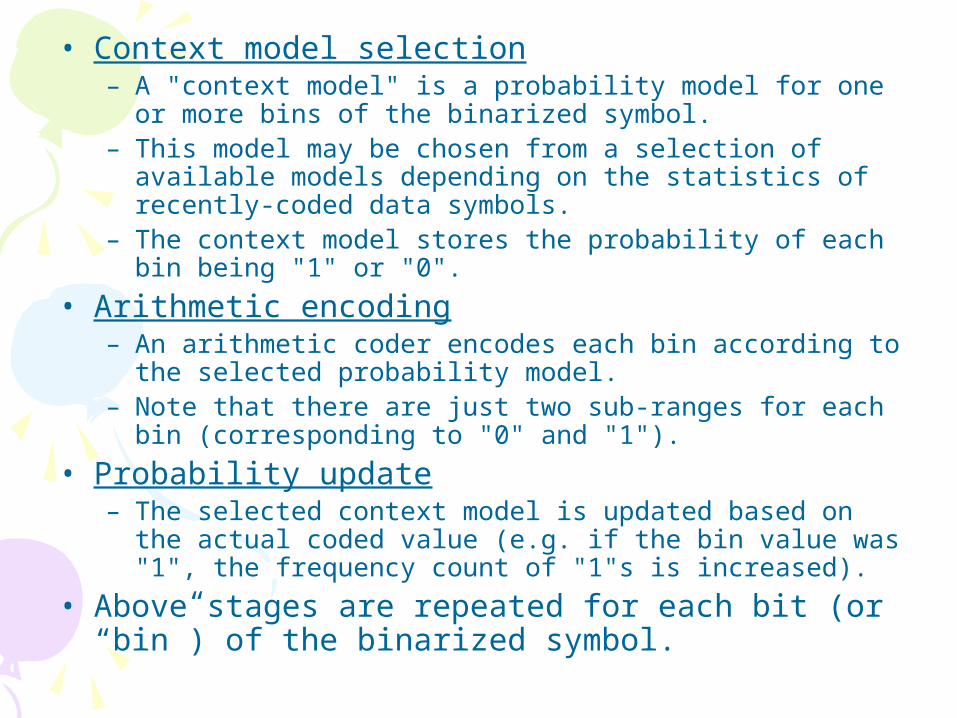
• Context model selection– A "context model" is a probability model for one or more

bins of the binarized symbol. – This model may be chosen from a selection of available

models depending on the statistics of recently-coded data symbols.

– The context model stores the probability of each bin being "1" or "0".

• Arithmetic encoding– An arithmetic coder encodes each bin according to the

selected probability model. – Note that there are just two sub-ranges for each bin

(corresponding to "0" and "1").

• Probability update– The selected context model is updated based on the

actual coded value (e.g. if the bin value was "1", the frequency count of "1"s is increased).

• Above stages are repeated for each bit (or “bin”) of the binarized symbol.

The coding processThe coding process•Binarization. We will

illustrate the coding process for one example, MVDx (motion vector difference in the x-direction).

– Binarization is carried out according to the following table for |MVDx|<9 (larger values of MVDx are binarized using an Exp-Golomb codeword).

•(Note that each of these binarized codewords are uniquely decodeable).

|MVDx| Binarization

0 0

1 10

2 110

3 1110

4 11110

5 111110

6 1111110

7 11111110

8 111111110

• Choose a context model for each bin. One of 3 models is selected for bin 1, based on previous coded MVD values. The L1 norm of two previously-coded values, ek, is calculated:

– ek=|MVDA|+|MVDB|

– A: left block, B: above block

• If ek is small, then there is a high probability that the current MVD will have a small magnitude; if ek is large then it is more likely that the current MVD will have a large magnitude. We select a probability table (context model) accordingly.

ekContext model for bin 1

0 <= ek < 3 Model 0

3 <= ek < 32 Model 1

32 <= ek Model 2

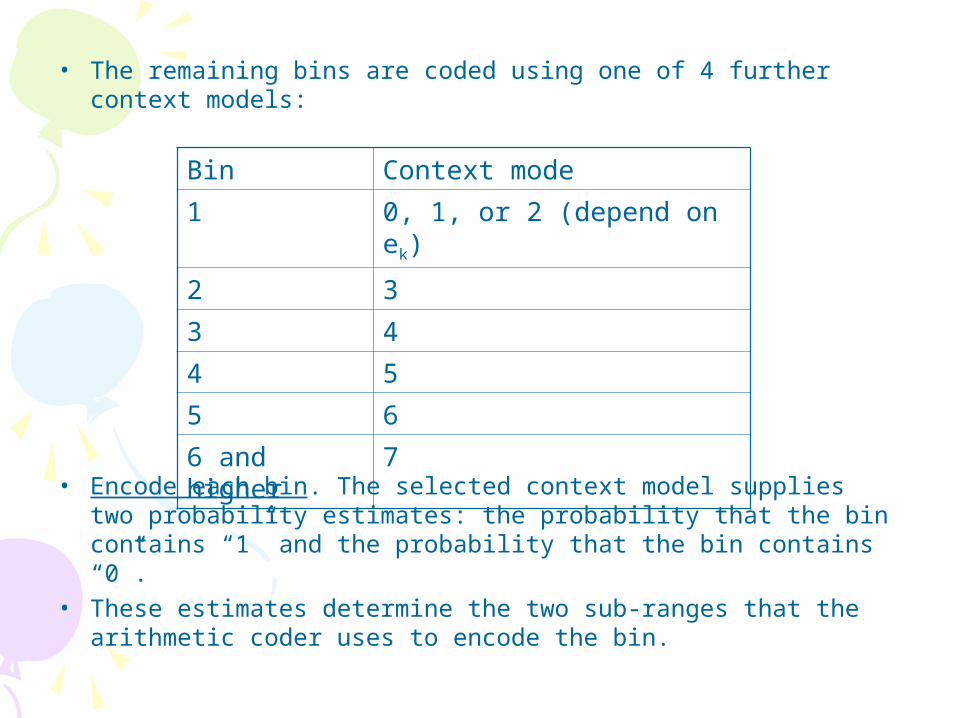
• The remaining bins are coded using one of 4 further context models:

• Encode each bin. The selected context model supplies two probability estimates: the probability that the bin contains “1” and the probability that the bin contains “0”.

• These estimates determine the two sub-ranges that the arithmetic coder uses to encode the bin.

Bin Context mode

1 0, 1, or 2 (depend on ek)

2 3

3 4

4 5

5 6

6 and higher 7

• Update the context models. For example, if context model 2 was selected for bin 1 and the value of bin 1 was “0”, the frequency count of “0”s is incremented. This means that the next time this model is selected, the probability of an “0” will be slightly higher.

• When the total number of occurrences of a model exceeds a threshold value, the frequency counts for “0” and “1” will be scaled down, which in effect gives higher priority to recent observations.

• At the beginning of each coded slice, the context models are initialized depending on the initial value of the Quantization Parameter QP (since this has a significant effect on the probability of occurrence of the various data symbols).

The arithmetic coding engineThe arithmetic coding engine• The arithmetic decoder has three distinct

properties:– Probability estimation is performed by a transition

process between 64 separate probability states for “Least Probable Symbol” (LPS, the least probable of the two binary decisions “0” or “1”).

– The range R representing the current state of the arithmetic coder is quantized to a small range of pre-set values before calculating the new range at each step, making it possible to calculate the new range using a look-up table (i.e. multiplication-free).

– A simplified encoding and decoding process is defined for data symbols with a near-uniform probability distribution. (bypass)

• The definition of the decoding process is designed to facilitate low-complexity implementations of arithmetic encoding and decoding.

Back