Construction and Refinement of PreferenceOrdered Decision Classes

Hoang Nhat Dau1, Salem Chakhar2,3, Djamila Ouelhadj1,3 andAhmed M. Abubahia4

1 Department of Mathematics, Faculty of Technology, University of Portsmouth, UKnhat.dau@myport.ac.uk, djamila.ouelhadj@port.ac.uk

2 Portsmouth Business School, University of Portsmouth, UKsalem.chakhar@port.ac.uk

3 Centre for Operational Research & Logistics, University of Portsmouth, UK4 School of Computing, Faculty of Technology, University of Portsmouth, UK

ahmed.abubahia@port.ac.uk

Abstract. Preference learning methods are commonly used in multicri-teria analysis. The working principle of these methods is similar to classi-cal machine learning techniques. A common issue to both machine learn-ing and preference learning methods is the difficulty of the definition ofdecision classes and the assignment of objects to these classes, especiallyfor large datasets. This paper proposes two procedures permitting to au-tomatize the construction of decision classes. It also proposes two simplerefinement procedures, that rely on the 80-20 principle, permitting tomap the output of the construction procedures into a manageable set ofdecision classes. The proposed construction procedures rely on the mostelementary preference relation, namely dominance relation, which avoidsthe need for additional information or distance/(di)similarity functions,as with most of existing clustering methods. Furthermore, the simplic-ity of the 80-20 principle on which the refinement procedures are based,make them very adequate to large datasets. Proposed procedures areillustrated and validated using real-world datasets.

Keywords: Clustering, Preference learning, Classification, Classes con-struction

1 Introduction

Preference learning methods [3][12] are commonly used in multicriteria analysis.These methods are often used to build a preference model based on a sampleof past decisions for further prescriptive decision purposes. Preference learningmethods have been inspired by knowledge discovery techniques and preferencemodeling methods. The working principle of preference learning methods is sim-ilar to classical machine learning methods [10]: they use a subset of data, calledlearning set, to extract some knowledge permitting to classify unseen objects. Incontrary to machine learning approaches, preference learning methods assumethat both attributes and decision classes are preference-ordered.

2 H.N. Dau et al.

The definition of the learning set is a crucial step in the application of ma-chine and preference learning methods [1][11]. It involves two operations: (i) theselection of a representative subset of objects, and (ii) their assignment into dif-ferent pre-defined decision classes. A common issue to both to machine learningand preference learning methods is the difficulty of defining the decision classes.The situation is further complicated especially for large datasets.

One possible solution to define the learning set is to use one of existing mul-ticriteria ordered clustering methods e.g. [2][4][5][6][7][14]. However, these meth-ods are very demanding in terms of additional information (such as preferenceparameters) and require the specification of a distance/(di)similarity functions.

In this paper, we propose two procedures automatizing the construction ofdecision classes. These procedures permit to reduce the cognitive effort requiredfrom the decision maker and then extend the application domain of preferencelearning methods. We also propose two simple 80-20 principle-based refinementprocedures that permit to map the output of the construction procedures into amanageable set of decision classes.

The rest of the paper goes as follows. Section 2 provides the background.Sections 3 and 4 present the construction and refinement procedures, and Section5 illustrates them using a real-world dataset. Section 6 concludes the paper.

2 Background

2.1 Problem Description

Let U be a non-empty finite set of objects and Q is a non-empty finite setof attributes such that q : U → Vq for every q ∈ Q. The Vq is the domain ofattribute q, V =

⋃q∈Q Vq, and f : U×Q→ V is the information function defined

such that f(x, q) ∈ Vq for each attribute q and object x ∈ U . The value f(x, q)corresponds to the evaluation of object x on attribute q ∈ Q. The domains ofcondition attributes are supposed to be ordered according to a decreasing orincreasing preference. Such attributes are often called criteria.

The objective is to partition U into a finite number of preference-ordereddecision classes Cl = {Clt, t ∈ T}, T = {1, · · · , n}, such that each x ∈ U belongsto one and only one class.

2.2 Dominance Relation and Graph

The dominance relation ∆ is defined for each pair of objects x and y as follows:

x∆y ⇔ f(x, q) ≥ f(y, q),∀q ∈ Q. (1)

This definition applies for gain-type (i.e. benefit) criteria. For cost-type cri-teria, the symbol ‘≥’ should be replaced with ‘≤’. Equation (1) implements theweak version of the dominance relation since all the inequality are large. Clearly,this version of dominance relation is reflexive (i.e. x∆x, x ∈ U) and transitive(i.e. if x∆y and y∆z, then x∆z, ∀x, y, z ∈ U) (but in general not complete).

Construction and Refinement of Preference Ordered Decision Classes 3

Consequently, it defines a partial preorder on U . The strict version of the dom-inance relation ∆s requires at least one strict inequality in Equation (1). Thestrict dominance relation is no longer reflexive but still transitive. It is easy tosee that ∆s ⊆ ∆ (i.e. x∆sy ⇒ x∆y, ∀x, y ∈ U).

The dominance relations on U ×U can be summarized through a dominancematrix M [xij ]h× h where h = |U |, i.e. the number of objects in U and

xij =

{1, If xi∆xj ,0, Otherwise.

(2)

The dominance relation defines a partial preorder on the objects set U . Anypreorder can be represented by a directed graph, with elements of the set cor-responding to vertices, and the order relation between pairs of elements cor-responding to the directed edges between vertices. Therefore, the dominancerelation can be represented as directed graph G = (U,E) with elements U cor-responding to vertices, and the dominance relation between pairs of elementscorresponding to the directed edges E between vertices, defined as E = {(x, y) ∈U × U : x∆y}. The graph G is constructed using a top-to-bottom order. Thismeans that if a node x dominates a node y, x appears above y in the graph.

2.3 Running Example

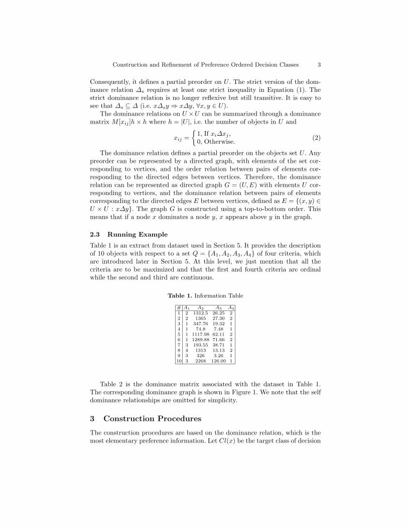
Table 1 is an extract from dataset used in Section 5. It provides the descriptionof 10 objects with respect to a set Q = {A1, A2, A3, A4} of four criteria, whichare introduced later in Section 5. At this level, we just mention that all thecriteria are to be maximized and that the first and fourth criteria are ordinalwhile the second and third are continuous.

Table 1. Information Table

# A1 A2 A3 A4

1 2 1312.5 26.25 22 2 1365 27.30 23 1 347.76 19.32 14 1 74.8 7.48 15 1 1117.98 62.11 26 1 1289.88 71.66 27 3 193.55 38.71 18 4 1313 13.13 29 3 326 3.26 110 3 2268 126.00 1

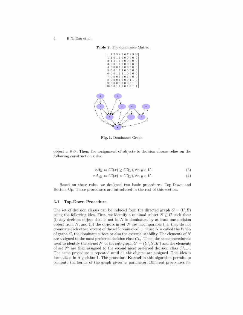
Table 2 is the dominance matrix associated with the dataset in Table 1.The corresponding dominance graph is shown in Figure 1. We note that the selfdominance relationships are omitted for simplicity.

3 Construction Procedures

The construction procedures are based on the dominance relation, which is themost elementary preference information. Let Cl(x) be the target class of decision

4 H.N. Dau et al.

Table 2. The dominance Matrix

1 2 3 4 5 6 7 8 9 101 1 0 1 1 0 0 0 0 0 02 1 1 1 1 0 0 0 0 0 03 0 0 1 1 0 0 0 0 0 04 0 0 0 1 0 0 0 0 0 05 0 0 1 1 1 0 0 0 0 06 0 0 1 1 1 1 0 0 0 07 0 0 0 1 0 0 1 0 0 08 0 0 0 1 0 0 0 1 1 09 0 0 0 0 0 0 0 0 1 010 0 0 1 1 0 0 1 0 1 1

Fig. 1. Dominance Graph

object x ∈ U . Then, the assignment of objects to decision classes relies on thefollowing construction rules:

x∆y ⇔ Cl(x) ≥ Cl(y),∀x, y ∈ U. (3)

x∆sy ⇔ Cl(x) > Cl(y),∀x, y ∈ U. (4)

Based on these rules, we designed two basic procedures: Top-Down andBottom-Up. These procedures are introduced in the rest of this section.

3.1 Top-Down Procedure

The set of decision classes can be induced from the directed graph G = (U,E)using the following idea. First, we identify a minimal subset N ⊆ U such that:(i) any decision object that is not in N is dominated by at least one decisionobject from N ; and (ii) the objects in set N are incomparable (i.e. they do notdominate each other, except of the self dominance). The set N is called the kernelof graph G, the dominant subset or also the external stability. The elements of Nare assigned to the most preferred decision class Cln. Then, the same procedure isused to identify the kernel N ′ of the sub-graph G′ = (U \N,E′) and the elementsof set N ′ are then assigned to the second most preferred decision class Cln−1.The same procedure is repeated until all the objects are assigned. This idea isformalized in Algorithm 1. The procedure Kernel in this algorithm permits tocompute the kernel of the graph given as parameter. Different procedures for

Construction and Refinement of Preference Ordered Decision Classes 5

computing a Kernel of graph are available in the literature [8][9]. Algorithm 1runs in O(β|U |) where β is the complexity of computing the kernel.

Algorithm 1: TopDown ProcedureInput : S = 〈U,Q, V, f〉, // information table.Output: Cl, // equivalence classes.

1 n←− |U |;2 Z ←− ∅;3 while (Z 6= U) do4 E ←− {(x, y) : x, y ∈ U \ Z and x∆y};5 G←− (U \ Z,E);6 Cln ←− Kernel(G);7 Z ←− Z ∪ Cln;8 n←− n− 1;

9 re-label decision classes Cl|U|, · · · , Cln+1 as Cl|U|−n, · · · , Cl1;

10 Cl←− {Cl1, · · · , Cln};11 return Cl;

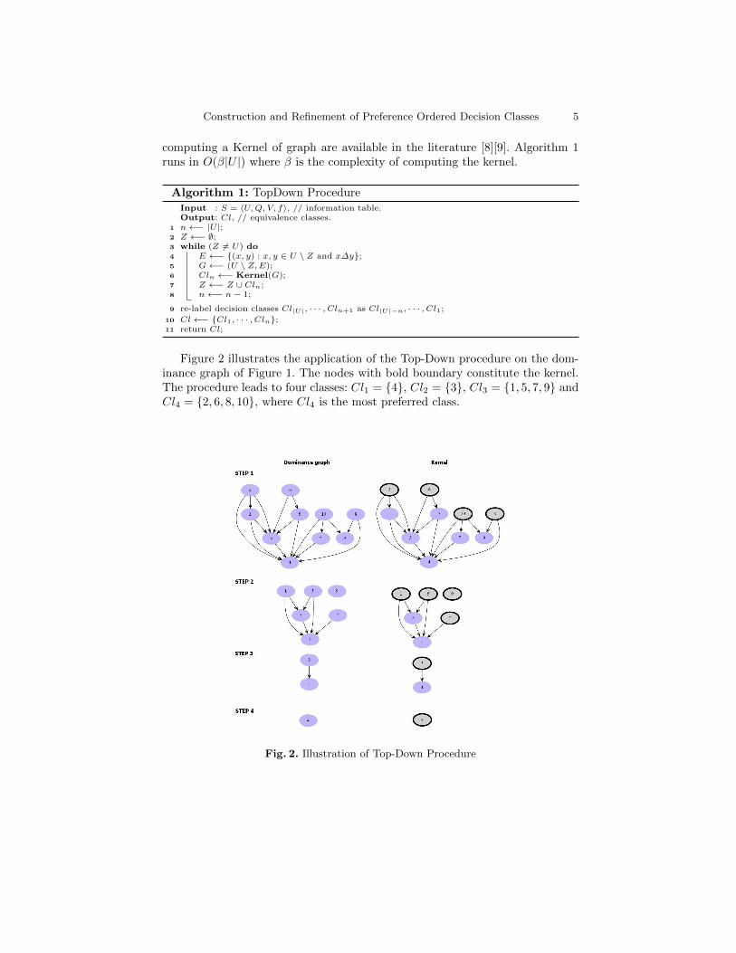
Figure 2 illustrates the application of the Top-Down procedure on the dom-inance graph of Figure 1. The nodes with bold boundary constitute the kernel.The procedure leads to four classes: Cl1 = {4}, Cl2 = {3}, Cl3 = {1, 5, 7, 9} andCl4 = {2, 6, 8, 10}, where Cl4 is the most preferred class.

Fig. 2. Illustration of Top-Down Procedure

6 H.N. Dau et al.

3.2 Bottom-Up Procedure

The set of decision classes can also be induced by examining the directed graphG = (U,E) from bottom to up. First, we identify a minimal subset M ⊆ U suchthat: (i) any decision object that is not in M dominates at least one decisionobject from M ; and (ii) the objects in set M are incomparable. We call set Mthe anti-kernel of graph G. The elements of M are assigned to the less preferreddecision class Cl1. Then, the same procedure is used to identify the anti-kernelM ′ of the sub-graph G′ = (U \ M,E′) and the elements of set M ′ are thenassigned to the second less preferred decision class Cl2. The same procedure isrepeated until all the objects are assigned. This idea is formalized in Algorithm 2.The procedure AntiKernel in this algorithm permits to compute the anti-kernelof the graph given as parameter. The procedures for identifying the AntiKernelof a graph can be obtained by adapting those used to compute graph Kernels[8][9]. Algorithm 2 runs in O(γ|U |) where γ is the complexity of computing theanti-kernel.

Algorithm 2: BottomUp ProcedureInput : S = 〈U,Q, V, f〉, // information table.Output: Cl, // equivalence classes.

1 n←− 1;2 Z ←− ∅;3 while (Z 6= U) do4 E ←− {(x, y) : x, y ∈ U \ Z and y∆x};5 G←− (U \ Z,E);6 Cln ←− AntiKernel(G);7 Z ←− Z ∪ Cln;8 n←− n+ 1;

9 Cl←− {Cl1, · · · , Cln−1};10 return Cl;

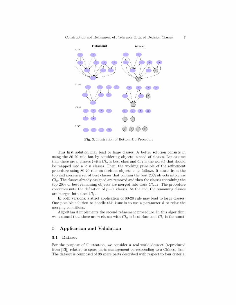
Figure 3 illustrates the application of the Bottom-Up procedure on the dom-inance graph of Figure 1. The nodes with double circle boundary constitute theanti-kernel. The procedure leads to four classes: Cl1 = {4, 9}, Cl2 = {3, 7},Cl3 = {1, 5} and Cl4 = {2, 6, 8, 10}, where Cl4 is the most preferred class.

4 Refinement of Decision Classes

The number of decision classes may be very high. Hence, there is a need to reducethe number of these classes to obtain a manageable set of decision classes. Twosimple refinement procedures that rely on the 80-20 rule are proposed in thispaper. The 80-20 principle (also known as Pareto principle) relies on the factthat, for many events, roughly 80% of the effects come from 20% of the causes.

Let assume that there are n classes (with Cln is best class and Cl1 is theworst) that should be mapped into p < n classes. The first refinement procedurestarts from the top and merge the 20% best classes into class Clp. The classesalready assigned are removed and then the 20% of best classes of the remainingones are merged to class Clp−1. The algorithm continues until the definition ofp− 1 classes. At the end, the remaining classes are merged into class Cl1.

Construction and Refinement of Preference Ordered Decision Classes 7

Fig. 3. Illustration of Bottom-Up Procedure

This first solution may lead to large classes. A better solution consists inusing the 80-20 rule but by considering objects instead of classes. Let assumethat there are n classes (with Cln is best class and Cl1 is the worst) that shouldbe mapped into p < n classes. Then, the working principle of the refinementprocedure using 80-20 rule on decision objects is as follows. It starts from thetop and merges a set of best classes that contain the best 20% objects into classClp. The classes already assigned are removed and then the classes containing thetop 20% of best remaining objects are merged into class Clp−1. The procedurecontinues until the definition of p− 1 classes. At the end, the remaining classesare merged into class Cl1.

In both versions, a strict application of 80-20 rule may lead to large classes.One possible solution to handle this issue is to use a parameter ϑ to relax themerging conditions.

Algorithm 3 implements the second refinement procedure. In this algorithm,we assumed that there are n classes with Cln is best class and Cl1 is the worst.

5 Application and Validation

5.1 Dataset

For the purpose of illustration, we consider a real-world dataset (reproducedfrom [13]) relative to spare parts management corresponding to a Chinese firm.The dataset is composed of 98 spare parts described with respect to four criteria,

8 H.N. Dau et al.

Algorithm 3: Refinement Using 80-20 Rule on Decision Objects

Input : L = {Cl1, · · · , Cln}, // initial classes.β, // integer.

Output: O = {K1, · · · ,Kp}, // refined classes.1 i←− n;2 while (i ≥ 2) do3 Ki ←− top classes in L containing the top 20%± ϑ best objects;4 L←− L \Ki;5 i←− i− 1;

6 K1 ←− L;7 O ←− {K1, · · · ,Kp};8 return O;

namely A1 (Criticality), A2 (Annual Dollar Usage), A3 (Average Unit Cost), andA4 (Lead Time) (see Table 3). The criteria A2 and A3 are continuous while A1

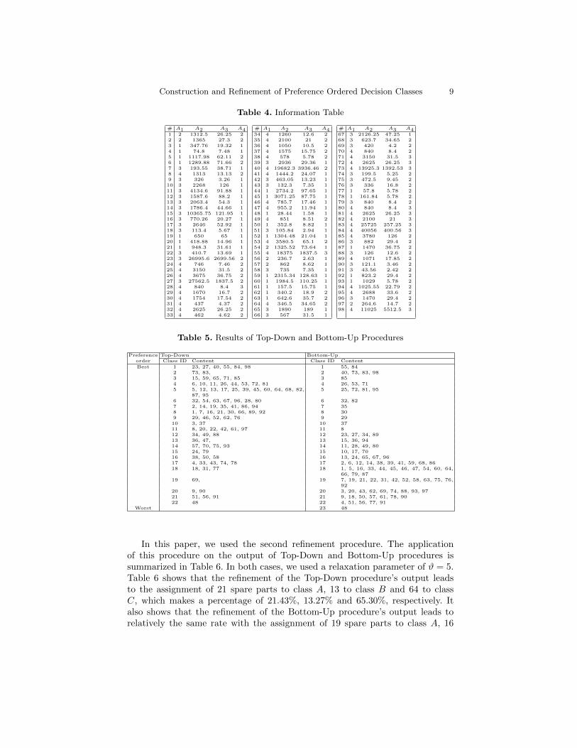
and A4 criteria are ordinal. The criterion A1 can take one of four values 1, 2, 3and 4 where 1 corresponds to the lowest criticality and 4 corresponds to highestcritically. The possible values for A4 are 1, 2 and 3 where 1 means a low leadtime and 3 means a high lead time. All the criteria are benefit-type (i.e. thehigher their values, the more important spare part is). The evaluation of thespare parts with respect to criteria is given in Table 4.

Table 3. Characteristics of Considered Criteria

Code Name Description Preference Data typeA1 Criticality It represents the influence of spare parts

running out on the availability of equip-ment.

Gain Ordinal

A2 Annual Dollar Usage It is calculated by spare part cost multi-ply demand volume.

Gain Continuous

A3 Average Unit Cost It refers to spare part cost. Gain ContinuousA4 Lead Time It refers to the time between the place-

ment of an order and delivery of a newspare part from the firm’s supplier.

Gain Ordinal

5.2 Application and Results

We applied the Top-Down and Bottom-Up procedures using the dataset givenin Table 4. The results of these procedures are given in Table 5. As shown inthis table, the use of the Top-down procedure leads to 22 classes with class #1is the most preferred and class #22 is the worst while the application of theBottom-Up procedure leads to 23 classes with class #23 is most preferred andclass #1 is the worst. As shown in Table 5, both the Top-Down and Bottom-Up procedures lead to a high number of classes and should be mapped into areduced set of classes. Let assume that the obtained decision classes should bemapped into p = 3 ordered decision classes, labelled A, B and C, respectively.

Construction and Refinement of Preference Ordered Decision Classes 9

Table 4. Information Table

# A1 A2 A3 A41 2 1312.5 26.25 22 2 1365 27.3 23 1 347.76 19.32 14 1 74.8 7.48 15 1 1117.98 62.11 26 1 1289.88 71.66 27 3 193.55 38.71 18 4 1313 13.13 29 3 326 3.26 110 3 2268 126 111 3 4134.6 91.88 112 3 1587.6 88.2 113 3 2063.4 54.3 114 3 1786.4 44.66 115 3 10365.75 121.95 116 3 770.26 20.27 117 3 2646 52.92 118 3 113.4 5.67 119 1 650 65 120 1 418.88 14.96 121 1 948.3 31.61 122 3 410.7 13.69 123 3 26995.6 2699.56 224 4 746 7.46 225 4 3150 31.5 226 4 3675 36.75 227 3 27562.5 1837.5 228 4 840 8.4 329 4 1670 16.7 230 4 1754 17.54 231 4 437 4.37 232 4 2625 26.25 233 4 462 4.62 2

# A1 A2 A3 A434 4 1260 12.6 235 4 2100 21 236 4 1050 10.5 237 4 1575 15.75 238 4 578 5.78 239 3 2936 29.36 140 4 19682.3 3936.46 241 4 1444.2 24.07 142 3 463.05 13.23 143 3 132.3 7.35 144 1 2734.2 97.65 145 1 3071.25 87.75 146 4 785.7 17.46 147 4 955.2 11.94 148 1 28.44 1.58 149 4 851 8.51 250 1 352.8 8.82 151 3 105.84 2.94 152 1 1304.48 21.04 153 4 3580.5 65.1 254 2 1325.52 73.64 155 4 18375 1837.5 356 2 236.7 2.63 157 2 862 8.62 158 3 735 7.35 159 1 2315.34 128.63 160 1 1984.5 110.25 161 1 157.5 15.75 162 1 340.2 18.9 263 1 642.6 35.7 264 4 346.5 34.65 265 3 1890 189 166 3 567 31.5 1

# A1 A2 A3 A467 3 2126.25 47.25 168 3 623.7 34.65 269 3 420 4.2 270 4 840 8.4 271 4 3150 31.5 372 4 2625 26.25 373 4 13925.3 1392.53 374 3 199.5 5.25 275 3 472.5 9.45 276 3 336 16.8 277 1 57.8 5.78 278 1 161.84 5.78 279 3 840 8.4 280 4 840 8.4 381 4 2625 26.25 382 4 2100 21 383 4 25725 257.25 384 4 40056 400.56 385 4 3780 126 286 3 882 29.4 287 1 1470 36.75 288 3 126 12.6 289 4 1071 17.85 290 3 121.1 3.46 291 3 43.56 2.42 292 1 823.2 29.4 293 1 1029 5.78 294 4 1025.55 22.79 295 4 2688 33.6 296 3 1470 29.4 297 2 264.6 14.7 298 4 11025 5512.5 3

Table 5. Results of Top-Down and Bottom-Up Procedures

Preference Top-Down Bottom-Uporder Class ID Content Class ID Content

Best 1 23, 27, 40, 55, 84, 98 1 55, 842 73, 83, 2 40, 73, 83, 983 15, 59, 65, 71, 85 3 854 6, 10, 11, 26, 44, 53, 72, 81 4 26, 53, 715 5, 12, 13, 17, 25, 39, 45, 60, 64, 68, 82,

87, 955 25, 72, 81, 95

6 32, 54, 63, 67, 96, 28, 80 6 32, 827 2, 14, 19, 35, 41, 86, 94 7 358 1, 7, 16, 21, 30, 66, 89, 92 8 309 29, 46, 52, 62, 76 9 2910 3, 37 10 3711 8, 20, 22, 42, 61, 97 11 812 34, 49, 88 12 23, 27, 34, 8913 36, 47, 13 15, 36, 9414 57, 70, 75, 93 14 11, 28, 49, 8015 24, 79 15 10, 17, 7016 38, 50, 58 16 13, 24, 65, 67, 9617 4, 33, 43, 74, 78 17 2, 6, 12, 14, 38, 39, 41, 59, 68, 8618 18, 31, 77 18 1, 5, 16, 33, 44, 45, 46, 47, 54, 60, 64,

66, 79, 8719 69, 19 7, 19, 21, 22, 31, 42, 52, 58, 63, 75, 76,

9220 9, 90 20 3, 20, 43, 62, 69, 74, 88, 93, 9721 51, 56, 91 21 9, 18, 50, 57, 61, 78, 9022 48 22 4, 51, 56, 77, 91

Worst 23 48

In this paper, we used the second refinement procedure. The applicationof this procedure on the output of Top-Down and Bottom-Up procedures issummarized in Table 6. In both cases, we used a relaxation parameter of ϑ = 5.Table 6 shows that the refinement of the Top-Down procedure’s output leadsto the assignment of 21 spare parts to class A, 13 to class B and 64 to classC, which makes a percentage of 21.43%, 13.27% and 65.30%, respectively. Italso shows that the refinement of the Bottom-Up procedure’s output leads torelatively the same rate with the assignment of 19 spare parts to class A, 16

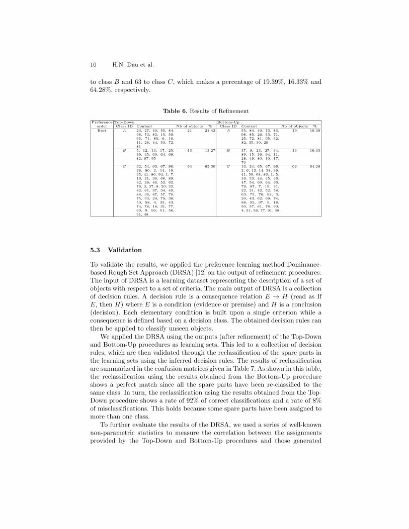
10 H.N. Dau et al.

to class B and 63 to class C, which makes a percentage of 19.39%, 16.33% and64.28%, respectively.

Table 6. Results of Refinement

Preference Top-Down Bottom-Uporder Class ID Content Nb of objects % Class ID Content Nb of objects %

Best A 23, 27, 40, 55, 84,98, 73, 83, 15, 59,65, 71, 85, 6, 10,11, 26, 44, 53, 72,81

21 21.43 A 55, 84, 40, 73, 83,98, 85, 26, 53, 71,25, 72, 81, 95, 32,82, 35, 30, 29

19 19.39

B 5, 12, 13, 17, 25,39, 45, 60, 64, 68,82, 87, 95

13 13.27 B 37, 8, 23, 27, 34,89, 15, 36, 94, 11,28, 49, 80, 10, 17,70

16 16.33

C 32, 54, 63, 67, 96,28, 80, 2, 14, 19,35, 41, 86, 94, 1, 7,16, 21, 30, 66, 89,92, 29, 46, 52, 62,76, 3, 37, 8, 20, 22,42, 61, 97, 34, 49,88, 36, 47, 57, 70,75, 93, 24, 79, 38,50, 58, 4, 33, 43,74, 78, 18, 31, 77,69, 9, 90, 51, 56,91, 48

64 65.30 C 13, 24, 65, 67, 96,2, 6, 12, 14, 38, 39,41, 59, 68, 86, 1, 5,16, 33, 44, 45, 46,47, 54, 60, 64, 66,79, 87, 7, 19, 21,22, 31, 42, 52, 58,63, 75, 76, 92, 3,20, 43, 62, 69, 74,88, 93, 97, 9, 18,50, 57, 61, 78, 90,4, 51, 56, 77, 91, 48

63 64.28

5.3 Validation

To validate the results, we applied the preference learning method Dominance-based Rough Set Approach (DRSA) [12] on the output of refinement procedures.The input of DRSA is a learning dataset representing the description of a set ofobjects with respect to a set of criteria. The main output of DRSA is a collectionof decision rules. A decision rule is a consequence relation E → H (read as IfE, then H) where E is a condition (evidence or premise) and H is a conclusion(decision). Each elementary condition is built upon a single criterion while aconsequence is defined based on a decision class. The obtained decision rules canthen be applied to classify unseen objects.

We applied the DRSA using the outputs (after refinement) of the Top-Downand Bottom-Up procedures as learning sets. This led to a collection of decisionrules, which are then validated through the reclassification of the spare parts inthe learning sets using the inferred decision rules. The results of reclassificationare summarized in the confusion matrices given in Table 7. As shown in this table,the reclassification using the results obtained from the Bottom-Up procedureshows a perfect match since all the spare parts have been re-classified to thesame class. In turn, the reclassification using the results obtained from the Top-Down procedure shows a rate of 92% of correct classifications and a rate of 8%of misclassifications. This holds because some spare parts have been assigned tomore than one class.

To further evaluate the results of the DRSA, we used a series of well-knownnon-parametric statistics to measure the correlation between the assignmentsprovided by the Top-Down and Bottom-Up procedures and those generated

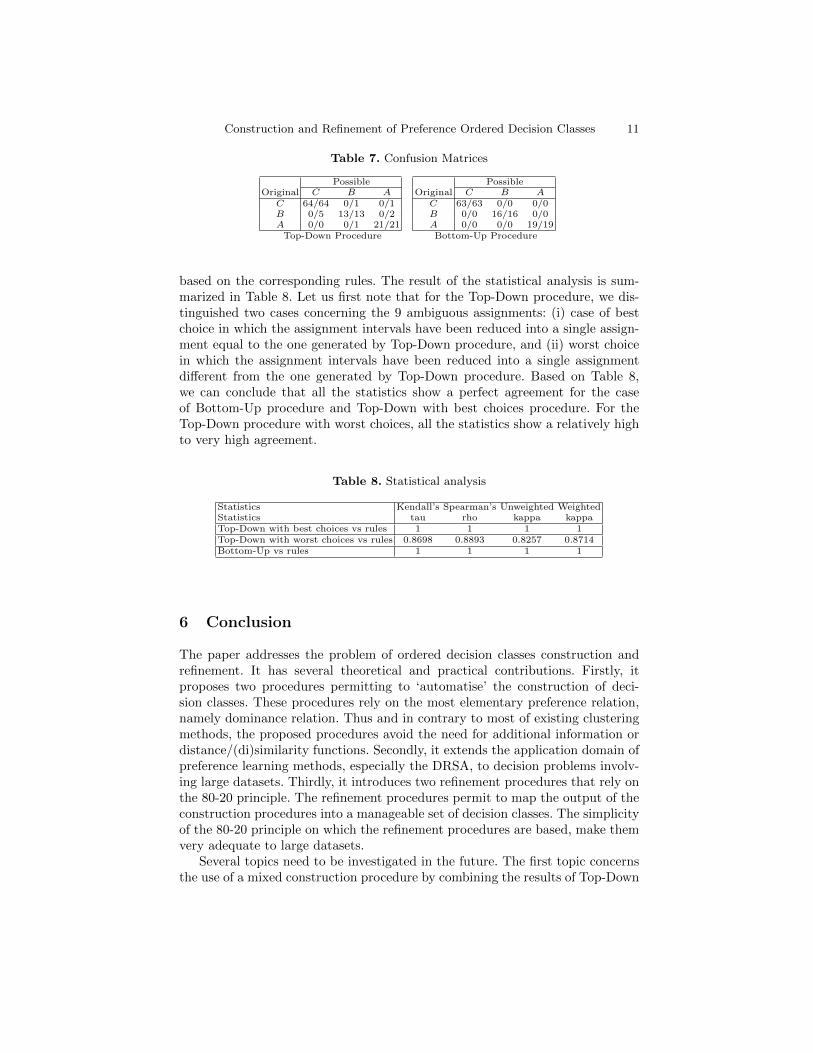
Construction and Refinement of Preference Ordered Decision Classes 11

Table 7. Confusion Matrices

PossibleOriginal C B A

C 64/64 0/1 0/1B 0/5 13/13 0/2A 0/0 0/1 21/21

PossibleOriginal C B A

C 63/63 0/0 0/0B 0/0 16/16 0/0A 0/0 0/0 19/19

Top-Down Procedure Bottom-Up Procedure

based on the corresponding rules. The result of the statistical analysis is sum-marized in Table 8. Let us first note that for the Top-Down procedure, we dis-tinguished two cases concerning the 9 ambiguous assignments: (i) case of bestchoice in which the assignment intervals have been reduced into a single assign-ment equal to the one generated by Top-Down procedure, and (ii) worst choicein which the assignment intervals have been reduced into a single assignmentdifferent from the one generated by Top-Down procedure. Based on Table 8,we can conclude that all the statistics show a perfect agreement for the caseof Bottom-Up procedure and Top-Down with best choices procedure. For theTop-Down procedure with worst choices, all the statistics show a relatively highto very high agreement.

Table 8. Statistical analysis

Statistics Kendall’s Spearman’s Unweighted WeightedStatistics tau rho kappa kappaTop-Down with best choices vs rules 1 1 1 1Top-Down with worst choices vs rules 0.8698 0.8893 0.8257 0.8714Bottom-Up vs rules 1 1 1 1

6 Conclusion

The paper addresses the problem of ordered decision classes construction andrefinement. It has several theoretical and practical contributions. Firstly, itproposes two procedures permitting to ‘automatise’ the construction of deci-sion classes. These procedures rely on the most elementary preference relation,namely dominance relation. Thus and in contrary to most of existing clusteringmethods, the proposed procedures avoid the need for additional information ordistance/(di)similarity functions. Secondly, it extends the application domain ofpreference learning methods, especially the DRSA, to decision problems involv-ing large datasets. Thirdly, it introduces two refinement procedures that rely onthe 80-20 principle. The refinement procedures permit to map the output of theconstruction procedures into a manageable set of decision classes. The simplicityof the 80-20 principle on which the refinement procedures are based, make themvery adequate to large datasets.

Several topics need to be investigated in the future. The first topic concernsthe use of a mixed construction procedure by combining the results of Top-Down

12 H.N. Dau et al.

and Bottom-Up procedures. The second topic is related to the application andperformance evaluation of the procedures with very large data sets. The lasttopic concerns the use of other refinement techniques.

References

1. Albatineh, A., M.Niewiadomska-Bugaj: MCS: A method for finding the numberof clusters. Journal of Classification 28(2) (2011) 184–209

2. Baroudi, R., Bahloul, S.: A multicriteria clustering approach based on similarityindices and clustering ensemble techniques. International Journal of InformationTechnology and Decision Making 13(04) (2014) 811–837

3. Bregar, A., Gyorkos, J., Juric, M.: Interactive aggregation/disaggregation di-chotomic sorting procedure for group decision analysis based on the thresholdmodel. Informatica 19(2) (2008) 161–190

4. de la Paz-Marın, M., Gutierrez, P., Hervas-Martınez, C.: Classification of countries’progress toward a knowledge economy based on machine learning classificationtechniques. Expert Systems with Applications 42(1) (2015) 562–572

5. De Smet, Y.: P2CLUST: An extension of PROMETHEE II for multicriteria or-dered clustering. In: Industrial Engineering and Engineering Management (IEEM),2013 IEEE International Conference on. (Dec 2013) 848–851

6. De Smet, Y.: An extension of PROMETHEE to divisive hierarchical multicriteriaclustering. In: Industrial Engineering and Engineering Management (IEEM), 2014IEEE International Conference on. (Dec 2014) 555–558

7. De Smet, Y., Nemery, P., Selvaraj, R.: An exact algorithm for the multicriteriaordered clustering problem. Omega 40(6) (2012) 861–869

8. Emmert-Streib, F., Dehmer, M., Shi, Y.: Fifty years of graph matching, networkalignment and network comparison. Information Sciences 346-347 (2016) 180–197

9. Ghosh, S., Das, N., calves, T.G., Quaresma, P., Kundu, M.: The journey of graphkernels through two decades. Computer Science Review 27 (2018) 88–111

10. Gilboa, I., Schmeidler, D.: Case-based knowledge and induction. IEEE Transac-tions on Systems, Man, and Cybernetics: Part A 30(2) (2000) 85–95

11. Gionis, A., Mannila, H., Tsaparas, P.: Clustering aggregation. ACM Transactionson Knowledge Discovery from Data 1(1) (2007) Article 4.

12. Greco, S., Matarazzo, B., S lowinski, R.: Rough sets theory for multicriteria decisionanalysis. European Journal of Operational Research 129(1) (2001) 1–47

13. Hu, Q., Chakhar, S., Siraj, S., Labib, A.: Spare parts classification in industrialmanufacturing using the dominance-based rough set approach. European Journalof Operational Research 262(3) (2017) 1136–1163

14. Rocha, C., Dias, L.: MPOC: an agglomerative algorithm for multicriteria partiallyordered clustering. 4OR 11(3) (2013) 253–273