Parallel Iterative Refinement in Polynomial Eigenvalue

Problems∗

Carmen Campos Jose E. Roman

March 4, 2016

Abstract

Methods for the polynomial eigenvalue problem sometimes need to be followed by an it-erative refinement process to improve the accuracy of the computed solutions. This can beaccomplished by means of a Newton iteration tailored to matrix polynomials. The computa-tional cost of this step is usually higher than the cost of computing the initial approximations,due to the need of solving multiple linear systems of equations with a bordered coefficient ma-trix. An effective parallelization is thus important, and we propose different approaches for themessage-passing scenario. Some schemes use a subcommunicator strategy in order to improvethe scalability whenever direct linear solvers are used. We show performance results for thevarious alternatives implemented in the context of SLEPc, the Scalable Library for EigenvalueProblem Computations.

1 Introduction

We are interested in the accurate computation of a few eigenpairs (x, λ) of the polynomial eigenvalueproblem, defined as

P (λ)x = 0, x 6= 0, (1)

where λ ∈ C is the eigenvalue, x ∈ Cn is the eigenvector, and P (·) is an n × n matrix polynomialof degree d. This problem appears in many practical applications, for instance when discretizing asecond (or higher) order partial differential equation, and also as an intermediate tool for solvinggeneral nonlinear eigenproblems, e.g., via interpolation. Many of the examples described in theNLEVP collection [5] are polynomial eigenproblems. Throughout the paper we will assume thatthe matrix polynomial is regular, that is, detP (λ) is not identically zero.

Instead of the usual monomial form, in this paper we express the matrix polynomial in termsof a more general polynomial basis,

P (λ) = Φ0(λ)A0 + · · ·+ Φd(λ)Ad, (2)

∗This work was partially supported by the Spanish Ministry of Economy and Competitiveness under grantTIN2013-41049-P. Carmen Campos was supported by the Spanish Ministry of Education, Culture and Sport throughan FPU grant with reference AP2012-0608. The computational experiments of section 5 were carried out on thesupercomputer Tirant at Universitat de Valencia.

1

where {Φj(λ)}∞j=0 is a sequence of real polynomials with Φj(λ) of degree j satisfying a 3-termrecurrence

λΦj(λ) = αj Φj+1(λ) + βj Φj(λ) + γj Φj−1(λ), for j = 1, 2, . . . (3)

where Φ−1 ≡ 0, Φ0 ≡ 1, and for j = 0, 1, . . . , αj , βj and γj are real, αj > 0 and αj =cj

cj+1, with cj

being the leading coefficient of Φj(λ) [2, 7]. These include Chebyshev polynomials among others.This approach may be more reliable numerically than the monomial basis in the case of high degreepolynomials, especially when the eigenvalues are located on (or close to) an interval of the real axis.

We focus on the particular case of large-scale problems, where the polynomial coefficients Ai aresparse matrices, and only a few eigensolutions are required. The most common approach for thisscenario is to apply a projection method on a certain linearization of the matrix polynomial: first,build matrices L0 and L1 of order dn such that the eigenvalues of the pencil L0−λL1 coincide withthose of (1), then get approximate solutions by projecting this linear problem onto a subspace built,e.g., with a Krylov iteration. Krylov methods for the linearized eigenproblem have been addressedin, e.g., [18]. It is possible to formulate variants of well-known Krylov methods that are able toexploit the structure of L0 and L1 from the linearization, resulting in very efficient algorithms interms of memory as well as computational cost [7].

For problems of large dimension, parallel computing is required. We have implemented solversbased on Krylov iterations on the linearization, as sketched above, where the problem matricesAi as well as the associated vectors are distributed across available processes and message-passing(with MPI) is employed to coordinate the required computations. Our solvers, that are describedin detail in [7], have been implemented in SLEPc, the Scalable Library for Eigenvalue ProblemComputations [10, 15], which is an extension of PETSc (Portable, Extensible Toolkit for ScientificComputation [3]). In the context of this kind of computations, it is often necessary to perform linearsystem solves, and this can be done with iterative methods provided by PETSc or, alternatively,with direct methods from a third-party solver such as MUMPS [1].

The overall solution process based on linearizing the polynomial is not guaranteed to be back-ward stable, even if a backward stable method is employed for the linear eigenproblem [12]. Hence,robust polynomial eigensolvers such as those included in SLEPc must provide an effective way ofimproving the accuracy of the computed solution. This is done with iterative refinement, where thecomputed solution is fed as the starting guess for one (or more) Newton iteration. We remark thatscaling the coefficient matrices can sometimes improve the conditioning of the linearized eigenprob-lem, hence improving accuracy, but it is not effective in some problems with degree larger than 2.In our codes, users can choose to perform scaling as described in [4] (see implementation details in[7]), but we do not consider it in this paper since operation of the refinement algorithm is the sameregardless of whether the matrices have been scaled or not.

Iterative refinement for the linear eigenvalue problem has been addressed by Tisseur [17]. Forthe polynomial eigenproblem, iterative refinement can be formulated in terms of a single eigenpair(x, λ) or, more generally, in terms of invariant pairs (X,H). Invariant pairs [14] are a generalizationof invariant subspaces for nonlinear eigenvalue problems, and they will be defined in §2 for matrixpolynomials. Kressner [14] formulates a Newton iteration that operates on invariant pairs, aimingat refining solutions of nonlinear eigenvalue problems. This method was later particularized to thecase of polynomial eigenproblems [6].

In this paper, we provide all the details regarding the implementation of Newton iterativerefinement for polynomial eigenproblems in SLEPc, as a way to complement the description ofthe solvers in [7]. Our implementation is based on [14] and is therefore more general than [6],since we do not restrict ourselves to polynomials expressed in the monomial basis and formulate

2

the methods assuming polynomial bases of the form (3). We focus particularly on the aspects ofparallel computing, since the Newton step can be very costly as it usually involves many linearsystem solves. We propose several alternatives to organize this computation, and analyze how allthese solutions scale when the number of processes increase. For this, it will sometimes be useful toorganize the participating processes in several subcommunicators, especially if direct linear solversare to be used.

The rest of the paper is organized as follows. Section 2 provides the formal definition of invariantpair and summarizes the essentials of Krylov methods available in SLEPc to solve (1). Section 3describes the Newton method for polynomial eigenproblems [6], adapting it to the non-monomialform of the polynomial, (2). Section 4 gives a description of the different variants proposed to solvethe linear systems, together with details of the parallel implementation. Computational results areprovided in §5. Finally, we wrap up with some concluding remarks.

2 Computing invariant pairs

When solving a linear eigenvalue problem, it is known that computing invariant subspaces insteadof several eigenvectors may have better numerical behaviour, e.g., when the matrix of computedeigenvectors has a large condition number. This is also the case when computing a few eigenpairsassociated with a polynomial eigenproblem (1), although in this latter case, as explained in [6, 14],the concept of invariant subspace should be substituted with the concept of invariant pair.

Definition 1. Given (X,H) ∈ Cn×k ×Ck×k, it is said to be an invariant pair for a regular matrixpolynomial defined as in (2) if

P(X,H) := A0X Φ0(H) +A1X Φ1(H) + · · ·+AdX Φd(H) = 0, (4)

where Φi(H) stands for the matrix function defined by the polynomial Φi, see [11].

For linear eigenproblems, eigenvalues of the H matrix from an invariant pair, (X,H), are alsoeigenvalues of the linear eigenproblem provided that X has full column rank. For nonlinear eigen-problems, this assumption has to be replaced by minimality [14, lemma 4]. In the case of matrixpolynomials expressed in the form (2), we will use a similar concept to guarantee that eigenvaluesof H are indeed eigenvalues for the eigenproblem (1).

2.1 Linearization

We focus on methods that approximate the solution of a polynomial eigenproblem of dimensionn and degree d via linearization. In these methods the involved vectors have length dn. We willconsider that vectors v ∈ Cdn and tall-skinny matrices V ∈ Cdn×k are divided in d blocks of n rows,

v =

v0

...vd−1

, V =

V 0

...V d−1

, (5)

where vi ∈ Cn and V i ∈ Cn×k for i = 0, . . . , d − 1. Throughout the text, we will use superindicesto denote each of the blocks of the split form (5).

3

We will suppose that polynomial eigensolvers used for (1) are based on the following linearization(details can be found in [7]):

L(λ) = L0 − λL1, (6)

L0 =

β0I α0Iγ1I β1I α1I

. . .. . .

. . .

. . .. . .

. . .

γd−2I βd−2I αd−2I

A0 A1 A2 · · · Ad−3 Ad−2 Ad−1

, L1 =

I

. . .

IcdAd

,

with Aj = −cd−1Aj (j = 0, . . . , d− 3), Ad−2 = −cd−1Ad−2 + cdγd−1Ad and Ad−1 = −cd−1Ad−1 +cdβd−1Ad. This is a strong linearization and therefore L(λ)z = 0 and (1) share the same eigen-values with the same algebraic and geometric multiplicities (details in [2] and references therein).Furthermore, the eigenvector z has the structure

z =

x

Φ1(λ)x...

Φd−1(λ)x

, (7)

with x being the corresponding eigenvector of the polynomial eigenproblem (1). Proposition 1shows that it is possible to extend this expression to invariant pairs.

Proposition 1. Let (Z,H) be an invariant pair of the linearized problem (6) in which Z has fullrank, then the following holds:

1. Z = Vd(Z0, H), where Vm(X,H) is defined for m ∈ N, X ∈ Cn×k and H ∈ Ck×k as

Vm(X,H) :=

X

X Φ1(H)...

X Φm−1(H)

. (8)

2. (Z0, H) is an invariant pair of the polynomial eigenproblem (1) satisfying that each eigenvalueof H is also an eigenvalue of (1).

Proof. Since (Z,H) is an invariant pair for the linearization, we have that L0Z −L1ZH = 0 for L0

and L1 given in (6). By equating the first d− 1 block rows of this equation, we obtain{Z1 = α−1

0 (Z0H − β0Z0),

Zi = α−1i−1(Zi−1H − βi−1Z

i−1 − γi−1Zi−2), i = 2, . . . , d− 1.

(9)

These equations allow us to prove easily by induction that

Zi = Z0 Φi(H), i = 0, 1, . . . , d− 1. (10)

4

To prove the second statement, we equate the last block row of the equation L0Z−L1ZH = 0, andwe obtain that

0 = −cd−1

d−1∑i=0

AiVi + cdγd−1AdV

d−2 + cdβd−1AdVd−1 − cdAdV

d−1H =

= −cd−1

d−1∑i=0

AiV0 Φi(H)− cdAdV

0(Φd−1(H)H − βd−1 Φd−1(H)− γd−1 Φd−2(H)) =

= −cd−1

d−1∑i=0

AiV0 Φi(H)− cdαd−1AdV

0 Φd(H) = −cd−1

d∑i=0

AiV0 Φi(H),

from where we conclude that (V 0, H) is an invariant pair of (1). On the other hand, for an eigenpairof H, (y, λ), we have that (Zy, λ) is an eigenpair of the linearized problem (Z has full rank), so ithas form (7) and we conclude that there exists some x eigenvector of (1) associated with λ.

Proposition 1 states that it is always possible to extract an invariant pair of the polynomialeigenvalue problem (1) from one for the linearized problem, by taking the first block Z0. Otherextraction alternatives that make use of other blocks Zi have been proposed in [6] for polynomialeigenproblems defined in terms of the monomial basis, and their counterparts for non-monomialbases are implemented in SLEPc.

The converse of Proposition 1 is also true:

Proposition 2. Let (X,H) be an invariant pair of the polynomial eigenproblem (1), then Z :=Vd(X,H) is an invariant pair for the linearized problem (6).

Proof. The proof is a simple verification of the equality L0Z = L1ZH. As in Proposition 1, thefirst d−1 row blocks of this equality are checked using the recurrence (3), and the last one usingthe condition of (X,H) satisfying (4).

Remark. As a consequence of Propositions 1 and 2 we have that, for an invariant pair of (1), (X,H),such that Vd(X,H) has full column rank, every eigenvalue of H is also an eigenvalue of (1). In thiscase, taking as reference the definition given in [6], we say that (X,H) is a minimal invariant pairof (1).

A property needed to ensure convergence in the Newton process described in §3 is the concept ofsimple invariant pair. A minimal invariant pair of (1) is said to be simple if the algebraic multiplicityof each eigenvalue of H matches the algebraic multiplicity of these same eigenvalues in (1) (that is,the multiplicity as a root of the characteristic polynomial detP (λ)). Since the linearization (6) is astrong linearization for (1), if the computed invariant pair for the linearized eigenproblem is simple,then the corresponding invariant pair for the polynomial eigenproblem (1) will also be simple.

2.2 Krylov methods for the linearized polynomial eigenproblem

The Newton process described in §3 starts from an approximate simple invariant pair for thepolynomial eigenproblem, and it improves its accuracy iteratively. In this section, we briefly reviewthe methods we use to compute the initial approximate invariant pair. These methods are describedin [7], and all of them are based on solving the linearized problem (6) using the Krylov-Schur methodand extracting a minimal invariant pair for (1) from the one computed for (6).

5

Krylov-Schur [16] is an implicitly restarted variant of the Arnoldi method. Starting from aninitial vector v ∈ Cn, Arnoldi generates an orthogonal basis {v1, . . . , vk+1} of the Krylov subspaceKk+1(M,v) := span{v,Mv, . . . ,Mkv}, and the projected matrix Hk = V ∗k MVk verifying,

MVk = VkHk + βkvk+1e∗k, (11)

where βk ∈ R, M = L−11 L0 (or M = (L0 − σL1)−1L1 if a shift-and-invert transformation is used),

Vk := [v1, . . . , vk], and e∗k = [0, 0, . . . , 0, 1].When, for a particular value of k, the norm of the residual MVk − VkHk = βkvk+1e

∗k is small

enough, the Krylov-Schur process is considered to be converged and then (Vk, Hk) is an approximateminimal invariant pair for (6) in which the columns of Vk are orthonormal.

The main two variants of the SLEPc polynomial solvers described in [7] differ in the way that thevj vectors are stored. These variants are, on one hand, Plain Arnoldi that stores full-sized Arnoldivectors of dimension dn, and, on the other hand, the TOAR variant that generates an orthonormalset, Uk+d ∈ Cn×(k+d) and matrices {Gi

k+1}d−1i=0 ⊂ C(k+d)×(k+1), from which it reconstructs each

block of the Krylov basis Vk+1 as

V ik+1 = Uk+dG

ik+1, i = 0, . . . , d− 1. (12)

In a more compact form, the Krylov vectors are expressed as

Vk+1 = (Id ⊗ Uk+d)Gk+1. (13)

We are interested in showing this notation here because it will be referenced later. Other details ofthe methods can be found in [7].

3 Newton refinement for invariant pairs

In this section, we explain in detail how the iterative refinement of invariant pairs is carried out inSLEPc’s Krylov-based polynomial eigensolvers. We use the Newton iteration for nonlinear eigen-problems described in [14] assuming that the functions fi defining the nonlinear eigenproblem(f0(λ)A0 + · · · + fd(λ)Ad)x = 0 are the polynomials Φi that define the polynomial eigenproblem(1). When it is possible, we simplify some of the associated computations giving expressions similarto those in [6].

Computing a minimal invariant pair of (1) is equivalent to obtaining (X,H) ∈ Cn×k × Ck×k

such that

P(X,H) = 0, and (14a)

V(X,H) := W ∗Vd(X,H)− Ik = 0, (14b)

for some matrix W ∈ Cdn×k with full column rank, and P defined in (4).Applying results in Kressner [14] we obtain that once an approximation (X, H) of a simple

invariant pair (X,H) of (1) has been computed, it can be used as the starting guess for the Newtonmethod applied to the system of nonlinear equations (14), obtaining in this way a refined solution of(1) closer to (X,H). Provided that the initial approximation (X, H) is sufficiently close to (X,H),this method generates a sequence of iterates, {(Xi, Hi)}i∈N that converges quadratically to (X,H).These iterates are given by

(Xi+1, Hi+1) = (Xi, Hi)− (L(Xi, Hi))−1(P(Xi, Hi),V(Xi, Hi)), (15)

6

where L(X,H) := (DP(X,H),DV(X,H)) being DP(X,H) and DV(X,H) the Frechet derivatives,in (X,H), of P and V, respectively. The (local) quadratic convergence of the Newton method isa consequence of [14, Theorem 10] which proves that the linear operator L(X,H) is invertible forsimple invariant pairs.

Algorithm 1 Newton method for refining invariant pairs

Input: Initial pair (X0, H0) ∈ Cn×k × Ck×k such that Vd(X0, H0)∗Vd(X0, H0) = IkOutput: Approximate solution (Xi+1, Hi+1) to (14)

1: W ← Vd(X0, H0)2: for i = 0, 1, . . . ,maxit do3: Compute residual R← P(Xi, Hi)4: Compute (∆X,∆H) such that L(Xi, Hi)(∆X,∆H) = (R, 0)5: Xi+1 ← Xi −∆X, Hi+1 ← Hi −∆H6: Compute compact QR decomposition Vd(Xi+1, Hi+1) = WT7: Xi+1 ← Xi+1T

−1, Hi+1 ← THi+1T−1

8: Check convergence, exit if satisfied9: end for

Algorithm 1 shows the procedure described in [14] to iteratively compute an invariant pair of(1), starting from an approximate simple invariant pair. This algorithm works with orthonormalVd(Xi, Hi) and takes W := Vd(Xi, Hi) so that V(Xi, Hi) = 0 at each iteration. For this, it computesa compact QR decomposition of Vd(Xi+1, Hi+1) and updates the approximate solution (Xi+1, Hi+1)accordingly. Note that for doing this it is not necessary to explicitly compute the QR factorizationof Vd(Xi, Hi) of size (dn × k). The matrix T can be computed in a cheaper way if we decomposeXi = UGi being U ∈ Cn×k with orthonormal columns and Gi ∈ Ck×k. In this case we have that

Vd(Xi, Hi) = (Id ⊗ U)Vd(Gi, Hi) for Vd(Gi, Hi) :=

[Gi Φ0(Hi)

...Gi Φd−1(Hi)

]and T can be obtained from the

QR factorization of Vd(Gi, Hi) = UT .The most expensive step in Algorithm 1 (step 4) involves the solution of a system of linear

matrix equations {DP(Xi, Hi)(∆X,∆H) = P(Xi, Hi)

DV(Xi, Hi)(∆X,∆H) = 0.(16)

More explicitly, for P defined in (4), the system to solve at each refinement iteration isP(∆X,Hi) +

d∑j=0

AjXi D Φj(Hi)(∆H) = P(Xi, Hi)

(W 0)∗∆X +

d−1∑j=1

(W j)∗ (∆X Φj(Hi) +Xi D Φj(Hi)(∆H)) = 0,

(17)

where, for j > 0, D Φj(Hi) represents the Frechet derivative of Φj in Hi, which can be obtained

7

recursively from (3) as:

D Φj(Hi)(∆H) =

0, j = 0

α−10 ∆H, j = 1

α−1j−1

(D Φj−1(Hi)(∆H)(Hi − βj−1I) + Φj−1(Hi)∆H−− γj−1 D Φj−2(Hi)(∆H)

), j > 1.

(18)

To solve (17), we use the forward substitution technique described in [14, 6]. It requires matrixHi being triangular, which is always possible by computing the complex Schur form of Hi andupdating Xi properly. In this case, the columns of ∆X and ∆H are successively computed assolutions of k linear systems of dimension n+k, updating the equation right-hand side at each step.For example, post-multiplying (17) by e1 produces the linear system

P (h11)∆x1 +

d∑j=0

AjXi D Φj(Hi)(∆H)e1 = r1

(W 0)∗∆x1 +

d−1∑j=1

(W j)∗(∆x1 [Φj(Hi)]11 +Xi D Φj(Hi)(∆H)e1

)= f1,

(19)

where ∆x1 and ∆h1 are the first columns of ∆X and ∆H, respectively, h11 and [Φj(Hi)]11 denotethe (1, 1) element of Hi and Φj(Hi) (both of them upper triangular matrices), r1 is the first columnof the residual P(Xi, Hi), and f1 = 0. Defining {D Φj(Hi)}11, for j = 1, . . . , as the triangularmatrix verifying

D Φj(Hi)(C)e1 = {D Φj(Hi)}11 Ce1, ∀C ∈ Ck×k, (20)

results in a linear system from where it is possible to obtain the first columns of ∆X and ∆H,[P (h11)

∑dj=0AjXi {D Φj(Hi)}11∑d−1

j=0 Φj(h11)(W j)∗∑d−1

j=1(W j)∗Xi {D Φj(Hi)}11

] [∆x1

∆h1

]=

[r1

f1

]. (21)

Matrices (20) can be obtained recursively from (18):

{D Φ0(Hi)}11 = 0, {D Φ1(Hi)}11 = α−10 Ik, (22)

{D Φj+1(Hi)}11 = α−1j

((h11 − βj) {D Φj(Hi)}11 + Φj(Hi)− γj {D Φj−1(Hi)}11

), j > 0.

After computing ∆x1 and ∆h1 the right-hand side of (17) is updated before proceeding with thesecond column of ∆Xi and ∆Hi. To compute the successive columns ∆xp and ∆hp, p = 2, . . . , k,we form the corresponding systems analog to (21) by substituting h11 by hpp (also in (22)), andreplacing the right-hand side

[ r1f1

]by the one computed applying consecutive updates according to

rp = P(Xi, Hi)ep −p−1∑q=1

d∑j=0

Aj

(∆xq [Φj(Hi)]qp +Xi [D Φj(Hi)(Zq)]p

) , (23)

fp = −p−1∑q=1

d−1∑j=1

(W j)∗(

∆xq [Φj(Hi)]qp +Xi [D Φj(Hi)(Zq)]p

) ,

8

A

P0

P1

P2

B CT D

Figure 1: Parallel distribution of matrices and vectors.

where [Φj(Hi)]qp denotes the (q, p) element of Φj(Hi), and [D Φj(Hi)(Zq)]p the pth column of

D Φj(Hi)(Zq), being Zq := ∆xqeTq .

In the case of having a simple eigenpair, (xi, λi), of (1), it can also be seen as a simple invariantpair of size k = 1 (clearly Vd(xi, λi) has full column rank). That motivates two refining variantswhen computing a set of q eigenpairs which are included in our solver. The first one is the multiplevariant, which refines the invariant pair of dimension k = q, yielding an invariant pair of the samedimension. On the other hand, the simple variant, which refines each computed simple eigenpairindividually by solving q systems in the form (21) with dimension k = 1. Both options require thesolution of bordered linear systems in which the leading block of order n is a nearly singular matrix.Aiming to minimize the time required by the solution of these systems, in this work we evaluateseveral forms to carry out these solves.

4 Solving the correction equation

In this section, we describe several methods that we have considered for the linear systems arisingin the forward substitution method used to solve the correction equation (17), explained in §3. Wewill also discuss several alternatives relative to their parallel implementation.

The linear systems to be solved, (21), have the form[A BC D

] [x1

x2

]=

[y1

y2

], (24)

where the coefficient matrix is a bordered matrix with blocks A ∈ Cn×n, B ∈ Cn×k, C ∈ Ck×n

and D ∈ Ck×k, with k � n. The leading block A is nearly singular. The parallel distributionof these four submatrices is depicted in Fig. 1. We store D as a sequential matrix (every processowns a copy), and B,C are stored as an array of k parallel vectors. In PETSc, parallel vectorsare distributed by blocks, with each process owning a contiguous range of indices. Regarding thesparse block A, it is stored as a standard PETSc matrix, with every process owning a contiguousrange of rows.

The first alternative, that will be referred to as the explicit matrix approach, corresponds toexplicitly building the whole matrix involved in (21) as a PETSc matrix. This allows using anyof the PETSc linear solvers and preconditioners, including direct solvers, which may be seen as an

9

P0

P1

P2

P0

P1

P2

Figure 2: Illustration of the parallel distribution of the matrix created in the explicit matrix ap-proach before (left) and after (right) applying the symmetric permutation.

advantage. However, this approach presents several drawbacks. On one hand, the coefficient matrixof the linear system to be solved is not very sparse, compared to the sparsity of P (·), since it hasbeen bordered with dense stripes. This affects the fill-in that is produced in the factorization whena direct method is used, and it also has an impact on the performance of parallel matrix-vectormultiplication since processors owning any of the fully populated rows require the whole distributedvector to carry out its computational part in this operation. On the other hand, when the createdmatrix is distributed by blocks of consecutive rows across the involved processes (as mentionedabove) then it will produce load imbalance that can seriously penalize the overall performance.

Aiming to reduce the load imbalance in this first approach, an appropriate symmetric permu-tation of the matrix is distributed among the processes. The permutation is chosen in such a waythat the fully populated rows are evenly distributed across the available processes, by placing themright after the local rows of the leading block A assigned to them. Fig. 2 shows the matrix beforeand after applying the permutation. With this approach, all involved vectors are subject to thesame permutation.

The second option we have evaluated uses the Schur complement of the trailing diagonalblock D in (24),

S := A−BD−1C, (25)

to compute x1 and x2 from

Sx1 = y1 −BD−1y2, (26)

x2 = D−1(y2 − Cx1). (27)

Note that a similar scheme using the Schur complement of the leading diagonal block A in (24) isnot appropriate since it implies linear solves with the nearly singular matrix A.

The matrix S (25) is dense so it should not be explicitly computed. This fact limits the methodsavailable to solve the linear system involved in (26) with the matrix S, which cannot be solved viaa direct solver. Instead, iterative methods such as GMRES or any of the Krylov methods providedby PETSc are adequate for the solves. To build the preconditioner needed for the iterative methodswe have used the approximation to S given by P := A−diag(BD−1C), where the operator diag(M)represents a matrix whose diagonal elements are the same as the matrix M , and have zeros outsidethe diagonal.

A third alternative that enables the use of direct methods when solving (21), is the mixed blockelimination (MBE) method described in [8, 9]. This method solves bordered linear systems in the

10

form (24) making solves with the nearly singular leading block matrix and its transpose. Algorithm2 shows the process followed for this method to solve a linear system with a one-dimensional border,[

A bc d

] [x1

x2

]=

[y1

y2

]. (28)

Algorithm 2 Mixed block elimination (MBE) method

Input: A ∈ Cn×n, b, y1 ∈ Cn×1, c ∈ C1×n and d, y2 ∈ C defining the linear system (28)Output: x ∈ Cn+1 solution of (28) (x = [ x1

x2])

1: Solve AT v = cT

2: δ ← d− vT b3: Solve Aw = b4: ρ← d− cw5: p2 ← (y2 − vT y1)/δ6: g1 ← y1 − bx2

7: g2 ← y2 − dp2

8: Solve Az = g1

9: q2 ← (g2 − cz)/ρ10: x1 ← z − wq2

11: x2 ← p2 + q2

To solve a linear system with a wider border, this method works recursively decreasing thedimension of the border in the linear systems that it generates at each step. For example, to solvea linear system (24) for a border of dimension 2,

n

1

1

n 1 1 A b1c1 d11

b2d12

c2 d21 d22

x1:n

xn+1

xn+2

=

y1:n

yn+1

yn+2

, (29)

using Algorithm 2, the method performs 3 solves with the submatrix[A b1c1 d11

](30)

of dimension n+1, the vectors b :=[

b2d12

], c := [ c2 d21 ] and the right-hand side vector g ∈ Cn+1

computed from y with several updates (steps 1, 3 and 8 of Algorithm 2). These linear systemsare one-dimensional bordered systems as in (28) and they can directly be solved using Algorithm2. Each solve with matrix (30) makes two solves (with A and AT ) that are independent of theright-hand side, thus, the three required solves with matrix (30) and right-hand sides b, c and ghave common computations that can be shared.

In the case of avoiding repeated solves by storing intermediate calculations, the MBE methodrequires 2k+1 solves of dimension n, to solve a bordered linear system of dimension n+k with aborder of dimension k. When using this method in the forward substitution process, the number ofoverall linear solves required by this method could be seen as a strong limitation to the dimensionof the invariant pair to refine. However, in the results of §5 we will see that for moderate values ofk the mixed block elimination shows a good behaviour, compared to the other methods. Moreover,

11

most computations in the MBE method can be done independently of the right-hand side, since2k out of 2k + 1 solves required for this method only involve data from the system matrix. Thisfact represents better opportunities of parallelism, as it alleviates inherent sequentiality of otherapproaches. In particular, the use of subcommunicators will be especially beneficial in this case, asdiscussed below.

The forward substitution process used to solve the correction equation implies solving k linearsystems of size n+ k that, in some cases, need to be solved using a direct method. In this case, theoverall parallel performance can be seriously penalized due to the limited scalability of factorizationssuch as LU, as well as the associated triangular solves. To reduce such limitation we have studied thepossibility of adding a second level of parallelism by splitting the set of MPI processes into severalsubgroups, so that each new subgroup will be responsible for solving some of the linear systemsrequired by the forward substitution procedure. For this, the matrices defining the polynomialeigenproblem are redundantly replicated in each subgroup, and so are the set of distributed vectorsX (the small matrix H is fully stored by each process).

This subcommunicator approach is applicable in both the simple and multiple refinementschemes. In the case of the simple refinement, when refining k individual eigenpairs instead ofan invariant pair of dimension k, the linear systems come from separate refinement processes andthere is complete independence between the resolution of the linear systems, which can be freelydistributed and solved among the subgroups of processes. However, this is not the case for multiplerefinement, due to the forward substitution procedure, where each computed solution updates theright-hand sides of the subsequent linear systems. When forming the right-hand side,

[ rpfp

], of the

pth system to be solved, update (23) is required, involving the previously computed (∆xq,∆hq).This forces the solves to be carried out in a sequential way. Despite that, the building and solvingof these systems also entails several time consuming operations that can be carried out in parallelby the different subgroups, as described in Algorithm 3.

The copy of the parallel matrices and vectors in step 2 of Algorithm 3 represents a data re-distribution requiring communication involving all processes. For example, Fig. 3 shows how amatrix distributed in 5 processes is duplicated redundantly into two subcommunicators with 3 and2 processes, respectively.

In steps 4–11 of Algorithm 3, each subgroup is assigned a different column of ∆X and ∆H to becomputed, calculates the associated bordered matrix and performs a matrix factorization requiredfor using a direct method. The MBE method factorizes the leading submatrix A of (24), whereas theexplicit matrix approach factorizes the full bordered matrix. After that, the dependence betweenthe right-hand sides in the involved linear systems forces a sequential stage for the solves (steps12–17 in Algorithm 3). Despite that, in the case of using MBE, the solution of the bordered systems(24) entails the solution of 2k linear systems with the leading block A which are independent ofthe right-hand side [ y1

y2 ]. Therefore, these solves can be moved to the concurrent phase (step 9 ofAlgorithm 3), and only one right-hand side dependent solve is left in the sequential stage (step 15of Algorithm 3). After a column of ∆X and ∆H has been computed, it is redistributed from thecorresponding subcommunicator to the original global communicator.

The gain when activating this second level of parallelism is limited by the size of the invariantpair to refine (or the number of eigenpairs in the case of simple refinement) but, as will be shownin §5, it relieves the limited scalability of solves based on direct methods.

12

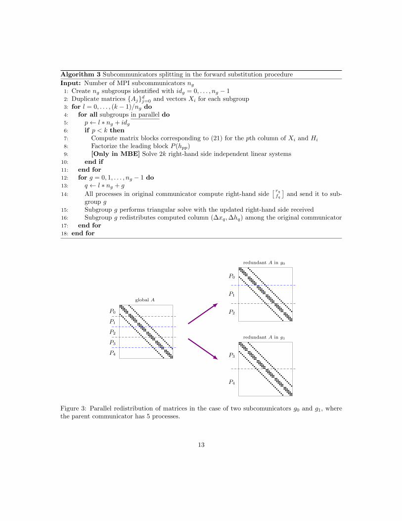
Algorithm 3 Subcommunicators splitting in the forward substitution procedure

Input: Number of MPI subcommunicators ng1: Create ng subgroups identified with idg = 0, . . . , ng − 12: Duplicate matrices {Aj}dj=0 and vectors Xi for each subgroup3: for l = 0, . . . , (k − 1)/ng do4: for all subgroups in parallel do5: p← l ∗ ng + idg6: if p < k then7: Compute matrix blocks corresponding to (21) for the pth column of Xi and Hi

8: Factorize the leading block P (hpp)9: [Only in MBE] Solve 2k right-hand side independent linear systems

10: end if11: end for12: for g = 0, 1, . . . , ng − 1 do13: q ← l ∗ ng + g

14: All processes in original communicator compute right-hand side[ rqfq

]and send it to sub-

group g15: Subgroup g performs triangular solve with the updated right-hand side received16: Subgroup g redistributes computed column (∆xq,∆hq) among the original communicator17: end for18: end for

global A

P0

P1

P2

P3

P4

redundant A in g0

P0

P1

P2

redundant A in g1

P3

P4

Figure 3: Parallel redistribution of matrices in the case of two subcomunicators g0 and g1, wherethe parent communicator has 5 processes.

13

Table 1: Description of the test problems used for the performance analysis, indicating the degree(deg) of the matrix polynomial, the dimension (dim) of the coefficient matrices, the requestednumber of eigenvalues (nev) eigenvalues selected from different parts of the spectrum (closest totarget σ).

name deg dim nev σ

qd cylinder 3 751,900 6 0.1

qd pyramid-186k 5 186,543 8 0.4

qd pyramid-1.5m 5 1.5 mill 8 0.4

sleeper 2 1 mill 8 -0.9

pdde stability 2 640,000 32 -1

acoustic wave 2d 2 999,000 16 0

loaded string 10 1 mill 8 0

5 Computational results

In this section we present the results of several computational experiments, comparing the variousmethods for iterative refinement. We focus especially on the scalability of the different approaches.The computer used for the executions was Tirant, an IBM cluster consisting of 512 JS21 bladecomputing nodes, each of them with two 64-bit PowerPC 970MP dual core processors running at2.2 GHz with 4 GB of memory, interconnected with a low latency Myrinet network. All runs useda single MPI process per node. Our implementations have been developed on top of SLEPc 3.6.Apart from SLEPc 3.6 and PETSc 3.6, we also used MUMPS 5.0 whenever an LU or Choleskyfactorization was required. All software has been compiled with gcc-4.6.1 and MPICH2.

We have used several test problems to assess the robustness and performance of our solvers.Table 1 summarizes the test cases, providing information about the degree of the polynomial, thematrix size, the number of requested eigenpairs and the target value around which eigenvalues aresought. The first problems arise in the computation of the electronic structure of quantum dotsvia discretization of the Schrodinger equation [13]. The rest belong to the NLEVP collection [5].All problems use the monomial basis for the matrix polynomial except the last one (loaded string)which is expressed in the Chebyshev basis since it is obtained from a nonlinear eigenproblem viapolynomial interpolation. All computations have been carried out in complex arithmetic (althoughour code supports real arithmetic provided that the eigenvalues to be refined are real).

For measuring the quality of the computed eigenpairs we use the relative backward error, whichis defined for an approximate right eigenpair (x, λ) of P as in (2) by

η(x, λ) =‖P (λ)x‖2(∑d

i=0 |Φi(λ)|‖Ai‖2)‖x‖2

. (31)

In practical computations, we replace the matrix 2-norm by the ∞-norm. In Table 2 we show themaximum backward error before and after a single step of iterative refinement is performed onthe problems of Table 1. In all cases, iterative refinement provides a significant improvement inaccuracy with respect to the initial approximations.

Table 2 also shows some sample timing results with various refinement methods, when computing

14

Table 2: Computational results for iterative refinement. Initial approximations are computed withtolerance tol. The maximum backward error is shown for eigenpair approximations before (ηKS)and after (ηNR) refinement, together with the running time (in seconds) for both the computationof initial approximations (tKS) and refinement (tNR). The number of subcommunicators is sub.

name tol tKS ηKS ref. method sub tNR ηNR

qd cylinder 10−8 1837 9 × 10−12 none 1 - -

qd cylinder 10−4 1033 2 × 10−6 multiple-schur 1 169 2 × 10−13

qd pyramid-186k 10−4 50 3 × 10−8 simple-schur 1 25 8 × 10−14

qd pyramid-1.5m 10−4 591 4 × 10−6 multiple-schur 1 152 7 × 10−12

sleeper 10−6 42 8 × 10−10 multiple-mbe 8 29 5 × 10−17

pdde stability 10−4 185 1 × 10−6 simple-mbe 1 277 3 × 10−13

acoustic wave 2d 10−6 111 1 × 10−8 multiple-exp-lu 1 837 3 × 10−14

loaded string 10−4 40 2 × 10−6 simple-mbe 8 36 6 × 10−17

a single step of refinement starting from initial approximations computed with the Krylov solver(TOAR) with a tolerance tol using 8 MPI processes (arranged in sub subcommunicators). We cansee that there are cases where the computation of the initial approximations takes much more timethan the refinement, while in other problems the situation is the opposite. In general, refiningis computationally demanding, so it is recommended only if initial approximations have a badaccuracy. In our experiments, we usually set a large tolerance (10−4) for the Krylov solver so thatit provides unusually inaccurate approximations and hence improvement of the refinement is moreapparent.

Next we provide results of parallel scalability for several test cases. In all cases, we analyzestrong scaling, i.e., the problem size is the same for any number of processes.

The two representative test cases from the quantum dot simulation are: qd cylinder (cubicpolynomial from a cylinder quantum dot discretized with finite differences on a uniform mesh)and qd pyramid (quintic polynomial from a pyramid quantum dot discretized with finite volumes).In these problems, preconditioned iterative solvers for linear systems perform quite well. In allresults shown below, we use Bi-CGStab with block Jacobi preconditioner (using an incomplete LUfactorization with zero fill-in in each subdomain).

Figure 4 shows the parallel execution time with increasing number of processes for the qd cylindertest case. The figure compares the situation where no iterative refinement is carried out (eigenvalueapproximations are computed with a tolerance of 10−8) and the case where one step of multipleiterative refinement is done (using the Schur complement approach) on initial approximations com-puted with tol = 10−4. As already seen in Table 2, in this case it pays off to refine, since the extraiterations required by TOAR to reach 10−8 are expensive. What we are interested now is to seethat both alternatives scale similarly in this case.

We now compare several methods when solving the qd pyramid problem. Figure 5 shows execu-tion times for two problem sizes. In the left panel, we can appreciate that in this problem using adirect method for the linear solves is counterproductive, because factorization time dominates andthat is why the corresponding lines overlap. Regarding the alternatives based on iterative linearsolves, the ones based on the Schur complement scale much better than the ones that build theexplicit matrix (which require an increasing number of iterations in the linear solver with increas-

15

1 2 4 8 16 32 64 128

103

104

Tim

e[s

]

qd cylinder

multiple-schurnone

Figure 4: Parallel scaling (up to 128 processes) of the computation of 6 eigenpairs of the qd cylinderproblem with and without refinement.

1 2 4 8 16 32 64 128100

101

102

103

104

Tim

e[s

]

qd pyramid 186,543

1 2 4 8 16 32 64 128101

102

103

qd pyramid 1.5M

multiple-exp-lu multiple-mbe-lu multiple-exp-bcgs multiple-schur-bcgs

simple-exp-lu simple-mbe-lu simple-exp-bcgs simple-schur-bcgs

Figure 5: Parallel scaling (up to 128 processes) of different iterative refinement methods workingon the qd pyramid problem of dimension 186,543 (left) and 1.5 million (right).

16

1 2 4 8 16 32 64 128

102

103

pdde stability (8 eigenvalues)

1 2 4 8 16 32 64 128

102

103

104

Tim

e[s

]

pdde stability (32 eigenvalues)

multiple-exp-lu multiple-mbe-cholesky multiple-exp-lu-subc multiple-mbe-cholesky-subc

simple-exp-lu simple-mbe-cholesky simple-exp-lu-subc simple-mbe-cholesky-subc

Figure 6: Parallel scaling (up to 128 processes) of different iterative refinement methods whenrefining 8 (left) or 32 (right) eigenvalues of the pdde stability problem. Legend: simple/multiplerefers to refinement of single eigenpairs/invariant pair; linear systems via explicit matrix (exp) ormixed block elimination (mbe), with LU or Cholesky decomposition; subc indicates that more thanone subcommunicator is being used.

ing number of processes). Scalability of the Schur complement versions is best displayed in the 1.5million problem in Figure 5 (right). We see that multiple refinement scales linearly, and is fasterthan simple refinement (as we will see below, it is more often the other way round). In this problemsize, direct linear solvers were not viable.

We now focus on the performance of the mixed block elimination method. Figure 6 showsa comparison of this strategy with respect to the explicit matrix approach in the pdde stabilityproblem (we do not show results of the Schur complement variant because we could not make anyiterative method converge in this problem). When refining 8 eigenvalues, MBE is always faster thanthe explicit matrix approach, for any number of processes. As pointed out in §4, the MBE scheme(with multiple refinement) is penalized when the number of eigenvalues to refine increases, so wealso show on Figure 6 (right) the results corresponding to refinement of 32 eigenvalues. In thislatter case, multiple refinement with MBE is slower than the explicit matrix method, as expected.Note that simple refinement with MBE (dashed lines) does not have this drawback and continuesto be below the explicit matrix lines.

Even though MBE may be slower, it turns out that its scalability can be better provided thatsubcommunicators are employed. This was the goal of Algorithm 3. Figure 6 illustrates this withthe lines whose name ends with “subc”. For drawing these lines, we execute with p processes anda number of subcommunicators equal to min(nev, p) (that is, subcommunicators composed of just1 process until the number of processes is larger that the number of eigenvalues to refine). Inboth panels of Figure 6 we see that subcommunicators significantly improve the scalability of MBEvariants, with a reduction of time almost proportional to the number of processes. In the case ofrefining 32 eigenvalues, even multiple MBE refinement beats the explicit matrix counterparts when

17

1 2 4 8 16 32 64 128

101.5

102

102.5

Tim

e[s

]

loaded string

multiple-mbe-lumultiple-mbe-lu-subcsimple-mbe-lusimple-mbe-lu-subc

Figure 7: Parallel scaling (up to 128 processes) of different iterative refinement methods operat-ing on the loaded string problem. Legend: simple/multiple refers to refinement of single eigen-pairs/invariant pair; linear systems are solved via mixed block elimination (mbe) with LU decom-position; subc indicates that more than one subcommunicator is being used.

a sufficient number of processes are employed.We finish this section with the analysis of the loaded string problem, whose associated polynomial

has degree 10 and is represented with a non-monomial basis. As in the previous case, this problemalso requires using a direct linear solver (since the iterative methods and preconditioners that wetried had convergence difficulties), so scalability will be limited and it will be beneficial to splitthe processes into subcommunicators. Figure 7 shows execution times for the MBE strategy, forboth simple and multiple refinement, with and without subcommunicators. It is evident that usingsubcommunicators confers a higher degree of scalability, both for simple and multiple refinement.One could expect an improved scalability for even more processes if the number of eigenvalues torefine was larger (it is 8 in this case).

6 Conclusions

We have implemented Newton-based iterative refinement in the context of polynomial eigenvalueproblems, with a number of alternative schemes for the most computationally expensive part,namely the solution of a sequence of linear systems. This method represents a valuable additionto the Krylov solvers for polynomial eigenvalue problems that we have implemented in SLEPc,presented in [7], making it possible to attain very good accuracy in cases where the Krylov methoditself can have difficulties. The refinement step can sometimes be very costly, but we have pro-posed several ways of arranging the computation to exploit parallelism. The scheme based on theSchur complement scales very well. In the case of requiring direct linear solvers, the mixed blockelimination (MBE) strategy with the MPI processes arranged in subcommunicators can scale withgood performance up to 128 processes or even more, for both the simple and multiple refinementstrategies. In this way, we are able to perform iterative refinement of very large scale problems,possibly with large degree polynomials, even in the case that the computed solution consists of tens

18

of eigenpairs.The developed codes allow solving a general nonlinear eigenvalue problem by first building a

polynomial eigenproblem (e.g., via Chebyshev interpolation in a prescribed interval), possibly ofhigh degree, that is then solved and its solution refined iteratively with the methods presented in thispaper. We remark that in this particular case it would be better to perform iterative refinement fromthe perspective of the original nonlinear problem, rather than the polynomial problem. Althoughnot discussed here, we have already implemented the simple refinement strategy for nonlinearproblems, leaving multiple refinement as a topic for future research.

References

[1] P. R. Amestoy, I. S. Duff, J.-Y. L’Excellent, and J. Koster. A fully asynchronous multifrontalsolver using distributed dynamic scheduling. SIAM J. Matrix Anal. Appl., 23(1):15–41, 2001.

[2] A. Amiraslani, R. M. Corless, and P. Lancaster. Linearization of matrix polynomials expressedin polynomial bases. IMA J. Numer. Anal., 29(1):141–157, 2009.

[3] S. Balay, S. Abhyankar, M. Adams, J. Brown, P. Brune, K. Buschelman, L. Dalcin, V. Eijkhout,W. Gropp, D. Kaushik, M. Knepley, L. Curfman McInnes, K. Rupp, B. Smith, S. Zampini,and H. Zhang. PETSc users manual. Technical Report ANL-95/11 - Revision 3.6, ArgonneNational Laboratory, 2015.

[4] T. Betcke. Optimal scaling of generalized and polynomial eigenvalue problems. SIAM J. MatrixAnal. Appl., 30(4):1320–1338, 2008.

[5] T. Betcke, N. J. Higham, V. Mehrmann, C. Schroder, and F. Tisseur. NLEVP: a collection ofnonlinear eigenvalue problems. ACM Trans. Math. Softw., 39(2):7:1–7:28, 2013.

[6] T. Betcke and D. Kressner. Perturbation, extraction and refinement of invariant pairs formatrix polynomials. Linear Algebra Appl., 435(3):514–536, 2011.

[7] C. Campos and J. E. Roman. Parallel Krylov solvers for the polynomial eigenvalue problemin SLEPc. Submitted, 2015.

[8] W. Govaerts. Stable solvers and block elimination for bordered systems. SIAM J. Matrix Anal.Appl., 12(3):469–483, 1991.

[9] W. Govaerts and J. D. Pryce. Mixed block elimination for linear systems with wider borders.IMA J. Numer. Anal., 13(2):161–180, 1993.

[10] V. Hernandez, J. E. Roman, and V. Vidal. SLEPc: A scalable and flexible toolkit for thesolution of eigenvalue problems. ACM Trans. Math. Softw., 31(3):351–362, 2005.

[11] N. J. Higham and A. H. Al-Mohy. Computing matrix functions. Acta Numerica, 19:159–208,2010.

[12] N. J. Higham, R.-C. Li, and F. Tisseur. Backward error of polynomial eigenproblems solvedby linearization. SIAM J. Matrix Anal. Appl., 29(4):1218–1241, 2007.

19

[13] Feng-Nan Hwang, Zih-Hao Wei, Tsung-Ming Huang, and Weichung Wang. A parallel addi-tive Schwarz preconditioned Jacobi-Davidson algorithm for polynomial eigenvalue problems inquantum dot simulation. J. Comput. Phys., 229(8):2932–2947, 2010.

[14] D. Kressner. A block Newton method for nonlinear eigenvalue problems. Numer. Math.,114:355–372, 2009.

[15] J. E. Roman, C. Campos, E. Romero, and A. Tomas. SLEPc users manual. Technical ReportDSIC-II/24/02–Revision 3.6, D. Sistemes Informatics i Computacio, Universitat Politecnica deValencia, 2015.

[16] G. W. Stewart. A Krylov–Schur algorithm for large eigenproblems. SIAM J. Matrix Anal.Appl., 23(3):601–614, 2001.

[17] F. Tisseur. Newton’s method in floating point arithmetic and iterative refinement of generalizedeigenvalue problems. SIAM J. Matrix Anal. Appl., 22(4):1038–1057, 2001.

[18] F. Tisseur and K. Meerbergen. The quadratic eigenvalue problem. SIAM Rev., 43(2):235–286,2001.

20