constrained non-linear seismic inversion - allied geophysics

CONSTRAINED NON-LINEAR SEISMIC INVERSION

TO EVALUATE A NET-TO-GROSS RATIO OF A HYDROCARBON RESERVOIR

----------------------------------------------------------

A Thesis

Presented to

the Faculty of the Department of Earth and Atmospheric Sciences

University of Houston

-----------------------------------------------------------

In Partial Fulfillment

of the Requirements for the Degree

Master of Science

--------------------------------------------------------------

By

Aleksandar Jeremic

December 2008

ii


TO EVALUATE A NET-TO-GROSS RATIO

OF A HYDROCARBON RESERVOIR

__________________________________

Aleksandar Jeremic

APPROVED:

__________________________________

Dr. John Castagna, Chairman

__________________________________

Dr. Aibing Li

__________________________________

Dr. Tad Smith

ConocoPhillips

_________________________________

Dean, College of Natural Sciences and Mathematics

iii

Acknowledgements

I would like to express my gratitude for all those who helped me in the

completion of Master of Science thesis at University of Houston. First, I would like to

thank my thesis advisor Dr. John Castagna without whose both financial and academic

support I would not finish the thesis. Furthermore, I would like to thank my thesis

committee members Dr. Aibing Li and Dr. Tad Smith for their participation in the

research. In addition, I would like to thank Exxon Mobil Corporation for providing all

data to be used in the research.

During my graduate studies, I was very honored to receive financial support.

Therefore, I am deeply indebted to SEG Scholarship Committee and Dr. Robert Sheriff

who chose me to be their scholar for the “SEG Robert E. Sheriff Scholarship” for the

2004/2005 academic year and thus allowed me to enroll the graduate studies at

University of Houston. I also want to thank the following organizations: University of

Houston Alumni Organization, Shell Oil, and Landmark Graphics for their financial

support during my graduate studies.

Finally, I would like to thank my family, especially my wife Marija Jeremic, for

their unselfish support during my thesis work.

iv


TO EVALUATE A NET-TO-GROSS RATIO OF A HYDROCARBON RESERVOIR

----------------------------------------------------------

An Abstract of a Thesis

Presented to

the Faculty of the Department of Earth and Atmospheric Sciences

University of Houston

-----------------------------------------------------------

In Partial Fulfillment

of the Requirements for the Degree

Master of Science

--------------------------------------------------------------

By

Aleksandar Jeremic

December 2008

v

Abstract

Theoretically, given gross reservoir thickness and seismic impedance of a binary

sequence of pay and non-pay layers comprising the reservoir, it is possible to invert for

net pay thickness if the properties of the layers are known. To determine the acoustic

impedance, a post-stack constrained non-linear inversion that combines the random

sampling technique is used.

It is found that first, an acoustic impedance of one of the layers has to be

constrained to achieve unique solution. Second, Monte Carlo sampling technique allows

convergence to the global minimum rather than local minimum in the optimization.

Third, the greater the number of layers involved in the inversion, the closer estimated net-

to-gross ratio is to the actual net-to-gross ratio. Finally, the inversion technique gives

good estimation of the net-to-gross ratio when there is a good correlation between a net-

to-gross ratio indicator and acoustic impedance, as it was found in South Timbalier field.

vi

Contents

1. Introduction 1 2. The quality of a hydrocarbon reservoir – the net-to-gross ratio 3

2.1 Ray and effective medium theory 4 2.2 Travel-time net-to-gross ratio – ray theory 5 2.3 Travel-time net-to-gross ratio – effective medium 7 2.4 Calculating reservoir travel-time net-to-gross ratio 8 2.5 True net-to-gross ratio 11

3. Theory of seismic inversion 12 3.1 Forward modeling 13 3.2 Parameterization 14 3.3 Non-linear inversion 16 3.4 Non-linear inversion including constraints 22 3.5 Non-linear inversion using random sampling 27

4. Non-linear inversion algorithm flow 30 5. Wedge models 33

5.1 The choice of the model parameter values 33 5.2 The non-linear inversion results in noise-free environment 37 5.3 The non-linear inversion results in noisy environment 39 5.4 Inaccurate constraints 42 5.5 Inaccurate constraint – time-travel thickness 43 5.6 Inaccurate constraint - starting acoustic impedance 45

6. Synthetic example – Multi-layer case 48 7. Real example – South Timbalier field 57

7.1 Estimating net-to-gross from the well logs 60 7.2 Estimating net-to-gross from the non-linear seismic inversion 61

8. Conclusions 69 References 72

1

1. Introduction

Implementing a priori information into an inversion algorithm can reduce the

number of solutions and even cause the solution to be unique (Menke, 1984). A priori

information can be seen as additional data regarding model parameters, which are

acquired independently from the actual data. The actual data in this research include a

window of a migrated seismic time section representing the normal incident response,

whereas a priori information in the research includes acoustic impedance determined by

well logging interpretation. In addition, parameters inferred by spectral inversion are

included into the algorithm as constraints. They are not a priori, as they are derived from

the data itself. However, they can be regarded as such by the inversion method, as a

means of 1) biasing the inversion in directions found to be desirable for interpretation

purposes, and 2) reducing the size of the initial-model space.

In the research, these two pieces of information are included into a non-linear

inversion algorithm to produce acoustic impedance in time and, thus, combined with

additional petrophysical information for a given layer, a net-to-gross ratio of a reservoir.

Synthetic wedge models are used to examine the effectiveness of such a non-

linear inversion algorithm. In the examples, the synthetic data with various signal-to-

noise ratios are inverted for model parameters, used to calculate the net-to-gross ratio of a

layer. In a noise-free environment, the algorithm gives the deterministic solution – only

one solution. However, in the presence of noise, for the same signal-to-noise ratio,

different random noise is used and thus the algorithm gives the statistical solution in a

form of histogram, standard deviation, and the mean value of predicted net-to-gross ratio.

2

Because the wedge model has assumed only three layers in the model and data to

be inverted have been created from the actual parameterization of the inversion

algorithm, another synthetic case is investigated. Here it is investigated the effects of the

number of layers on the inversion result.

Finally, the same multi-layer algorithm is applied on a real dataset – South

Timbalier field data.

There are not many examples in the literature that address the problem of

determining the net-to-gross ratio of the layer with thickness below the seismic

resolution. Most of the techniques used tried to estimate the gross thickness of the layer

(Widess, 1973; Partyka et al., 1999; Marfurt and Kirlin, 2001; Castagna et al., 2003). The

only attempt for solving the problem was using the spectral inversion (Partyka et al.,

2006). This technique is actually also an inversion technique; however, it is in the

frequency domain.

3

2. The quality of a hydrocarbon reservoir – the net-to-gross ratio

A net-to-gross ratio could be defined in different ways. In 1D case,

petrophysicists assume that the net and gross thicknesses are dependant on the cut-off

porosity. Thus, the total thickness of the reservoir with porosity greater then the cut-off is

considered to be the net thickness, whereas the gross thickness is total thickness of the

reservoir, including all values of porosity. However, because a sand-shale hydrocarbon

reservoir is assumed here, usually net thickness is considered to be the thickness of sand,

whereas gross thickness is the total thickness of the reservoir, including the shale and

sand thickness (Figure 1).

Figure 1: Net vs. gross thickness in the sand-shale sequence (1D case).

To examine the dependency of the quality of the reservoir on the acoustic

impedance, there are two theories to be considered: ray theory and effective medium

theory. These two theories correspond to the two so-called bounds: Voigt and Reuss,

respectively.

sand shale

shale

Gross

Net1 sand

shale

shale

sand

Net2

Net3

Net=�

Neti i

4

2.1 Ray and effective medium theory

The ray theory is consistent with the observations if the wavelength (�) of the

wavelet dominant frequency is much less then the scale (d) of the layering (�<<d ). In the

ray theory, it is assumed that all constituents experience the same stress, representing the

isostress or Voigt bound (Voigt, 1910). Furthermore, the effective elastic modulus (M) of

the overall medium (in 1D case, stack of the layers), through which the wave propagates,

is the arithmetic average of its constituent’s moduli (Mi). Therefore, using the volume

fractions (fi):

∑=i

ii MfM

On the other hand, the effective medium theory is consistent with the observations

if the wavelength (�) of the wavelet dominant frequency is much bigger then the scale (d)

of layers (�>>d ). In the effective medium theory, it is assumed that all constituents

experience the same strain, representing the isostrain or Reuss bound (Reuss, 1929).

Moreover, the effective elastic modulus of the overall medium is the harmonic average of

its constituent’s moduli, often called Backus average (Backus, 1962). Thus:

1−

= ∑

i i

i

M

fM

However, the effective density of the medium (� ) is the arithmetic average of its

constituents’ densities (� i) in both theories:

∑=i

iif ρρ

(2)

(3)

(1)

5

Using the previous equations, the ray theory can be represented by the time-

average or so-called Wyllie’s equation (Wyllie et al., 1956):

∑=i i

i

V

f

V

1 , or ∑∆=∆i

itt

whereas the effective medium theory can be represented by the following equation

(Marion et al., 1994) :

∑=i ii

i

V

f

V 22

1

ρρ

where V is the effective seismic-wave velocity of the observed medium, Vi are the

seismic-wave velocities of the medium constituents, � t is the seismic travel time through

the medium, and � ti are the seismic travel time through the medium constituents.

These two simplest bounds or theories explain how the medium behaves in the

extreme cases – very low and very high frequency compared to scale of the anisotropy.

Defining these cases, all other media behavior is any combination of them. Therefore,

applying these theories and determining the bounding net-to-gross ratios of the reservoir,

through which the seismic wave propagates, give the range of all possible values of the

net-to-gross of the reservoir.

2.2 Travel-time net-to-gross ratio – ray theory

Again, in 1D case (Figure 1), the net-to-gross ratio of the shale-sand reservoir is

the ratio of the sand thickness (hss) and total thickness (h).

First, using the ray theory or starting from equations 3 and 4:

(4)

(5)

6

ssssshsh ff ρρρ += and

ss

ss

sh

sh

V

f

V

f

V+=1

where sh and ss are subscripts representing the shale and sand constituent of the medium

(reservoir). Because the normal incident wave is examined, that is 1D case, the volume

fractions fi represents the fractions of the corresponding thickness: for shale, hhf shsh /=

and for sand, hhf ssss /= . Thus, the density equation can be rewritten in the following

form:

ssssshsh hhh ρρρ +=

Because tVh ∆= where V is seismic-wave velocity, the equation becomes:

ssssssshshsh tVtVtV ∆+∆=∆ ρρρ

Furthermore, as acoustic impedance I is defined as ρV :

ssssshsh tItItI ∆+∆=∆

Now substituting sht∆ using the time-average equation, sssh ttt ∆−∆=∆ , in the

previous equation:

sssssssh tIttItI ∆+∆−∆=∆ )(

Finally:

tshss

shss GrossNetII

II

t

t/=

−−=

∆∆

where I, Iss, and Ish are P-wave acoustic impedances of the reservoir, sandstone, and

shale, respectively.

(10)

(11)

(12)

(7)

(8)

(9)

(6)

7

Therefore, knowing acoustic impedance of a reservoir, together with acoustic

impedances of clean sand and clean shale, the travel-time net-to-gross ratio can be

estimated.

2.3 Travel-time net-to-gross ratio – effective medium

Now, the effective theory for shale-sand medium gives, equation 3 and 5:

ssssshsh ff ρρρ += and

+= 222

1

ssss

ss

shsh

sh

V

f

V

f

V ρρρ

For 1D case, both equations can be rewritten in the following form:

222ssss

ss

shsh

sh

V

h

V

h

V

h

ρρρ+= and

ssssshsh hhh ρρρ +=

and as tVh ∆= , the equations becomes:

ssss

ss

shsh

sh

V

t

V

t

V

t

ρρρ∆+∆=∆ and

ssssssshshsh tVtVtV ∆+∆=∆ ρρρ

Furthermore, introducing the acoustic impedance I as ρv :

ss

ss

sh

sh

I

t

I

t

I

t ∆+∆=∆ and

ssssshsh tItItI ∆+∆=∆

Now substituting sht∆ of the first equation:

(19)

(14)

(15)

(17)

(13)

(16)

(18)

(20)

8

∆−∆=∆

ss

ssshsh I

t

I

tIt

into the second, the following equation is derived:

ssssss

ssshsh tI

I

tI

I

tItI ∆+∆−∆=∆ 22 or

ssss

shss

sh tI

IIt

I

II ∆

−=∆

−

22

Finally:

( )( ) t

shss

shss

ss

shss

sh

ss GrossNetIII

III

I

II

I

II

t

t/22

22

2

2

=−−=

−

−=

∆∆

Using the effective medium theory, the same conclusion is derived: knowing

acoustic impedance of a reservoir together with acoustic impedances of clean sand and

clean shale, the travel-time net-to-gross ratio can be estimated.

2.4 Calculating reservoir travel-time net-to-gross ratio

One can easily prove that knowing the average acoustic impedance of the

reservoir, Imean, and clean sand and clean shale acoustic impedances, Iss and Ish is

sufficient to determine the travel-time net-to-gross ratio of the reservoir; that is, the net-

to-gross ratio determined from each infinitesimal layer dt (Figure 2) with acoustic

impedance I is directly related to the mean of the acoustic impedance Imean. This

argument stands for both Voigt and Reuss bounds. To prove that for the Voigt bound,

using the equation 12:

(21)

(24)

(23)

(22)

9

12

1

2/tt

dtII

II

GrossNet

t

t shss

sh

t −−

−

=∫

where t2 is one-way travel time to the bottom of the reservoir and t1 is one-way travel

time to the top of the reservoir (Figure 2); therefore, t2 – t1 is the travel-time gross

thickness. In a discrete form:

=−

−

=−−

=∆

∆−−

=

∑∑∑

n

II

nII

n

II

II

tn

tII

II

GrossNet shss

shi

i

i shss

shi

i shss

shi

t/

shss

shmean

shss

shi

i

shss

shi

i

II

II

II

In

I

n

II

nII

−−=

−

−=−

−

=

∑∑

Therefore, to calculate travel-time net-to-gross only the mean value of the

acoustic impedance of the reservoir is sufficient. Now the same can be applied for the

Reuss bound; thus, starting from equation 24:

( )( )

12

22

221

2/tt

dtIII

III

GrossNet

t

t shss

shss

t −−−

=∫

in the discrete form:

( )( )

( )( ) ( )

=

−

−=

−−

=∆

∆−−

=∑ ∑∑∑

n

I

I

I

I

II

I

n

III

III

tn

tIII

III

GrossNeti i i

sh

i

i

shss

ss

i shssi

shiss

i shss

shiss

t

22

2222

22

22

22

/

(26)

(25)

(27)

10

( )( )

( )( )22

222

22

2

22

shssmean

shmeanss

Ii

shii

shss

ssIi

sh

ii

shss

ss

III

III

n

I

I

n

I

II

I

n

I

II

II

I

−−

=

−−

=

−−

=∑

∑∑∑

Again, the same conclusion can be made: the knowing of mean value of the

acoustic impedance of the reservoir suffices to determine the travel-time net-to-gross

ratio of the reservoir.

Figure 2: Real and average acoustic impedances – the same net-to-gross ratio.

In this research, acoustic impedance of the reservoir is going to be estimated using

non-linear inversion, whereas the acoustic impedances of the clean sandstone and shale

are going to be estimated from the well logging measurement. The output of the inversion

is not the average thickness of the reservoir but the starting acoustic impedance of the

(28)

Acoustic impedance

Depth/ Time

Acoustic impedance Ish Iss Ish Iss

Depth/ Time

dt

t1

t2

11

reservoir I0 and gradient of the acoustic impedance within the reservoir g, so that the

average can be easily calculated:

n

ngII mean

))1(...21(0

−++++=

where n is the travel-time thickness of the reservoir.

2.5 True net-to-gross ratio

Now, to calculate net-to-gross ratio in depth domain, that is, true net-to-gross

ratio, the ratio between the velocity of clean sand Vss and the velocity of reservoir V is

needed:

For ray theory:

V

VGrossNet

V

V

II

II

tV

Vt

h

hGrossNet ss

tss

shss

shssssss // =−

−=∆

∆==

For effective medium theory:

( )( ) V

VGrossNet

V

V

III

III

tV

Vt

h

hGrossNet ss

tss

shss

shssssssss // 22

22

=−−

=∆

∆==

Hence, if the ratio of clean sand velocity and velocity of reservoir is close to one,

the travel-time net-to-gross ratio could be very accurate in the estimation of the economic

value of the reservoir.

(30)

(31)

(29)

12

3. Theory of seismic inversion

To study any physical system, three elements are to be included (Tarantola,

2005):

1) Forward modeling – which uses the discovered physical laws on given

values of model parameters to predict the observable data (Figure 3).

2) Parameterization of the system – which includes discovery of the minimal

sets of the model parameters, whose values completely characterize the

system.

3) Inverse modeling – which uses the measurements of the observable data to

estimate the actual values of the model parameters (Figure 3).

Figure 3: Forward vs. inverse modeling (Treitel et al., 1993).

13

Forward modeling and inverse modeling (or inversion) are two opposite

processes (Russell, 1988): forward modeling is a procedure for creating model data from

the known model parameters; conversely, inverse modeling or inversion is a procedure

for extracting model parameters from the acquired data. Consequently, two spaces can be

defined: model space and data space. Thus, model parameters represent a vector in the

model space, usually denoted by m, whereas seismic data represent a vector in the data

space, usually denoted by d:

[ ]TMM mmmmm 121 ... −=

[ ]TNN ddddd 121 ... −=

where M and N are dimensions of the model and data spaces, respectively.

3.1 Forward modeling

To develop a forward modeling algorithm in a noise-free environment, a seismic

data in time domain dt can be regarded as convolution of a seismic wavelet wt and

reflectivity function r t:

ττ

τ −∑= tt rwd

For normal incident waves, pressure reflection coefficients depend only on

acoustic impedances of media VI ρ= :

jjjj

jjjj

jj

jjj VV

VV

II

IIr

ρρρρ

+−

=+−

=++

++

+

+

11

11

1

1

where � is density, and V is P-wave velocity of a layer.

(33)

(32)

14

Using the previous equations, one can easily develop an algorithm for seismic

forward modeling: knowing the model parameters, P-wave acoustic impedances with

time, and the source signature and combining the equations 13 and 14, a synthetic seismic

trace can be produced.

To use this forward model, there are many assumptions. First, the effects of 1)

geometrical spreading, 2) transmission, and 3) all multiples have been removed and

properly compensated in the given seismic data. Second, the seismic trace is calibrated in

such a way that the amplitude of the seismic data represents the absolute values

corresponding to the reflection coefficients. Third, the data are noise-free.

3.2 Parameterization

A very important part to be included into the inversion and forward modeling

concepts is how the model parameters are defined to completely characterize the system

– in this case, the model is defined by the P-wave acoustic impedance profile and the

source signature. The acoustic impedance profile is represented using so called discrete

interval parameterization (Cooke and Schnieder, 1983). This type of parameterization

involves three parameters for each of L layers in the profile: (1) starting acoustic

impedance I i, (2) two-way travel-time thickness of layers �ti, and (3) acoustic impedance

gradient gi (Figure 4), where i = 1, 2, 3 … L (Figure 4).

15

Figure 4: Discrete interval parameterization of acoustic impedance with time.

The source signature is considered to be Ricker wavelet (Figure 5). Ricker

wavelet is a zero-phase wavelet representing a second derivative of the Gaussian function

or the third derivative of the normal probability density function (Sheriff, 2002) To define

Ricker wavelet, only one parameter is needed – the dominant frequency fM. Thus, in time

domain, the equation for the Ricker wavelet is the following:

( ) 22222221)( tfM

Metftf ππ −−=

Figure 5: Ricker wavelet - a) time domain and b) frequency domain (Sheriff, 2002).

(34)

gi

Ii

t

I �ti i th layer

16

The dominant frequency can be related to mean frequency fmean:

Mmean ff

= 2/1

2

π

Now when the parameterization has been defined, a dimension of the model space

and thus model vector can be determined. If the number of layers is L, by constraining the

travel-time thickness of one layer, two of L travel-time thicknesses are dependent on the

other L – 2 travel-time thicknesses; thus, because a source signature is defined by one

parameter (dominant frequency), the number of 3*L-1 parameters is needed to

completely characterized the physical system:

[ ]TMLLL ftttgggIIIm 2212121 −∆∆∆= LLL

The only problem left regarding parameterization is the number of layers (L) used

in the inversion. To estimate number of layers, that is, actually to estimate the number of

degrees of freedom, the applied algorithm uses a scanning technique. The different

number of layers is investigated; thus, with increasing the number of layers, when the

average of the acoustic impedance of the layer of interest becomes stable, it suggests that

the degrees of freedom are good enough for the purpose of the estimating net-to-gross

ratio. The detailed analysis is given in the Section 6: Synthetic example – Multi-layer

case.

3.3 Non-linear inversion

Now, when the forward model and parameterization are defined, the inversion

procedure should be determined. Generally, there are two types of the inversion: linear

(35)

17

and non-linear. As their names imply, linear and non-linear inversions solve for the

model parameters that linearly and non-linearly affect the data, respectively.

Figure 6: One minimum in the objective function - E(m) of a linear model parameter – m (Menke, 1984).

Both linear and non-linear inversion algorithms are usually solved by the

optimization of an objective function. This function is most commonly the sum of the

squares errors of observed and predicted data although it can be any kind of a norm

function. The least squares technique is most popular because its solution represents the

maximum likelihood solution, if the data errors follow Normal (Gaussian) distribution

(Menke, 1984).

Using any optimization technique, the unique solution of the inversion should be

the global minimum of the function. Furthermore, the objective function of a linear

problem shows only one minimum (Figure 6), whereas the objective function of a non-

linear problem can have one global as well as local minimum (Figure 7). This difference

18

in the complexity of the objective functions forces geophysicists to treat these problems

separately.

As it can be seen from the forward convolution modeling (Equations 32 and 33),

the acoustic impedances and wavelet parameters are related non-linearly, that is, they

non-linearly affect data. Therefore, the non-linear inversion must be used to solve for the

parameters.

Figure 7: The objective function of a non-linear model parameter could have one global minimum and local minima (Menke, 1984).

There are many different approaches to solve non-linear inverse problems. One of

the non-linear inversion techniques is an iterative procedure using Taylor series

expansion and forward model algorithm to extract the model parameters. This technique

is often called Generalize Linear Inversion. It consists of representing any seismic data

d(m) for which parameters m should be solved for in terms of a synthetic seismic trace

d(m�) for which model parameters m�, called initial model parameters, are known:

...!2

)'(

'

)'()'(

'

)'()'()(

2

2

2

+−∂

∂+−∂

∂+= mm

m

mdmm

m

mdmdmd (36)

19

Figure 8: Taylor series – linear vs. true model parameters.

Assuming that any function, non-linear in this case, shows linear character in the

neighborhood of d(m) and putting d(m�) on a left-hand side, the previous equation can be

simplified and easily depicted graphically (Figure 8):

)'('

)'()'()( mm

m

mdmdmd lin −

∂∂=−

This equation can be solved for (mlin-m�) and shown in a matrix form:

−

−−

∂∂

∂∂

∂∂

∂∂

∂∂

∂∂

=

−

−−

−

−

−

−

)'()(

)'()(

)'()(

)()(......

)(.........

.........)(

......)()(

22

11

1

'

'

'1

'1

'

'1

'1

'12

'1

'21

'1

'11

'

'22

'11

mdmd

mdmd

mdmd

m

md

m

mdm

mdm

mdm

md

m

md

mm

mm

mm

NN

M

MN

M

MN

M

MN

MM

MM

where M is a number of model parameters and N is a number of data. Simplified:

dJm m ∆=∆ −1

(37)

(38)

(39)

20

where Jm is an MxN matrix, known as a sensitivity matrix or Jacobian.

To avoid ill-posed solution of the estimated model parameters, a geophysicist

must consider the relationship between a number of data (N), a number of model

parameters (M), and a number of linearly independent pieces of information in a kernel

matrix or Jacobian (P) (Richardson and Zandt, 2005). Therefore, there are four

possibilities - classes:

1) Class I: P=M=N – often called evendetermined problem. This type of

problem has one unique solution and predicted model exactly fit the data.

2) Class II: P=M<N – often called overdetermined problem, which is mostly

present in geophysics practice. This type of problem has only one solution

and the predicted model does not exactly fit the data.

3) Class III: P=N<M – often called underdetermined problem, which is also

used in geophysics practice. This type of problem gives an infinite number

of model parameters solutions, which exactly fit the data. Usually, to form a

unique solution, another criterion is needed. For example, the solution must

have a minimum length.

4) Class IV: P<M<N, P<N<M or P<M=N. Both model and data space have

higher dimension then the number of linearly independent pieces of

information, making the problem ill – posed. Non-uniqueness exists in both

directions – data space and model space.

In this research procedure, the number of data (N) and model parameters (M), and

a rank of Jacobian (P) makes class II – overdetermined problem, which is accomplished

by the following:

21

1) choosing the number of data to be greater then model parameters, and

2) constraining one model parameter – starting acoustic impedance of one of the

layers

Actually, two model parameters are constrained, here. However, only one is

important in terms of the solving the non-uniqueness problem, which is going to be

explained in Section 3.4 – Non-linear inversion including constraints.

Furthermore, in the class II problem, minimizing the objective function – |�

d(m)-

J�

m|2, the least-squares solution, often called a Gauss-Newton solution, is derived:

dJJJm Tmm

Tm ∆=∆ −1)(

Finally, model parameters are estimated using the initial model parameters m� and

the solution of the previous least-squares technique �m:

mmmlin ∆+= '

The model parameters mlin (Figure 8) would represent the estimated model

parameters only if 1) the model parameters linearly affected in the neighborhood d(m)

and d(m') and/or 2) a least-squares error 2

))()((∑ − linmdmd had a satisfactory small

value. If these two previous conditions are not satisfied, iteratively the error can be

reduced, where the estimated parameters mlin become new initial model parameters m�. Thus, a non-linear inversion usually starts with defining the initial model, and the

inversion algorithm solution iteratively converges to the neighboring minimum or even

maximum, so that the solution of this type of non-linear inversion algorithm could be not

only the desired global minimum but also a local minimum or even a maximum (Figure

7). Consequently, the mathematical solution of the optimization could be any of these

(41)

(40)

22

minima and maxima. One of the ways to find a global minimum instead of a local

minimum or maximum is to search model space by random sampling – often called

Monte Carlo sampling. In addition, using the constraints, the number of dimensions in the

searching model space is reduced.

3.4 Non-linear inversion including constraints

The previous analysis represents an unconstrained least squares or Gauss-Newton

solution of the inverse problem, and it could be used if no other information regarding

model parameters is available. If additional pieces of information regarding some

parameters are known, for example, their relations or their values, they can be

implemented and thus can improve the least-squares minimization.

The following matrix relation can represent the general form of equality relations:

kFm =

where F is a KxM matrix to be formed according to the additional information , m is a M-

dimensional vector of model parameters, and k is a K-dimensional vector to be formed

according to the additional information as well. (M is the number of model parameters

and K is the number of additional relations, that is, the number of constraints.)

Thus, for example, if travel-time thickness of two beds determined by other

method are denoted by t0 and t2 and because the initial travel-time thickness for these two

beds are the same, denoted by '0t and '

2t , the corresponding perturbations should be zero:

00 =∆t and 02 =∆t

(42)

(43)

23

or in the matrix form:

=

=

∆

∆∆∆∆

=∆

−

3

1

2

4

3

2

1

0

0

00100

00001

k

k

t

t

t

t

t

tF

L

M

L

L

One of the ways to constrain the equality relations regarding model parameters is

to use Lagrange multipliers. Lagrange multiplier – � is a scaling factor between two

vectors – the gradient of objective function and the gradient of an equation that defines

additional information to be incorporated into the optimization process (Figure 9).

Figure 9: Graphical explanation of Lagrange multiplier (Jensen, 2004).

To derive the physical meaning of the Lagrange multiplier, first, it is clear that the

obtained minimum (or maximum) of the objective function is a function of the values

used to constrained the given parameter, that is, the value of k; thus, such a function can

be defined as follows (Karabulut H., 2006):

),()( min kmEkR =

(44)

(45)

24

where the function R(k) is the value of the obtain minimum (or maximum) of the

objective function, satisfying the given constraints.

Now, the derivative or gradient of the previous function with the respect of the

vector k is going to be the following:

dk

dmkmEgrad

dk

dm

m

kmE

k

kRkRgrad mk )),((

),()()( min

min =∂

∂=∂

∂=

From Figure 9:

gradm E(m,k) = � gradm (Fm – k)

Therefore:

dk

dm

m

kF

dk

dm

m

kFm

dk

dmkFmgradkRgrad mk

∂∂−⋅=

∂−∂⋅=−⋅= λλλ )(

)()(

Finally, as F is not function of k, then:

λλ −=∂∂−=

dk

dm

m

kkRgradk )(

Therefore, the multiplier is the derivative of the obtained minimum (or

maximum) of the objective function with the respect to the constraint value. Again:

k

kmE

k

kR

∂∂−=

∂∂−= ),()( minλ

There are few interpretations to be made about the previous simple relation:

1) If � is close to zero, the change in constraint value (k) has not affected the

obtained minimum of the objective function (E).

2) If � is constant with changing k, it suggests that the parameter involved in the

constraint equation behaves as an annihilator, making the solution non-unique; that is,

(50)

(46)

(47)

(48)

(49)

25

the objective function is insensitive to its change. Therefore, such a parameter should be

constrained by a priori information in order to solution be unique.

2) On the other hand, if � is not constant, the change in k has affected the value of

the objective-function minimum. The sensitiveness of the objective function on a change

in the k value of the constraint equality equation suggests that if there is a unique k value

that is close to zero, then the constrained parameter does not have to be defined by a

priori information and the solution is unique. In other words, the solution of the

constrained inversion will correspond to the unconstrained minimum of the objective

function. In addition, in the case where the bigger the � becomes, the higher the force of

the constraint.

In conclusion, Lagrange multiplier is a kind of indicator if the parameter should

be constrained or not: if it has constant value with changing the constrained value of the

parameter, the parameter must be constrained to have unique solution of the inversion, or

if it has a minimum (preferably close to zero), which corresponds to unique constrained

value of the parameter, then the parameter does not have to be constrained to have a

unique solution. This usage of Lagrange multiplier was investigated in the chapter 5 –

Wedge models. The application of such a Lagrange multiplier interpretation is

investigated only on the wedge synthetic models.

Now, how to implement the constraints with Lagrange multipliers technique?

Using the relation involving Lagrange multipliers (Figure 9) together with the least-

squares optimization, the following solution is derived (Menke, 1984):

∆

=

∆−

k

dJ

F

FJJm Tm

Tm

Tm

1

0λ (51)

26

In addition, to ensure the convergence of the inversion solution into the

neighboring minimum, the Gauss-Newton solution can be modified into Marquardt-

Levenberg solution, which implements the following equality equation into the solution:

0=∆∆ mmTβ

Lagrange multiplier � is often called damping factor. It prevents unbounded

oscillations in the solution, that is, smooth the model parameter change vector �m (Treitel

et al., 1993). Using the equation 49, Marquardt-Levenberg solution of the least-squares

optimization becomes:

dJIJJm Tmm

Tm ∆+=∆ −1)( β

where I is an MxM identity matrix

Finally, Marquardt-Levenberg least-squares minimization implementing

additional information in the form kmF =∆ is the following:

∆

+=

∆−

k

dJ

F

FIJJm Tm

Tm

Tm

1

0

βλ

In addition to this algorithm, if again the L is the number of layers, the additional

information on two of 3L model parameters are constrained by the previously explained

technique: the starting acoustic impedance of one layer – Iy and the two-way travel-time

thickness of the layer of interest – � tx. Both constraints are implemented using the

equality equations in the matrix form explained previously – kmF =∆ . As their values

are considered to be known and determined by other method, the perturbation model

values should stay zero. Thus, as:

[ ]TMLxLLy fttttgggIIIIm 2212121 −∆∆∆∆= LLLLL

(53)

(52)

(54)

27

�my = 0 and �m2L+x = 0

therefore:

=

=

∆

∆∆∆∆

=∆+

−

xL

y

L

k

k

m

m

m

m

m

mF2

13

4

3

2

1

0

0

0100

0010

M

LLL

LLL

To improve the Newton-Gauss solution, the damping factor � should be

implemented into the optimization. If the damping factor is zero, it is clear from equation

50 that Marquardt-Levenberg solution becomes Newton-Gauss solution. However if � is

infinity, the Marquardt-Levenberg solution becomes so called the steepest descent

method (Madsen et al., 2004). Therefore, the Marquardt-Levenberg method is sometimes

called hybrid method.

Because the steepest descent method gives the better estimation of optimization

solution, if the initial model is far from the minimum, and as the Gauss-Newton solution

gives much faster convergence if the initial model is close to the minimum, the � factor

should be adopted accordingly (Marquardt, 1963).

3.5 Non-linear inversion using random sampling

Monte Carlo methods are used to find mathematical solutions of the problems

that cannot be easily found by the analytical or other numerical methods. The

implementation of Monte Carlo method is especially desired when the space dimensions

of the problem increases. The Monte Carlo method in solving the seismic inversion

(56)

(55)

28

problems was previously introduced by Keilis-Borok and Yanovskaya (1967) and Press

(1968, 1971).

Here, the Monte Carlo method helps in finding model parameters that

corresponds to the global rather then local minimum of the objective function – in this

case, a sum of the least-squares between two traces. In other words, if the initial model of

the inversion algorithm is uncertain and unpredictable but the probability density function

of the model parameters could be estimated or reliably assumed, the global minimum of

the inversion algorithm could be found by Monte Carlo random sampling.

Before explaining the Monte Carlo random sampling technique, probability

density and cumulative distribution functions must be defined. Any random variable x

has a probability density function f(x) so that f(x)dx represents the probability that the

random variable x has a value between x and x+dx. Consequently:

1)( =∫+∞

∞−dxxf , and 0)( ≥dxxf

If the probability density function is f(x) and the corresponding cumulative

density function is F(x), then:

∫ ∞−=

xdxxfxF )()(

Now, to sample model space from a given probability density function, there are

a couple of different methods to be used. Here, the inverse transform method is used

(Von Neumann, 1947). It is sometimes called “Golden Role for Sampling”. To

implement this technique of the random sampling, three steps are needed:

1) Sample a number � from a random number generator creating the

uniformly independent values on [0,1] interval.

(57)

(58)

29

)(xF)(xf

ξ

x xx

2) Equate � with the cumulative distribution function: F(x) = �. 3) Invert the cumulative distribution function and solve for x: x = F-1(�). The x value determined in such a way represents a sample of the random variable

being consistent with its probability density function f(x). This inversion procedure is not

always feasible. However in the case where the uniform probability density function is

used, it is possible.

Figure 10: A uniform probability density function f(x) and its cumulative distribution function F(x) (Wikipedia, 2006).

The uniform probability density function f(x) on the interval (a,b), and its

cumulative distribution function F(x) are as follows (Figure 10):

Thus, to uniformly sample the random variable x (Figure 10):

ξ)( abax −+=

where � is created by a random number generator uniformly within the interval [0,1].

(59)

(60)

dn/

30

4. Non-linear inversion algorithm flow

The Monte Carlo inversion algorithm is written using a structural programming

style. It includes all three basic structures – sequence, selection, and repetition (Deitel and

Deitel, 2005). The flow consists of a five main stages, combined into these three

structures:

1) Input

a. Input the following data into algorithm:

i. The window of seismic data, including the time gross thickness

determined by the spectral inversion. The window should be

big enough and tapered to avoid the edge affects in the

inversion.

ii. Estimated or assumed probability density functions for the

model parameters and the number of layers (type of probability

density function, mean, and standard deviation). Here, uniform

probability function is used, as it is considered to be the least

biased.

iii. Time thickness from the spectral inversion (� tx).

iv. Starting acoustic impedance of a layer (Iy), which is considered

to be constant in the area, estimated from well log data.

v. Number of trials and iterations (T and J).

vi. Clean sand and shale acoustic impedances (Iss and Ish).

31

2) Random sampling

a. Randomly sample the number of layers from given input.

b. Randomly sample the initial model m’ from the given probability

density function (T times).

3) Iterations (Figure 11)

a. For a given number of layers and initial model and input data (J

times):

i. Determine Jacobian, and calculate the rank of Jacobian. If rank

is less then 3L-1, this trial is ill-posed; thus, go to the step 2.

ii. Constrain � tx and Iy using Lagrange multiplers in to Marquardt-

Levenberg method and calculate the perturbation �m.

iii. Perturb the initial model by �mlin.

iv. Compare actual data with the predicted data. If the sum of the

squares errors has satisfactory value or if it is the last iteration

(Jth), save the model parameters and Lagrange multipliers

values only if the error is the smallest so far with respect to the

number of layers and go to the next trial (step 2). Otherwise, go

back to the next iteration with the initial mode mlin.

4) The number of degrees of freedom

a. Determine the minimum set of parameters to be used based on

function Iaverage = f (L). If Iaverage of the layer of interest become stable

increasing L, the degrees of freedom are sufficiently high to determine

the net-to-gross ratio of the layer of interest.

32

5) Output

a. Determine a time net-to-gross ratio using the estimated model

parameters (starting acoustic impedance (Ix) and gradient of the layer

of interest (gx)), together with the given clean sand (Iss) and shale (Ish)

acoustic impedance values, using both ray and effective medium

theory.

The algorithm for Monte Carlo inversion was written in MATLAB and C

programming language. The C code was compiled in a form of dynamic link libraries

(DLL), allowing interfacing C functions to MATLAB.

Figure 11: Non-linear inversion - iterative procedure.

Damped least-squares solution: minimize (�d – J�m)2

with linear equality constraints F�m=h

Linear model parameter estimation:

mlin = m� + �m

�

[d(m) – d(mlin)]2 � 0; Solution: m = mlin yes

m� = mlin

no

= � F 0 k

-1 �m JTJ+�2I FT JT�d

Input:d(m) and m� (Monte Carlo sampling)

33

5. Wedge models

To examine how different noise scale with variant travel-time thickness affects

the results of the developed algorithm, wedge models are used; geologically, the wedge

models are actually pinch-out models. In addition, the wedge models are also used to

investigate the effects of the inaccurate constrained values of travel-time thickness and

starting acoustic impedance.

To get synthetic data for which the model parameters are going to be estimated,

the convolution forward modeling is applied on the actual parameterization of the

inversion algorithm, and only a three-layer model is assumed.

5.1 The choice of the model parameter values

All parameters except the travel-time thickness of the mid layer (reservoir) are

assumed to be constant in the models. In addition, the values for the acoustic impedances

of clean sand and shale to be used to calculate net-to-gross ratio using the equation 26

and 28 are considered to satisfy Gardner equation, that is, the empirical chart (Figure 12).

Using the chart, the acoustic impedance of the clean sand (Iss) is greater of the acoustic

impedance of the clean shale (Ish) ; that is:

)]/([10 5.5 and )]/([10 5.7 2626 smkgIsmkgI shss ==

The model parameters used in the inversion are determined arbitrarily. However

the values for the starting acoustic impedances for all three layers (I1, I2, I3) are defined to

(61)

34

be the values between the clean sand and clean shale values, as all three layers are

considered to be the mixtures of the sand and shale. Furthermore, the starting acoustic

impedances of the reservoir (layer 2) are greater then the starting acoustic impedance of

the underlaying and overlaying layers (layer 1 and 3) in the model (Figure 13), assuming

that the reservoir rock contains the higher percentage of the sand relative to the

overlaying and underlaying layers. The gradients values (g1,g2, and g3) in the model are

taken to be arbitrary, except that they are positive, because in most cases in practice,

acoustic impedance increase with time/depth.

Figure 12: P-wave velocity and density relationships for different lithology (Gardner et al., 1974).

Having defined model values, the four wedge models are examined:

1) the model being noise-free

2) the model with 5% noise

35



Figure 13: The parameter values used in the synthetic wedge models.

First, noise is considered to be random and with the uniform distribution. The

maximum amplitude of the random noise is calculated with respect to the signal. One

hundred percent of the signal is assumed to be the sum of the absolute values of the

maximum and minimum amplitudes of the noise-free data (Figure 14). Because of the

tuning effect, these extreme values vary with the thickness. However, the hundred

percent of the signal in the algorithm is constant regardless the thickness and corresponds

to the response of the model in which the layer thickness is above the tuning travel-time

thickness, that is, above the half of the period of the dominant frequency (Figure 14).

I2 = 7 106 (SI) �t2 = 16, 8, 4, …, 1/16 ms

�t1 = 24 ms�

t = 80 ms

For Isand=7.500 and Ishale= 5.500

I1 = I3 = 6 106 (SI)

g3 = 0.01

g2 = 0.02

g1 = 0.01

Time in ms

Acoustic impedance

36

Figure 14: Definition of the noise added to the synthetic data.

Having defined the signal and noise in the previous way, the data with 5% noise,

for example, are the data with a random uniform noise having maximum (minimum)

amplitude of 2.5% (-2.5%) of the signal.

Second, the wedge models response is determined in discrete values of thickness,

so that the algorithm has tested thickness above (16 and 8 ms), as well as below (4 ms, 2

ms, 1 ms, ½ ms, 1/4 ms, 1/8 ms, and 1/16 ms) the one-way travel-time tuning thickness.

The two-way travel-time tuning thickness for Ricker wavelet, � t2t, has been determined

by the following equation (Chung and Lawton, 1995):

02 2

6

ft t π

=∆

where f0 is the dominant frequency of Ricker’s wavelet. Because the dominant frequency

of Ricker’s wavelet in the synthetic case is considered to be equal to the usual frequency

content of the seismic exploration data of 30 Hz, the two-way travel-time separation

between the main and side lobe in the case of Ricker wavelet is the following:

sst t 013.0302

62 ==∆

π

Random noise in percent = Sn/Ss*100

Signal Ss

Random noise Sn

+ Ss Sn

(63)

(62)

37

Therefore, the one-way travel-time tuning thickness is 6.5 ms.

The algorithm used in the wedge models has only 2000 trials of Monte Carlo

random sampling. The standard deviation of the sampled uniform probability density

function is assumed to be 10 % of the true value of the model parameters. Each trial, that

is, an initial model sampled from the uniform probability density function, has gone

through sixty iteration of model perturbation to converge towards the neighboring

minimum. To create the accurate model data for the one-way travel-time thickness below

the tuning effect in a given sampling rate, first the resampling is performed according to

the gross thickness, assumed to be determined by spectral inversion. After the resampling

the data are resampled back into the original sampling rate. Moreover, during the

inversion procedure, that is, perturbation of the model, the resampling has been again

applied and resampled back to compare with the response of the model. This approach

thus consumes lots of time, especially if the gross/net thickness is very small.

5.2 The non-linear inversion results in noise-free environment

The first wedge model is in noise-free environment (Figure 15). Because there is

no noise in the data, the solution of the inversion is deterministic. Therefore, the solution

of the inversion gives only one result – the estimated “travel-time” net-to-gross ratio

based on the ray theory.

38

True “travel-time” Net/Gross:

0.7850 0.7650 0.7550 0.7525 0.7512 0.7506 0.7503 0.7502 0.7501

Estimated “travel-time” Net/Gross:

0.7850 0.7650 0.7550 0.7525 0.7512 0.7506 0.7503 0.7501 5.214*

16 ms 8 ms 1 ms 1/16 ms

*The number is due to the relatively small number of trials.

-Using 5000, estimated Net/Gross is 0.7501

4 ms 2 ms 1/2 ms 1/4ms 1/8ms

6.5 ms

tuning thickness

Figure 15: The noise-free wedge model and the inversion results.

As it was previously stated above, the non-linear inversion algorithm uses 2000

different initial models to estimate the model parameters, according to the defined

probability density functions of the model parameters. Thus, assuming that the gross

travel-time thickness of the mid layer is known as well as starting acoustic impedance of

the overlaying layer, the estimated travel-time net-to-gross ratios of the wedge model

exactly correspond to the true travel-time net-to-gross ratios, that is, the travel-time net-

to-gross ratios calculated using the parameters that corresponds to the created synthetic

data. However, the estimated net-to-gross for the 1/16-ms one-way travel-time thickness

showed an unfeasible result – 5.214. Increasing the number of trials to 5000, the exact

solution is achieved, suggesting that the previous solution of the inversion actually

converged to the local minimum.

39

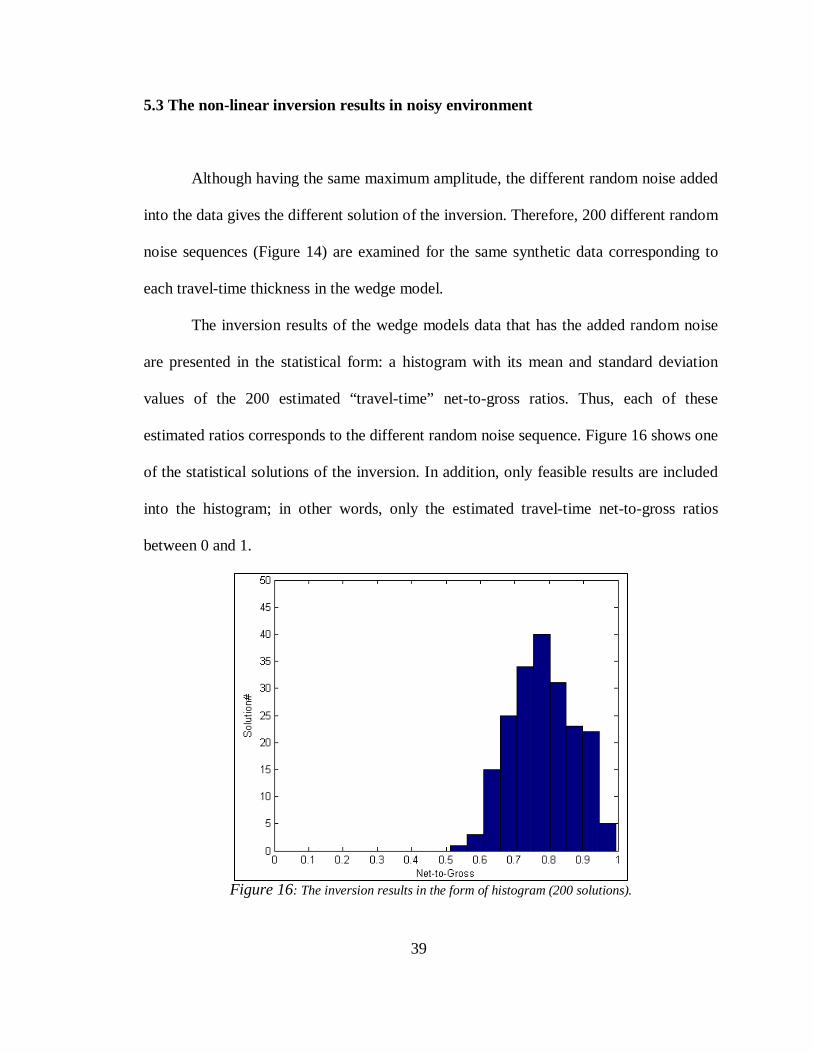
5.3 The non-linear inversion results in noisy environment

Although having the same maximum amplitude, the different random noise added

into the data gives the different solution of the inversion. Therefore, 200 different random

noise sequences (Figure 14) are examined for the same synthetic data corresponding to

each travel-time thickness in the wedge model.

The inversion results of the wedge models data that has the added random noise

are presented in the statistical form: a histogram with its mean and standard deviation

values of the 200 estimated “travel-time” net-to-gross ratios. Thus, each of these

estimated ratios corresponds to the different random noise sequence. Figure 16 shows one

of the statistical solutions of the inversion. In addition, only feasible results are included

into the histogram; in other words, only the estimated travel-time net-to-gross ratios

between 0 and 1.

Figure 16: The inversion results in the form of histogram (200 solutions).

40

Again, the three levels of the noise are examined by the inversion algorithm: 5%

(Figure 17a), 10% (Figure 17b), and 20 % (Figure 17c). Some inversion results are

consistent with the expectation: for each case, the smaller the level of the noise in the

model data, the smaller the standard deviation of the solution histogram.

However, one would expect that for each case, the smaller the thickness of the

mid layer (reservoir), the bigger the standard deviation of the solution histogram

becomes, as the destructive interference of the main and side lobes of the wavelets from

the reflections. This behavior of the solutions is not always true: when the travel-time

thickness of the reservoir is close to the tuning thickness (6.5 ms), the inversion algorithm

gives the solution with smaller standard deviation than the expected. This relation

between solutions is due to the constructive interference between the main and side lobe,

making the signal stronger.

16 ms 8 ms 1 ms 1/16 ms4 ms 2 ms 1/2 ms 1/4ms 1/8ms


0.7850 0.7650 0.7550 0.7525 0.7512 0.7506

Estimated “travel-time” Net/Gross (µ – mean ; � – standard deviation) : µ 0.778 0.749 0.743 0.802 0.803 0.799� 0.078 0.088 0.068 0.077 0.079 0.121

Note: only reasonable results are included, that is, from 0 to 1.

(a)

41



0.7850 0.7650 0.7550 0.7525 0.7512 0.7506


Note: only reasonable results are included, that is, from 0 to 1.

(b)



0.7850 0.7650 0.7550 0.7525 0.7512 0.7506


Note: only reasonable results are included, that is, from 0 to 1

(c) Figure 17: The wedge models with (a) 5%,

(b) 10%, and (c) 20 % of noise and the inversion results.

Similar conclusions can be made regarding the mean of the histograms: the

smaller the level of the noise in the model data, the smaller the difference between true

travel-time net-to-gross and the mean of the solutions. Likewise, the mean estimated for

42

the region of the tuning thickness is sometimes much closer to the true value then the

mean estimated for the region of the thicker thickness.

5.4 Inaccurate constraints

When the constraints are used in the inversion process, one question naturally

arises – What are the effects on the inversion results if the used constraints are

inaccurate? In the wedge-model synthetic case, two parameters are constrained by the

non-linear inversion algorithm – starting acoustic impedance of the underlying layer, and

travel-time thickness of the mid layer. Previously, the inversion of the wedge-models data

has been performed assuming that the constraints are accurate.

Before examining the effects of the inaccurate constraints, it is important to

analyze the method used to constraint the data. Here, the method of Lagrange multipliers

is used, whose mathematical background is explained in Section 3.4 (Non-linear

inversion using constraints). In the method, the solution of the non-linear inversion

problem corresponds to the optimization-function minimum satisfying the set of the

equality equations ( kFm = ). Each of the equality equations used in the optimization

procedure is associated with the Lagrange multiplier (�). The Lagrange multiplier is

crucial parameter in terms of understanding the effects of the constraint on the solution of

the inversion problem.

Implementing the previous discussion in the wedge model case, the starting

acoustic impedance of the underlying layer and the travel-time thickness of the mid layer

are constrained using accurate and inaccurate values to examine this phenomenon.

43

5.5 Inaccurate constraint – time-travel thickness

To examine the effects of inaccurate travel-time thickness values, which are

constrained within the developed algorithm, on the inversion results, the data from the

previous wedge models are used; thus, the model parameters values used in the modeling

algorithm are the same as in the previous wedge model examples (Section 5.1: The

choice of the model parameter values). However the data of only one thickness are

investigated; in this case (Figure 18), the data are created modeling the 1-ms travel-time

thickness. Thus, the synthetic trace corresponding to the 1-ms travel-time thickness in the

wedge model are inverted using the inaccurate constrained thickness: 16, 8, 4, 2, 1/2, 1/4,

1/8 and 1/16 ms. The net-to-gross ratios applying both theories – ray and effective

medium – are estimated as well as Lagrange multipliers of the corresponding constraint

equality equation that involves one accurate and several inaccurate travel-time thickness.

Figure 18: Inversion results using the inaccurate constraint – travel-time thickness.


True Net/Gross: EMT: 0.774RT: 0.751

Estimated Net/Gross: EMT: 0.508 0.317 0.422 0.533 0.774 >1 (4.8) >1(5.3) >1(31) >1(73)RT: 0.475 0.288 0.390 0.500 0.751 >1 (6.3) >1(7.1) >1(52) >1(124)

Lagrange multiplier value:10-6 10-6 10-11 10-13 10-23 10-8 10-8 10-6 10-6

44

First, regarding the estimated net-to-gross ratios, intuitively, the bigger the

discrepancy between the accurate and used thickness, the biggest the error between the

true and estimated net-to-gross ratio. Second, the Lagrange multiplier value associated

with the accurate travel-time thickness is closest to zero (10-23) comparing with those of

the inaccurate travel-time thickness.

This relation between the Lagrange multipliers of accurate and inaccurate

constraint equality equations suggests, keeping in mind the previous discussion about the

physical meaning of the multipliers (Section 3.4 Non-linear inversion including

constraints), that the travel-time thickness does not have to be constrained to have the

unique solution. Because the travel-time thickness is actually estimated using the same

set of data by spectral inversion and thus does not represent a priori information, it is not

surprise that this parameter does not have to be constrained in the inversion algorithm.

However, in the real example, the spectral inversion determined travel-time

thickness is going to be constrained and examined, as it is a mean of 1) biasing the

inversion in directions found to be desirable for interpretation purposes, 2) reducing the

dimension of initial-model space, and 3) determining the resample rate in the inversion

algorithm.

In addition, the net-to-gross ratios estimated are plotted as a function of the

constrained travel-time thickness (Figure 19). Clearly, the relations between these two

quantities are non-linear.

45

Figure 19: The net-to-gross ratios vs. the constrained travel-time thickness.

5.6 Inaccurate constraint - starting acoustic impedance

The same synthetic data are used to examine the effects of the inaccurately

constrained starting acoustic impedance of the overlying layer. However, in this case, the

assumption is that the travel-time thickness is known correctly, whereas the starting

acoustic impedance is constrained using one accurate and several inaccurate values

within the range from 4 to 8 10-6 SI. The net-to-gross ratios as well as Lagrange

multipliers values corresponding to the given constraints are estimated and calculated

(Figure 20), applying both ray and effective medium theories.

46

Figure 20: The inversion results using inaccurate constraint – starting acoustic impedance.

Again, here the bigger the error of constrained value, the bigger the error in

estimated results. However, here in a case of ray theory bound, the relation between the

constrained value and estimated net-to-gross ratio are linearly dependent, whereas the

relation, in a case of effective medium theory bound, is still non-linear but very close to

linear (Figure 21).

Speaking of the estimated Lagrange multipliers, regardless of the constrained

value, whether it is accurate (6.5) or not, their value are the same! These constant

multipliers suggest that all constraints have the equal “force” to change the minimum of

the objective function. In addition, the solution of the inversion is non-unique, as the

objective function does not have a single global miminum. Therefore, such a parameter

has to be constrained with a priori information to have a unique solution. Thus, in the

Estimated N/G:EMT: -0.147 0.188 0.492 0.774 1.038 1.289 1.528 RT: -0.124 0.168 0.459 0.751 1.043 1.335 1.627

Lagrange multiplier value:10-23 10-23 10-23 10-23 10-22 10-23 10-22

1 ms

True N/GEMT: 0.774RT: 0.751

I14.5 5.0 Ishale=5.5 I1=6.0 6.5 7.0 Isand= 7.5

47

real example (chapter 4. Real example), a starting acoustic impedance of one of the layers

is constrained using the value determined from the different technique – well logging.

Figure 21: The net-to-gross ratio vs. constrained starting acoustic impedance.

48

6. Synthetic example – Multi-layer case

In the previous example, wedge models, there were three assumptions limiting the

implementation of such an algorithm into the real case:

1) The number of layers is known (though it could be estimated from

spectral inversion).

2) Only three layers are used.

3) The synthetic data were generated using the actual parameterization

(unrealistic impedance profile).

Figure 22: Generating synthetic data to be used in the inversion.

Therefore, another synthetic has been investigated. In the synthetic case, all three

previous assumptions are excluded: that is, the number of layers is considered to be

unknown and arbitrary, and the data are more realistic by adding the uniform random

R.C.

*

a)

c)b)

49

function on the acoustic impedance profile before creating the reflection coefficient for

the synthetic data: on Figure 22, it is shown how the synthetic data has been created:

First, the arbitrary acoustic impedance profile has been created (Figure 22a); then, the

reflection coefficient profile is derived form the acoustic impedance profile, and finally,

by convolution of Ricker wavelet and the reflection coefficient profile (Figure 22b), the

data have been generated (Figure 22c).

Figure 23: Used constraints in the inversion.

Now, in the inversion procedure, as in the previous synthetic case, two parameters

have been constrained: a two-way travel-time thickness and starting acoustic impedance

of one of the layers. The assumption is that the former is known from the spectral

inversion and the latter is known from the well log interpretation. Their values are

respectively, 10 [ms] and 1.55 106 [kg/m3 m/s] in this case (Figure 23).

50

Figure 24: Ray theory “travel-time” net-to-gross ratio

as a function of a number of layers.

The inversion algorithm has investigated the affect of the different number of

layers. There is only one deterministic solution of net-to-gross ratio per the corresponding

number of layers for both theories – ray and effective medium (Figure 24 and 25,

respectively). These solutions of the inversion correspond to the global minimum solution

of objective function, that is, the smallest error between the synthetic data and estimated

data for each number of layers. The values of the objective function with the respect of

the number of layers used in the inversion are plotted on Figure 26: It is clear that the

more degrees of freedom used in the inversion, the less error between the actual and

predicted data. In addition, the values of the Lagrange multipliers associated with the

used constraints are shown on Figure 27.

Target

Estimated

51

Figure 25: Effective medium theory “travel-time” net-to-gross ratio


Overall, 5·107 trials were used to investigate different initial models with different

number of layers, assuming that the values are within the two standard deviations from

the mean of the uniform distribution, which is the input for the random sampling.

Figure 26: Objective function as a function of

a number of layers.

Target

Estimated

52

According to the values of net-to-gross ratio with the respect to the number of

layers for both theories, ray and effective medium (Figure 24 and 25, respectively), the

following can be concluded: by increasing the number of layers and thus degrees of

freedom, the estimated net-to-gross ratio approaches to the “true travel-time” net-to-gross

ratio. In this case the model that has thirteen layers gives the very good estimation of the

net-to-gross ratio (Figure 34). This behavior actually means that the average of acoustic

impedance using the thirteen layers are the same as the average of the target model.

Figure 27: Lagrange multipliers of two constrained parameters


This conclusion has been already seen in the inverse problems: the higher the

degrees of freedom, the better match between the actual and estimated model. For

example, it can be seen in designing matching filter in so-called Wiener least-square

filtering. The longer the length of the filter, the better matching between the input and

desired output (Robinson and Treitel, 2001).

53

On the other hand, it is interesting to mention that the best match for the

interpretation of the gradients gives the model that uses the only eight layers (Figure 29).

According to the results, objective function (Figure 26) and Lagrange multipliers that

correspond to the constraints (Figure 27) show abrupt drop in their value, at that point

where the solution should be used for geological interpretation.

The estimated models that correspond to the global minima for each of the

number of layers are show bellow (Figure 28-34).

Figure 28: Inversion solution using seven layers.

Target

Estimated

54

Figure 29: Inversion solution using eight layers.

Figure 30: Inversion solution using nine layers.

Target

Estimated

Target

Estimated

55

Figure 31: Inversion solution using ten layers.

Figure 32: Inversion solution using eleven layers.

Target

Estimated

Target

Estimated

56

Figure 33: Inversion solution using twelve layers.

Figure 34: Inversion solution using thirteen layers.

Target

Estimated

Target

Estimated

57

7. Real example – South Timbalier field

The South Timbalier field is located south from Louisiana in the Gulf of Mexico

(Figure 35). The available data from the field in the research are the post-migration stack

volume as well as geophysical well log data. Although there is available spectral

inversion volume for the area, it has to be discarded from the research as it was derived

using inaccurate synthetic ties from the previous study. Therefore, the algorithm is going

to use the constrained travel-time thickness from well logs rather then from the spectral

inversion results to estimate the feasibility of the developed algorithm.

Figure 35: South Timbalier field location (Stude, 1978).

The geological environment of South Timbalier field is typical for the Gulf of

Mexico: sedimentary basins with various salt domes and structures (Stude, 1978).

Because only one well at the location has the acoustic log data acquired, allowing

the accurate estimation of the seismic velocity of the formations, the research was limited

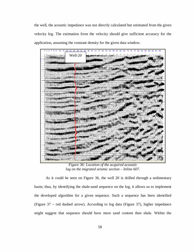
only to that well (Figure 36). In addition, because the density logs were not available in

58

the well, the acoustic impedance was not directly calculated but estimated from the given

velocity log. The estimation from the velocity should give sufficient accuracy for the

application, assuming the constant density for the given data window.

Figure 36: Location of the acquired acoustic log on the migrated seismic section – Inline 607.

As it could be seen on Figure 36, the well 20 is drilled through a sedimentary

basin; thus, by identifying the shale-sand sequence on the log, it allows us to implement

the developed algorithm for a given sequence. Such a sequence has been identified

(Figure 37 – red dashed arrow). According to log data (Figure 37), higher impedance

might suggest that sequence should have more sand content then shale. Within the

Well-20

59

sequence, the target layer has been defined (Figure 37 – black solid arrow). The target

layer is very thin; the two-way travel time thickness of the layer is 8 ms.

Figure 37: Well log data and synthetic tie in the well-20.

To efficiently apply the developed algorithm, it is crucial to have a good

correlation between the acoustic impedance profile and some net-to-gross ratio indicator,

such as gamma-ray or electrical self-potential (SP) well logs in the shale-sand sequence

of the interest. For the given well, only SP log is available, and there is a correlation

between the acoustic impedance (track 2) and self-potential log (track 1) in the area of

interest, making the algorithm applicable (Figure 37).

To test the feasibility and application of the research algorithm, the results of net-

to-gross ratio derived from the trace located nearest to the well are compared with the

60

results of net-to-gross ratio derived directly from the well log data. As a matter of fact,

the constrained data, that is, starting acoustic impedance of one of the layers and travel-

time thickness of the layer of interest, are used from the same well log data.

7.1 Estimating net-to-gross from the well logs

As it was stated before, the electric self-potential (SP) log can be used to

determine a net-to-gross ratio of a layer. The net-to-gross ratio is defined by the

following equation:

shss

shssz SSPSSP

SSPSP

h

hGrossNet

−−==/

where SP is electrical self-potential of the layer of interest, SSPss is a electrical self-

potential of clean send, and SSPsh is a electrical self-potential of clean shale. Using the

previous equation, the target layer in the research has the net-to-gross ratio of 0.85

(Figure 37 – black arrow). Because electric self-potential is measured in depth, such a

determination of the net-to-gross should represent “true” net-to-gross ratio.

In addition to estimating net-to-gross using the SP curve, the acoustic impedance

can be used to estimate travel-time net-to-gross ratio (Section 2.4 Calculating reservoir

travel-time net-to-gross ratio). Therefore, from equations 26 and 28, using ray and

effective medium theory respectively:

shss

shmeanrtt II

IIGrossNet

−−=/ and,

( )( )22

22

/shssmean

shmeanssemtt III

IIIGrossNet

−−

=

the calculated net-to-gross for the target layer is 0.87 and 0.89, respectively, which is

very close to the “true”, derived from SP curve – 0.85.

(64)

61

7.2 Estimating net-to-gross from the non-linear seismic inversion

Before the data are included into the developed algorithm to estimate travel-time

net-to-gross ratio, they have to be prepared with the following steps:

1) Perform the synthetic ties on the data in order to scale the amplitudes of

the trace to their absolute values. Here, STRATA (Hampson-Russell)

software has been used for the step. In this case, the correlation between

the synthetic and original trace has achieved the value of 0.82 (Figure

38a).

2) Determine the window of the trace that includes the layer of interest and

the anchor layer with the known value of starting acoustic impedance

throughout the area of interest. The good choice for the anchor layer

could be some shale sequence with a constant value throughout the

field. It should be kept in mind that the layers should not be affected by

the edge effect, that is, the length of the used window should be

sufficiently large (Figure 38b).

3) Apply the tapers on the edges of the trace window so that the edge

effects are reduced (Figure 38c).

4) Determine the values of the data to be constrained, that is, starting

acoustic impedance of the anchor layer and two-way travel-time

thickness of the layer of interest (Figure 38d).

62

5) Determine the acoustic impedance of the clean sand and clean shale.

These should be the minimum and maximum acoustic impedance

values in the shale and sand sequences, respectively for this case. Using

the well logs, the determined values for the clean shale and the clean

sand are 1.6 and 5.4 106 SI units, respectively.

Constrained time thickness –

�t = 8 ms

Constrained –I = 3.5 (10^6 SI)

a)

b) c)

d)

d)

Figure 38: Data preparation.

Now that data has been prepared the algorithm can be used to estimate the

acoustic impedance profile of the layer of interest and thus “travel-time” net-to-gross

ratio, assuming different number of layers in the model.

As it was previously stated in the multi-layer synthetic case, random sampling

technique has been used to investigate different initial models. The number of trials that

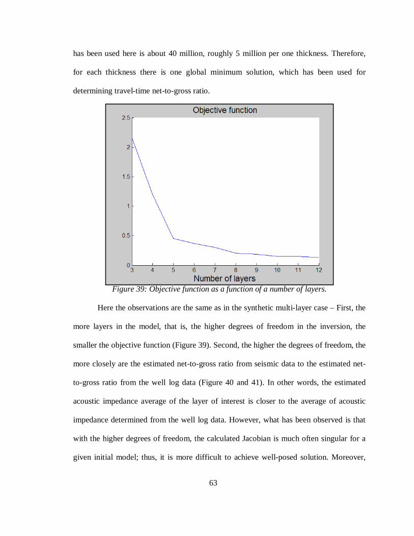
63

has been used here is about 40 million, roughly 5 million per one thickness. Therefore,

for each thickness there is one global minimum solution, which has been used for

determining travel-time net-to-gross ratio.

Figure 39: Objective function as a function of a number of layers.

Here the observations are the same as in the synthetic multi-layer case – First, the

more layers in the model, that is, the higher degrees of freedom in the inversion, the

smaller the objective function (Figure 39). Second, the higher the degrees of freedom, the

more closely are the estimated net-to-gross ratio from seismic data to the estimated net-

to-gross ratio from the well log data (Figure 40 and 41). In other words, the estimated

acoustic impedance average of the layer of interest is closer to the average of acoustic

impedance determined from the well log data. However, what has been observed is that

with the higher degrees of freedom, the calculated Jacobian is much often singular for a

given initial model; thus, it is more difficult to achieve well-posed solution. Moreover,

64

the computational time increases by increasing the number of layers, that is, model vector

dimension.

Figure 40: Ray theory travel-time net-to-gross ratio as a function of a number of layers.

In addition, the interesting question stayed unsolved - could we have known at the

beginning what is the sufficiently number of layers to be used in the inversion?

First, the answer to the previous question would have given the spectral inversion

technique, but as it is not accurate, we could not use it. Second, we can always do the

same scanning through different number of layers and see when the value of the net-to-

gross ratio (that is, acoustic impedance average) of the layer of interest is going to be

stable, and than use the result from the highest degrees of freedom. This approach is

feasible only if the computational time is not the issue.

65

Figure 41: Effective medium theory travel-time net-to-gross ratio as a function of a number of layers.

The results of the global minimum solution for even number of layers are shown

below (Figure 42, 43, 44, 45, and 46). The odd numbers of layers are skipped just for

simplicity. It should be stated that with the high degrees of freedom the estimated

acoustic impedance gradients of the layers are not interpretable. However, the general

trend of the estimated acoustic impedance gradients by the inversion has good match with

the regional trend of the well-measured acoustic impedance gradients (Figure 46).

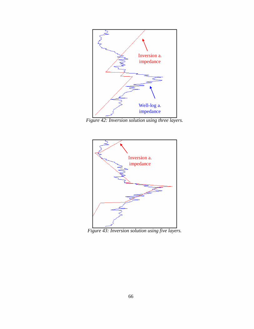
66

Figure 42: Inversion solution using three layers.

Figure 43: Inversion solution using five layers.

Well-log a. impedance

Inversion a. impedance


67

Figure 44: Inversion solution using seven layers.

Figure 45: Inversion solution using nine layers.



68

Figure 46: Inversion solution using eleven layers.


69

8. Conclusions

Constraining a priori information in the inversion algorithm clearly helped in

getting the unique solution of the seismic inversion problem, that is, achieving the global

minimum of objective function. It was found that one starting acoustic impedance in the

model had to be constrained in order to achieve global minimum of the objective

function. This conclusion was suggested using the synthetic wedge model (Section 5.4 –

Inaccurate constraints), where all constraint values, whether accurate or inaccurate, had

the same very weak magnitude of “force”, that is, Lagrange multiplier value, ~10-23,

making solution non-unique.

However, travel-time thickness of the layer of interest does not have to be

constrained to have a non-unique solution, but it is a mean for biasing the inversion in

directions found to be desirable for interpretation purposes. It was found in the same

synthetic wedge model that when the accurate thickness was constrained, a unique

minimum value of Lagrange multiplier was achieved ~10-23 magnitude comparing to the

other inaccurate values, making solution unique.

Furthermore, a random sampling technique, often called Monte Carlo sampling,

provides the way of scanning complete model space for the sufficiently good initial

model. Each of the solution for each of the initial model has been compared to get one

with the minimum error, thus, avoiding the local minimum, to be the solution of the

seismic inversion. In the real example at South Timbalier field, it was shown that twenty

million trials were sufficient to achieve satisfactory results. Further investigation could be

70

done to computationally determine optimal number of trials that should be used in an

inversion process.

The number of layers is crucial in the efficiency of the developed algorithm to get

accurate and/or stable result. The more number of layers involved in the inversion, that is,

the higher degrees of freedom in the inversion used in the inversion, the closer estimated

net-to-gross ratio to the actual net-to-gross ratio. On the other hand, the higher degrees of

freedom used in the inversion, the less stable is result, that is, the more difficult is to

achieve a non-singular Jacobian in the inversion, and the longer computational time of

the inversion. Here, the well-posed solutions, that is, the solutions with the non-singular

Jacobian, were achieved with the models with the number of layers between three and

twelve. The least-square error with three-layer model global solution was ~2.1, whereas

with twelve-layer model global solution was ~0.15, which is improvement in matching

actual with predicted data fourteen times.

Travel-time thickness net-to-gross ratio can be good indicator of the quality of

reservoir. When the correlation between the acoustic impedance and SP log has been

achieved, the estimated net-to-gross ratio gave very good estimation of the layer of

interest, even though the layer is below “conventional seismic resolution”, quarter of the

dominant wavelength. For the layer of interest in the research, using SP, the net-to-gross

ratio was estimated to be 0.85, whereas using the seismic inversion, the “travel-time” net-

to-gross was estimated to be 0.87 and 0.89 for ray and effective medium theories,

respectively.

However, the estimated gradients of the layers in general should not be used in

the interpretation, but on the other hand, the general trend of the estimated gradients has a

71

very good qualitative match with the actual one, that is, the one directly measured in the

well.

72

References

Backus, G. E., 1962, Long-wave elastic anisotropy produced by horizontal

layering: J. Geophys.Res., 67, 4427-4440.

Castagna, J. P., Sun, S., and Siegfried, R. W., 2003, Instantaneous spectral

analysis: Detection of low frequency shadows associated with

hydrocarbons: The Leading Edge, 22, 2, 120-127.

Chung, H., and Lawton, D. C., 1995, Frequency characteristics of seismic

reflections from thin beds: Canadian Journal of Exploration Geophysicists,

31, 32–37.

Cooke, D., and Schneider, W., 1983, Generalized linear inversion of reflection

seismic data: Geophysics, 48, 665-676.

Deitel, H., M., and Deitel, P., J., 2005, C++ How to Program, Fifth Edition,

Prentice Hall of India.

Gardner, G.H.F., Gardner, L.W., and Gregory, A.R., 1974, Formation Velocity

and Density – The Diagnostic Basics for Stratigraphic Traps: Geophysics,

39, 770-780.

Jensen, S., 2004, An introduction to Lagrange multipliers: http://www.slimy.com/

~steuardb/ tutorials/Lagrange.html.

Karabulut, H., 2006, The physical meaning of Lagrange multipliers: European

Journal of Physics, 27, 709-718.

Keilis-Borok,V. J., and Yanovskaya, T. B., 1967. Inverse problems of seismology

(structural review): Geophys. J. Royal Astr. Soc., 13, 223–234.

73

Madsen K., Nielsen H.B., and Tingleff, O., 2004, Methods for Non-Linear Lest-

Squares Problems, Denmark Technical University.

Marfurt, K. J. and Kirlin, R. L., 2001, Narrow-band spectral analysis and thin-bed

tuning: Geophysics, 66, 1274-1283.

Marion, D., Mukerji, T., and Mavko, G., 1994, Scale effects on velocity

dispersion: From ray to effective theories in stratified media: Geophysics,

59, 1613-1619.

Marquardt, D.W., 1963. An algorithm for least-squares estimation of nonlinear

parameters: J. Soc. Indust. Appl. Math., 11, 431–441.

Menke, W., 1984, Geophysical data analyses: discrete inverse theory: Academic

Press, Inc., New York.

Partyka, G., 2006, Spectral inversion to estimate the net-to-gross ratio, SEG

Meeting – Net-to-gross ratio workshop, Houston.

Partyka, G., Gridley, J. and Lopez, J., 1999, Interpretational applications of

spectral decomposition in reservoir characterization: The Leading Edge,

22, 3, 353-360.

Press, F., 1968. Earth models obtained by Monte-Carlo inversion: J. Geophys.

Res., 73, 16, 5223–5234.

Press, F., 1971. An introduction to earth structure and seismotectonics,

Proceedings of the International School of Physics Enrico Fermi, Course

L, Mantle and Core in Planetary Physics, Coulomb, J., and Caputo, M.

(editors), Academic Press, New York.

74

Reuss, A., 1929. Berechnung der fliessgrense von mischkristallen auf grund der

plastizitatbedingung fur einkristalle., Zeitschrift für Angewandte

Mathematik aus Mechnik.

Richardson R. and Zandt G., 2005, Inverse Problems in Geophysics, Department

of Geosciences, University of Arizona.

Russell, B., 1988, Introduction to Seismic Inversion Methods: SEG, Course Notes

Series, 2.

Robinson, E. A., and Treitel, S., 2001, Geophysical Signal Analysis, SEG, Tulsa

Sheriff, R., 2002, Encyclopedic Dictionary of Applied Geophysics: Society of

Exploration Geophysicists, Tulsa.

Stude, G. R., 1978, Depositional environments of the Gulf of Mexico South

Timbalier block 54 salt dome and salt dome growth models: Transactions-

Gulf Coast Association of Geological Societies, 28, 627-646.

Tarantola, A., 2005, Inverse Problem Theory and Model Parameter Estimation:

SIAM, Philadelphia.

Treitel, S., Lines, L., and Ruckgaber, G., 1993, Geophysical Inversion and

Applications: SEG and Memorial University.

Voigt, W., 1910, Lehrbuch Der Krystallphysic, Teubner, Leipzig.

Von Neumann, J., 1947, Letter to Stanislaw Ulam.

Widess, M. B, 1973, How thin is a thin bed: Geophysics, 38, 1176-1180.

Wikipedia, 2006, The Free Encyclopedia: Uniform distribution (continuous):

http://en.wikipedia.org/wiki/Uniform_distribution_(continuous).

75

Wyllie, M. R. J., Gregory, A. R., and Gardner, L. W., 1956, Elastic wave

velocities in heterogeneous and porous media: Geophysics, 21, 41-70.

constrained non-linear seismic inversion - allied geophysics

Documents