an overview of full-waveform inversion in exploration ... · pdf filean overview of...

A

J

pme1avsgapiodfm

g

©

GEOPHYSICS, VOL. 74, NO. 6 �NOVEMBER-DECEMBER 2009�; P. WCC127–WCC152, 15 FIGS., 1 TABLE.10.1190/1.3238367

n overview of full-waveform inversion in exploration geophysics

. Virieux1 and S. Operto2

wsnidttrTiqsn�t

ABSTRACT

Full-waveform inversion �FWI� is a challenging data-fittingprocedure based on full-wavefield modeling to extract quantita-tive information from seismograms. High-resolution imaging athalf the propagated wavelength is expected. Recent advances inhigh-performance computing and multifold/multicomponentwide-aperture and wide-azimuth acquisitions make 3D acousticFWI feasible today. Key ingredients of FWI are an efficient for-ward-modeling engine and a local differential approach, inwhich the gradient and the Hessian operators are efficiently esti-mated. Local optimization does not, however, prevent conver-gence of the misfit function toward local minima because of thelimited accuracy of the starting model, the lack of low frequen-cies, the presence of noise, and the approximate modeling of the

vps

httsiio�pctemc

d 8 Julyectonop

la Côte

WCC12

Downloaded 04 Dec 2009 to 193.50.85.151. Redistribution subject to

ave-physics complexity. Different hierarchical multiscaletrategies are designed to mitigate the nonlinearity and ill-posed-ess of FWI by incorporating progressively shorter wavelengthsn the parameter space. Synthetic and real-data case studies ad-ress reconstructing various parameters, from VP and VS veloci-ies to density, anisotropy, and attenuation. This review attemptso illuminate the state of the art of FWI. Crucial jumps, however,emain necessary to make it as popular as migration techniques.he challenges can be categorized as �1� building accurate start-

ng models with automatic procedures and/or recording low fre-uencies, �2� defining new minimization criteria to mitigate theensitivity of FWI to amplitude errors and increasing the robust-ess of FWI when multiple parameter classes are estimated, and3� improving computational efficiency by data-compressionechniques to make 3D elastic FWI feasible.

INTRODUCTION

Seismic waves bring to the surface information gathered on thehysical properties of the earth. Since the discovery of modern seis-ology at the end of the 19th century, the main discoveries have aris-

n from using traveltime information �Oldham, 1906; Gutenberg,914; Lehmann, 1936�. Then there was a hiatus until the 1980s formplitude interpretation, when global seismic networks could pro-ide enough calibrated seismograms to compute accurate syntheticeismograms using normal-mode summation. Differential seismo-rams estimated through the Born approximation have been useds perturbations for matching long-period seismograms, which canrovide high-resolution upper-mantle tomography �Gilbert and Dz-ewonski, 1975; Woodhouse and Dziewonski, 1984�. The sensitivityr Fréchet derivative matrix, i.e., the partial derivative of seismicata with respect to the model parameters, is explicitly estimated be-ore proceeding to inversion of the linearized system. The normal-ode description allows a limited number of parameters to be in-

Manuscript received by the Editor 7 June 2009; revised manuscript receive1Université Joseph Fourier, Laboratoire de Géophysique Interne et T

renoble.fr.2Université Nice-SophiaAntipolis, Géoazur, CNRS, IRD, Observatoire de2009 Society of Exploration Geophysicists.All rights reserved.

erted �a few hundred parameters�, which makes the optimizationrocedure feasible through explicit sensitivity matrix estimation inpite of the high number of seismograms.

Meanwhile, exploration seismology has taken up the challenge ofigh-resolution imaging of the subsurface by designing dense, mul-ifold acquisition systems. Construction of the sensitivity matrix isoo prohibitive because the number of parameters exceed 10,000. In-tead, another road has been taken to perform high-resolution imag-ng. Using the exploding-reflector concept, and after some kinemat-c corrections, amplitude summation has provided detailed imagesf the subsurface for reservoir determination and characterizationClaerbout, 1971, 1976�. The sum of the traveltimes from a specificoint of the interface toward the source and the receiver should coin-ide with the time of large amplitudes in the seismogram. The reflec-ivity as an amplitude attribute of related seismic traces at the select-d point of the reflector provides the migrated image needed for seis-ic stratigraphic interpretation. Although migration is more a con-

ept for converting seismic data recorded in the time-space domain

2009; published online 3 December 2009.hysique, CNRS, IRD, Grenoble, France. E-mail: [email protected]

d’Azur, Villefranche-sur-mer, France. E-mail: [email protected].

7

SEG license or copyright; see Terms of Use at http://segdl.org/

irmt

la1ttDmraibaVs2ts

Lptrfbaeaepp�lfsset

tbim1p2aaebBmsasp

aewapzmemsnm

bveiisvo�pta�M1

nflrmtmsp�Tfarl

cFattawnRpis2

f

WCC128 Virieux and Operto

nto images of physical properties, we often refer to it as the geomet-ic description of the short wavelengths of the subsurface.Avelocityacromodel or background model provides the kinematic informa-

ion required to focus waves inside the medium.The limited offsets recorded by seismic reflection surveys and the

imited-frequency bandwidth of seismic sources make seismic im-ging poorly sensitive to intermediate wavelengths �Jannane et al.,989�. This is the motivation behind a two-step workflow: constructhe macromodel using kinematic information, and then the ampli-ude projection using different types of migrations �Claerbout andoherty, 1972; Gazdag, 1978; Stolt, 1978; Baysal et al., 1983; Yil-az, 2001; Biondi and Symes, 2004�. This procedure is efficient for

elatively simple geologic targets in shallow-water environments,lthough more limited performances have been achieved for imag-ng complex structures such as salt domes, subbasalt targets, thrustelts, and foothills. In complex geologic environments, building anccurate velocity background model for migration is challenging.arious approaches for iterative updating of the macromodel recon-truction have been proposed �Snieder et al., 1989; Docherty et al.,003�, but they remain limited by the poor sensitivity of the reflec-ion seismic data to the large and intermediate wavelengths of theubsurface.

Simultaneous with the global seismology inversion scheme,ailly �1983� and Tarantola �1984� recast the migration imagingrinciple of Claerbout �1971, 1976� as a local optimization problem,he aim of which is least-squares minimization of the misfit betweenecorded and modeled data. They show that the gradient of the misfitunction along which the perturbation model is searched can be builty crosscorrelating the incident wavefield emitted from the sourcend the back-propagated residual wavefields. The perturbation mod-l obtained after the first iteration of the local optimization looks likemigrated image obtained by reverse-time migration. One differ-

nce is that the seismic wavefield recorded at the receiver is backropagated in reverse time migration, whereas the data misfit is backropagated in the waveform inversion of Lailly �1983� and Tarantola1984�. When added to the initial velocity, the velocity perturbationsead to an updated velocity model, which is used as a starting modelor the next iteration of minimizing the misfit function. The impres-ive amount of data included in seismograms �each sample of a timeeries must be considered� is involved in gradient estimation. Thisstimation is performed by summation over sources, receivers, andime.

Waveform-fitting imaging was quite computer demanding at thatime, even for 2D geometries �Gauthier et al., 1986�. However, it haseen applied successfully in various studies using forward-model-ng techniques such as reflectivity techniques in layered media �Kor-endi and Dietrich, 1991�, finite-difference techniques �Kolb et al.,986; Ikelle et al., 1988; Crase et al., 1990; Pica et al., 1990; Djik-éssé and Tarantola, 1999�, finite-element methods �Choi et al.,008�, and extended ray theory �Cary and Chapman, 1988; Koren etl., 1991; Sambridge and Drijkoningen, 1992�. A less computation-lly intensive approach is achieved by Jin et al. �1992� and Lambarét al. �1992�, who establish the theoretical connection between ray-ased generalized Radon reconstruction techniques �Beylkin, 1985;leistein, 1987; Beylkin and Burridge, 1990� and least-squares opti-ization �Tarantola, 1987�. By defining a specific norm in the data

pace, which varies from one focusing point to the next, they wereble to recast the asymptotic Radon transform as an iterative least-quares optimization after diagonalizing the Hessian operator. Ap-lications on 2D synthetic data and real data are provided �Thierry et


l., 1999b; Operto et al., 2000� and 3D extension is possible �Thierryt al., 1999a; Operto et al., 2003� because of efficient asymptotic for-ard modeling �Lucio et al., 1996�. Because the Green’s functions

re computed in smoothed media with the ray theory, the forwardroblem is linearized with the Born approximation, and the optimi-ation is iterated linearly, which means the background model re-ains the same over the iterations. These imaging methods are gen-

rally called migration/inversion or true-amplitude prestack depthigration �PSDM�. The main difference with the waveform-inver-

ion methods we describe is that the smooth background model doesot change over iterations and only the single scattered wavefield isodeled by linearizing the forward problem.Alternatively, the full information content in the seismogram can

e considered in the optimization. This leads us to full-waveform in-ersion �FWI�, where full-wave equation modeling is performed atach iteration of the optimization in the final model of the previousteration.All types of waves are involved in the optimization, includ-ng diving waves, supercritical reflections, and multiscattered wavesuch as multiples. The techniques used for the forward modelingary and include volumetric methods such as finite-element meth-ds �Marfurt, 1984; Min et al., 2003�, finite-difference methodsVirieux, 1986�, finite-volume methods �Brossier et al., 2008�, andseudospectral methods �Danecek and Seriani, 2008�; boundary in-egral methods such as reflectivity methods �Kennett, 1983�; gener-lized screen methods �Wu, 2003�; discrete wavenumber methodsBouchon et al., 1989�; generalized ray methods such as WKBJ andaslov seismograms �Chapman, 1985�; full-wave theory �de Hoop,

960�; and diffraction theory �Klem-Musatov andAizenberg, 1985�.FWI has not been recognized as an efficient seismic imaging tech-

ique because pioneering applications were restricted to seismic re-ection data. For short-offset acquisition, the seismic wavefield isather insensitive to intermediate wavelengths; therefore, the opti-ization cannot adequately reconstruct the true velocity structure

hrough iterative updates. Only when a sufficiently accurate initialodel is provided can waveform-fitting converge to the velocity

tructure through such updates. For sampling the initial model, so-histicated investigations with global and semiglobal techniquesKoren et al., 1991; Jin and Madariaga, 1993, 1994; Mosegaard andarantola, 1995; Sambridge and Mosegaard, 2002� have been per-ormed. The rather poor performance of these investigations thatrises from insensitivity to intermediate wavelengths has led manyesearchers to believe that this optimization technique is not particu-arly efficient.

Only with the benefit of long-offset and transmission data to re-onstruct the large and intermediate wavelengths of the structure hasWI reached its maturity as highlighted by Mora �1987, 1988�, PrattndWorthington �1990�, Pratt et al. �1996�, and Pratt �1999�. FWI at-empts to characterize a broad and continuous wavenumber spec-rum at each point of the model, reunifying macromodel buildingnd migration tasks into a single procedure. Historical crosshole andide-angle surface data examples illustrate the capacity of simulta-eous reconstruction of the entire spatial spectrum �e.g., Pratt, 1999;avaut et al., 2004; Brenders and Pratt, 2007a�. However, robust ap-lication of FWI to long-offset data remains challenging because ofncreasing nonlinearities introduced by wavefields propagated overeveral tens of wavelengths and various incidence angles �Sirgue,006�.Here, we consider the main aspects of FWI. First, we review the

orward-modeling problem that underlies FWI. Efficient numerical


mp

bc1Hrbe

hbTtomcttFWi

vare

lRm

tmt�apbm2

w�wshaatwr�

tha

lt

wpm2

attmfpHafp2

t2iptoprtttpt

od2rwiemc

fifti2twwmafl

Full-waveform inversion WCC129

odeling of the full seismic wavefield is a central issue in FWI, es-ecially for 3D problems.In the second part, we review the main theoretical aspects of FWI

ased on a least-squares local optimization approach. We follow theompact matrix formalism for its simplicity �Pratt et al., 1998; Pratt,999�, which leads to a clear interpretation of the gradient and theessian of the objective function. Once the gradient is estimated, we

eview different optimization algorithms used to compute the pertur-ation model. We conclude the methodology section by the sourcestimation problem in FWI.

In the third part, we review some key features of FWI. First, weighlight the relationships between the experimental setup �sourceandwidth, acquisition geometry� and the spatial resolution of FWI.he resolution analysis provides the necessary guidelines to design

he multiscale FWI algorithms required to mitigate the nonlinearityf FWI. We discuss the pros and cons of the time and frequency do-ains for efficient multiscale algorithms. We provide a few words

oncerning the parallel implementation of FWI techniques becausehese are computer demanding. Then we review some alternatives tohe least-squares criterion and the Born linearization. A key issue ofWI is the initial model from which the local optimization is started.e also discuss several tomographic approaches to building a start-

ng model.In the fourth part, we review the main case studies of FWI subdi-

ided into three categories of case studies: acoustic, multiparameter,nd three dimensional. Finally, we discuss the future challengesaised by the revival of interest in FWI that has been shown by thexploration and the earthquake-seismology communities.

THE FORWARD PROBLEM

Let us first introduce the notations for the forward problem, name-y, modeling the full seismic wavefield. The reader is referred toobertsson et al. �2007� for an up-to-date series of publications onodern seismic-modeling methods.We use matrix notations to denote the partial-differential opera-

ors of the wave equation �Marfurt, 1984; Carcione et al., 2002�. Theost popular direct method to discretize the wave equation in the

ime and frequency domains is the finite-difference methodVirieux, 1986; Levander, 1988; Graves, 1996; Operto et al., 2007�,lthough more sophisticated finite-element or finite-volume ap-roaches can be considered. This is especially true when accurateoundary conditions through unstructured meshes must be imple-ented �e.g., Komatitsch and Vilotte, 1998; Dumbser and Kaser,

006�.In the time domain, we have

M�x�d2u�x,t�

dt2�A�x�u�x,t��s�x,t�, �1�

here M and A are the mass and the stiffness matrices, respectivelyMarfurt, 1984�. The source term is denoted by s and the seismicavefield by u. In the acoustic approximation, u generally repre-

ents pressure, although in the elastic case u generally representsorizontal and vertical particle velocities. The time is denoted by tnd the spatial coordinates by x. Equation 1 generally is solved withn explicit time-marching algorithm: The value of the wavefield at aime step �n�1� at a spatial position is inferred from the value of theavefields at previous time steps. Implicit time-marching algo-

ithms are avoided because they require solving a linear systemMarfurt, 1984�. If both velocity and stress wavefields are helpful,


he system of second-order equations can be recast as a first-orderyperbolic velocity-stress system by incorporating the necessaryuxiliary variables �Virieux, 1986�.

In the frequency domain, the wave equation reduces to a system ofinear equations; the right-hand side is the source and the solution ishe seismic wavefield. This system can be written compactly as

B�x,��u�x,��s�x,��, �2�

here B is the impedance matrix �Marfurt, 1984�. The sparse com-lex-valued matrix B has a symmetric pattern, although it is not sym-etric because of absorbing boundary conditions �Hustedt et al.,

004; Operto et al., 2007�.Equation 2 can be solved by a decomposition of B such as lower

nd upper �LU� triangular decomposition, leading to direct-solverechniques. The advantage of the direct-solver approach is that oncehe decomposition is performed, equation 2 is efficiently solved forultiple sources using forward and backward substitutions �Mar-

urt, 1984�. The direct-solver approach is efficient for 2D forwardroblems �Jo et al., 1996; Stekl and Pratt, 1998; Hustedt et al., 2004�.owever, the time and memory complexities of LU factorization

nd its limited scalability on large-scale distributed memory plat-orms prevent use of the approach for large-scale 3D problems �i.e.,roblems involving more than 10 million unknowns; Operto et al.,007�.Iterative solvers provide an alternative approach for solving the

ime-harmonic wave equation �Riyanti et al., 2006, 2007; Plessix,007; Erlangga and Herrmann, 2008�. Iterative solvers currently aremplemented with Krylov subspace methods �Saad, 2003� that arereconditioned by solving the dampened time-harmonic wave equa-ion. The solution of the dampened wave equation is computed withne cycle of a multigrid. The main advantage of the iterative ap-roach is the low memory requirement, although the main drawbackesults from a difficulty to design an efficient preconditioner becausehe impedance matrix is indefinite. To our knowledge, the extensiono elastic wave equations still needs to be investigated. As for theime-domain approach, the time complexity of the iterative ap-roach increases linearly with the number of sources in contrast tohe direct-solver approach.

An intermediate approach between the direct and iterative meth-ds consists of a hybrid direct-iterative approach based on a domainecomposition method and the Schur complement system �Saad,003; Sourbier et al., 2008�. The iterative solver is used to solve theeduced Schur complement system, the solution of which is theavefield at interface nodes between subdomains. The direct solver

s used to factorize local impedance matrices that are assembled onach subdomain. Briefly, the hybrid approach provides a compro-ise in terms of memory savings and multisource-simulation effi-

iency between the direct and the iterative approaches.The last possible approach to compute monochromatic wave-

elds is to perform the modeling in the time domain and extract therequency-domain solution either by discrete Fourier transform inhe loop over the time steps �Sirgue et al., 2008� or by phase-sensitiv-ty detection once the steady-state regime is reached �Nihei and Li,007�. One advantage of the approach based on the discrete Fourierransform is that an arbitrary number of frequencies can be extractedithin the loop over time steps at minimal extra cost. Second, timeindowing can be easily applied, which is not the case when theodeling is performed in the frequency domain. Time windowing

llows the extraction of specific arrivals for FWI �early arrivals, re-ections, PS converted waves�, which is often useful to mitigate the


n�

pttipft

�bai�

rtcTtsntsppf

tccg

b2tG

i

mltS

bsstetTd

afivsmaTtaitflm

Ti

w

ftotmv

oIdif

t

Ti

Trg


onlinearity of the inversion by judicious data preconditioningSears et al., 2008; Brossier et al., 2009a�.

Among all of these possible approaches, the iterative-solver ap-roach theoretically has the best time complexity �here, “complexi-y” denotes how the computational cost of an algorithm grows withhe size of the computational domain� if the number of iterations isndependent of the frequency �Erlangga and Herrmann, 2008�. Inractice, the number of iterations generally increases linearly withrequency. In this case, the time complexities of the time-domain andhe iterative-solver approach are equivalent �Plessix, 2007�.

The reader is referred to Plessix �2007, 2009� and Virieux et al.2009� for more detailed complexity analyses of seismic modelingased on different numerical approaches. A discussion on the prosnd cons of time-domain versus frequency-domain seismic model-ng with application to FWI is also provided in Vigh and Starr2008b� and Warner et al. �2008�.

Source implementation is an important issue in FWI. The spatialeciprocity of Green’s functions can be exploited in FWI to mitigatehe number of forward problems if the number of receivers is signifi-antly smaller than the number of sources �Aki and Richards, 1980�.he reciprocity of Green’s functions also allows matching data emit-

ed by explosions and recorded by directional sensors, with pressureynthetics computed for directional forces �Operto et al., 2006�. Ofote, the spatial reciprocity is satisfied theoretically for the unidirec-ional sensor and the unidirectional impulse source. However, thepatial reciprocity of the Green’s functions can also be used for ex-losive sources by virtue of the superposition principle. Indeed, ex-losions can be represented by double dipoles or, in other words, byour unidirectional impulse sources.

Afinal comment concerns the relationship between the discretiza-ion required to solve the forward problem and that required to re-onstruct the physical parameters. Often during FWI, these two dis-retizations are identical, although it is recommended that the fin-erprint of the forward problem be kept minimal in FWI.The properties of the subsurface that we want to quantify are em-

edded in the coefficients of matrices M, A, or B of equations 1 and. The relationship between the seismic wavefield and the parame-ers is nonlinear and can be written compactly through the operator, defined as

u�G�m� �3�

n the time domain or in the frequency domain.

FWI AS A LEAST-SQUARES LOCALOPTIMIZATION

We follow the simplest view of FWI based on the so-called lengthethod �Menke, 1984�. For information on probabilistic maximum

ikelihood or generalized inverse formulations, the reader is referredo Menke �1984�, Tarantola �1987�, Scales and Smith �1994�, anden and Stoffa �1995�.We define the misfit vector �d�dobs�dcal�m� of dimension N

y the differences at the receiver positions between the recordedeismic data dobs and the modeled seismic data dcal�m� for eachource-receiver pair of the seismic survey. Here, dcal can be related tohe modeled seismic wavefield u by a detection operator R, whichxtracts the values of the wavefields computed in the full computa-ional domain at the receiver positions for each source: dcal�Ru.he model m represents some physical parameters of the subsurfaceiscretized over the computational domain.


In the simplest case corresponding to the monoparameter acousticpproximation, the model parameters are the P-wave velocities de-ned at each node of the numerical mesh used to discretize the in-erse problem. In the extreme case, the model parameters corre-pond to the 21 elastic moduli that characterize linear triclinic elasticedia, the density, and some memory variables that characterize the

nelastic behavior of the subsurface �Toksöz and Johnston, 1981�.he most common discretization consists of projection of the con-

inuous model of the subsurface on a multidimensional Dirac comb,lthough a more complex basis can be considered �see Appendix An Pratt et al. �1998� for a discussion on alternative parameteriza-ions�. We define a norm C�m� of this misfit vector �d, which is re-erred to as the misfit function or the objective function.We focus be-ow on the least-squares norm, which is easier to manipulate mathe-atically �Tarantola, 1987�. Other norms are discussed later.

he Born approximation and the linearization of thenverse problem

The least-squares norm is given by

C�m��1

2�d†�d, �4�

here † denotes the adjoint operator �transpose conjugate�.In the time domain, the implicit summation in equation 4 is per-

ormed over the number of source-channel pairs and the number ofime samples in the seismograms, where a channel is one componentf a multicomponent sensor. In the frequency domain, the summa-ion over frequencies replaces that over time. In the time domain, theisfit vector is real valued; in the frequency domain, it is complex

alued.The minimum of the misfit function C�m� is sought in the vicinity

f the starting model m0. The FWI is essentially a local optimization.n the framework of the Born approximation, we assume that the up-ated model m of dimension M can be written as the sum of the start-ng model m0 plus a perturbation model �m:m�m0��m. In theollowing, we assume that m is real valued.

A second-order Taylor-Lagrange development of the misfit func-ion in the vicinity of m0 gives the expression

C�m0��m��C�m0�� j�1

M�C�m0�

�mj�mj

�1

2 �j�1

M

�k�1

M� 2C�m0��mj�mk

�mj�mk�O�m3� .

�5�

aking the derivative with respect to the model parameter ml resultsn

�C�m��ml

��C�m0�

�ml� �

j�1

M� 2C�m0��mj�ml

�mj . �6�

he minimum of the misfit function in the vicinity of point m0 iseached when the first derivative of the misfit function vanishes.Thisives the perturbation model vector:

�m�� 2C�m0��m2 ��1�C�m0�

�m. �7�


sTtOf�eIaw

Ns

B

g

we

wtps

mt

I�m

Tlc

z

mnmpH

polpav

w�

ttmrg

Tot

wfTbobe�

�b�

tgmmTalt


The perturbation model is searched in the opposite direction of theteepest ascent �i.e., the gradient� of the misfit function at point m0.he second derivative of the misfit function is the Hessian; it defines

he curvature of the misfit function at m0. Of note, the error term�m3� in equation 5 is zero when the misfit function is a quadratic

unction of m. This is the case for linear forward problems such as uG.m. In this case, the expression of the perturbation model of

quation 7 gives the minimum of the misfit function in one iteration.n FWI, the relationship between the data and the model is nonlinearnd the inversion needs to be iterated several times to converge to-ard the minimum of the misfit function.

ormal equations: The Newton, Gauss-Newton, andteepest-descent methods

asic equations

The derivative of C�m� with respect to the model parameter ml

ives

�C�m��ml

��1

2 �i�1

N �� dcali

�ml��dobsi

�dcali�*

� �dobsi�dcali

��dcali

*

�ml�

��i�1

N

R�� dcali

�ml�*

�dobsi�dcali

��, �8�

here the real part and the conjugate of a complex number are denot-d by R and *, respectively. In matrix form, equation 8 translates to

�Cm��C�m�

�m��R�� dcal�m�

�m�†

�dobs�dcal�m��R�J†�d, �9�

here J is the sensitivity or the Fréchet derivative matrix. In equa-ion 9, �Cm is a vector of dimension M. Taking m�m0 in equation 9rovides the descent direction along which the perturbation model isearched in equation 7.

Differentiation of the gradient expression 8, with respect to theodel parameters gives the following expression in matrix form for

he Hessian �see Pratt et al. �1998� for details�:

� 2C�m0��m2 �R�J0

†J0�R� �J0t

�mt ��d0* . . .�d0

*�� . �10�

nserting the expression of the gradient �equation 9� and the Hessianequation 10� into equation 7 gives the following for the perturbationodel:

�m��R�J0†J0�

�J0t

�mt ��d0* . . .�d0

*��1

R�J0†�d0 .

�11�

he method solving the normal equations, e.g., equation 11, general-y is referred to as the Newton method, which is locally quadraticallyonvergent.

For linear problems �d�G.m�, the second term in the Hessian isero because the second-order derivative of the data with respect to


odel parameters is zero. Most of the time, this second-order term iseglected for nonlinear inverse problems. In the following, the re-aining term in the Hessian, i.e., Ha�J0

†J0, is referred to as the ap-roximate Hessian.The method which solves equation 11 when only

a is estimated is referred to as the Gauss-Newton method.Alternatively, the inverse of the Hessian in equation 11 can be re-

laced by a scalar �, the so-called step length, leading to the gradientr steepest-descent method. The step length can be estimated by aine-search method, for which a linear approximation of the forwardroblem is used �Gauthier et al., 1986; Tarantola, 1987�. In the linearpproximation framework, the second-order Taylor-Lagrange de-elopment of the misfit function gives

C�m�� C�m0��C�m��C�m� �C�m0��

�1

2�2Ha�m��C�m0� �C�m0��,

�12�here we assume a model perturbation of the form �m� �C�m0�. In equation 12, we replace the second-order deriva-

ive of the misfit function by the approximate Hessian in the seconderm on the right-hand side. Inserting the expression of the approxi-ate Hessian Ha into the previous expression, zeroing the partial de-

ivative of the misfit function with respect to �, and using m�m0

ives

� ��C�m0� �C�m0��

��Jt�m0��C�m0� Jt�m0��C�m0��. �13�

he term Jt�m0��C�m0� is computed conventionally using a first-rder-accurate finite-difference approximation of the partial deriva-ive of G,

�G�m0��m

�C�m0��1

��G�m0��C�m0��G�m0��,

�14�

ith a small parameter �. Estimation of � requires solving an extraorward problem per shot for the perturbed model m0��C�m0�.his line-search technique is extended to multiple-parameter classesy Sambridge et al. �1991� using a subspace approach. In this case,ne forward problem must be solved per parameter class, which cane computationally expensive. Alternatively, the step length can bestimated by parabolic interpolation through three points, ��,C�m0

� �C�m0��. The minimum of the parabola provides the desired. In this case, two extra forward problems per shot must be solvedecause we already have a third point corresponding to �0,C�m0��see Figure 1 in Vigh et al. �2009� for an illustration�.

Pratt et al. �1998� illustrate how quality and rate of convergence ofhe inversion depend significantly on the Newton, Gauss-Newton, orradient method used. Importantly, they show how the gradientethod can fail to converge toward an acceptable model, howeverany iterations, unlike the Newton and Gauss-Newton methods.hey interpret this failure as the result of the difficulty of estimatingreliable step length. However, gradient methods can be significant-

y improved by scaling �i.e., dividing� the gradient by the diagonalerms of H or of the pseudo-Hessian �Shin et al., 2001a�.
a

N

retar

joa

IW��e

N

p�atovo

aikmenarqtFepbmo

N

G�monut

�fng

f�ecc

R

ia�t

wWfotvsdsl�fiar�

nt

wT

Ewste�

t


umerical algorithms: The conjugate-gradient method

Over the last decade, the most popular local optimization algo-ithm for solving FWI problems was based on the conjugate-gradi-nt method �Mora, 1987; Tarantola, 1987; Crase et al., 1990�. Here,he model is updated at the iteration n in the direction of p�n�, which islinear combination of the gradient at iteration n, �C�n�, and the di-

ection p�n�1�:

p�n�� Cn�� n�p�n�1�. �15�

The scalar � �n� is designed to guarantee that p�n� and p�n�1� are con-ugate.Among the different variants of the conjugate-gradient meth-d to derive the expression of � �n�, the Polak-Ribière formula �Polaknd Ribière, 1969� is generally used for FWI:

� �n��C�n��C�n�1� �C�n��

��C�n��2 . �16�

n FWI, the preconditioned gradient Wm�1�C�n� is used for p�n�, where

m is a weighting operator that is introduced in the next sectionMora, 1987�. Only three vectors of dimension M, i.e., �C�n�,C�n�1�, and p�n�1�, are required to implement the conjugate-gradi-

nt method.

umerical algorithms: Quasi-Newton algorithms

Finite approximations of the Hessian and its inverse can be com-uted using quasi-Newton methods such as the BFGS algorithmnamed after its discoverers Broyden, Fletcher, Goldfarb, and Sh-nno; see Nocedal �1980� for a review�. The main idea is to updatehe approximation of the Hessian or its inverse H�n� at each iterationf the inversion, taking into account the additional knowledge pro-ided by �C�n� at iteration n. In these approaches, the approximationf the Hessian or its inverse is explicitly formed.For large-scale problems such as FWI in which the cost of storing

nd working with the approximation of the Hessian matrix is prohib-tive, a limited-memory variant of the quasi-Newton BFGS methodnown as the L-BFGS algorithm allows computing in a recursiveanner H�n��C�n� without explicitly forming H�n�. Only a few gradi-

nts of the previous nonlinear iterations �typically, 3–20 iterations�eed to be stored in L-BFGS, which represents a negligible storagend computational cost compared to the conjugate-gradient algo-ithm �see Nocedal, 1980; p. 177–180�. The L-BFGS algorithm re-uires an initial guess H�0�, which can be provided by the inverse ofhe diagonal Hessian �Brossier et al., 2009a�. For multiparameterWI, the L-BFGS algorithm provides a suitable scaling of the gradi-nts computed for each parameter class and hence provides a com-utationally efficient alternative to the subspace method of Sam-ridge et al. �1991�. A comparison between the conjugate-gradientethod and the L-BFGS method for a realistic onshore application

f multiparameter elastic FWI is shown in Brossier et al. �2009a�.

ewton and Gauss-Newton algorithms

The more accurate, although more computationally intensive,auss-Newton and Newton algorithms are described in Akcelik

2002�, Askan et al. �2007�, Askan and Bielak �2008�, and Epano-eritakis et al. �2008�, with an application to a 2D synthetic modelf the San Fernando Valley using the SH-wave equation. At eachonlinear FWI iteration, a matrix-free conjugate-gradient method issed to solve the reduced Karush-Kuhn-Tucker �KKT� optimal sys-em, which turns out to be similar to the normal equation system


equation 11�. Neither the full Hessian nor the sensitivity matrix isormed explicitly; only the application of the Hessian to a vectoreeds to be performed at each iteration of the conjugate-gradient al-orithm.Application of the Hessian to a vector requires performing two

orward problems per shot for the incident and the adjoint wavefieldsAkcelik, 2002�. Because these two simulations are performed atach iteration of the conjugate-gradient algorithm, an efficient pre-onditioner must be used to mitigate the number of iterations of theonjugate-gradient algorithm. Epanomeritakis et al. �2008� use a

variant of the L-BFGS method for the preconditioner of the conju-gate gradient, in which the curvature of the objective function is up-dated at each iteration of the conjugate gradient using the Hessian-vector products collected over the iterations.

egularization and preconditioning of inversion

As widely stressed, FWI is an ill-posed problem, meaning that annfinite number of models matches the data. Some regularizationsre conventionally applied to the inversion to make it better posedMenke, 1984; Tarantola, 1987; Scales et al., 1990�. The misfit func-ion can be augmented as follows:

C�m��1

2�d†Wd�d�

1

2��m�mprior�†Wm�m�mprior�,

�17�

here Wd�Sdt Sd and Wm�Sm

t Sm. Weighting operators are Wd andm, the inverse of the data and model covariance operators in the

rame of the Bayesian formulation of FWI �Tarantola, 1987�. Theperator Sd can be implemented as a diagonal weighting operatorhat controls the respective weight of each element of the data-misfitector. For example, Operto et al. �2006� use Sd as a power of theource-receiver offset to strengthen the contribution of large-offsetata for crustal-scale imaging. In geophysical applications where themoothest model that fits the data is often sought, the aim of theeast-squares regularization term in the augmented misfit functionequation 17� is to penalize the roughness of the model m, hence de-ning the so-called Tikhonov regularization �see Hansen �1998� forreview on regularization methods�. The operator Sm is generally a

oughness operator, such as the first- or second-difference matricesPress et al., 1986, 1007�.

For linear problems �assuming the second term of the Hessian iseglected�, the minimization of the weighted misfit function giveshe perturbation model:

�m��R�J0†WdJ0��Wm��1R�J0

†Wd�d0, �18�

here we use mprior�m0. Of note, equation 18 is equivalent toarantola �1987, p. 70� and Menke �1984, p. 55�:

�m��Wm�1�R�J0Wm

�1J0†��Wd

�1��1R�J0†�d0 .

�19�

quation 19 can be more tractable from a computational viewpointhen N � M. Because Wm is a roughness operator, Wm

�1 is amoothing operator. It can be implemented, for example, with a mul-idimensional adaptive Gaussian smoother �Ravaut et al., 2004; Op-rto et al., 2006� or with a low-pass filter in the wavenumber domainSirgue, 2003�.

For the steepest-descent algorithm, the regularized solution forhe perturbation model is given by


wms

e

tiotgpR�tftwFta

Tc

emlId

mb

w

tbT�dwgs

taTpmdo

rffaaaF

ths�cttbdpM

bacpttfdptbditmfbb

bomioNwpAgeel

sclprcc


�m��Wm�1

R�J0†Wd�d0, �20�

here the scaling performed by the diagonal terms of the approxi-ate Hessian can be embedded in the operator Wm

�1 in addition to themoothing operator.

A more complete and rigorous mathematical derivation of thesequations is presented in Tarantola �1987�.

Alternative regularizations based on minimizing the total varia-ion of the model have been developed mainly by the image-process-ng and electromagnetic communities. The aim of the total variationr edge-preserving regularization is to preserve both the blocky andhe smooth characteristics of the model �Vogel and Oman, 1996; Vo-el, 2002�. Total variation �TV� regularization is conventionally im-lemented by minimizing the L1-norm of the model-misfit functionTV� ��mWm�m�1/2. Alternatively, van den Berg and Abubakar

2001� implement TV regularization as a multiplicative constraint inhe original misfit function. In this framework, the original misfitunction can be seen as the weighting factor of the regularizationerm, which is automatically updated by the optimization processithout the need for heuristic tuning. TV regularization is applied toWI in Askan and Bielak �2008�. The weighted L2-norm regulariza-ion applied to frequency-domain FWI is shown in Hu et al. �2009�nd Abubakar et al. �2009�.

he gradient and Hessian in FWI: Interpretation andomputation

Aclear interpretation of the gradient and Hessian is given by Prattt al. �1998� using the compact matrix formalism of frequency-do-ain FWI.Areview is given here. Let us consider the forward-prob-

em equation given by equation 2 for one source and one frequency.n the following, we assume that the model is discretized in a finite-ifference sense using a uniform grid of nodes.Differentiation of equation 2 with respect to the model parameter

l gives the expression of the partial derivative wavefield �u /�m�

y solving the following system:

B�u

�m�

� f��, �21�

here

f��B

�m�

u . �22�

An analogy between the forward-problem equation 2 and equa-ion 21 shows that the partial-derivative wavefield can be computedy solving one forward problem, the source of which is given by f��.his so-called virtual secondary source is formed by the product ofB /�m� and the incident wavefield u. The matrix �B /�m� is built byifferentiating each coefficient of the forward-problem operator Bith respect to m�. Because the discretized differential operators in Benerally have local support, the matrix �B /�m� is extremelyparse.

The spatial support of the virtual secondary source is centered onhe position of m�, whereas the temporal support of f�� is centeredround the arrival time of the incident wavefield at the position of m�.herefore, the partial-derivative wavefield with respect to the modelarameter m� can be interpreted as the wavefield emitted by the seis-ic source s and scattered by a point diffractor located at m�. The ra-

iation pattern of the virtual secondary source is controlled by theperator �B /�m . Analysis of this radiation pattern for different pa-
�

ameter classes allows us to assess to what extent parameters of dif-erent natures are uncoupled in the tomographic reconstruction as aunction of the diffraction angle and to what extent they can be reli-bly reconstructed during FWI. Radiation patterns for the isotropiccoustic, elastic, and viscoelastic wave equations are shown in WundAki �1985�, Tarantola �1986�, Ribodetti and Virieux �1996�, andorgues and Lambaré �1997�.Because the gradient is formed by the zero-lag correlation be-

ween the partial-derivative wavefield and the data residual, theseave the same meaning: They represent perturbation wavefieldscattered by the missing heterogeneities in the starting model m0

Tarantola, 1984; Pratt et al., 1998�. This interpretation draws someonnections between FWI and diffraction tomography; the perturba-ion model can be represented by a series of closely spaced diffrac-ors. By virtue of Huygens’principle, the image of the model pertur-ations is built by the superposition of the elementary image of eachiffractor, and the seismic wavefield perturbation is built by super-osition of the wavefields scattered by each point diffractor �Mc-echan and Fuis, 1987�.The approximate Hessian is formed by the zero-lag correlation

etween the partial-derivative wavefields, e.g., equation 10. The di-gonal terms of the approximate Hessian contain the zero-lag auto-orrelation and therefore represent the square of the amplitude of theartial-derivative wavefield. Scaling the gradient by these diagonalerms removes from the gradient the geometric amplitude of the par-ial-derivative wavefields and the residuals. In the framework of sur-ace seismic experiments, the effects of the scaling performed by theiagonal Hessian provide a good balance between shallow and deeperturbations. A diagonal Hessian is shown in Ravaut et al. �2004,heir Figure 12�. The off-diagonal terms of the Hessian are computedy correlation between partial-derivative wavefields associated withifferent model parameters. For 1D media, the approximate Hessians a band-diagonal matrix, and the numerical bandwidth decreases ashe frequency increases. The off-diagonal elements of the approxi-ate Hessian account for the limited-bandwidth effects that result

rom the experimental setup.Applying its inverse to the gradient cane interpreted as a deconvolution of the gradient from these limited-andwidth effects.An illustration of the scaling and deconvolution effects performed

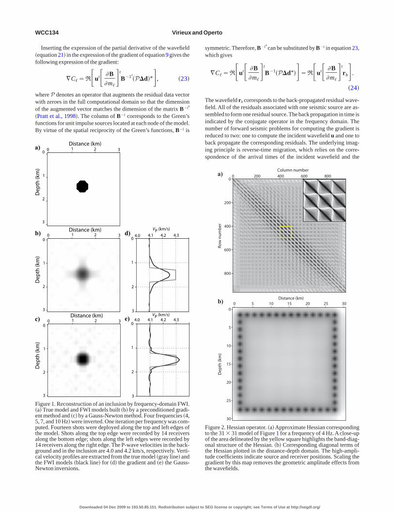
y the diagonal Hessian on one hand and the approximate Hessiann the other hand is provided in Figure 1. A single inclusion in a ho-ogeneous background model �Figure 1a� is reconstructed by one

teration of FWI using a gradient method preconditioned by the diag-nal terms of the approximate Hessian �Figure 1b� and by a Gauss-ewton method �Figure 1c�. The image of the inclusion is sharperhen the Gauss-Newton algorithm is used. The corresponding ap-roximate Hessian and its diagonal elements are shown in Figure 2.n interpretation of the second term of the Hessian �equation 10� isiven in Pratt et al. �1998�. This term accounts for multiscatteringvents such as multiples in the reconstruction procedure. Through it-rations, we might correct effects caused by this missing term asong as convergence is achieved.

Although equation 21 gives some clear insight into the physicalense of the gradient of the misfit function, it is impractical from aomputer-implementation point of view; with the computer explicit-y forming the sensitivity matrix with equation 21, it would requireerforming as many forward problems as the number of model pa-ameters m��1,M� for each source of the survey. To mitigate thisomputational burden, the spatial reciprocity of Green’s functionsan be exploited as shown below.


�f

wwo�fB

sw

Tfisinrbis

a

b

c

F�e5pta1gctN

Ftoottgt


Inserting the expression of the partial derivative of the wavefieldequation 21� in the expression of the gradient of equation 9 gives theollowing expression of the gradient:

�C��R�ut� �B

�m��t

B�1t�P�d�*�, �23�

here P denotes an operator that augments the residual data vectorith zeroes in the full computational domain so that the dimensionf the augmented vector matches the dimension of the matrix B�1t

Pratt et al., 1998�. The column of B�1 corresponds to the Green’sunctions for unit impulse sources located at each node of the model.y virtue of the spatial reciprocity of the Green’s functions, B�1 is

0 1 2 30

1

2

3

Distance (km)

Dep

th(k

m)

0 1 2 30

1

2

3

Dep

th(k

m)

0 1 2 30

1

2

3

Dep

th(k

m)

Distance (km)

Distance (km)4.0 4.1 4.2 4.3

0

1

2

3

4.0 4.1 4.2 4.30

1

2

3

VP (km/s)

VP (km/s)

)

)

)

d)

e)

igure 1. Reconstruction of an inclusion by frequency-domain FWI.a� True model and FWI models built �b� by a preconditioned gradi-nt method and �c� by a Gauss-Newton method. Four frequencies �4,, 7, and 10 Hz� were inverted. One iteration per frequency was com-uted. Fourteen shots were deployed along the top and left edges ofhe model. Shots along the top edge were recorded by 14 receiverslong the bottom edge; shots along the left edges were recorded by4 receivers along the right edge. The P-wave velocities in the back-round and in the inclusion are 4.0 and 4.2 km/s, respectively. Verti-al velocity profiles are extracted from the true model �gray line� andhe FWI models �black line� for �d� the gradient and �e� the Gauss-ewton inversions.


ymmetric. Therefore, B�1tcan be substituted by B�1 in equation 23,

hich gives

�C��R�ut� �B

�m��t

B�1�P�d*��R�ut� �B

�m��t

rb� .

�24�

he wavefield rb corresponds to the back-propagated residual wave-eld. All of the residuals associated with one seismic source are as-embled to form one residual source. The back propagation in time isndicated by the conjugate operator in the frequency domain. Theumber of forward seismic problems for computing the gradient iseduced to two: one to compute the incident wavefield u and one toack propagate the corresponding residuals. The underlying imag-ng principle is reverse-time migration, which relies on the corre-pondence of the arrival times of the incident wavefield and the

0

200

400

600

800

Rownu

mbe

rDep

th(km)

Column number0 200 400 600 800

0

5

10

15

20

25

30

Distance (km)0 5 10 15 20 25 30

a)

b)

igure 2. Hessian operator. �a� Approximate Hessian correspondingo the 31 � 31 model of Figure 1 for a frequency of 4 Hz.Aclose-upf the area delineated by the yellow square highlights the band-diag-nal structure of the Hessian. �b� Corresponding diagonal terms ofhe Hessian plotted in the distance-depth domain. The high-ampli-ude coefficients indicate source and receiver positions. Scaling theradient by this map removes the geometric amplitude effects fromhe wavefields.


bb

ffmmtagmTidjp

f

Wst1

2e

wotsdbsteidTvH�w

ptisfLaii

mont

aaepnvd1mrttfvfqf

S

abt�

wiFTomsh2

v2ooddsg

Re

fita


ack-propagated wavefield at the position of heterogeneity �Claer-out, 1971; Lailly, 1983; Tarantola, 1984�.The approach that consists of computing the gradient of the misfit

unction without explicitly building the sensitivity matrix is often re-erred to as the adjoint-wavefield approach by the geophysical com-unity. The underlying mathematical theory is the adjoint-stateethod of the optimization theory �Lions, 1972; Chavent, 1974�. In-

eresting links exist between optimization techniques used in FWInd assimilation methods, widely used in fluid mechanics �Tala-rand and Courtier, 1987�. A detailed review of the adjoint-stateethod with illustrations from several seismic problems is given inromp et al. �2005�, Askan �2006�, Plessix �2006�, and Epanomer-

takis et al. �2008�. The expression of the gradient of the frequency-omain FWI misfit function �equation 24� is derived from the ad-oint-state method and the method of the Lagrange multiplier in Ap-endix A.For multiple sources and multiple frequencies, the gradient is

ormed by the summation over these sources and frequencies:

�C�� i�1

N�

�s�1

Ns

R��Bi�1sst� �Bi

�m��t

�Bi�1�P�d

i,s* �� .

�25�

e also need to note that matrices Bi�1�i�1,N�� do not depend on

hots; therefore, any speedup toward resolving systems that involvehese matrices with multiple sources should be considered �Marfurt,984; Jo et al., 1996; Stekl and Pratt, 1998�.By comparing the expressions of the gradient in equations 9 and

4, we can conclude that one element of the sensitivity matrix is giv-n by

Jk�s,r�,��ust� �Bt

�m��B�1� r, �26�

here k�s,r� denotes a source-receiver couple of the acquisition ge-metry, with s and r denoting a shot and a receiver position, respec-ively. An impulse source � r is located at receiver position r. If theensitivity matrix must be built, one forward problem for the inci-ent wavefield and one forward problem per receiver position muste computed. Therefore, the number of simulations to build the sen-itivity matrix can be higher than that required by gradient estima-ion if the number of nonredundant receiver positions significantlyxceeds the number of nonredundant shots, or vice versa. Comput-ng each term of the sensitivity matrix is also required to compute theiagonal terms of the approximate Hessian Ha �Shin et al., 2001b�.o mitigate the resulting computational burden for coarse OBS sur-eys, Operto et al. �2006� suggest computing the diagonal terms ofa for a decimated shot acquisition. Alternatively, Shin et al.

2001a� propose using an approximation of the diagonal Hessian,hich can be computed at the same cost as the gradient.Although the matrix-free adjoint approach is widely used in ex-

loration seismology, the earthquake-seismology community tendso favor the scattering-integral method, which is based on the explic-t building of the sensitivity matrix �Chen et al., 2007�. The linearystem relating the model perturbation to the data perturbation isormed and solved with a conjugate-gradient algorithm such asSQR �Paige and Saunders, 1982a�. A comparative complexitynalysis of the adjoint approach and the scattering-integral approachs presented in Chen et al. �2007�, who conclude that the scattering-ntegral approach outperforms the adjoint approach for a regional to-


ographic problem. Indeed, the superiority of one approach over thether is highly dependent on the acquisition geometry �the relativeumber of sources and receivers� and the number of model parame-ers.

The formalism in equation 25 has been kept as general as possiblend can relate to the acoustic or the elastic wave equation. In thecoustic case, the wavefield is the pressure scalar wavefield; in thelastic case, the wavefield ideally is formed by the components of thearticle velocity and the pressure if the sensors have four compo-ents. Equation 25 can be translated in the time domain using Parse-al’s relation. The expression of the gradient in equation 25 can beeveloped equivalently using a functional analysis �Tarantola,984�. The partial derivatives of the wavefield with respect to theodel parameters are provided by the kernel of the Born integral that

elates the model perturbations to the wavefield perturbations. Mul-iplying the transpose of the resulting operator by the conjugate ofhe data residuals provides the expression of the gradient. The twoormalisms �matrix and functional� give the same expression, pro-ided the discretization of the partial differential operators are per-ormed consistently in the two approaches. The derivation in the fre-uency domain of the gradient of the misfit function using the twoormalisms is explicitly illustrated by Gelis et al. �2007�.

ource estimation

Source excitation is generally unknown and must be considereds an unknown of the problem �Pratt, 1999�. The source wavelet cane estimated by solving a linear inverse problem because the rela-ionship between the seismic wavefield and the source is linearequation 2�. The solution for the source is given by the expression

s��gcal�m0� dobs�

�gcal�m0� gcal�m0��, �27�

here gcal�m0� denotes the Green’s functions computed in the start-ng model m0. The source function can be estimated directly in theWI algorithm once the incident wavefields have been modeled.he source and the medium are updated alternatively over iterationsf the FWI. Note that it is possible to take advantage of source esti-ation to design alternative misfit functions based on the differential

emblance optimization �Pratt and Symes, 2002� or to define moreeuristic criteria to stop the iteration of the inversion �Jaiswal et al.,009�.Alternatively, new misfit functions have been designed so the in-

ersion becomes independent of the source function �Lee and Kim,003; Zhou and Greenhalgh, 2003�. The governing idea of the meth-d is to normalize each seismogram of a shot gather by the sum of allf the seismograms. This removes the dependency of the normalizedata with respect to the source and modifies the misfit function. Therawback is that this approach requires an explicit estimate of theensitivity matrix; the normalized residuals cannot be back propa-ated because they do not satisfy the wave equation.

SOME KEY FEATURES OF FWI

esolution power of FWI and relationship to thexperimental setup

The interpretation of the partial-derivative wavefield as the wave-eld scattered by the missing heterogeneities provides some connec-

ions between FWI and generalized diffraction tomography �Dev-ney and Zhang, 1991; Gelius et al., 1991�. Diffraction tomography


rWLiamat

wae

i�st

frt

w�Bdl

obdcgmmT

malwwti

hAsocss

tiusrlttwiPsm

pa6lctmflct

Fp�n

Fpeva


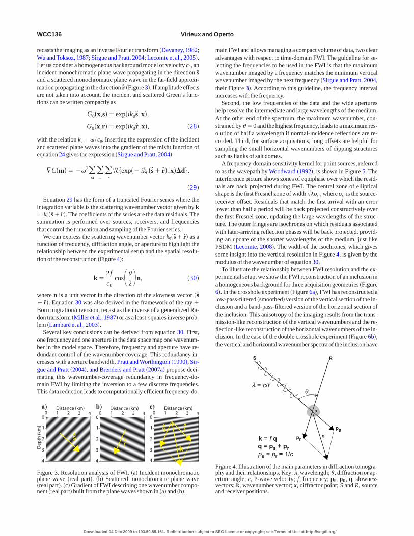
ecasts the imaging as an inverse Fourier transform �Devaney, 1982;u and Toksoz, 1987; Sirgue and Pratt, 2004; Lecomte et al., 2005�.

et us consider a homogeneous background model of velocity c0, anncident monochromatic plane wave propagating in the direction snd a scattered monochromatic plane wave in the far-field approxi-ation propagating in the direction r �Figure 3�. If amplitude effects

re not taken into account, the incident and scattered Green’s func-ions can be written compactly as

G0�x,s��exp�ik0s .x�,

G0�x,r��exp�ik0r .x�, �28�

ith the relation k0�� /c0. Inserting the expression of the incidentnd scattered plane waves into the gradient of the misfit function ofquation 24 gives the expression �Sirgue and Pratt, 2004�

�C�m��2��

�s

�r

R�exp�� ik0�s� r� .x��d� .

�29�

Equation 29 has the form of a truncated Fourier series where thentegration variable is the scattering wavenumber vector given by k

k0� s� r�. The coefficients of the series are the data residuals. Theummation is performed over sources, receivers, and frequencieshat control the truncation and sampling of the Fourier series.

We can express the scattering wavenumber vector k0� s� r� as aunction of frequency, diffraction angle, or aperture to highlight theelationship between the experimental setup and the spatial resolu-ion of the reconstruction �Figure 4�:

k�2f

c0cos�

2�n, �30�

here n is a unit vector in the direction of the slowness vector � sr�. Equation 30 was also derived in the framework of the ray

orn migration/inversion, recast as the inverse of a generalized Ra-on transform �Miller et al., 1987� or as a least-squares inverse prob-em �Lambaré et al., 2003�.

Several key conclusions can be derived from equation 30. First,ne frequency and one aperture in the data space map one wavenum-er in the model space. Therefore, frequency and aperture have re-undant control of the wavenumber coverage. This redundancy in-reases with aperture bandwidth. Pratt and Worthington �1990�, Sir-ue and Pratt �2004�, and Brenders and Pratt �2007a� propose deci-ating this wavenumber-coverage redundancy in frequency-do-ain FWI by limiting the inversion to a few discrete frequencies.his data reduction leads to computationally efficient frequency-do-

4

0

1

2

3

0 1 2 3 4Distance (km)

Dep

th(k

m)

0

1

2

3


0

1

2

3


4 4

sr k

s r

a) b) c)

igure 3. Resolution analysis of FWI. �a� Incident monochromaticlane wave �real part�. �b� Scattered monochromatic plane wavereal part�. �c� Gradient of FWI describing one wavenumber compo-ent �real part� built from the plane waves shown in �a� and �b�.


ain FWI and allows managing a compact volume of data, two cleardvantages with respect to time-domain FWI. The guideline for se-ecting the frequencies to be used in the FWI is that the maximumavenumber imaged by a frequency matches the minimum verticalavenumber imaged by the next frequency �Sirgue and Pratt, 2004,

heir Figure 3�. According to this guideline, the frequency intervalncreases with the frequency.

Second, the low frequencies of the data and the wide apertureselp resolve the intermediate and large wavelengths of the medium.t the other end of the spectrum, the maximum wavenumber, con-

trained by � 0 and the highest frequency, leads to a maximum res-lution of half a wavelength if normal-incidence reflections are re-orded. Third, for surface acquisitions, long offsets are helpful forampling the small horizontal wavenumbers of dipping structuresuch as flanks of salt domes.

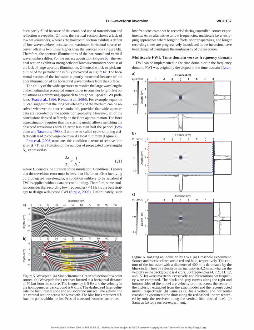
A frequency-domain sensitivity kernel for point sources, referredo as the wavepath by Woodward �1992�, is shown in Figure 5. Thenterference picture shows zones of equiphase over which the resid-als are back projected during FWI. The central zone of ellipticalhape is the first Fresnel zone of width ��osr, where osr is the source-eceiver offset. Residuals that match the first arrival with an errorower than half a period will be back projected constructively overhe first Fresnel zone, updating the large wavelengths of the struc-ure. The outer fringes are isochrones on which residuals associatedith later-arriving reflection phases will be back projected, provid-

ng an update of the shorter wavelengths of the medium, just likeSDM �Lecomte, 2008�. The width of the isochrones, which givesome insight into the vertical resolution in Figure 4, is given by theodulus of the wavenumber of equation 30.To illustrate the relationship between FWI resolution and the ex-

erimental setup, we show the FWI reconstruction of an inclusion inhomogeneous background for three acquisition geometries �Figure�. In the crosshole experiment �Figure 6a�, FWI has reconstructed aow-pass-filtered �smoothed� version of the vertical section of the in-lusion and a band-pass-filtered version of the horizontal section ofhe inclusion. This anisotropy of the imaging results from the trans-ission-like reconstruction of the vertical wavenumbers and the re-ection-like reconstruction of the horizontal wavenumbers of the in-lusion. In the case of the double crosshole experiment �Figure 6b�,he vertical and horizontal wavenumber spectra of the inclusion have

S R

pspr

x

q

θ

k = f q

λ = c/f

q = ps + prps = pr = 1/c

igure 4. Illustration of the main parameters in diffraction tomogra-hy and their relationships. Key: �, wavelength; , diffraction or ap-rture angle; c, P-wave velocity; f , frequency; pS, pR, q, slownessectors; k, wavenumber vector; x, diffractor point; S and R, sourcend receiver positions.


brlocTwttpzp

oql3sdcaodf

eN

wt5Fie

liprb

M

d

a

b

Fsoteif

V

a

b

c

FStbvacbtmceS


een partly filled because of the combined use of transmission andeflection wavepaths. Of note, the vertical section shows a lack ofow wavenumbers, whereas the horizontal section exhibits a deficitf low wavenumbers because the maximum horizontal source-re-eiver offset is two times higher than the vertical one �Figure 6b�.herefore, the aperture illuminations of the horizontal and verticalavenumbers differ. For the surface acquisition �Figure 6c�, the ver-

ical section exhibits a strong deficit of low wavenumbers because ofhe lack of large-aperture illumination. Of note, the pick-to-pick am-litude of the perturbation is fully recovered in Figure 6c. The hori-ontal section of the inclusion is poorly recovered because of theoor illumination of the horizontal wavenumbers from the surface.The ability of the wide apertures to resolve the large wavelengths

f the medium has prompted some studies to consider long-offset ac-uisitions as a promising approach to design well-posed FWI prob-ems �Pratt et al., 1996; Ravaut et al., 2004�. For example, equation0 can suggest that the long wavelengths of the medium can be re-olved whatever the source bandwidth, provided that wide-apertureata are recorded by the acquisition geometry. However, all of theonclusions derived so far rely on the Born approximation.The Bornpproximation requires that the starting model allows matching thebserved traveltimes with an error less than half the period �Bey-oun and Tarantola, 1988�. If not, the so-called cycle-skipping arti-acts will lead to convergence toward a local minimum �Figure 7�.

Pratt et al. �2008� translates this condition in terms of relative timerror �t /TL as a function of the number of propagated wavelengths�, expressed as

�t

TL�

1

N�

, �31�

here TL denotes the duration of the simulation. Condition 31 showshat the traveltime error must be less than 1% for an offset involving0 propagated wavelengths, a condition unlikely to be satisfied ifWI is applied without data preconditioning. Therefore, some stud-

es consider that recording low frequencies ��1 Hz� is the best strat-gy to design well-posed FWI �Sirgue, 2006�. Unfortunately, such

X

X

Xθ

0 10 20 30 40 50 60 70 80 90 100

0

5

10

15

20

Distance (km)0 10 20 30 40 50 60 70 80 90 100

0

5

10

15

20

Dep

th(k

m)

Dep

th(k

m)

s r

)

)

igure 5. Wavepath. �a� Monochromatic Green’s function for a pointource. �b� Wavepath for a receiver located at a horizontal distancef 70 km from the source. The frequency is 5 Hz and the velocity inhe homogeneous background is 6 km/s. The dashed red lines delin-ate the first Fresnel zone and an isochrone surface. The yellow lines a vertical section across the wavepath.The blue lines represent dif-raction paths within the first Fresnel zone and from the isochrone.


ow frequencies cannot be recorded during controlled-source exper-ments. As an alternative to low frequencies, multiscale layer-strip-ing approaches where longer offsets, shorter apertures, and longerecording times are progressively introduced in the inversion, haveeen designed to mitigate the nonlinearity of the inversion.

ultiscale FWI: Time domain versus frequency domainFWI can be implemented in the time domain or in the frequency

omain. FWI was originally developed in the time domain �Taran-

Dep

th(km)

Distance (km)0 1 2 3 4 5 6 7 8

0

1

2

3

4

(km/s)P

4.1

4.0

Distance (km)0 1 2 3 4 5 6 7 8

0

1

2

3

4

4.2

4.1

4.0

VP (km/s)

Distance (km)0 1 2 3 4 5 6 7 8

0

1

2

3

4

Dep

th(km)

4.0

3.9

VP (km/s)Distance (km)

0 1 2 3 4 5 6 7 80

1

2

3

4

Dep

th(km)

)

)

)

igure 6. Imaging an inclusion by FWI. �a� Crosshole experiment.ource and receiver lines are in red and blue, respectively. The con-

our of the inclusion with a diameter of 400 m is delineated by thelue circle. The true velocity in the inclusion is 4.2 km/s, whereas theelocity in the background is 4 km/s. Six frequencies �4, 7, 9, 11, 12,nd 15 Hz� were inverted successively, and 20 iterations per frequen-y were computed. The black and gray curves along the right andottom sides of the model are velocity profiles across the center ofhe inclusion extracted from the exact model and the reconstructedodel, respectively. �b� Same as �a� for a vertical and horizontal

rosshole experiment �the shots along the red dashed line are record-d by only the receivers along the vertical blue dashed line�. �c�ame as �a� for a surface experiment.


twttcs

sAtsrdwBisaidi

fitnewqqgomciow

iFtdldtwhrldlmcpte

ftbfvoB

wi

itoR

de�dotdogootttl

aaafl

FbfmttsFc


ola, 1984; Gauthier et al., 1986; Mora, 1987; Crase et al., 1990�hereas the frequency-domain approach was proposed mainly in

he 1990s by Pratt and collaborators �Pratt, 1990; Pratt and Wor-hington, 1990; Pratt and Goulty, 1991�, first with application torosshole data and later with application to wide-aperture surfaceeismic data �Pratt et al., 1996�.

The nonlinearity of FWI has prompted many studies to developome hierarchical multiscale strategies to mitigate this nonlinearity.part from computational efficiency, the flexibility offered by the

ime domain or the frequency domain to implement efficient multi-cale strategies is one of the main criteria that favors one domainather than the other. The multiscale strategy successively processesata subsets of increasing resolution power to incorporate smalleravenumbers in the tomographic models. In the time domain,unks et al. �1995� propose successive inversion of subdata sets of

ncreasing high-frequency content because low frequencies are lessensitive to cycle-skipping artifacts.The frequency domain providesmore natural framework for this multiscale approach by perform-

ng successive inversions of increasing frequencies. In the frequencyomain, single or multiple frequencies �i.e., frequency group� can benverted at a time.

Although a few discrete frequencies theoretically are sufficient toll the wavenumber spectrum for wide-aperture acquisitions, simul-

aneous inversion of multiple frequencies improves the signal-to-oise ratio and the robustness of FWI when complex wave phenom-na are observed �i.e., guide waves, surface waves, dispersiveaves�. Therefore, a trade-off between computational efficiency anduality of imaging must be found. When simultaneous multifre-uency inversion is performed, the bandwidth of the frequencyroup ideally must be as large as possible to mitigate the nonlinearityf FWI in terms of the nonunicity of the solution, whereas the maxi-um frequency of the group must be sufficiently low to prevent cy-

le-skipping artifacts. An illustration of this tuning of FWI is givenn Brossier et al. �2009a� in the framework of elastic seismic imagingf complex onshore models from the joint inversion of surfaceaves and body waves.

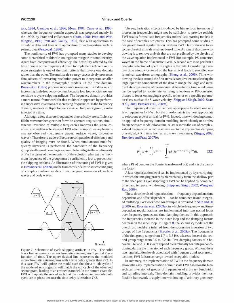
n n + 1n – 1

n

Time (s)

n + 1nn – 1

T/2 T/2

n + 1n – 1

igure 7. Schematic of cycle-skipping artifacts in FWI. The solidlack line represents a monochromatic seismogram of period T as aunction of time. The upper dashed line represents the modeledonochromatic seismograms with a time delay greater than T /2. In

his case, FWI will update the model such that the n�1th cycle ofhe modeled seismograms will match the nth cycle of the observedeismogram, leading to an erroneous model. In the bottom example,WI will update the model such that the modeled and recorded nthycle are in-phase because the time delay is less than T /2.


The regularization effects introduced by hierarchical inversion ofncreasing frequencies might not be sufficient to provide reliableWI results for realistic frequencies and realistic starting models in

he case of complex structures. This has prompted some studies toesign additional regularization levels in FWI. One of these is to se-ect a subset of arrivals as a function of time.An aim of this time win-owing is to remove arrivals that are not predicted by the physics ofhe wave equation implemented in FWI �for example, PS-convertedaves in the frame of acoustic FWI�. A second aim is to perform aeuristic selection of aperture angles in the data. Considering a nar-ow time window centered on the first arrival leads to so-called ear-y-arrival waveform tomography �Sheng et al., 2006�. Time win-owing the data around the first arrivals is equivalent to selecting thearge-aperture components of the data to image the large and inter-ediate wavelengths of the medium.Alternatively, time windowing

an be applied to isolate later-arriving reflections or PS-convertedhases to focus on imaging a specific reflector or a specific parame-er class, such as the S-wave velocity �Shipp and Singh, 2002; Searst al., 2008; Brossier et al., 2009a�.

The frequency domain is the most appropriate to select one or aew frequencies for FWI, but the time domain is the most appropriateo select one type of arrival for FWI. Indeed, time windowing cannote applied in frequency-domain modeling, in which only one or fewrequencies are modeled at a time.Alast resort is the use of complex-alued frequencies, which is equivalent to the exponential dampingf a signal p�t� in time from an arbitrary traveltime t0 �Sirgue, 2003;renders and Pratt, 2007b�:

P�� i

��et0/� ��

�

�

p�t�e��t�t0�/�ei�tdt, �32�

here P�� denotes the Fourier transform of p�t� and � is the damp-ng factor.

A last regularization level can be implemented by layer stripping,n which the imaging proceeds hierarchically from the shallow parto the deep part. Layer stripping in FWI can be applied by combinedffset and temporal windowing �Shipp and Singh, 2002; Wang andao, 2009�.These three levels of regularization — frequency dependent, time

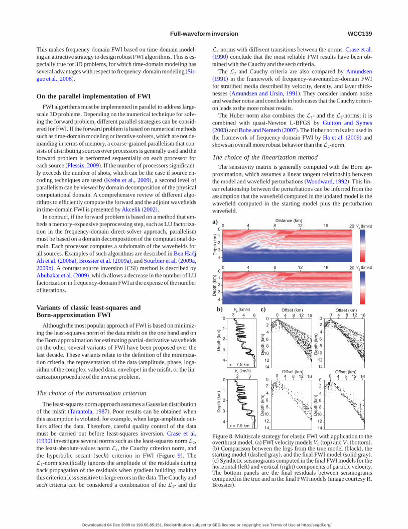
ependent, and offset dependent — can be combined in one integrat-d multiloop FWI workflow.An example is provided in Shin and Ha2009� and Brossier et al. �2009a�, in which the frequency- and time-ependent regularizations are implemented into two nested loopsver frequency groups and time-damping factors. In this approach,he frequencies increase in the outer loop and the damping factorsecrease in the inner loop. In Figure 8, the VP and VS models of theverthrust model are inferred from the successive inversion of tworoups of five frequencies �Brossier et al., 2009a�. The frequenciesf the first group range from 1.7 to 3.5 Hz, whereas those of the sec-nd group range from 3.5 to 7.2 Hz. Five damping factors of � be-ween 0.67 and 30.0 s were applied hierarchically for data precondi-ioning during the inversion of each frequency group. Without thesewo regularization levels associated with frequency and aperture se-ections, FWI fails to converge toward acceptable models.

In summary, the implementation of FWI in the frequency domainllows the easy implementation of multiscale FWI based on the hier-rchical inversion of groups of frequencies of arbitrary bandwidthnd sampling intervals. Time-domain modeling provides the mostexible framework to apply time windowing of arbitrary geometry.


Tipsg

O

siesmsfelcpcri

btmmaA2Afo

VB

itoltre

T

otlm�ttLbts

L�t

�fnao

c�ts

T

pteaww

Fo�s�hTcB


his makes frequency-domain FWI based on time-domain model-ng an attractive strategy to design robust FWI algorithms. This is es-ecially true for 3D problems, for which time-domain modeling haseveral advantages with respect to frequency-domain modeling �Sir-ue et al., 2008�.

n the parallel implementation of FWI

FWI algorithms must be implemented in parallel to address large-cale 3D problems. Depending on the numerical technique for solv-ng the forward problem, different parallel strategies can be consid-red for FWI. If the forward problem is based on numerical methodsuch as time-domain modeling or iterative solvers, which are not de-anding in terms of memory, a coarse-grained parallelism that con-

ists of distributing sources over processors is generally used and theorward problem is performed sequentially on each processor forach source �Plessix, 2009�. If the number of processors significant-y exceeds the number of shots, which can be the case if source en-oding techniques are used �Krebs et al., 2009�, a second level ofarallelism can be viewed by domain decomposition of the physicalomputational domain. A comprehensive review of different algo-ithms to efficiently compute the forward and the adjoint wavefieldsn time-domain FWI is presented by Akcelik �2002�.

In contract, if the forward problem is based on a method that em-eds a memory-expensive preprocessing step, such as LU factoriza-ion in the frequency-domain direct-solver approach, parallelismust be based on a domain decomposition of the computational do-ain. Each processor computes a subdomain of the wavefields for

ll sources. Examples of such algorithms are described in Ben Hadjli et al. �2008a�, Brossier et al. �2009a�, and Sourbier et al. �2009a,009b�. A contrast source inversion �CSI� method is described bybubakar et al. �2009�, which allows a decrease in the number of LU

actorization in frequency-domain FWI at the expense of the numberf iterations.

ariants of classic least-squares andorn-approximation FWI

Although the most popular approach of FWI is based on minimiz-ng the least-squares norm of the data misfit on the one hand and onhe Born approximation for estimating partial-derivative wavefieldsn the other, several variants of FWI have been proposed over theast decade. These variants relate to the definition of the minimiza-ion criteria, the representation of the data �amplitude, phase, loga-ithm of the complex-valued data, envelope� in the misfit, or the lin-arization procedure of the inverse problem.

he choice of the minimization criterion

The least-squares norm approach assumes a Gaussian distributionf the misfit �Tarantola, 1987�. Poor results can be obtained whenhis assumption is violated, for example, when large-amplitude out-iers affect the data. Therefore, careful quality control of the dataust be carried out before least-squares inversion. Crase et al.

1990� investigate several norms such as the least-squares norm L2,he least-absolute-values norm L1, the Cauchy criterion norm, andhe hyperbolic secant �sech� criterion in FWI �Figure 9�. The

1-norm specifically ignores the amplitude of the residuals duringack propagation of the residuals when gradient building, makinghis criterion less sensitive to large errors in the data.The Cauchy andech criteria can be considered a combination of the L - and the
1

2-norms with different transitions between the norms. Crase et al.1990� conclude that the most reliable FWI results have been ob-ained with the Cauchy and the sech criteria.

The L2 and Cauchy criteria are also compared by Amundsen1991� in the framework of frequency-wavenumber-domain FWIor stratified media described by velocity, density, and layer thick-esses �Amundsen and Ursin, 1991�. They consider random noisend weather noise and conclude in both cases that the Cauchy criteri-n leads to the more robust results.The Huber norm also combines the L1- and the L2-norms; it is

ombined with quasi-Newton L-BFGS by Guitton and Symes2003� and Bube and Nemeth �2007�. The Huber norm is also used inhe framework of frequency-domain FWI by Ha et al. �2009� andhows an overall more robust behavior than the L2-norm.

he choice of the linearization method

The sensitivity matrix is generally computed with the Born ap-roximation, which assumes a linear tangent relationship betweenhe model and wavefield perturbations �Woodward, 1992�. This lin-ar relationship between the perturbations can be inferred from thessumption that the wavefield computed in the updated model is theavefield computed in the starting model plus the perturbationavefield.

VP

(km/s)

VS

(km/s)

0 4 8 12 16 20012

3

4

0 4 8 12 16 20012

3

4

0 4 8 12 1602

468

101214

Depth(km)

0 4 8 12 1602

468

101214

Depth(km)

0 4 8 12 1602

468

101214

Depth(km)

0 4 8 12 1602

468

101214

Depth(km)

Depth(km)

Depth(km)

0

1

2

3

4

Depth(km)

0

1

2

3

4

Depth(km)

3 4 6

2 3

Offset (km) Offset (km)

Offset (km) Offset (km)VS

(km/s)

VP

(km/s)

x = 7.5 km

x = 7.5 km

Distance (km)a)

b) c)

igure 8. Multiscale strategy for elastic FWI with application to theverthrust model. �a� FWI velocity models VP �top� and VS �bottom�.b� Comparison between the logs from the true model �black�, thetarting model �dashed gray�, and the final FWI model �solid gray�.c� Synthetic seismograms computed in the final FWI models for theorizontal �left� and vertical �right� components of particle velocity.he bottom panels are the final residuals between seismogramsomputed in the true and in the final FWI models �image courtesy R.rossier�.


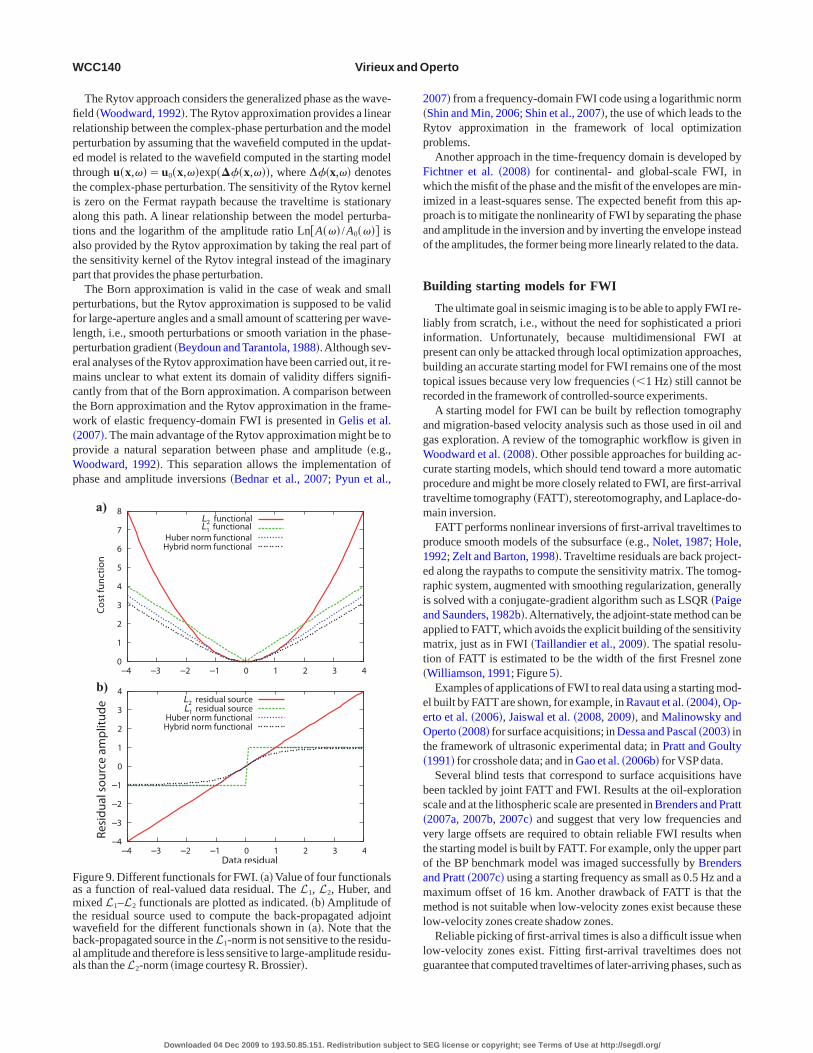
firpettiatatp

pflpemctw�pWp

2�Rp

Fwipao

B

lipbtr

agWcptm

p1eriaamt�

ee

toamml

lg

Famtwbaa


The Rytov approach considers the generalized phase as the wave-eld �Woodward, 1992�. The Rytov approximation provides a linearelationship between the complex-phase perturbation and the modelerturbation by assuming that the wavefield computed in the updat-d model is related to the wavefield computed in the starting modelhrough u�x,��u0�x,��exp��x,��, where ∆��x,�� denoteshe complex-phase perturbation. The sensitivity of the Rytov kernels zero on the Fermat raypath because the traveltime is stationarylong this path. A linear relationship between the model perturba-ions and the logarithm of the amplitude ratio Ln�A�� /A0�� islso provided by the Rytov approximation by taking the real part ofhe sensitivity kernel of the Rytov integral instead of the imaginaryart that provides the phase perturbation.The Born approximation is valid in the case of weak and small

erturbations, but the Rytov approximation is supposed to be validor large-aperture angles and a small amount of scattering per wave-ength, i.e., smooth perturbations or smooth variation in the phase-erturbation gradient �Beydoun and Tarantola, 1988�.Although sev-ral analyses of the Rytov approximation have been carried out, it re-ains unclear to what extent its domain of validity differs signifi-

antly from that of the Born approximation. A comparison betweenhe Born approximation and the Rytov approximation in the frame-ork of elastic frequency-domain FWI is presented in Gelis et al.

2007�. The main advantage of the Rytov approximation might be torovide a natural separation between phase and amplitude �e.g.,oodward, 1992�. This separation allows the implementation of

hase and amplitude inversions �Bednar et al., 2007; Pyun et al.,

0

1

2

3

4

5

6

7

8

–4 –3 –2 –1 0 1 2 3 4

L2 functionalL1 functional

Huber norm functionalHybrid norm functional

Co

stfu

nct

ion

–1

–2

–3

–4

0

1

2

3

4

–4 –3 –2 –1 0 1 2 3 4

Residu

alsource

amplitu

de

L2 residual sourceL1 residual source

Huber norm functionalHybrid norm functional

Data residual

a)

b)

igure 9. Different functionals for FWI. �a� Value of four functionalss a function of real-valued data residual. The L1, L2, Huber, andixed L1–L2 functionals are plotted as indicated. �b� Amplitude of

he residual source used to compute the back-propagated adjointavefield for the different functionals shown in �a�. Note that theack-propagated source in the L1-norm is not sensitive to the residu-l amplitude and therefore is less sensitive to large-amplitude residu-ls than the L -norm �image courtesy R. Brossier�.
2

007� from a frequency-domain FWI code using a logarithmic normShin and Min, 2006; Shin et al., 2007�, the use of which leads to theytov approximation in the framework of local optimizationroblems.Another approach in the time-frequency domain is developed by

ichtner et al. �2008� for continental- and global-scale FWI, inhich the misfit of the phase and the misfit of the envelopes are min-

mized in a least-squares sense. The expected benefit from this ap-roach is to mitigate the nonlinearity of FWI by separating the phasend amplitude in the inversion and by inverting the envelope insteadf the amplitudes, the former being more linearly related to the data.

uilding starting models for FWI

The ultimate goal in seismic imaging is to be able to apply FWI re-iably from scratch, i.e., without the need for sophisticated a priorinformation. Unfortunately, because multidimensional FWI atresent can only be attacked through local optimization approaches,uilding an accurate starting model for FWI remains one of the mostopical issues because very low frequencies ��1 Hz� still cannot beecorded in the framework of controlled-source experiments.

A starting model for FWI can be built by reflection tomographynd migration-based velocity analysis such as those used in oil andas exploration. A review of the tomographic workflow is given inoodward et al. �2008�. Other possible approaches for building ac-

urate starting models, which should tend toward a more automaticrocedure and might be more closely related to FWI, are first-arrivalraveltime tomography �FATT�, stereotomography, and Laplace-do-ain inversion.FATT performs nonlinear inversions of first-arrival traveltimes to

roduce smooth models of the subsurface �e.g., Nolet, 1987; Hole,992; Zelt and Barton, 1998�. Traveltime residuals are back project-d along the raypaths to compute the sensitivity matrix. The tomog-aphic system, augmented with smoothing regularization, generallys solved with a conjugate-gradient algorithm such as LSQR �Paigend Saunders, 1982b�.Alternatively, the adjoint-state method can bepplied to FATT, which avoids the explicit building of the sensitivityatrix, just as in FWI �Taillandier et al., 2009�. The spatial resolu-

ion of FATT is estimated to be the width of the first Fresnel zoneWilliamson, 1991; Figure 5�.

Examples of applications of FWI to real data using a starting mod-l built by FATT are shown, for example, in Ravaut et al. �2004�, Op-rto et al. �2006�, Jaiswal et al. �2008, 2009�, and Malinowsky and

Operto �2008� for surface acquisitions; in Dessa and Pascal �2003� inthe framework of ultrasonic experimental data; in Pratt and Goulty�1991� for crosshole data; and in Gao et al. �2006b� for VSPdata.

Several blind tests that correspond to surface acquisitions havebeen tackled by joint FATT and FWI. Results at the oil-explorationscale and at the lithospheric scale are presented in Brenders and Pratt�2007a, 2007b, 2007c� and suggest that very low frequencies andvery large offsets are required to obtain reliable FWI results whenhe starting model is built by FATT. For example, only the upper partf the BP benchmark model was imaged successfully by Brendersnd Pratt �2007c� using a starting frequency as small as 0.5 Hz and aaximum offset of 16 km. Another drawback of FATT is that theethod is not suitable when low-velocity zones exist because these

ow-velocity zones create shadow zones.Reliable picking of first-arrival times is also a difficult issue when

ow-velocity zones exist. Fitting first-arrival traveltimes does notuarantee that computed traveltimes of later-arriving phases, such as


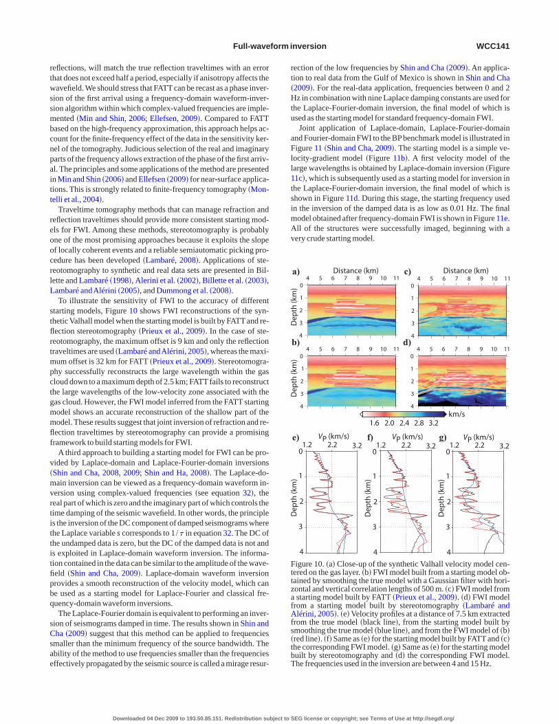
rtwssmbcnpaitt

reoocrlL

stflrtmpctgmmflf

v�mvrtittitfipbq

sCsae

rt�Htu

aFll1tsimAv

FttzafAfs�tbT


eflections, will match the true reflection traveltimes with an errorhat does not exceed half a period, especially if anisotropy affects theavefield. We should stress that FATT can be recast as a phase inver-

ion of the first arrival using a frequency-domain waveform-inver-ion algorithm within which complex-valued frequencies are imple-ented �Min and Shin, 2006; Ellefsen, 2009�. Compared to FATT

ased on the high-frequency approximation, this approach helps ac-ount for the finite-frequency effect of the data in the sensitivity ker-el of the tomography. Judicious selection of the real and imaginaryarts of the frequency allows extraction of the phase of the first arriv-l. The principles and some applications of the method are presentedn Min and Shin �2006� and Ellefsen �2009� for near-surface applica-ions. This is strongly related to finite-frequency tomography �Mon-elli et al., 2004�.

Traveltime tomography methods that can manage refraction andeflection traveltimes should provide more consistent starting mod-ls for FWI. Among these methods, stereotomography is probablyne of the most promising approaches because it exploits the slopef locally coherent events and a reliable semiautomatic picking pro-edure has been developed �Lambaré, 2008�. Applications of ste-eotomography to synthetic and real data sets are presented in Bil-ette and Lambaré �1998�, Alerini et al. �2002�, Billette et al. �2003�,ambaré andAlérini �2005�, and Dummong et al. �2008�.To illustrate the sensitivity of FWI to the accuracy of different

tarting models, Figure 10 shows FWI reconstructions of the syn-hetic Valhall model when the starting model is built by FATT and re-ection stereotomography �Prieux et al., 2009�. In the case of ste-eotomography, the maximum offset is 9 km and only the reflectionraveltimes are used �Lambaré andAlérini, 2005�, whereas the maxi-um offset is 32 km for FATT �Prieux et al., 2009�. Stereotomogra-

hy successfully reconstructs the large wavelength within the gasloud down to a maximum depth of 2.5 km; FATTfails to reconstructhe large wavelengths of the low-velocity zone associated with theas cloud. However, the FWI model inferred from the FATT startingodel shows an accurate reconstruction of the shallow part of theodel. These results suggest that joint inversion of refraction and re-ection traveltimes by stereotomography can provide a promisingramework to build starting models for FWI.

A third approach to building a starting model for FWI can be pro-ided by Laplace-domain and Laplace-Fourier-domain inversionsShin and Cha, 2008, 2009; Shin and Ha, 2008�. The Laplace-do-ain inversion can be viewed as a frequency-domain waveform in-

ersion using complex-valued frequencies �see equation 32�, theeal part of which is zero and the imaginary part of which controls theime damping of the seismic wavefield. In other words, the principles the inversion of the DC component of damped seismograms wherehe Laplace variable s corresponds to 1 /� in equation 32. The DC ofhe undamped data is zero, but the DC of the damped data is not ands exploited in Laplace-domain waveform inversion. The informa-ion contained in the data can be similar to the amplitude of the wave-eld �Shin and Cha, 2009�. Laplace-domain waveform inversionrovides a smooth reconstruction of the velocity model, which cane used as a starting model for Laplace-Fourier and classical fre-uency-domain waveform inversions.The Laplace-Fourier domain is equivalent to performing an inver-

ion of seismograms damped in time. The results shown in Shin andha �2009� suggest that this method can be applied to frequenciesmaller than the minimum frequency of the source bandwidth. Thebility of the method to use frequencies smaller than the frequenciesffectively propagated by the seismic source is called a mirage resur-


ection of the low frequencies by Shin and Cha �2009�. An applica-ion to real data from the Gulf of Mexico is shown in Shin and Cha2009�. For the real-data application, frequencies between 0 and 2z in combination with nine Laplace damping constants are used for

he Laplace-Fourier-domain inversion, the final model of which issed as the starting model for standard frequency-domain FWI.Joint application of Laplace-domain, Laplace-Fourier-domain

nd Fourier-domain FWI to the BPbenchmark model is illustrated inigure 11 �Shin and Cha, 2009�. The starting model is a simple ve-

ocity-gradient model �Figure 11b�. A first velocity model of thearge wavelengths is obtained by Laplace-domain inversion �Figure1c�, which is subsequently used as a starting model for inversion inhe Laplace-Fourier-domain inversion, the final model of which ishown in Figure 11d. During this stage, the starting frequency usedn the inversion of the damped data is as low as 0.01 Hz. The finalodel obtained after frequency-domain FWI is shown in Figure 11e.ll of the structures were successfully imaged, beginning with aery crude starting model.

4

3

2

1

04 5 6 7 8 9 10 11

4

3

2

1

04 5 6 7 8 9 10 11

Dep

th(k

m)

Distance (km) Distance (km)

4

3

2

1

04 5 6 7 8 9 10 11

4

3

2

1

04 5 6 7 8 9 10 11

Dep

th(k

m)

1.6 2.0 2.4 2.8 3.2km/s

1.2 2.2 3.20

1

2

3

4

Dep

th(k

m)

VP (km/s)1.2 2.2 3.2

0

1

2

3

4

Dep

th(k

m)

VP (km/s)1.2 2.2 3.2

0

1

2

3

4

Dep

th(k

m)

VP (km/s)

a)

b)

c)

d)

e) f) g)

igure 10. �a� Close-up of the synthetic Valhall velocity model cen-ered on the gas layer. �b� FWI model built from a starting model ob-ained by smoothing the true model with a Gaussian filter with hori-ontal and vertical correlation lengths of 500 m. �c� FWI model fromstarting model built by FATT �Prieux et al., 2009�. �d� FWI model

rom a starting model built by stereotomography �Lambaré andlérini, 2005�. �e� Velocity profiles at a distance of 7.5 km extracted

rom the true model �black line�, from the starting model built bymoothing the true model �blue line�, and from the FWI model of �b�red line�. �f� Same as �e� for the starting model built by FATT and �c�he corresponding FWI model. �g� Same as �e� for the starting modeluilt by stereotomography and �d� the corresponding FWI model.he frequencies used in the inversion are between 4 and 15 Hz.


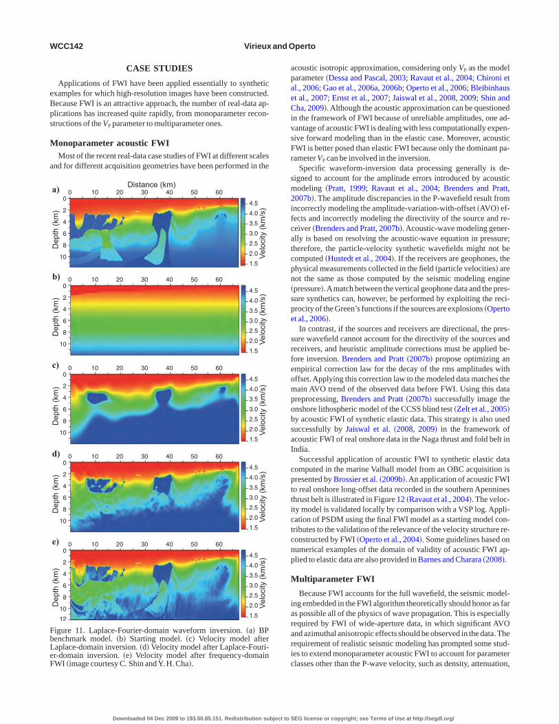
eBps

M

a

apaeCivsFr

sm2ifcatcpn�spe

srfeompobsaI

cpttictcnp

M

iararic

FbLeF


CASE STUDIES

Applications of FWI have been applied essentially to syntheticxamples for which high-resolution images have been constructed.ecause FWI is an attractive approach, the number of real-data ap-lications has increased quite rapidly, from monoparameter recon-tructions of the VP parameter to multiparameter ones.

onoparameter acoustic FWIMost of the recent real-data case studies of FWI at different scales

nd for different acquisition geometries have been performed in the

Distance (km)

Depth(km)

Depth(km)

Depth(km)

Depth(km)

Depth(km)

Velocity(km/s)

Velocity(km/s)

Velocity(km/s)

Velocity(km/s)

Velocity(km/s)

0 10 20 30 40 50 600

4.52 4.04 3.5

6 3.0

2.582.0101.5

0 10 20 30 40 50 600

4.52 4.04 3.5

6 3.0

2.582.0101.5

0 10 20 30 40 50 600

4.52 4.04 3.5

6 3.0

2.582.0101.5

0 10 20 30 40 50 600

4.52 4.04 3.5

6 3.0

2.582.0101.5

0 10 20 30 40 50 600

4.52 4.04 3.5

6 3.0

2.582.0101.512

a)

b)

c)

d)

e)

igure 11. Laplace-Fourier-domain waveform inversion. �a� BPenchmark model. �b� Starting model. �c� Velocity model afteraplace-domain inversion. �d� Velocity model after Laplace-Fouri-r-domain inversion. �e� Velocity model after frequency-domainWI �image courtesy C. Shin andY. H. Cha�.


coustic isotropic approximation, considering only VP as the modelarameter �Dessa and Pascal, 2003; Ravaut et al., 2004; Chironi etl., 2006; Gao et al., 2006a, 2006b; Operto et al., 2006; Bleibinhaust al., 2007; Ernst et al., 2007; Jaiswal et al., 2008, 2009; Shin andha, 2009�.Although the acoustic approximation can be questioned

n the framework of FWI because of unreliable amplitudes, one ad-antage of acoustic FWI is dealing with less computationally expen-ive forward modeling than in the elastic case. Moreover, acousticWI is better posed than elastic FWI because only the dominant pa-ameter VP can be involved in the inversion.

Specific waveform-inversion data processing generally is de-igned to account for the amplitude errors introduced by acousticodeling �Pratt, 1999; Ravaut et al., 2004; Brenders and Pratt,

007b�. The amplitude discrepancies in the P-wavefield result fromncorrectly modeling the amplitude-variation-with-offset �AVO� ef-ects and incorrectly modeling the directivity of the source and re-eiver �Brenders and Pratt, 2007b�. Acoustic-wave modeling gener-lly is based on resolving the acoustic-wave equation in pressure;herefore, the particle-velocity synthetic wavefields might not beomputed �Hustedt et al., 2004�. If the receivers are geophones, thehysical measurements collected in the field �particle velocities� areot the same as those computed by the seismic modeling enginepressure�.Amatch between the vertical geophone data and the pres-ure synthetics can, however, be performed by exploiting the reci-rocity of the Green’s functions if the sources are explosions �Opertot al., 2006�.

In contrast, if the sources and receivers are directional, the pres-ure wavefield cannot account for the directivity of the sources andeceivers, and heuristic amplitude corrections must be applied be-ore inversion. Brenders and Pratt �2007b� propose optimizing anmpirical correction law for the decay of the rms amplitudes withffset.Applying this correction law to the modeled data matches theain AVO trend of the observed data before FWI. Using this data

reprocessing, Brenders and Pratt �2007b� successfully image thenshore lithospheric model of the CCSS blind test �Zelt et al., 2005�y acoustic FWI of synthetic elastic data. This strategy is also useduccessfully by Jaiswal et al. �2008, 2009� in the framework ofcoustic FWI of real onshore data in the Naga thrust and fold belt inndia.

Successful application of acoustic FWI to synthetic elastic dataomputed in the marine Valhall model from an OBC acquisition isresented by Brossier et al. �2009b�.An application of acoustic FWIo real onshore long-offset data recorded in the southern Apennineshrust belt is illustrated in Figure 12 �Ravaut et al., 2004�. The veloc-ty model is validated locally by comparison with a VSP log. Appli-ation of PSDM using the final FWI model as a starting model con-ributes to the validation of the relevance of the velocity structure re-onstructed by FWI �Operto et al., 2004�. Some guidelines based onumerical examples of the domain of validity of acoustic FWI ap-lied to elastic data are also provided in Barnes and Charara �2008�.

ultiparameter FWI

Because FWI accounts for the full wavefield, the seismic model-ng embedded in the FWI algorithm theoretically should honor as fars possible all of the physics of wave propagation. This is especiallyequired by FWI of wide-aperture data, in which significant AVOnd azimuthal anisotropic effects should be observed in the data.Theequirement of realistic seismic modeling has prompted some stud-es to extend monoparameter acoustic FWI to account for parameterlasses other than the P-wave velocity, such as density, attenuation,


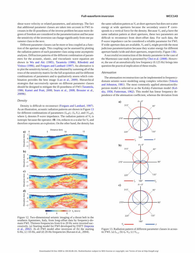
stcgtr

ttaesVtrcbss12

D

Afwit

tessdPIja

teq

A

dapsp

Fsmce6

Ft


hear-wave velocity or related parameters, and anisotropy. The facthat additional parameter classes are taken into account in FWI in-reases in the ill-posedness of the inverse problem because more de-rees of freedom are considered in the parameterization and becausehe sensitivity of the inversion can change significantly from one pa-ameter class to the next.

Different parameter classes can be more or less coupled as a func-ion of the aperture angle. This coupling can be assessed by plottinghe radiation pattern of each parameter class using some asymptoticnalyses. Diffraction patterns of the different combination of param-ters for the acoustic, elastic, and viscoelastic wave equation arehown in Wu and Aki �1985�, Tarantola �1986�, Ribodetti andirieux �1996�, and Forgues and Lambaré �1997�. An alternative is

o plot the sensitivity kernel, i.e., that obtained by summing all of theows of the sensitivity matrix for the full acquisition and for differentombinations of parameters and to qualitatively assess which com-ination provides the best image �Luo et al., 2009�. Hierarchicaltrategies that successively operate on different parameter classeshould be designed to mitigate the ill-posedness of FWI �Tarantola,986; Kamei and Pratt, 2008; Sears et al., 2008; Brossier et al.,009b�.

ensity

Density is difficult to reconstruct �Forgues and Lambaré, 1997�.s an illustration, acoustic radiation patterns are shown in Figure 13

or different combinations of parameters �IP,��, �IP,VP�, and �VP,��,here IP denotes P-wave impedance. The radiation pattern of VP is

sotropic because the operator �B /�ml reduces to a scalar for VP andherefore represents an explosion. On the other hand, the density has

2 4 6VP (km/s)

1

0

–1

–2Elev

atio

n(k

m)

1

0

–1

–2Elev

atio

n(k

m)

1

0

–1

–2Elev

atio

n(k

m)

1

0

–1

–2

0 5 10 15

Elev

atio

n(k

m)

Distance (km)a)

b)

c)

d)

igure 12. Two-dimensional seismic imaging of a thrust belt in theouthern Apennines, Italy, from long-offset data by frequency-do-ain FWI. Thirteen frequencies from 6 to 20 Hz were inverted suc-

essively. �a� Starting model for FWI developed by FATT �Improtat al., 2002�. �b–d� FWI model after inversion of �b� the starting-Hz, �c� 10-Hz, and �d� 20-Hz frequencies �Ravaut et al., 2004�.


he same radiation pattern as VP at short apertures but does not scatternergy at wide apertures because the secondary source f� corre-ponds to a vertical force for the density. Because VP and � have theame radiation pattern at short apertures, these two parameters areifficult to reconstruct from short-offset data. For such data, the-wave impedance can be considered a reliable parameter for FWI.f wide-aperture data are available, VP and IP might provide the mostudicious parameterization because they scatter energy for differentperture bands �wide and short apertures, respectively; Figure 13b�.

Asuccessful reconstruction of the density parameter in the case ofhe Marmousi case study is presented by Choi et al. �2008�. Howev-r, the use of an unrealistically low frequency �0.125 Hz� brings intouestion the practical implication of these results.

ttenuation

The attenuation reconstruction can be implemented in frequency-omain seismic-wave modeling using complex velocities �Toksöznd Johnston, 1981�. The most commonly applied attenuation/dis-ersion model is referred to as the Kolsky-Futterman model �Kol-ky, 1956; Futterman, 1962�. This model has linear frequency de-endence of the attenuation coefficient, whereas the deviation from

45°

90°

135°

180°

225°

270°

315°

45°

90°

135°

180°

225°

270°

315°

θ = 0°

45°

90°

135°

180°

225°

270°

315°

ρ

ρ

θ = 0°

θ = 0°

IP

VP

IP V

P

a)

b)

c)

igure 13. Radiation pattern of different parameter classes in acous-ic FWI. �a� I ; �b� I -V ; �c� V .
P-� P P P-�

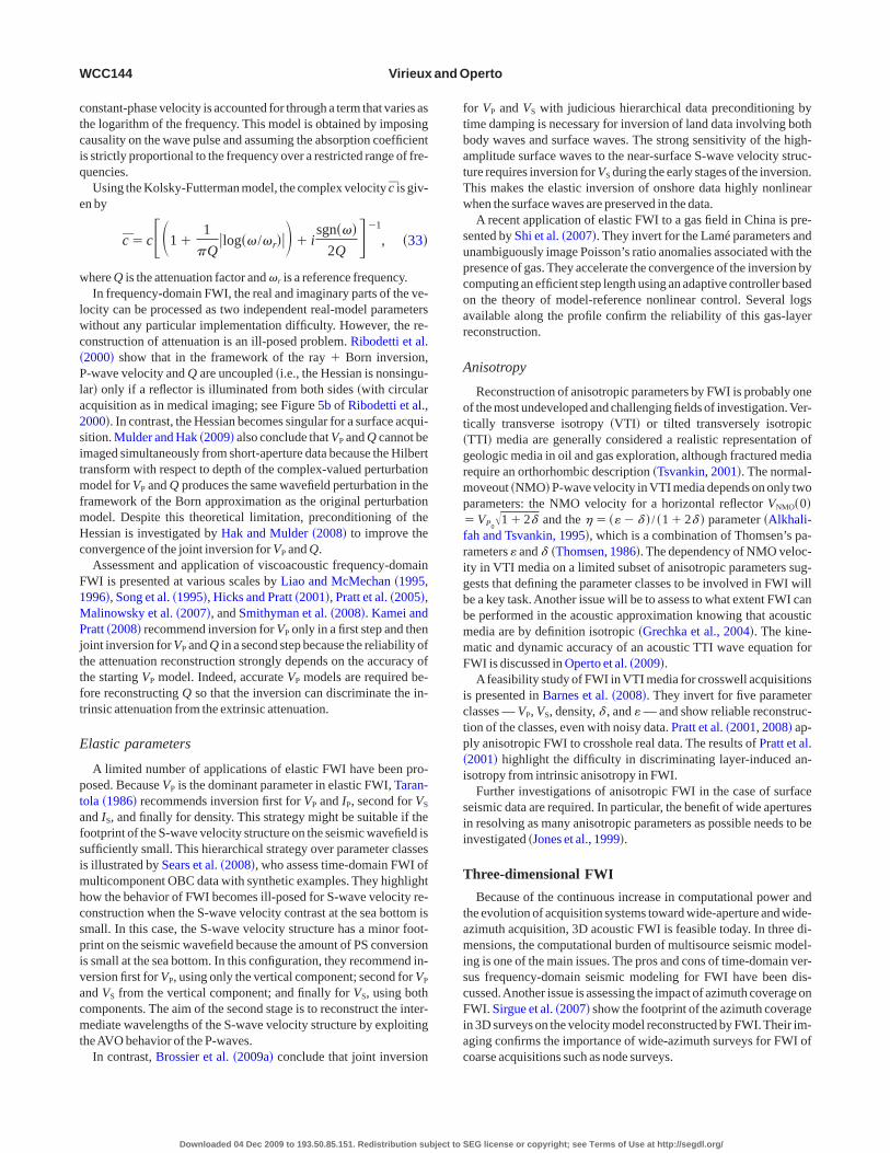
ctciq

e

w

lwc�Pla2sitmfmHc

F1MPjttft

E

ptafsimhcspivacmt

ftbatTw

supcoar

A

ot�grmp�frigbbmmF

ictp�i

sii

T

tamiscFiac


onstant-phase velocity is accounted for through a term that varies ashe logarithm of the frequency. This model is obtained by imposingausality on the wave pulse and assuming the absorption coefficients strictly proportional to the frequency over a restricted range of fre-uencies.Using the Kolsky-Futterman model, the complex velocity c is giv-

n by

c�c��1�1

�Q log�� /�r� �� i

sgn��2Q

��1

, �33�

here Q is the attenuation factor and �r is a reference frequency.In frequency-domain FWI, the real and imaginary parts of the ve-

ocity can be processed as two independent real-model parametersithout any particular implementation difficulty. However, the re-

onstruction of attenuation is an ill-posed problem. Ribodetti et al.2000� show that in the framework of the ray Born inversion,-wave velocity and Q are uncoupled �i.e., the Hessian is nonsingu-

ar� only if a reflector is illuminated from both sides �with circularcquisition as in medical imaging; see Figure 5b of Ribodetti et al.,000�. In contrast, the Hessian becomes singular for a surface acqui-ition. Mulder and Hak �2009� also conclude that VP and Q cannot bemaged simultaneously from short-aperture data because the Hilbertransform with respect to depth of the complex-valued perturbationodel for VP and Q produces the same wavefield perturbation in the

ramework of the Born approximation as the original perturbationodel. Despite this theoretical limitation, preconditioning of theessian is investigated by Hak and Mulder �2008� to improve the

onvergence of the joint inversion for VP and Q.Assessment and application of viscoacoustic frequency-domain

WI is presented at various scales by Liao and McMechan �1995,996�, Song et al. �1995�, Hicks and Pratt �2001�, Pratt et al. �2005�,alinowsky et al. �2007�, and Smithyman et al. �2008�. Kamei and

ratt �2008� recommend inversion for VP only in a first step and thenoint inversion for VP and Q in a second step because the reliability ofhe attenuation reconstruction strongly depends on the accuracy ofhe starting VP model. Indeed, accurate VP models are required be-ore reconstructing Q so that the inversion can discriminate the in-rinsic attenuation from the extrinsic attenuation.

lastic parameters

A limited number of applications of elastic FWI have been pro-osed. Because VP is the dominant parameter in elastic FWI, Taran-ola �1986� recommends inversion first for VP and IP, second for VS

nd IS, and finally for density. This strategy might be suitable if theootprint of the S-wave velocity structure on the seismic wavefield isufficiently small. This hierarchical strategy over parameter classess illustrated by Sears et al. �2008�, who assess time-domain FWI ofulticomponent OBC data with synthetic examples. They highlight

ow the behavior of FWI becomes ill-posed for S-wave velocity re-onstruction when the S-wave velocity contrast at the sea bottom ismall. In this case, the S-wave velocity structure has a minor foot-rint on the seismic wavefield because the amount of PS conversions small at the sea bottom. In this configuration, they recommend in-ersion first for VP, using only the vertical component; second for VP

nd VS from the vertical component; and finally for VS, using bothomponents. The aim of the second stage is to reconstruct the inter-ediate wavelengths of the S-wave velocity structure by exploiting

heAVO behavior of the P-waves.In contrast, Brossier et al. �2009a� conclude that joint inversion


or VP and VS with judicious hierarchical data preconditioning byime damping is necessary for inversion of land data involving bothody waves and surface waves. The strong sensitivity of the high-mplitude surface waves to the near-surface S-wave velocity struc-ure requires inversion for VS during the early stages of the inversion.his makes the elastic inversion of onshore data highly nonlinearhen the surface waves are preserved in the data.A recent application of elastic FWI to a gas field in China is pre-

ented by Shi et al. �2007�. They invert for the Lamé parameters andnambiguously image Poisson’s ratio anomalies associated with theresence of gas. They accelerate the convergence of the inversion byomputing an efficient step length using an adaptive controller basedn the theory of model-reference nonlinear control. Several logsvailable along the profile confirm the reliability of this gas-layereconstruction.

nisotropy

Reconstruction of anisotropic parameters by FWI is probably onef the most undeveloped and challenging fields of investigation.Ver-ically transverse isotropy �VTI� or tilted transversely isotropicTTI� media are generally considered a realistic representation ofeologic media in oil and gas exploration, although fractured mediaequire an orthorhombic description �Tsvankin, 2001�. The normal-oveout �NMO� P-wave velocity inVTI media depends on only twoarameters: the NMO velocity for a horizontal reflector VNMO�0�

VP0�1�2� and the � � �� / �1�2� � parameter �Alkhali-

ah and Tsvankin, 1995�, which is a combination of Thomsen’s pa-ameters � and � �Thomsen, 1986�. The dependency of NMO veloc-ty in VTI media on a limited subset of anisotropic parameters sug-ests that defining the parameter classes to be involved in FWI wille a key task.Another issue will be to assess to what extent FWI cane performed in the acoustic approximation knowing that acousticedia are by definition isotropic �Grechka et al., 2004�. The kine-atic and dynamic accuracy of an acoustic TTI wave equation forWI is discussed in Operto et al. �2009�.Afeasibility study of FWI in VTI media for crosswell acquisitions

s presented in Barnes et al. �2008�. They invert for five parameterlasses — VP, VS, density, � , and � — and show reliable reconstruc-ion of the classes, even with noisy data. Pratt et al. �2001, 2008� ap-ly anisotropic FWI to crosshole real data. The results of Pratt et al.2001� highlight the difficulty in discriminating layer-induced an-sotropy from intrinsic anisotropy in FWI.

Further investigations of anisotropic FWI in the case of surfaceeismic data are required. In particular, the benefit of wide aperturesn resolving as many anisotropic parameters as possible needs to benvestigated �Jones et al., 1999�.

hree-dimensional FWI

Because of the continuous increase in computational power andhe evolution of acquisition systems toward wide-aperture and wide-zimuth acquisition, 3D acoustic FWI is feasible today. In three di-ensions, the computational burden of multisource seismic model-

ng is one of the main issues. The pros and cons of time-domain ver-us frequency-domain seismic modeling for FWI have been dis-ussed.Another issue is assessing the impact of azimuth coverage onWI. Sirgue et al. �2007� show the footprint of the azimuth coverage

n 3D surveys on the velocity model reconstructed by FWI.Their im-ging confirms the importance of wide-azimuth surveys for FWI ofoarse acquisitions such as node surveys.


�tttb

riPmcbmlc�me

Srpdoat

dfiuT1tfCtptmhcmcam

cmvqpaae

FpsB


Most 3D FWI applications have been limited to low frequencies�7 Hz�. At these frequencies, FWI can be seen as a tool for veloci-y-model-building rather than a self-contained seismic-imaging toolhat continuously proceeds from the velocity-model-building task tohe migration task through the continuous sampling of wavenum-ers �Ben HadjAli et al., 2008b�.Ben Hadj Ali et al. �2008a� apply a frequency-domain FWI algo-

ithm to a series of synthetic data sets.The forward problem is solvedn the frequency domain with a massively parallel direct solver.lessix �2009� presents an application to real ocean-bottom-seis-ometer �OBS� data. Seismic modeling is performed in the frequen-

y domain with an iterative solver. The inverted frequencies rangeetween 2 and 5 Hz. The inversion converges to a similar velocityodel down to the top of a salt body using two different starting ve-

ocity models, with one a simple velocity-gradient model. An appli-ation to a real 3D streamer data set is presented by Warner et al.2008� for the imaging of a shallow channel. They perform seismicodeling in the frequency domain using an iterative solver �Warner

t al., 2007�.Three-dimensional time-domain FWI is developed by Vigh and

tarr �2008a�, in which the input data in FWI are plane-wave gathersather than shot gathers. The main motivation behind the use oflane-wave shot gathers is to mitigate the computational burden byecimating the volume of data.The computational cost is reduced byne order of magnitude for 2D applications and by a factor 3 for 3Dpplications when the plane-wave-based approach is used instead ofhe shot-based approach.

3

4

5

6

7

8

9

10

11

3 4 5 6 7 8 9 10 11 12 13 14 15 16 17

1700

1800

1900

Dipline (km)

Cro

sslin

e(k

m)

VP

(km/s)

3

4

5

6

7

8

9

10

11

3 4 5 6 7 8 9 10 11 12 13 14 15 16 17

1700

1800

1900

Cro

sslin

e(k

m)

VP

(km/s)

a)

b)

igure 14. Imaging of the Valhall field by 3D FWI. Depth slices extrahy. �b,d� Built by 3D FWI. �c,d� The shallow slice at 150 m depth shlice at 1050 m depth shows a much higher resolution of the top of thP�.


Sirgue et al. �2009� apply 3D frequency-domain FWI to the hy-rophone component of OBC data from the shallow-water Valhalleld. Frequencies between 3.5 and 7 Hz are inverted successively,sing a starting model built by ray-based reflection tomography.hey successfully image a complex network of shallow channels at50 m depth and a gas cloud between 1000 and 2500 m depth. Al-hough the spacing between the cables is as high as 300 m, a limitedootprint of the acquisition is visible in the reconstructed models.omparisons of depth-migrated sections computed from the reflec-

ion tomography model and the FWI velocity model show the im-rovements provided by FWI, both in the shallow structure and athe reservoir level below the gas cloud. The step-change improve-ent in the quality of the depth-migrated image results from the

igh-resolution nature of the velocity model from FWI and the ac-ounting of the intrabed multiples by the two-way wave-equationodeling engine. Comparisons between depth slices across the

hannels and the gas cloud extracted from the reflection tomographynd the FWI models highlight the significant resolution improve-ent provided by FWI �Figure 14�.Solving large-scale 3D elastic problems is probably beyond our

urrent tools because of the computational burden of 3D elasticodeling for many sources. This has prompted several studies to de-

elop strategies to mitigate the number of forward simulations re-uired during migration or FWI of large data sets. One of these ap-roaches stacks the seismic sources before modeling �Capdeville etl., 2005�. Because the relationship between the seismic wavefieldnd the source is linear, stacking sources is equivalent to emittingach source simultaneously instead of independently. This assem-

3

4

5

6

7

8

9

10

11

3 4 5 6 7 8 9 10 11 12 13 14 15 16 17 18

Cro

sslin

e(k

m)

Dipline (km)

(km/s)

3

4

5

6

7

8

9

10

11

3 4 5 6 7 8 9 10 11 12 13 14 15 16 17 18

0

0

0

0

Cro

sslin

e(k

m)

(km/s)

c)

d)

om the velocity models. �a,c� Built by ray-based reflection tomogra-omplex network of channels in the FWI model, although the deeperloud in the FWI model �image courtesy L. Sirgue and O. I. Barkved,

1800

2000

2200

2400

18

18

VP

180

200

220

240

VP

cted frows a ce gas c


bcbssiPsAs

Ftswstrncamm�bFe

awemcit

bsgsc

S

x

t

k

�

M

u

V

Q

�

m

d

�

C

J

�

n

H

p

W

W

�

f

s

�

PP

PP

a

b

c

d

Frmpmebp


lage generates artifacts in the imaging that arise from the undesiredorrelation between each independent source wavefield with theack-propagated residual wavefields associated with the otherources of the stack.Applying some random-phase encoding to eachource before assemblage mitigates these artifacts.The method orig-nally was applied to migration algorithms �Romero et al., 2000�.romising applications to time- and frequency-domain FWI are pre-ented in Krebs et al. �2009� and Ben Hadj Ali et al. �2009a, 2009b�.lternatively, Herrmann et al. �2009� propose to recover the source-

eparated wavefields from the simultaneous simulation before FWI.An illustration of the source-encoding technique is provided in

igure 15, in which a dip section of the overthrust model is builthree ways: by conventional frequency-domain FWI �i.e., withoutource assemblage; Figure 15b�, by FWI with source assemblage butithout phase encoding �Figure 15c�, and by FWI with source as-

emblage and phase encoding �Figure 15d�. The models were ob-ained by successive inversions of four groups of two frequenciesanging between 3.5 and 20 Hz. The number of shots was 200, ando noise was added to the data. The number of iterations per frequen-y group to obtain the final FWI models without and with the sourcessemblage was 15 and 200, respectively. The time to compute theodel of Figure 15d was seven times less than the time to build theodel of Figure 15b. More details can be found in Ben HadjAli et al.

2009�. If the phase-encoding technique is seen as sufficiently ro-ust, especially in the presence of noise, it is likely that 3D elasticWI can be viewed in the near future using sophisticated modelingngines.

0 2 4 6 8 10 12 14 16 18 200

60001

50002

40003

30004

2000

Distance (km)

Dep

th(km)

V(m/s)

0 2 4 6 8 10 12 14 16 18 200

60001

50002

40003

30004

2000

0 2 4 6 8 10 12 14 16 18 200

60001

50002

40003

30004

2000

0 2 4 6 8 10 12 14 16 18 200

60001

50002

40003

30004

2000

V(m/s)

V(m/s)

V(m/s)

Dep

th(km)

Dep

th(km)

Dep

th(km)

)

)

)

)

igure 15. Application of source encoding in FWI; 200 sources andeceivers were on the surface. �a� Dip section of the overthrustodel. �b� FWI model obtained without source assemblage and

hase encoding; 15 iterations per frequency were computed. �c� FWIodel after assemblage of all the sources in one super shot. No phase

ncoding was applied. �d� FWI model obtained with source assem-lage and phase encoding; 200 iterations per frequency were com-


DISCUSSION

Most of the FWI methods presented and assessed in the literaturere based on the local least-squares optimization formulation, inhich the misfit between the observed seismograms and the mod-

led ones are minimized in the time domain or in the frequency do-ain. Without very low frequencies ��1 Hz�, it remains very diffi-

ult to obtain reliable results from these approaches when consider-ng real data, especially at high frequencies. Clearly, new formula-ions of FWI are needed to proceed further.

Recent improvements relate to Hessian estimation, which haseen shown to be quite important for better convergence toward theolution. A systematic strategy since the beginning of FWI investi-ations has been the progressive introduction of the entire content ofeismograms through multiscale approaches to partially prevent theonvergence toward secondary minima.Transforming the data at the

Table 1. Nomenclature, listed as introduced in the text.

ymbol Description

Spatial coordinates �m�

, f , � �2� / f Time �s�, frequency �Hz�, circular frequency�rad/s�

, k�c / f Wavenumber vector, wavenumber �1/m�,where c is wavespeed

�1 /k Wavelength �m�

, A, B Mass, stiffness, impedance matrices inthe wave equation

�x,t /��, s�x,t /�� Wavefield solution of the wave equation andseismic source

P, VS, � P-wave and S-wave velocities �m/s�, density�kg /m3�Attenuation factor for P-waves

, � Anisotropic Thomsen’s parameters

, m0, ∆m Updated and starting FWI models,perturbation model

obs, dcal�m� Recorded and modeled data

d�dobs�dcal�m� Data-misfit vector

�m�, �Cm Misfit function, gradient of the misfitfunction

� �∂d/∂m� Sensitivity or Fréchet derivative matrix

Step length in gradient methods

Iteration number in FWI

a�J†J Approximate Hessian�n�, � �n� Descent direction and Polak and Ribière

coefficient in conjugategradients

d�Sdt Sd Weighting operators in the data space

m�Smt Sm Weighting operators in the model space

Damping in damped least-squares FWI�� Virtual source in FWI for diffractor m�

, r Source and receiver indices

Diffraction or aperture angle

Damping coefficient for time damping ofseismograms

uted �image courtesy of H. Ben HadjAli�.


dmcp

tpsmsps

tlbetp

jrfana

orci

tatit

schortmd

ditttt

bwu

imFwsiwa

ueUFc�UsmctaplIfFcST

oscaa

t

Ttmsgs

t


ifferent stages of the local inversion procedure �particle displace-ent, particle velocity, logarithms of these quantities, divergence�

an also provide benefits for global convergence of the optimizationrocedure.Do we need to mitigate the nonlinearity of the inverse problem

hrough more sophisticated search strategies such as semiglobal ap-roaches or even global sampling of the model space? Because thisearch is quite computationally intensive, should we reduce the di-ensionality of the parameter models? To perform such global

earches, should we speed up the forward model at the expense of itsrecision? If so, can we consider these procedures as intermediatetrategies for approaching the global minimum?

A pragmatic workflow, from low to high spatial-frequency con-ent, should be expected to move hierarchically from imaging thearge medium wavelengths to the short medium wavelengths.Astep-y-step procedure for extracting the information, starting from trav-ltimes and proceeding to true amplitudes, might include many in-ermediate steps for interpreting new observables �polarization, ap-arent velocity, envelope�.Another aspect is the quality control of a reconstruction. An ob-

ective analysis for uncertainty estimation is important and mightely on semiglobal investigations once the global minimum has beenound. Various strategies can be considered that would be manage-ble as statistical procedures �bootstrapping or jackknifing tech-iques� or as local nondifferential approaches �simplex, simulationnnealing, genetic algorithms�.

Finally, solving large-scale 3D elastic problems remains beyondur present tools, although one must be aware that these aids areight around the corner. Because massive data acquisition for 3D re-onstruction has been achieved, we indeed expect an improvementn our data-crunching for high-resolution imaging.

An appealing reconstruction is 4D imaging, which is based onime-lapse evolution of targets inside the earth. Differential data arevailable, providing us with new information for tracking the evolu-ion of the subsurface parameters. Thus, fluid tracking and variationsn solid-rock matrices are possible challenges for FWI in the near fu-ure.

CONCLUSION

FWI is the last-course procedure for extracting information fromeismograms. We have shown the conceptual efforts that have beenarried out over the last 30 years to provide FWI as a possible tool forigh-resolution imaging. These efforts have been focused on devel-pment of large-scale numerical optimization techniques, efficientesolution of the two-way wave equation, judicious model parame-erization for multiparameter reconstruction, multiscale strategies toitigate the ill-posedness of FWI, and specific waveform-inversion

ata preprocessing.FWI is mature enough today for prototype application to 3D real

ata sets.Although applications to 3D real data have shown promis-ng results at low frequencies ��7 Hz�, it is still unclear to what ex-ent FWI can be applied efficiently at higher frequencies. To answerhis question, a more quantitative understanding of FWI sensitivityo the accuracy of the starting model, to the noise, and to the ampli-ude accuracies is probably required.

If FWI remains limited to low frequencies, it will remain a tool touild background models for migration. In the opposite case, FWIill tend toward a self-contained processing workflow that can re-nify macromodel building and migration tasks.


The present is exciting because realistic applications are becom-ng possible right now. However, new strategies must be found toake this technique as attractive as the scientific issues require.ields of investigation should address the need to speed up the for-ard problem by means of providing new hardware �GPUs� and

oftware �compressive sensing�, defining new minimization criterian the model and data spaces, and incorporating more sophisticatedave phenomena �attenuation, elasticity, anisotropy� in modeling

nd inversion.

ACKNOWLEDGMENTS

We thank L. Sirgue and O. I. Barkved from BP for providing Fig-re 14 and for permission to present it. L. Sirgue is acknowledged forditing part of the manuscript. We thank C. Shin �Seoul Nationalniversity� and Y. H. Cha �Seoul National University� for providingigure 11. We thank A. Ribodetti �Géosciences Azur-IRD� for dis-ussion on attenuation reconstruction. We are grateful to R. BrossierGéosciencesAzur-UNSA� and H. Ben HadjAli �GéosciencesAzur-NSA� for providing Figures 8, 9, and 15 and for fruitful discus-

ions on many aspects of FWI discussed in this study, in particularultiparameter FWI, norms, Rytov approximation, and source en-

oding. We would like to thank R. E. Plessix �Shell� for his explana-ions of the adjoint-state method. J. Virieux thanks E. Canet �LGIT�ndA. Sieminski �LGIT� for an interesting discussion on the inverseroblem and its relationship with assimilation techniques. We wouldike to thank S. Buske �University of Berlin�, T. Nemeth �Chevron�,. Lecomte �NORSAR�, and V. Sallares �CMIMA-CSIC Barcelona�or their encouragement during the preparation of the manuscript.inally, we thank I. Lecomte and T. Nemeth for the time they dedi-ated to the review of the manuscript. We thank the sponsors of theEISCOPE consortium �BP, CGGVeritas, ExxonMobil, Shell, andotal� for their support.

APPENDIX A

APPLICATION OF THE ADJOINT-STATEMETHOD TO FWI

In this appendix, we provide some guidelines for the derivationf the gradient of the misfit function �equation 24� with the adjoint-tate method and Lagrange multipliers. The reader is referred to No-edal and Wright �1999� for a review of constrained optimizationnd to Plessix �2006� for a review of the adjoint-state method and itspplication to FWI.

First, we introduce the Lagrangian function L corresponding tohe misfit function C augmented with equality constraints:

L�u,m,��1

2�P�dobs�Ru� P�dobs�Ru��

� �� B�m�u�s� �A-1�

he equality constraints correspond to the forward-problem equa-ion, namely, the state equation, which must be satisfied by the seis-ic wavefield. A realization u of the state equation is the so-called

tate variable. In equation A-1, we introduce the variable u to distin-uish any element of the state variable space from a realization of thetate equation �Plessix, 2006�.

The vector �, the dimension of which is that of the wavefield u, ishe Lagrange multiplier; it corresponds to the adjoint-state variables.


IoTp

wm

c

F�m

w

wtcfp

mt

FTow

Icpf

E

A

A

A

A

A

A

A

A

A

A

B

B

B

B

B

B

—

—

B

B

B

B

B

B

B

B

B

B

—

—

B

—

B


n the framework of the theory of constrained optimization, the first-rder necessary optimality conditions known as the Karush-Kuhn-ucker �KKT� conditions state that the solution of the optimizationroblem is obtained at the stationary points of L.

The first condition, ��L /��u�cste,m�cste�0, leads to the for-ard-problem equation: B�m�u � s. Resolving the state equation for�m0 provides the incident wavefield for FWI.The second condition, ��L /� u��cste,m�cste�0, leads to the so-

alled adjoint-state equation, expressed as

�L�u,m,��

� u�P�dobs�Ru��B†�m��0 . �A-2�

or the derivation of equation A-2, we use the fact that ��,B�m�u��B†�m��,u� and that the source does not depend on u. Choosing�m0 and u�u�m0� in equation A-2 leads to

B†�m0��P��d0�, �A-3�

hich can be rewritten equivalently as

�*�B�1�m0�P��d0*�, �A-4�

here we exploit the fact that B�1 is symmetric by virtue of the spa-ial reciprocity of Green’s functions. The adjoint-state variables areomputed by solving a forward problem for a composite sourceormed by the conjugate of the residuals, which is equivalent to backropagation of the residuals in the model.

The third condition, ��L /�mu�cste,��cste�0, defines the mini-um of L in a comparable way as for the unconstrained minimiza-

ion of the misfit function C. We have

�L�u,m,��m

�� B�m�

�mu� . �A-5�

or any realization of the forward problem u, L�u,m,��C�m�.herefore, equation A-5 gives the expression of the desired gradientf C as a function of the state variable and adjoint-state variablehen u�u:

�C

�m��

�B�m��m

u� . �A-6�

nserting the expression of � �equation A-4� into equation A-3 andhoosing m�m0 gives the expression of the gradient of C at theoint m0 in the opposite direction of which a minimum of C is soughtor in FWI:

�C�m0��m

�ut�m0��Bt�m0�

�mB�1�m0�P��d0

*� . �A-7�

quation A-7 is equivalent to equation 24 in the main text.

REFERENCES

bubakar, A., W. Hu, T. Habashy, and P. van den Berg, 2009, Afinite-differ-ence contrast source inversion algorithm for full-waveform seismic appli-cations: Geophysics, this issue.

kcelik, V., 2002, Multiscale Newton-Krylov methods for inverse acousticwave propagation: Ph.D. thesis, Carnegie Mellon University.

ki, K., and P. Richards, 1980, Quantitative seismology: Theory and meth-ods: W.H. Freeman & Co.

lerini, M., S. Le Bégat, G. Lambaré, and R. Baina, 2002, 2D PP- and PS-ste-reotomography for a multicomponent datset: 72nd Annual InternationalMeeting, SEG, ExpandedAbstracts, 838–841.


lkhalifah, T., and I. Tsvankin, 1995, Velocity analysis for transversely iso-tropic media: Geophysics, 60, 1550–1566.

mundsen, L., 1991, Comparison of the least-squares criterion and theCauchy criterion in frequency-wavenumber inversion: Geophysics, 56,2027–2035.

mundsen, L., and B. Ursin, 1991, Frequency-wavenumber inversion ofacoustic data: Geophysics, 56, 1027–1039.

skan, A., 2006, Full waveform inversion for seismic velocity and anelasticlosses in heterogeneous structures: Ph.D. thesis, Carnegie Mellon Univer-sity.

skan, A., V. Akcelik, J. Bielak, and O. Ghattas, 2007, Full waveform inver-sion for seismic velocity and anelastic losses in heterogeneous structures:Bulletin of the Seismological Society ofAmerica, 97, 1990–2008.

skan, A., and J. Bielak, 2008, Full anelastic waveform tomography includ-ing model uncertainty: Bulletin of the Seismological Society of America,98, 2975–2989.

arnes, C., and M. Charara, 2008, Full-waveform inversion results when us-ing acoustic approximation instead of elastic medium: 78th Annual Inter-national Meeting, SEG, ExpandedAbstracts, 1895–1899.

arnes, C., M. Charara, and T. Tsuchiya, 2008, Feasibility study for an aniso-tropic full waveform inversion of cross-well data: Geophysical Prospect-ing, 56, 897–906.

aysal, E., D. Kosloff, and J. Sherwood, 1983, Reverse time migration: Geo-physics, 48, 1514–1524.

ednar, J. B., C. Shin, and S. Pyun, 2007, Comparison of waveform inver-sion, Part 3:Amplitude approach: Geophysical Prospecting, 55, 477–485.

en Hadj Ali, H., S. Operto, and J. Virieux, 2008a, Velocity model buildingby 3D frequency-domain full-waveform inversion of wide-aperture seis-mic data: Geophysics, 73, no. 5, VE101–VE117.

en Hadj Ali, H., S. Operto, J. Virieux, and F. Sourbier, 2008b, 3D frequen-cy-domain full-waveform tomography based on a domain decompositionforward problem: 78thAnnual International Meeting, SEG, ExpandedAb-stracts, 1945–1949.—–, 2009a, Efficient 3D frequency-domain full waveform inversion withphase encoding: 71st Conference & Technical Exhibition, EAGE, Extend-edAbstracts, 5812.—–, 2009b, Three-dimensional frequency-domain full-waveform inver-sion with phase encoding: 79th Annual International Meeting, SEG, Ex-pandedAbstracts, 2288–2292.

eydoun, W. B., and A. Tarantola, 1988, First Born and Rytov approxima-tion: Modeling and inversion conditions in a canonical example: Journalof theAcoustical Society ofAmerica, 83, 1045–1055.

eylkin, G., 1985, Imaging of discontinuities in the inverse scattering prob-lem by inversion of a causal generalized Radon transform: Journal ofMathematical Physics, 26, 99–108.

eylkin, G., and R. Burridge, 1990, Linearized inverse scattering problemsin acoustics and elasticity: Wave Motion, 12, 15–52.

illette, F., and G. Lambaré, 1998, Velocity macro-model estimation fromseismic reflection data by stereotomography: Geophysical Journal Inter-national, 135, 671–680.

illette, F., S. Le Bégat, P. Podvin, and G. Lambaré, 2003, Practical aspectsand applications of 2D stereotomography: Geophysics, 68, 1008–1021.

iondi, B., and W. Symes, 2004, Angle-domain common-image gathers formigration velocity analysis by wavefield-continuation imaging: Geophys-ics, 69, 1283–1298.

leibinhaus, F., J. A. Hole, T. Ryberg, and G. S. Fuis, 2007, Structure of theCalifornia Coast Ranges and San Andreas fault at SAFOD from seismicwaveform inversion and reflection imaging: Journal of GeophysicalResearch, doi: 10.1029/2006JB004611.

leistein, N., 1987, On the imaging of reflectors in the earth: Geophysics, 52,931–942.

ouchon, M., M. Campillo, and S. Gaffet, 1989, A boundary integral equa-tion — Discrete wavenumber representation method to study wave propa-gation in multilayered media having irregular interfaces: Geophysics, 54,1134–1140.

renders, A. J., and R. G. Pratt, 2007a, Efficient waveform tomography forlithospheric imaging: Implications for realistic 2D acquisition geometriesand low frequency data: Geophysical Journal International, 168, 152–170.—–, 2007b, Full waveform tomography for lithospheric imaging: Resultsfrom a blind test in a realistic crustal model: Geophysical Journal Interna-tional, 168, 133–151.—–, 2007c, Waveform tomography of marine seismic data: What can lim-ited offset offer?: 75thAnnual International Meeting, SEG, ExpandedAb-stracts, 3024–3029.

rossier, R., S. Operto, and J. Virieux, 2009a, Seismic imaging of complexstructures by 2D elastic frequency-domain full-waveform inversion: Geo-physics, this issue.—–, 2009b, Two-dimensional seismic imaging of the Valhall model fromsynthetic OBC data by frequency-domain elastic full-waveform inver-sion: 79th Annual International Meeting, SEG, Expanded Abstracts,2293–2297.

rossier, R., J. Virieux, and S. Operto, 2008, Parsimonious finite-volume fre-


B

B

C

C

C

C

C

C

C

C

C

—

C

C

D

d

D

D

D

D

D

D

D

E

E

E

E

F

F

F

G

—

G

G

G

G

G

G

G

G

G

H

H

H

H

H

H

H

H

I

I

J

J

J

J

—

J

J


quency-domain method for 2D P-SV wave modelling: Geophysical Jour-nal International, 175, 541–559.

ube, K. P., and T. Nemeth, 2007, Fast line searches for the robust solution oflinear systems in the hybrid �1 /�2 and Huber norms: Geophysics, 72, no. 2,A13–A17.

unks, C., F. M. Salek, S. Zaleski, and G. Chavent, 1995, Multiscale seismicwaveform inversion: Geophysics, 60, 1457–1473.

apdeville, Y., Y. Gung, and B. Romanowicz, 2005, Towards global earth to-mography using the spectral element method:Atechnique based on sourcestacking: Geophysical Journal International, 162, 541–554.

arcione, J. M., G. C. Herman, and A. P. E. ten Kroode, 2002, Seismic mod-eling: Geophysics, 67, 1304–1325.

ary, P., and C. Chapman, 1988, Automatic 1-D waveform inversion of ma-rine seismic refraction data: Geophysical Journal of the RoyalAstronomi-cal Society, 93, 527–546.

hapman, C., 1985, Ray theory and its extension: WKBJ and Maslov seis-mograms: Journal of Geophysics, 58, 27–43.

havent, G., 1974, Identification of parameter distributed systems, in R.Goodson and M. Polis, eds., Identification of function parameters in par-tial differential equations: American Society of Mechanical Engineers,31–48.

hen, P., T. Jordan, and L. Zhao, 2007, Full three-dimensional tomography:Acomparison between the scattering-integral and adjoint-wavefield meth-ods: Geophysical Journal International, 170, 175–181.

hironi, C., J. V. Morgan, and M. R. Warner, 2006, Imaging of intrabasalt andsubbasalt structure with full wavefield seismic tomography: Journal ofGeophysical Research, 11, B05313, doi: 10.1029/2004JB003595.

hoi, Y., D.-J. Min, and C. Shin, 2008, Two-dimensional waveform inver-sion of multi-component data in acoustic-elastic coupled media: Geophys-ical Prospecting, 56, 863–881.

laerbout, J., 1971, Toward a unified theory of reflector mapping: Geophys-ics, 36, 467–481.—–, 1976, Fundamentals of geophysical data processing: McGraw-HillBook Co., Inc.

laerbout, J., and S. Doherty, 1972, Downward continuation of moveout cor-rected seismograms: Geophysics, 37, 741–768.

rase, E., A. Pica, M. Noble, J. McDonald, and A. Tarantola, 1990, Robustelastic non-linear waveform inversion:Application to real data: Geophys-ics, 55, 527–538.

anecek, P., and G. Seriani, 2008, An efficient parallel Chebyshev pseudo-spectral method for large-scale 3D seismic forward modelling: 70th Con-ference & Technical Exhibition, EAGE, ExtendedAbstracts, P046.

e Hoop, A., 1960, Amodification of Cagniard’s method for solving seismicpulse problems: Applied Scientific Research, 8, 349–356.

essa, J. X., and G. Pascal, 2003, Combined traveltime and frequency-do-main seismic waveform inversion: A case study on multi-offset ultrasonicdata: Geophysical Journal International, 154, 117–133.

evaney, A. J., 1982, A filtered backprojection algorithm for diffraction to-mography: Ultrasonic Imaging, 4, 336–350.

evaney, A. J., and D. Zhang, 1991, Geophysical diffraction tomography ina layered background: Wave Motion, 14, 243–265.

jikpéssé, H., and A. Tarantola, 1999, Multiparameter �1-norm waveformfitting: Interpretation of Gulf of Mexico reflection seismograms: Geo-physics, 64, 1023–1035.

ocherty, P., R. Silva, S. Singh, Z.-M. Song, and M. Wood, 2003, Migrationvelocity analysis using a genetic algorithm: Geophysical Prospecting, 45,865–878.

umbser, M., and M. Kaser, 2006, An arbitrary high-order discontinuousGalerkin method for elastic waves on unstructured meshes — II. Thethree-dimensional isotropic case: Geophysical Journal International, 167,319–336.

ummong, S., K. Meier, D. Gajewski, and C. Hubscher, 2008, Comparisonof prestack stereotomography and NIP wave tomography for velocitymodel building: Instances from the Messinian evaporites: Geophysics, 73,no. 5, VE291–VE302.

llefsen, K., 2009, Acomparison of phase inversion and traveltime tomogra-phy for processing of near-surface refraction traveltimes: Geophysics, thisissue.

panomeritakis, I., V. Akçelik, O. Ghattas, and J. Bielak, 2008, A Newton-CG method for large-scale three-dimensional elastic full waveform seis-mic inversion: Inverse Problems, 24, 1–26.

rlangga, Y. A., and F. J. Herrmann, 2008, An iterative multilevel method forcomputing wavefields in frequency-domain seismic inversion: 78thAnnu-al International Meeting, SEG, ExpandedAbstracts, 1956–1960.

rnst, J. R., A. G. Green, H. Maurer, and K. Holliger, 2007, Application of anew 2D time-domain full-waveform inversion scheme to crosshole radardata: Geophysics, 72, no. 5, J53–J64.

ichtner, A., B. L. N. Kennett, H. Igel, and H. P. Bunge, 2008, Theoreticalbackground for continental- and global-scale full-waveform inversion inthe time-frequency domain: Geophysical Journal International, 175,665–685.

orgues, E., and G. Lambaré, 1997, Parameterization study for acoustic and


elastic ray Born inversion: Journal of Seismic Exploration, 6, 253–278.utterman, W., 1962, Dispersive body waves: Journal of Geophysics Re-search, 67, 5279–5291.

ao, F., A. R. Levander, R. G. Pratt, C. A. Zelt, and G. L. Fradelizio, 2006a,Waveform tomography at a groundwater contamination site: Surface re-flection data: Geophysics, 72, no. 5, G45–G55.—–, 2006b, Waveform tomography at a groundwater contamination site:VSP-surface data set: Geophysics, 71, no. 1, H1–H11.

authier, O., J. Virieux, and A. Tarantola, 1986, Two-dimensional nonlinearinversion of seismic waveforms: Numerical results: Geophysics, 51,1387–1403.

azdag, J., 1978, Wave equation migration with the phase-shift method:Geophysics, 43, 1342–1351.

elis, C., J. Virieux, and G. Grandjean, 2007, 2D elastic waveform inversionusing Born and Rytov approximations in the frequency domain: Geophys-ical Journal International, 168, 605–633.

elius, L. J., I. Johansen, N. Sponheim, and J. J. Stamnes, 1991, A general-ized diffraction tomography algorithm: Journal of the Acoustical SocietyofAmerica, 89, 523–528.

ilbert, F., and A. Dziewonski, 1975, An application of normal mode theoryto the retrieval of structural parameters and source mechanisms from seis-mic spectra: Philosophical Transactions of the Royal Society of London,278, 187–269.

raves, R., 1996, Simulating seismic wave propagation in 3D elastic mediausing staggered-grid finite differences: Bulletin of the Seismological Soci-ety ofAmerica, 86, 1091–1106.

rechka, V., L. Zhang, and J. W. Rector III, 2004, Shear waves in acoustic an-isotropic media: Geophysics, 69, 576–582.

uitton, A., and W. W. Symes, 2003, Robust inversion of seismic data usingthe Huber norm: Geophysics, 68, 1310–1319.

utenberg, B., 1914, Über erdbenwellen viia. beobachtungen an registri-erungen von fernbeben in göttingen und folgerungen über die konstitutiondes erdkörpers: Nachrichten von der Könglichen Gesellschaft der Wissen-schaften zu Göttinge, Mathematisch-Physikalische Klasse, 125–176.

a, T., W. Chung, and C. Shin, 2009, Waveform inversion using a back-prop-agation algorithm and a Huber function norm: Geophysics, 74, no. 3, R15–R24.

ak, B., and W. Mulder, 2008, Preconditioning for linearized inversion of at-tenuation and velocity perturbations: 78th Annual International Meeting,SEG, ExpandedAbstracts, 2036–2040.

ansen, C., ed., 1998, Rank-defficient and discrete ill-posed problems —Numerical aspects of linear inversion: Society for Industrial and AppliedMathematics.

errmann, F. J., Y. Erlangga, and T. T.Y. Lin, 2009, Compressive sensing ap-plied to full-wave form inversion: 71st Conference & Technical Exhibi-tion, EAGE, ExtendedAbstracts, S016.

icks, G. J., and R. G. Pratt, 2001, Reflection waveform inversion using localdescent methods: Estimating attenuation and velocity over a gas-sand de-posit: Geophysics, 66, 598–612.

ole, J. A., 1992, Nonlinear high-resolution three-dimensional seismic trav-el time tomography: Journal of Geophysical Research, 97, 6553–6562.

u, W., A. Abubakar, and T. M. Habashy, 2009, Simultaneous multifrequen-cy inversion of full-waveform seismic data: Geophysics, 74, no. 2, R1–R14.

ustedt, B., S. Operto, and J. Virieux, 2004, Mixed-grid and staggered-gridfinite difference methods for frequency domain acoustic wave modelling:Geophysical Journal International, 157, 1269–1296.

kelle, L., J. P. Diet, and A. Tarantola, 1988, Linearized inversion of multioff-set seismic reflection data in the �-k domain: Depth-dependent referencemedium: Geophysics, 53, 50–64.

mprota, L., A. Zollo, A. Herrero, R. Frattini, J. Virieux, and P. DellÁversana,2002, Seismic imaging of complex structures by non-linear traveltimes in-version of dense wide-angle data:Application to a thrust belt: GeophysicalJournal International, 151, 264–278.

aiswal, P., C. Zelt, A. W. Bally, and R. Dasgupta, 2008, 2-D traveltime andwaveform inversion for improved seismic imaging: Naga thrust and foldbelt, India: Geophysical Journal International, doi: 10.1111/j.1365-246X.2007.03691.x.

aiswal, P., C. Zelt, R. Dasgupta, and K. Nath, 2009, Seismic imaging of theNaga thrust using multiscale waveform inversion: Geophysics, this issue.

annane, M., W. Beydoun, E. Crase, D. Cao, Z. Koren, E. Landa, M. Mendes,A. Pica, M. Noble, G. Roeth, S. Singh, R. Snieder, A. Tarantola, and D.Trézéguet, 1989, Wavelengths of earth structures that can be resolved fromseismic reflection data: Geophysics, 54, 906–910.

in, S., and R. Madariaga, 1993, Background velocity inversion by a geneticalgorithm: Geophysical Research Letters, 20, 93–96.—–, 1994, Non-linear velocity inversion by a two-step Monte Carlo meth-od: Geophysics, 59, 577–590.

in, S., R. Madariaga, J. Virieux, and G. Lambaré, 1992, Two-dimensionalasymptotic iterative elastic inversion: Geophysical Journal International,108, 575–588.

o, C. H., C. Shin, and J. H. Suh, 1996, An optimal 9-point, finite-difference,


J

K

K

K

K

K

K

K

K

K

L

LL

L

L

L

L

L

L

L

L

—

L

L

L

M

M

M

M

M

M

M

M

M

M

—

M

M

N

N

NN

O

O

O

O

O

O

O

P

—

P

P

—

—

P

P

—

P

P

P

P


frequency-space 2D scalar extrapolator: Geophysics, 61, 529–537.ones, K., M. Warner, and J. Brittan, 1999, Anisotropy in multi-offset deep-

crustal seismic experiments: Geophysical Journal International, 138, 300–318.

amei, R., and R. G. Pratt, 2008, Waveform tomography strategies for imag-ing attenuation structure for cross-hole data: 70th Conference & TechnicalExhibition, EAGE, ExtendedAbstracts, F019.

ennett, B. L. N., 1983, Seismic wave propagation in stratified media: Cam-bridge University Press.

lem-Musatov, K. D., and A. M. Aizenberg, 1985, Seismic modelling bymethods of the theory of edge waves: Journal of Geophysics, 57, 90–105.

olb P., F. Collino, and P. Lailly, 1986, Prestack inversion of 1-D medium:Proceedings of the IEEE, 498–508.

olsky, H., 1956, The propagation of stress pulses in viscoelastic solids:Philosophical Magazine, 1, 693–710.

omatitsch, D., and J. P. Vilotte, 1998, The spectral element method:An effi-cient tool to simulate the seismic response of 2D and 3D geological struc-tures: Bulletin of the Seismological Society ofAmerica, 88, 368–392.

oren, Z., K. Mosegaard, E. Landa, P. Thore, and A. Tarantola, 1991, MonteCarlo estimation and resolution analysis of seismic background velocities:Journal of Geophysical Research, 96, 20289–20299.

ormendi, F., and M. Dietrich, 1991, Non-linear waveform inversion ofplane-wave seismograms in stratified elastic media: Geophysics, 56, 664–674.

rebs, J., J. Anderson, D. Hinkley, R. Neelamani, A. Baumstein, M. D.Lacasse, and S. Lee, 2009, Fast full-wavefield seismic inversion using en-coded sources: Geophysics, this issue.

ailly, P., 1983, The seismic inverse problem as a sequence of before stackmigrations: Conference on Inverse Scattering, Theory and Application,Society for Industrial and Applied Mathematics, Expanded Abstracts,206–220.

ambaré, G., 2008, Stereotomography: Geophysics, 73, no. 5, VE25–VE34.ambaré, G., and M. Alérini, 2005, Semi-automatic picking PP-PS stereoto-mography:Application to the synthetic Valhall data set: 75thAnnual Inter-national Meeting, SEG, ExpandedAbstracts, 943–946.

ambaré, G., S. Operto, P. Podvin, P. Thierry, and M. Noble, 2003, 3-D ray Born migration/inversion — Part 1: Theory: Geophysics, 68, 1348–1356.

ambaré, G., J. Virieux, R. Madariaga, and S. Jin, 1992, Iterative asymptoticinversion in the acoustic approximation: Geophysics, 57, 1138–1154.

ecomte, I., 2008, Resolution and illumination analyses in PSDM: A ray-based approach: The Leading Edge, 27, 650–663.

ecomte, I., S.-E. Hamran, and L.-J. Gelius, 2005, Improving Kirchhoff mi-gration with repeated local plane-wave imaging? A SAR-inspired signal-processing approach in prestack depth imaging: Geophysical Prospecting,53, 767–785.

ee, K. H., and H. J. Kim, 2003, Source-independent full-waveform inver-sion of seismic data: Geophysics, 68, 2010–2015.

ehmann, I., 1936, P�: Publications du Bureau Central Séismologique Inter-national, A14, 87–115.

evander, A. R., 1988, Fourth-order finite-difference P-SV seismograms:Geophysics, 53, 1425–1436.

iao, Q., and G. A. McMechan, 1995, 2.5D full-wavefield viscoacoustic in-version: Geophysical Prospecting, 43, 1043–1059.—–, 1996, Multifrequency viscoacoustic modeling and inversion: Geo-physics, 61, 1371–1378.

ions, J., 1972, Nonhomogeneous boundary value problems and applica-tions: Springer-Verlag, Berlin.

ucio, P. S., G. Lambaré, and A. Hanyga, 1996, 3D multivalued travel timeand amplitude maps: Pure andApplied Geophysics, 148, 113–136.

uo, Y., T. Nissen-Meyer, C. Morency, and J. Tromp, 2009, Seismic model-ing and imaging based upon spectral-element and adjoint methods: TheLeading Edge, 28, 568–574.alinowsky, M., and S. Operto, 2008, Quantitative imaging of the permo-mesozoic complex and its basement by frequency domain waveform to-mography of wide-aperture seismic data from the polish basin: Geophysi-cal Prospecting, 56, 805–825.alinowsky, M., A. Ribodetti, and S. Operto, 2007, Multiparameter full-waveform inversion for velocity and attenuation — Refining the imagingof a sedimentary basin: 69th Conference & Technical Exhibition, EAGE,ExtendedAbstracts, P276.arfurt, K., 1984, Accuracy of finite-difference and finite-elements model-ing of the scalar and elastic wave equation: Geophysics, 49, 533–549.cMechan, G. A., and G. S. Fuis, 1987, Ray equation migration of wide-an-gle reflections from southern Alaska: Journal of Geophysical Research,92, 407–420.enke, W., 1984, Geophysical data analysis: Discrete inverse theory: Aca-demic Press, Inc.iller, D., M. Oristaglio, and G. Beylkin, 1987, Anew slant on seismic imag-ing: Migration and integral geometry: Geophysics, 52, 943–964.in, D.-J., and C. Shin, 2006, Refraction tomography using a waveform-in-version back-propagation technique: Geophysics, 71, no. 3, R21–R30.in, D.-J., C. Shin, R. G. Pratt, and H. S. Yoo, 2003, Weighted-averaging fi-


nite-element method for 2D elastic wave equations in the frequency do-main: Bulletin of the Seismological Society ofAmerica, 93, 904–921.ontelli, R., G. Nolet, F. Dahlen, G. Masters, E. Engdahl, and S. Hung, 2004,Finite-frequency tomography reveals a variety of plumes in the mantle:Science, 303, 338–343.ora, P. R., 1987, Nonlinear two-dimensional elastic inversion of multi-off-set seismic data: Geophysics, 52, 1211–1228.—–, 1988, Elastic wavefield inversion of reflection and transmission data:Geophysics, 53, 750–759.osegaard, K., and A. Tarantola, 1995, Monte Carlo sampling of solutions toinverse problems: Journal of Geophysical Research, 100, 12431–12447.ulder, W. A., and B. Hak, 2009, Simultaneous imaging of velocity and at-tenuation perturbations from seismic data is nearly impossible: 71st Con-ference & Technical Exhibition, EAGE, ExtendedAbstracts, S043.

ihei, K. T., and X. Li, 2007, Frequency response modelling of seismicwaves using finite difference time domain with phase sensitive detection�TD-PSD�: Geophysical Journal International, 169, 1069–1078.

ocedal, J., 1980, Updating quasi-Newton matrices with limited storage:Mathematics of Computation, 35, 773–782.

ocedal, J., and S. J. Wright, 1999, Numerical optimization: Springer.olet, G., 1987, Seismic tomography with applications in global seismologyand exploration geophysics: D. Reidel Publ. Co.

ldham, R., 1906, The constitution of the earth: Quarterly Journal of theGeological Society of London, 62, 456–475.

perto, S., G. Lambaré, P. Podvin, and P. Thierry, 2003, 3-D ray-Born migra-tion/inversion, Part 2: Application to the SEG/EAGE overthrust experi-ment: Geophysics, 68, 1357–1370.

perto, S., C. Ravaut, L. Improta, J. Virieux, A. Herrero, and P. Dell’Aversana, 2004, Quantitative imaging of complex structures from multi-fold wide aperture seismic data: A case study: Geophysical Prospecting,52, 625–651.

perto, S., J. Virieux, P. Amestoy, J. Y. L’Excellent, L. Giraud, and H. Ben-Hadj-Ali, 2007, 3D finite-difference frequency-domain modeling of vis-coacoustic wave propagation using a massively parallel direct solver: Afeasibility study: Geophysics, 72, no. 5, SM195–SM211.

perto, S., J. Virieux, J. X. Dessa, and G. Pascal, 2006, Crustal imaging frommultifold ocean bottom seismometers data by frequency-domain full-waveform tomography: Application to the eastern Nankai trough: Journalof Geophysical Research, doi: 10.1029/2005JB003835.

perto, S., J. Virieux, A. Ribodetti, and J. E. Anderson, 2009, Finite-differ-ence frequency-domain modeling of viscoacoustic wave propagation intwo-dimensional tilted transversely isotropic media: Geophysics, 74, no.5, T75–T95, doi: 10.1190/1.3157243.

perto, S., S. Xu, and G. Lambaré, 2000, Can we image quantitatively com-plex models with rays?: Geophysics, 65, 1223–1238.

aige, C. C., and M. A. Saunders, 1982a, Algorithm 583 LSQR: Sparse linearequations and least squares problems: Association for Computing Ma-chinery Transactions on Mathematical Software, 8, 195–209.—–, 1982b, LSQR: An algorithm for sparse linear equations and sparseleast squares: Association for Computing Machinery Transactions onMathematical Software, 8, 43–71.

ica, A., J. Diet, and A. Tarantola, 1990, Nonlinear inversion of seismic re-flection data in laterally invariant medium: Geophysics, 55, 284–292.

lessix, R.-E., 2006, A review of the adjoint-state method for computing thegradient of a functional with geophysical applications: Geophysical Jour-nal International, 167, 495–503.—–, 2007, AHelmholtz iterative solver for 3D seismic-imaging problems:Geophysics, 72, no. 5, SM185–SM194.—–, 2009, 3D frequency-domain full-waveform inversion with an itera-tive solver: Geophysics, this issue.

olak, E., and G. Ribière, 1969, Note sur la convergence de méthodes de di-rections conjuguées: Revue Française d’Informatique et de RechercheOpérationnelle, 16, 35–43.

ratt, R. G., 1990, Inverse theory applied to multi-source cross-hole tomog-raphy. Part II: Elastic wave-equation method: Geophysical Prospecting,38, 311–330.—–, 1999, Seismic waveform inversion in the frequency domain, Part I:Theory and verification in a physical scale model: Geophysics, 64,888–901.

ratt, R. G., and N. R. Goulty, 1991, Combining wave-equation imaging withtraveltime tomography to form high-resolution images from crossholedata: Geophysics, 56, 204–224.

ratt, R. G., F. Hou, K. Bauer, and M. Weber, 2005, Waveform tomographyimages of velocity and inelastic attenuation from the Mallik 2002 cross-hole seismic surveys, in S. R. Dallimore, and T. S. Collett, eds., Scientificresults from the Mallik 2002 gas hydrate production research well pro-gram, Mackenzie Delta, Northwest Territories, Canada: Geological Sur-vey of Canada.

ratt, R. G., R. E. Plessix, and W. A. Mulder, 2001, Seismic waveform to-mography: The effect of layering and anisotropy: 63rd Conference &Technical Exhibition, EAGE, ExtendedAbstracts, P092.

ratt, R. G., C. Shin, and G. J. Hicks, 1998, Gauss-Newton and full Newton


P

P

P

P

P

P

P

R

R

R

R

R

R

R

S

S

S

S

S

S

S

S

S

S

S

S

—

S

S

S

S

S

S

—

S

S

—

S

S

S

S

S

S

—

S

ST

T

T

—

—

T

T

TTT

T

v


methods in frequency-space seismic waveform inversion: GeophysicalJournal International, 133, 341–362.

ratt, R. G., L. Sirgue, B. Hornby, and J. Wolfe, 2008, Cross-well waveformtomography in fine-layered sediments — Meeting the challenges of aniso-tropy: 70th Conference & Technical Exhibition, EAGE, Extended Ab-stracts, F020.

ratt, R. G., Z. M. Song, P. R. Williamson, and M. Warner, 1996, Two-dimen-sional velocity model from wide-angle seismic data by wavefield inver-sion: Geophysical Journal International, 124, 323–340.

ratt, R. G., and W. Symes, 2002, Semblance and differential semblance opti-misation for waveform tomography:Afrequency domain implementation:Sub-basalt imaging conference, ExpandedAbstracts, 183–184.

ratt, R. G., and M. H. Worthington, 1990, Inverse theory applied to multi-source cross-hole tomography, Part 1: Acoustic wave-equation method:Geophysical Prospecting, 38, 287–310.

ress, W. H., B. P. Flannery, S. A. Teukolsky, and W. T. Veltering, 1986, Nu-merical recipes: The art of scientific computing: Cambridge UniversityPress.

rieux, V., S. Operto, R. Brossier, and J. Virieux, 2009, Application of acous-tic full waveform inversion to the synthetic Valhall model: 77thAnnual In-ternational Meeting, SEG, ExpandedAbstracts, 2268–2272.

yun, S., C. Shin, and J. B. Bednar, 2007, Comparison of waveform inver-sion, Part 3: Phase approach: Geophysical Prospecting, 55, 465–475.

avaut, C., S. Operto, L. Improta, J. Virieux, A. Herrero, and P. Dell’Aversana, 2004, Multi-scale imaging of complex structures from multi-fold wide-aperture seismic data by frequency-domain full-wavefield in-versions: Application to a thrust belt: Geophysical Journal International,159, 1032–1056.

ibodetti, A., S. Operto, J. Virieux, G. Lambaré, H.-P. Valéro, and D. Gibert,2000, Asymptotic viscoacoustic diffraction tomography of ultrasonic lab-oratory data: A tool for rock properties analysis: Geophysical Journal In-ternational, 140, 324–340.

ibodetti, A., and J. Virieux, 1996, Asymptotic theory for imaging the atten-uation factors Qp and Qs: Conference ofAixe-les-Bains, INRIA— FrenchNational Institute for Research in Computer Science and Control, Expand-edAbstracts, 334–353.

iyanti, C. D., Y. A. Erlangga, R. E. Plessix, W. A. Mulder, C. Vuik, and C.Oosterlee, 2006, A new iterative solver for the time-harmonic wave equa-tion: Geophysics, 71, no. 5, E57–E63.

iyanti, C. D., A. Kononov, Y. A. Erlangga, C. Vuik, C. W. Oosterlee, R. E.Plessix, and W. A. Mulder, 2007, A parallel multigrid-based precondi-tioner for the 3D heterogeneous high-frequency Helmholtz equation: Jour-nal of Computational Physics, 224, 431–448.

obertsson, J. O., B. Bednar, J. Blanch, C. Kostov, and D. J. van Manen,2007, Introduction to the supplement on seismic modeling with applica-tions to acquisition, processing and interpretation: Geophysics, 72, no. 5,SM1–SM4.

omero, L. A., D. C. Ghiglia, C. C. Ober, and S. A. Morton, 2000, Phase en-coding of shot records in prestack migration: Geophysics, 65, 426–436.

aad, Y., 2003, Iterative methods for sparse linear systems, 2nd ed.: Societyfor Industrial andApplied Mathematics.

ambridge, M., and G. Drijkoningen, 1992, Genetic algorithms in seismicwaveform inversion: Geophysical Journal International, 109, 323–342.

ambridge, M., and K. Mosegaard, 2002, Monte Carlo methods in geophysi-cal inverse problems: Reviews of Geophysics, 40, 1–29.

ambridge, M. S., A. Tarantola, and B. L. N. Kennett, 1991, An alternativestrategy for non linear inversion of seismic waveforms: Geophysical Pros-pecting, 39, 457–491.

cales, J. A., P. Docherty, and A. Gersztenkorn, 1990, Regularization of non-linear inverse problems: Imaging the near-surface weathering layer: In-verse Problems, 6, 115–131.

cales, J. A., and M. L. Smith, 1994, Introductory geophysical inverse theo-ry: Samizdat Press.

ears, T. J., S. C. Singh, and P. J. Barton, 2008, Elastic full waveform inver-sion of multi-component OBC seismic data: Geophysical Prospecting, 56,843–862.

en, M. K., and P. L. Stoffa, 1995, Global optimization methods in geophysi-cal inversion: Elsevier Science Publ. Co., Inc.

heng, J., A. Leeds, M. Buddensiek, and G. T. Schuster, 2006, Early arrivalwaveform tomography on near-surface refraction data: Geophysics, 71,no. 4, U47–U57.

hi, Y., W. Zhao, and H. Cao, 2007, Nonlinear process control of wave-equa-tion inversion and its application in the detection of gas: Geophysics, 72,no. 1, R9–R18.

hin, C., and W. Ha, 2008, A comparison between the behavior of objectivefunctions for waveform inversion in the frequency and Laplace domains:Geophysics, 73, no. 5, VE119–VE133.

hin, C., and Y. H. Cha, 2008, Waveform inversion in the Laplace domain:Geophysical Journal International, 173, 922–931.—–, 2009, Waveform inversion in the Laplace-Fourier domain: Geophysi-cal Journal International, 177, 1067–1079.

hin, C., S. Jang, and D. J. Min, 2001a, Improved amplitude preservation for


prestack depth migration by inverse scattering theory: Geophysical Pros-pecting, 49, 592–606.

hin, C., and D.-J. Min, 2006, Waveform inversion using a logarithmicwavefield: Geophysics, 71, no. 3, R31–R42.

hin, C., S. Pyun, and J. B. Bednar, 2007, Comparison of waveform inver-sion, Part 1: Conventional wavefield vs. logarithmic wavefield: Geophysi-cal Prospecting, 55, 449–464.

hin, C., K. Yoon, K. J. Marfurt, K. Park, D. Yang, H. Y. Lim, S. Chung, andS. Shin, 2001b, Efficient calculation of a partial derivative wavefield usingreciprocity for seismic imaging and inversion: Geophysics, 66, 1856–1863.

hipp, R. M., and S. C. Singh, 2002, Two-dimensional full wavefield inver-sion of wide-aperture marine seismic streamer data: Geophysical JournalInternational, 151, 325–344.

irgue, L., 2003, Inversion de la forme d’onde dans le domaine fréquentiel dedonnées sismiques grand offset: Ph.D. thesis, Université Paris andQueen’s University.—–, 2006, The importance of low frequency and large offset in waveforminversion: 68th Conference & Technical Exhibition, EAGE, ExtendedAb-stracts,A037.

irgue, L., O. I. Barkved, J. P. V. Gestel, O. J. Askim, and J. H. Kommedal,2009, 2D waveform inversion on Valhall wide-azimuth OBS: 71st Confer-ence & Technical Exhibition, EAGE, ExtendedAbstracts, U038.

irgue, L., J. Etgen, and U. Albertin, 2007, 3D full waveform inversion:Wideversus narrow azimuth acquisitions: 77th Annual International Meeting,SEG, ExpandedAbstracts, 1760–1764.—–, 2008, 3D frequency domain waveform inversion using time domainfinite difference methods: 70th Conference & Technical Exhibition,EAGE, ExtendedAbstracts, F022.

irgue, L., and R. G. Pratt, 2004, Efficient waveform inversion and imaging:Astrategy for selecting temporal frequencies: Geophysics, 69, 231–248.

mithyman, B. R., R. G. Pratt, J. G. Hayles, and R. J. Wittebolle, 2008, Nearsurface void detection using seismic Q-factor waveform tomography:70thAnnual International Meeting, EAGE, ExpandedAbstracts, F018.

nieder, R., M. Xie, A. Pica, and A. Tarantola, 1989, Retrieving both the im-pedance contrast and background velocity: A global strategy for the seis-mic reflection problem: Geophysics, 54, 991–1000.

ong, Z., P. Williamson, and G. Pratt, 1995, Frequency-domain acoustic-wave modeling and inversion of crosshole data, Part 2: Inversion method,synthetic experiments and real-data results: Geophysics, 60, 786–809.

ourbier, F., A. Haiddar, L. Giraud, S. Operto, and J. Virieux, 2008, Frequen-cy-domain full-waveform modeling using a hybrid direct-iterative solverbased on a parallel domain decomposition method: A tool for 3D full-waveform inversion?: 78th Annual International Meeting, SEG, Expand-edAbstracts, 2147–2151.

ourbier, F., S. Operto, J. Virieux, P. Amestoy, and J. Y. L’Excellent, 2009a,FWT2D: A massively parallel program for frequency-domain full-wave-form tomography of wide-aperture seismic data — Part 1: Algorithm:Computers and Geosciences, 35, 487–495.—–, 2009b, FWT2D:Amassively parallel program for frequency-domainfull-waveform tomography of wide-aperture seismic data — Part 2: Nu-merical examples and scalability analysis: Computers & Geosciences, 35,496–514.

tekl, I., and R. G. Pratt, 1998, Accurate viscoelastic modeling by frequency-domain finite difference using rotated operators: Geophysics, 63,1779–1794.

tolt, R. H., 1978, Migration by Fourier transform: Geophysics, 43, 23–48.aillandier, C., M. Noble, H. Chauris, and H. Calandra, 2009, First-arrivaltravel time tomography based on the adjoint state method: Geophysics,this issue.

alagrand, O., and P. Courtier, 1987, Variational assimilation of meteorolog-ical observations with the adjoint vorticity equation, I: Theory: QuarterlyJournal of the Royal Meteorological Society, 113, 1311–1328.

arantola, A., 1984, Inversion of seismic reflection data in the acoustic ap-proximation: Geophysics, 49, 1259–1266.—–, 1986, A strategy for nonlinear inversion of seismic reflection data:Geophysics, 51, 1893–1903.—–, 1987, Inverse problem theory: Methods for data fitting and model pa-rameter estimation: Elsevier Science Publ. Co., Inc.

hierry, P., G. Lambaré, P. Podvin, and M. Noble, 1999a, 3-D preserved am-plitude prestack depth migration on a workstation: Geophysics, 64,222–229.

hierry, P., S. Operto, and G. Lambaré, 1999b, Fast 2D ray-Born inversion/migration in complex media: Geophysics, 64, 162–181.

homsen, L. A., 1986, Weak elastic anisotropy: Geophysics, 51, 1954–1966.oksöz, M. N., and D. H. Johnston, 1981, Seismic wave attenuation: SEG.romp, J., C. Tape, and Q. Liu, 2005, Seismic tomography, adjoint methods,time reversal, and banana-doughnut kernels: Geophysical Journal Interna-tional, 160, 195–216.

svankin, I., 2001, Seismic signature and analysis of reflection data in aniso-tropic media: Elsevier Scientific Publ. Co., Inc.

an den Berg, P. M., and A. Abubakar, 2001, Contrast source inversion meth-


V

—

V

V

V

V

V

W

W

—

W

W

W

W

W

W

W

Y

Z

Z

Z


od: State of the art: Progress in Electromagnetics Research, 34, 189–218.igh, D., and E. W. Starr, 2008a, 3D plane-wave full-waveform inversion:Geophysics, 73, no. 5, VE135–VE144.—–, 2008b, Comparisons for waveform inversion, time domain or fre-quency domain?: 78thAnnual International Meeting, SEG, ExpandedAb-stracts, 1890–1894.

igh, D., E. W. Starr, and J. Kapoor, 2009, Developing earth model with fullwaveform inversion: The Leading Edge, 28, 432–435.

irieux, J., 1986, P-SV wave propagation in heterogeneous media, velocity-stress finite difference method: Geophysics, 51, 889–901.

irieux, J., S. Operto, H. B. H. Ali, R. Brossier, V. Etienne, F. Sourbier, L. Gi-raud, and A. Haidar, 2009, Seismic wave modeling for seismic imaging:The Leading Edge, 28, 538–544.

ogel, C., 2002, Computational methods for inverse problems: Society of In-dustrial andApplied Mathematics.

ogel, C. R., and M. E. Oman, 1996, Iterative methods for total variation de-noising: SIAM Journal on Scientific Computing, 17, 227–238.ang, Y., and Y. Rao, 2009, Reflection seismic waveform tomography: Jour-nal of Geophysical Research, doi: 10.1029/2008JB005916.arner, M., I. Stekl, and A. Umpleby, 2007, Full wavefield seismic tomogra-phy — Iterative forward modeling in 3D: 69th Conference & TechnicalExhibition, EAGE, ExtendedAbstracts, C025.—–, 2008, 3D wavefield tomography: synthetic and field data examples:78th Annual International Meeting, SEG, Expanded Abstracts,3330–3334.illiamson, P., 1991, A guide to the limits of resolution imposed by scatter-


ing in ray tomography: Geophysics, 56, 202–207.oodhouse, J., and A. Dziewonski, 1984, Mapping the upper mantle: Threedimensional modelling of earth structure by inversion of seismic wave-forms: Journal of Geophysical Research, 89, 5953–5986.oodward, M. J., 1992, Wave-equation tomography: Geophysics, 57,15–26.oodward, M. J., D. Nichols, O. Zdraveva, P. Whitfield, and T. Johns, 2008,Adecade of tomography: Geophysics, 73, no. 5, VE5–VE11.u, R. S., 2003, Wave propagation, scattering and imaging using dual-do-main one-way and one-return propagation: Pure andApplied Geophysics,160, 509–539.u, R. S., and K. Aki, 1985, Scattering characteristics of elastic waves by anelastic heterogeneity: Geophysics, 50, 582–595.u, R.-S., and M. N. Toksöz, 1987, Diffraction tomography and multisourceholography applied to seismic imaging: Geophysics, 52, 11–25.

ilmaz, O., 2001, Seismic data analysis: processing, inversion and interpre-tation of seismic data: SEG.

elt, C., and P. J. Barton, 1998, Three-dimensional seismic refraction tomog-raphy: A comparison of two methods applied to data from the Faeroe ba-sin: Journal of Geophysical Research, 103, 7187–7210.

elt, C. A., R. G. Pratt, A. J. Brenders, S. Hanson-Hedgecock, and J. A. Hole,2005, Advancements in long-offset seismic imaging:Ablind test of travel-time and waveform tomography: Eos, Transactions of the American Geo-physical Union, 86,Abstract S52A-04.

hou, B., and S. A. Greenhalgh, 2003, Crosshole seismic inversion with nor-malized full-waveform amplitude data: Geophysics, 68, 1320–1330.


an overview of full-waveform inversion in exploration ... · pdf filean overview of...

Documents