condition based maintenance optimization of multi-equipment manufacturing systems by
TRANSCRIPT

Condition based maintenance optimization of multi-equipment manufacturing systems by combining discrete event simulation and multiobjective evolutionary algorithms 1
Condition based maintenance optimization of multi-equipment manufacturing systems by combining discrete event simulation and multiobjective evolutionary algorithms
Aitor Goti and Alvaro Garcia
X
Condition based maintenance optimization of multi-equipment manufacturing systems by
combining discrete event simulation and multiobjective evolutionary algorithms
Aitor Goti1 and Alvaro Garcia2
1University of Mondragon – Mondragon Unibertsitatea 2Polytechnic University of Madrid
1,2Spain
Abstract
Modern industrial engineers are continually faced with the challenge of meeting increasing demands for high quality products while using a reduced amount of resources. Since systems used in the production of goods and deliveries of services constitute the vast portion of capital in most industries, maintenance of such systems is crucial (Oyarbide-Zubillaga, Goti, & Sánchez 2008). Several studies compiled by Mjema (2002) show that maintenance costs represent from 3 to 40 % out of the total product cost (with an average value of a 28%). Within maintenance, the Condition-Based Maintenance (CBM) techniques are very important. Nevertheless, and comparing it to the Preventive Maintenance (PM) optimization problem, relatively few papers related to CBM have been developed: According to Aven (1996), one of the reasons to justify this fact is that CBM models are usually by its nature rather sophisticated compared to the more traditional replacement models. Within this maintenance strategy, Das & Sarkar (1999) distinguish two CBM subtypes, On-Condition Maintenance (OCM) and Condition Monitoring (CMT). OCM is based on periodic inspections, while CMT performs a continuous monitoring on the hardware through instrumentation. Considering the described context, this paper focuses on the problem of CMT optimisation in a manufacturing environment, with the objective of determining the optimal CMT deterioration levels beyond which PM activities should be applied under cost and profit criteria in a multi-equipment system. The initiative considers the interaction of production, work in process material, quality and maintenance aspects. In this work the suitability of discrete event simulation to model or modify complex system models is combined with the aptitude that multiobjective evolutionary algorithms have shown to deal with multiobjective problems to develop a maintenance management and optimisation approach. An application case where the activities applied on a system that produces hubcaps for the car maker industry is performed, showing the quantitative benefits of adopting the detailed approach.
1
www.intechopen.com

Keywords Maintenance, Optimization, Discrete Event Simulation, Multi-objective Evolutionary Algorithm.
1. Introduction
Industrial plant management, especially maintenance optimization, is usually characterized by the need to consider multiple non-commensurable and often conflicting objectives (see i.e. (Bader & Guesneux 2007;Goti & Sánchez 2006)). Equipment can be over maintained increasing preventive maintenance (PM) expenditures or under maintained increasing catastrophic failures. In these situations, and considering that maintenance requirements depend on many facts (whether the maintained equipment is a productive bottleneck, if it has a crucial impact in manufactured products’ quality, etc.), it is very difficult to determine the optimal maintenance strategy that maximizes the profitability of the studied equipment considering different criteria. In the latest years, many works have been presented devoted to find an optimal maintenance policy focused on different points of view, mainly oriented to the optimization of single deteriorating equipment and without taking into account the configuration of the productive system which contains the equipments to be maintained. Single equipment optimization approaches may be especially interesting when productive bottlenecks or continuous processes (such as foundries, rolling mills, etc.) are analyzed. Nevertheless, these initiatives might be less useful in manufacturing machines which work in multi-equipment systems, as they usually do not take into account the influence that the whole system has in each of the studied machines. Maintenance requirements related to a single machine of a multi-equipment system depend strongly the amount of semi-elaborated products’ stock related to the machine, whether it is a bottleneck or not, etc. For instance, if the studied machine is a bottleneck its availability will be crucial for the profitability of the company, whereas if not the impact of its failure will not be so important for the whole system (depending on stock levels and repair times (Li & Zuo 2007)). However, and although maintenance applied on equipment depends on the configuration of the system where the equipment is, little research can be found in the literature where a system composed by several equipments is optimized (Fiori de Castro & Lucchesi Cavalca 2006;Gharbi & Kenné 2005;Goyal & Kusy 1985;Grigoriev, van de Klunder, & Spieksma 2006;Kenne, Boukas, & Gharbi 2003;Yao 2005). This paper provides a solution for the joint optimization of CBM strategies applied on several equipments. Precisely, the research is focused on the problem of CMT optimization in a manufacturing environment with the objective of determining the optimal age or deterioration levels when a Preventive Maintenance (PM) action should be performed for multi-equipment systems under cost and profit criteria. The approach developed takes into account the interaction of production, work in process material, quality and maintenance aspects. For this purpose, a model that considers maintenance, productive speed loss and non-quality costs along with productive profit has been developed. The model has been implemented using Discrete Event Simulation (DES) and optimized using a Multiobjective Evolutionary Algorithm (MOEA). Thus, the suitability of DES to model or modify complex system models is combined with the aptitude that MOEAs have shown to deal with multiobjective problems.
This paper is organized as follows: the problem to be optimized is shown in section 2 whereas the age or deterioration model and the developed DES model are presented in section 3 and 4, respectively. The optimization MOEA is detailed in section 5 while problem formulation is shown in section 6. Finally, optimization results and concluding remarks are stated in section 7.
2. Optimization problem
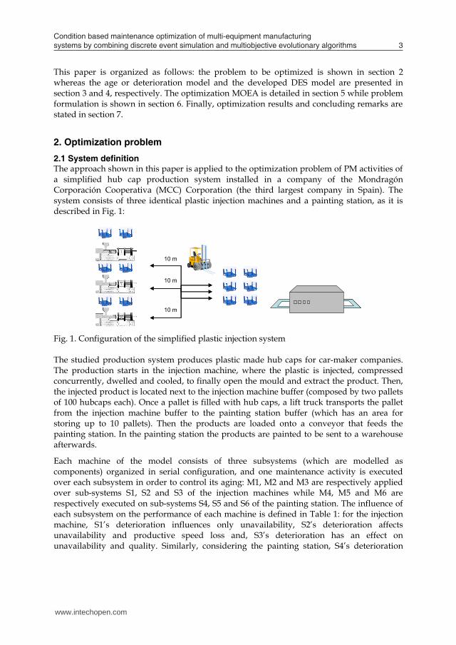
2.1 System definition The approach shown in this paper is applied to the optimization problem of PM activities of a simplified hub cap production system installed in a company of the Mondragón Corporación Cooperativa (MCC) Corporation (the third largest company in Spain). The system consists of three identical plastic injection machines and a painting station, as it is described in Fig. 1:
10 m
10 m
10 m
Fig. 1. Configuration of the simplified plastic injection system The studied production system produces plastic made hub caps for car-maker companies. The production starts in the injection machine, where the plastic is injected, compressed concurrently, dwelled and cooled, to finally open the mould and extract the product. Then, the injected product is located next to the injection machine buffer (composed by two pallets of 100 hubcaps each). Once a pallet is filled with hub caps, a lift truck transports the pallet from the injection machine buffer to the painting station buffer (which has an area for storing up to 10 pallets). Then the products are loaded onto a conveyor that feeds the painting station. In the painting station the products are painted to be sent to a warehouse afterwards.
Each machine of the model consists of three subsystems (which are modelled as components) organized in serial configuration, and one maintenance activity is executed over each subsystem in order to control its aging: M1, M2 and M3 are respectively applied over sub-systems S1, S2 and S3 of the injection machines while M4, M5 and M6 are respectively executed on sub-systems S4, S5 and S6 of the painting station. The influence of each subsystem on the performance of each machine is defined in Table 1: for the injection machine, S1’s deterioration influences only unavailability, S2’s deterioration affects unavailability and productive speed loss and, S3’s deterioration has an effect on unavailability and quality. Similarly, considering the painting station, S4’s deterioration
www.intechopen.com
Condition based maintenance optimization of multi-equipment manufacturing systems by combining discrete event simulation and multiobjective evolutionary algorithms 3
Keywords Maintenance, Optimization, Discrete Event Simulation, Multi-objective Evolutionary Algorithm.
1. Introduction
Industrial plant management, especially maintenance optimization, is usually characterized by the need to consider multiple non-commensurable and often conflicting objectives (see i.e. (Bader & Guesneux 2007;Goti & Sánchez 2006)). Equipment can be over maintained increasing preventive maintenance (PM) expenditures or under maintained increasing catastrophic failures. In these situations, and considering that maintenance requirements depend on many facts (whether the maintained equipment is a productive bottleneck, if it has a crucial impact in manufactured products’ quality, etc.), it is very difficult to determine the optimal maintenance strategy that maximizes the profitability of the studied equipment considering different criteria. In the latest years, many works have been presented devoted to find an optimal maintenance policy focused on different points of view, mainly oriented to the optimization of single deteriorating equipment and without taking into account the configuration of the productive system which contains the equipments to be maintained. Single equipment optimization approaches may be especially interesting when productive bottlenecks or continuous processes (such as foundries, rolling mills, etc.) are analyzed. Nevertheless, these initiatives might be less useful in manufacturing machines which work in multi-equipment systems, as they usually do not take into account the influence that the whole system has in each of the studied machines. Maintenance requirements related to a single machine of a multi-equipment system depend strongly the amount of semi-elaborated products’ stock related to the machine, whether it is a bottleneck or not, etc. For instance, if the studied machine is a bottleneck its availability will be crucial for the profitability of the company, whereas if not the impact of its failure will not be so important for the whole system (depending on stock levels and repair times (Li & Zuo 2007)). However, and although maintenance applied on equipment depends on the configuration of the system where the equipment is, little research can be found in the literature where a system composed by several equipments is optimized (Fiori de Castro & Lucchesi Cavalca 2006;Gharbi & Kenné 2005;Goyal & Kusy 1985;Grigoriev, van de Klunder, & Spieksma 2006;Kenne, Boukas, & Gharbi 2003;Yao 2005). This paper provides a solution for the joint optimization of CBM strategies applied on several equipments. Precisely, the research is focused on the problem of CMT optimization in a manufacturing environment with the objective of determining the optimal age or deterioration levels when a Preventive Maintenance (PM) action should be performed for multi-equipment systems under cost and profit criteria. The approach developed takes into account the interaction of production, work in process material, quality and maintenance aspects. For this purpose, a model that considers maintenance, productive speed loss and non-quality costs along with productive profit has been developed. The model has been implemented using Discrete Event Simulation (DES) and optimized using a Multiobjective Evolutionary Algorithm (MOEA). Thus, the suitability of DES to model or modify complex system models is combined with the aptitude that MOEAs have shown to deal with multiobjective problems.
This paper is organized as follows: the problem to be optimized is shown in section 2 whereas the age or deterioration model and the developed DES model are presented in section 3 and 4, respectively. The optimization MOEA is detailed in section 5 while problem formulation is shown in section 6. Finally, optimization results and concluding remarks are stated in section 7.
2. Optimization problem
2.1 System definition The approach shown in this paper is applied to the optimization problem of PM activities of a simplified hub cap production system installed in a company of the Mondragón Corporación Cooperativa (MCC) Corporation (the third largest company in Spain). The system consists of three identical plastic injection machines and a painting station, as it is described in Fig. 1:
10 m
10 m
10 m
Fig. 1. Configuration of the simplified plastic injection system The studied production system produces plastic made hub caps for car-maker companies. The production starts in the injection machine, where the plastic is injected, compressed concurrently, dwelled and cooled, to finally open the mould and extract the product. Then, the injected product is located next to the injection machine buffer (composed by two pallets of 100 hubcaps each). Once a pallet is filled with hub caps, a lift truck transports the pallet from the injection machine buffer to the painting station buffer (which has an area for storing up to 10 pallets). Then the products are loaded onto a conveyor that feeds the painting station. In the painting station the products are painted to be sent to a warehouse afterwards.
Each machine of the model consists of three subsystems (which are modelled as components) organized in serial configuration, and one maintenance activity is executed over each subsystem in order to control its aging: M1, M2 and M3 are respectively applied over sub-systems S1, S2 and S3 of the injection machines while M4, M5 and M6 are respectively executed on sub-systems S4, S5 and S6 of the painting station. The influence of each subsystem on the performance of each machine is defined in Table 1: for the injection machine, S1’s deterioration influences only unavailability, S2’s deterioration affects unavailability and productive speed loss and, S3’s deterioration has an effect on unavailability and quality. Similarly, considering the painting station, S4’s deterioration
www.intechopen.com

influences only unavailability, S5’s deterioration affects unavailability and productive speed loss and, S6’s deterioration has an effect on unavailability and quality.
Maintained equipment
Name of the PM activity executed
when the age of its corresponding
subsystem achieves an age
Subsystem Influences on
Injection machines
M1 S1 Unavailability M2 S2 Unavailability and
Productive speed loss M3 S3 Unavailability and Quality
Painting station
M4 S4 Unavailability M5 S5 Unavailability and
Productive speed loss M6 S6 Unavailability and Quality
Table 1. System components, PM activities and their influences on productive parameters The equipments failure process is modeled by using a two-parameter (1, 1) Weibull failure rate. Additionally, it is considered that the production process can be subject to a process deterioration that shifts the system from an under-control state to an out-of-control state. This process deterioration follows also a Weibull distribution of parameters 2, 2. Table 2 shows the Weibull reliability data for the studied problem.
Group 1(10-2hrs-1) 1 2(10-2hrs-1) 2 S1 5 2 S2 2 2.9 S3 4 2 4 2 S4 6.6 2 S5 7.7 3 S6 10 3 10 3
Table 2. Weibull data of the studied subsystems
3. Deterioration or reliability model
3.1 Deterioration model Traditionally, the effect of the maintenance activities on the state of a equipment is based on three situations: a) perfect maintenance activity which assumes that the state of the component after the maintenance is “As Good as New” (GAN), b) minimal maintenance which supposes that activity leaves the equipment in “As Bad as Old” (BAO) situation, and c) imperfect maintenance which assumes that the activity improves the state of the equipment by some degree depending on its effectiveness. Last situation is closer to many real situations.
There exist several models developed to simulate imperfect maintenance (Chan & Shaw 1993;Malik 1979;Shin, Lim, & Lie 1996). In this paper, an age reduction preventive maintenance model, named Proportional Age-Set Back (PAS), proposed by Martorell et al. ( 1999) is used to model the effect of the maintenance activities on the equipment. In the PAS approach, each maintenance activity is assumed to shift the origin of time from which the age of the component is evaluated. PAS model in Ref. (Martorell, Sánchez, & Serradell 1998) considers that the maintenance activity reduces proportionally, in a factor of , the age that the component has immediately before it enters maintenance, where ranges in the interval [0,1]. If 0 , the PAS model simply reduces to a BAO situation, while if
1 it is reduced to a GAN situation. Thus, this model is a natural generalization of both GAN and BAO models in order to account for imperfect maintenance. Based on Ref (Martorell et al. 1999), the age of the component immediately after the (m-1)-maintenance
activity ( 1-mw ) is given by:
)tεε)(1(tw2m
0k1-km
k1-m1-m (1)
where 1mt is the time in which the component undertakes the m-1 maintenance activity
As Sherif & Smith ( 1981) state, if it is assumed that a probability distribution of the time to failure is available, risk can be measured. Risks associated to degradation in monitoring equipment consider poor quality and performance, productive breakdowns related to Corrective Maintenance (CM), etc. The following paragraphs go deep into the modelling of such risks. Considering a CMT strategy, PM is performed when the component gets a determined
critical age or deterioration level ( cw ). It is worth to remember that PAS model considers that the maintenance reduces proportionally, in a factor, the age that the component has immediately before it enters maintenance. Considering these conditions, maintenance always will be applied to a component when it has the same age, and as effectiveness is assumed to be constant the age of the component will always be the same after performing a
PM action. This means that mw and
mw , which represent respectively the age of the component just before and after the mth PM intervention, will always get the same values:
cm ww (2)
cm wε1w (3) As a consequence, the time interval M between two PM activities will have this value:
εwM c (4)
www.intechopen.com

Condition based maintenance optimization of multi-equipment manufacturing systems by combining discrete event simulation and multiobjective evolutionary algorithms 5
influences only unavailability, S5’s deterioration affects unavailability and productive speed loss and, S6’s deterioration has an effect on unavailability and quality.
Maintained equipment
Name of the PM activity executed
when the age of its corresponding
subsystem achieves an age
Subsystem Influences on
Injection machines
M1 S1 Unavailability M2 S2 Unavailability and
Productive speed loss M3 S3 Unavailability and Quality
Painting station
M4 S4 Unavailability M5 S5 Unavailability and
Productive speed loss M6 S6 Unavailability and Quality
Table 1. System components, PM activities and their influences on productive parameters The equipments failure process is modeled by using a two-parameter (1, 1) Weibull failure rate. Additionally, it is considered that the production process can be subject to a process deterioration that shifts the system from an under-control state to an out-of-control state. This process deterioration follows also a Weibull distribution of parameters 2, 2. Table 2 shows the Weibull reliability data for the studied problem.
Group 1(10-2hrs-1) 1 2(10-2hrs-1) 2 S1 5 2 S2 2 2.9 S3 4 2 4 2 S4 6.6 2 S5 7.7 3 S6 10 3 10 3
Table 2. Weibull data of the studied subsystems
3. Deterioration or reliability model
3.1 Deterioration model Traditionally, the effect of the maintenance activities on the state of a equipment is based on three situations: a) perfect maintenance activity which assumes that the state of the component after the maintenance is “As Good as New” (GAN), b) minimal maintenance which supposes that activity leaves the equipment in “As Bad as Old” (BAO) situation, and c) imperfect maintenance which assumes that the activity improves the state of the equipment by some degree depending on its effectiveness. Last situation is closer to many real situations.
There exist several models developed to simulate imperfect maintenance (Chan & Shaw 1993;Malik 1979;Shin, Lim, & Lie 1996). In this paper, an age reduction preventive maintenance model, named Proportional Age-Set Back (PAS), proposed by Martorell et al. ( 1999) is used to model the effect of the maintenance activities on the equipment. In the PAS approach, each maintenance activity is assumed to shift the origin of time from which the age of the component is evaluated. PAS model in Ref. (Martorell, Sánchez, & Serradell 1998) considers that the maintenance activity reduces proportionally, in a factor of , the age that the component has immediately before it enters maintenance, where ranges in the interval [0,1]. If 0 , the PAS model simply reduces to a BAO situation, while if
1 it is reduced to a GAN situation. Thus, this model is a natural generalization of both GAN and BAO models in order to account for imperfect maintenance. Based on Ref (Martorell et al. 1999), the age of the component immediately after the (m-1)-maintenance
activity ( 1-mw ) is given by:
)tεε)(1(tw2m
0k1-km
k1-m1-m (1)
where 1mt is the time in which the component undertakes the m-1 maintenance activity
As Sherif & Smith ( 1981) state, if it is assumed that a probability distribution of the time to failure is available, risk can be measured. Risks associated to degradation in monitoring equipment consider poor quality and performance, productive breakdowns related to Corrective Maintenance (CM), etc. The following paragraphs go deep into the modelling of such risks. Considering a CMT strategy, PM is performed when the component gets a determined
critical age or deterioration level ( cw ). It is worth to remember that PAS model considers that the maintenance reduces proportionally, in a factor, the age that the component has immediately before it enters maintenance. Considering these conditions, maintenance always will be applied to a component when it has the same age, and as effectiveness is assumed to be constant the age of the component will always be the same after performing a
PM action. This means that mw and
mw , which represent respectively the age of the component just before and after the mth PM intervention, will always get the same values:
cm ww (2)
cm wε1w (3) As a consequence, the time interval M between two PM activities will have this value:
εwM c (4)
www.intechopen.com

3.2 Reliability model Using Equations 2-4, it is possible to obtain an age-dependent reliability model in which the induced or conditional failure rate, in the period m, after the maintenance number m, given by: h))(t,(wh))(t,(wh 0mmm (5) where h0 represents the initial failure rate of the component, that is, the one that equipment has when it installed. Considering the age of the component after maintenance m given by Equation 1, and adopting a Weibull model for the failure rate, the expression for the induced failure rate after the maintenance number m can be written as:
01γ
mγ
mm h)(t,wγλ))(t,(wh (6)
where is the scale parameter, is known as the shape parameter. The behaviour of
))(t,(wh mm function fluctuates between two values as was observed for the age of the component and its maximum and minimum values are given by:
γ 1γ- -m m 0h λ γ w h
(7)
γ 1γm m 0h λ γ w h
(8)
Then, in order to introduce the effect of maintenance activities into the cost and profit models, to be presented in the following section, it is derived an averaged standby failure rate over the component’s life based on a double averaging process. First, it is formulated
*mh the average failure rate over the period between two consecutive maintenance
activities, m and m+1. Next, it is formulated the average failure rate, *h , over the analysis
period, L, which is practically equal to *mh . Thus is:
01
t
tm+
m-
1m
*m
h11M
(t).dthtt
1hh-
1m
+m
(9)
3.3 Availability model As a consequence of what it is explained in the previous subsection, and based on Ref. (Martorell, Serradell, & Samanta 1995), xru , the time-dependent unreliability for discontinuous equipment can be calculated as:
M.hr
*
e1.1u x (10)
where is the probability of failure on demand, and h* is evaluated using Equation 10. Then xU is the total unavailability of the studied system evaluated using the system fault tree
and the single component unavailability contributions. These contributions are xcmu which is the unavailability due to CM given by:
cmrcm dMxuM1u ,x (11)
Where dcm is the mean time for CM; and xpmu that represents the unavailability
associated to the PM interventions launched due to CMT monitoring in the L period. Considering the periodicity of the PM activities explained in Equation 4, xpmu is given
by:
pmpm dM1u x (12)
Where dpm the mean time for PM; Finally, the total availability of the studied system xA is evaluated as: xx U1A (13) being U(x) the system unavailability to be evaluated using the system fault tree and the single component corrective and preventive maintenance unavailability contributions.
4. Discrete event simulation model
DES concerns the modeling of a system as it evolves over time by a representation in which variable states change suddenly at separate points in time, as it is detailed in the other chapter of this book authored by the same author. These changes happened in the system are considered events. Systems do not change between events, so DES considers that it is not necessary to analyze what happens in a system in periods taken place between two events. The main advantages of DES are two: i) standard DES-based tools provide capabilities of modeling or modifying complex system models easily, and ii) DES is closely related to stochastic systems so they are appropriate when simulating real-world phenomena, since there are few situations where the actions of the entities within the system under study can be completely predicted in advance. In order to generate stochastic events, simulation packages generate pseudo-random numbers to select a particular value for a given distribution. Similarly, equations related to analytical models (i.e. breakdown models) can also be implemented due to the generation of these pseudo-random numbers. Thus, using pseudo-random numbers it is possible to implement the stochastic nature of real models in DES models.
www.intechopen.com

Condition based maintenance optimization of multi-equipment manufacturing systems by combining discrete event simulation and multiobjective evolutionary algorithms 7
3.2 Reliability model Using Equations 2-4, it is possible to obtain an age-dependent reliability model in which the induced or conditional failure rate, in the period m, after the maintenance number m, given by: h))(t,(wh))(t,(wh 0mmm (5) where h0 represents the initial failure rate of the component, that is, the one that equipment has when it installed. Considering the age of the component after maintenance m given by Equation 1, and adopting a Weibull model for the failure rate, the expression for the induced failure rate after the maintenance number m can be written as:
01γ
mγ
mm h)(t,wγλ))(t,(wh (6)
where is the scale parameter, is known as the shape parameter. The behaviour of
))(t,(wh mm function fluctuates between two values as was observed for the age of the component and its maximum and minimum values are given by:
γ 1γ- -m m 0h λ γ w h
(7)
γ 1γm m 0h λ γ w h
(8)
Then, in order to introduce the effect of maintenance activities into the cost and profit models, to be presented in the following section, it is derived an averaged standby failure rate over the component’s life based on a double averaging process. First, it is formulated
*mh the average failure rate over the period between two consecutive maintenance
activities, m and m+1. Next, it is formulated the average failure rate, *h , over the analysis
period, L, which is practically equal to *mh . Thus is:
01
t
tm+
m-
1m
*m
h11M
(t).dthtt
1hh-
1m
+m
(9)
3.3 Availability model As a consequence of what it is explained in the previous subsection, and based on Ref. (Martorell, Serradell, & Samanta 1995), xru , the time-dependent unreliability for discontinuous equipment can be calculated as:
M.hr
*
e1.1u x (10)
where is the probability of failure on demand, and h* is evaluated using Equation 10. Then xU is the total unavailability of the studied system evaluated using the system fault tree
and the single component unavailability contributions. These contributions are xcmu which is the unavailability due to CM given by:
cmrcm dMxuM1u ,x (11)
Where dcm is the mean time for CM; and xpmu that represents the unavailability
associated to the PM interventions launched due to CMT monitoring in the L period. Considering the periodicity of the PM activities explained in Equation 4, xpmu is given
by:
pmpm dM1u x (12)
Where dpm the mean time for PM; Finally, the total availability of the studied system xA is evaluated as: xx U1A (13) being U(x) the system unavailability to be evaluated using the system fault tree and the single component corrective and preventive maintenance unavailability contributions.
4. Discrete event simulation model
DES concerns the modeling of a system as it evolves over time by a representation in which variable states change suddenly at separate points in time, as it is detailed in the other chapter of this book authored by the same author. These changes happened in the system are considered events. Systems do not change between events, so DES considers that it is not necessary to analyze what happens in a system in periods taken place between two events. The main advantages of DES are two: i) standard DES-based tools provide capabilities of modeling or modifying complex system models easily, and ii) DES is closely related to stochastic systems so they are appropriate when simulating real-world phenomena, since there are few situations where the actions of the entities within the system under study can be completely predicted in advance. In order to generate stochastic events, simulation packages generate pseudo-random numbers to select a particular value for a given distribution. Similarly, equations related to analytical models (i.e. breakdown models) can also be implemented due to the generation of these pseudo-random numbers. Thus, using pseudo-random numbers it is possible to implement the stochastic nature of real models in DES models.
www.intechopen.com

The DES model simulates the injection machines, the painting station, the lift, the product buffers and its pallets. The implementation of each of these components is detailed in the following subsections.
4.1 Equipment modeling The behavior pattern of the machines represented in the DES model bases on an analytical model. This model is presented in ( 2006). In that work a single equipment model is detailed. The paper models maintenance, quality and production speed loss costs jointly with the benefit related to the production of non-defective products. All of these terms depend on the PM activities performed, which act as decision variables (x) and are optimized under cost and profit criteria. That equipment model was developed considering the following assumptions: 1) the effect of the maintenance activities is modeled by using an imperfect maintenance model. In this case a Proportional Age Set-Back (Martorell, Sánchez, & Serradell 1999) is assumed, 2) the failure process and deterioration process are independent, 3) the system only produces non-conforming items, with a rate constant (), while the process is out-of-control, 4) Preventive maintenance and process inspection are performed simultaneously, 5) inspections are error free and 6) the process is restored to under control state when the preventive maintenance is realized, 7) productive speed is assumed to fall from its initial speed (V0) to another speed value (V*(x)) which depends on the PM frequency, 8) as in (Li & Pham 2005), we assume that all the deterioration processes of the three studied components are independent, and 9) it is assumed that the process produces a single product type, so setup times of reference changes are not simulated. The relevant productive parameters of the described equipment model include: i) direct maintenance parameters, ii) quality parameters and iii) productive speed loss parameters. These parameters can be evaluated as:
ε2
2-εMτVV 0x* (14)
Mxh*M
0m
* *
eh21dwεt,wft
M1xκ (15)
Where; V*(x) the mean production speed of the equipment during the L period; and *(x) the mean fraction of time where the process is under control. In addition, the following notation is used: V0 the initial (e.g. as per design) production speed; the speed loss coefficient; the cyclic or per-demand failure probability; and fm(w(t,)) the density function obtained using the conditional hazard function. In this research, analytical formulation corresponding to each machine of the productive system is implemented within the equipment to generate stochastic events that make equipment work as it is defined in the analytical model. This integration is performed in two steps: first the components of the decision vector related to the studied machines are evaluated analytically, obtaining the working parameters Ucm(x), Upm(x), V*(x) and *(x) of the corresponding PM frequencies (where Ucm(x) and Upm(x) are respectively the
unavailability of a machine due to CM and PM, evaluated using the system fault tree and the single component ucm(x) and upm(x) contributions). In a second step, the generated working parameters are introduced as inputs in the DES modelled machines to execute then a simulation where the results to be optimised are obtained. The implementation of values obtained in the analytical evaluation executed in the DES model derives in the generation of planned PM, unplanned CM, speed reduction and defective product actions and events during the simulation. As a consequence, at the end of the simulation machines generate the same values of Ucm(x), Upm(x) and *(x) defined by the analytical model to produce items in a V*(x) productive speed. Fig. 2 shows the generation of unavailability, speed loss and quality events for an equipment during a simulation:
Maintained
States
Operative
t
Events
PM performed
Failure
M
PM performed
CM performed
Under control
Out of control
M.*
Defective product
M.(1-*)
Production of an item
starts
Production of an item finishes
1/V0
1/V*
Maintained
States
Operative
t
Events
PM performed
Failure
M
PM performed
CM performed
Under control
Out of control
M.*
Defective product
M.(1-*)
Production of an item
starts
Production of an item finishes
1/V0
1/V*
Fig. 2. Generation of events related to maintenance, productive speed and quality As it can be seen in Fig. 2 events related to PM are generated with a determined periodicity (M) and each product needs a 1/V* cycle time to be produced. Failures are generated randomly to obtain an unavailability related to CM which is equal to Ucm(x). Referred to quality, there are no defective products during the first *(x) fraction between two PM activities, while there is a defective fraction during the following (1-*(x)) fraction. Thus, thanks to the interaction between analytical evaluation and DES modelling simulation equipments work as it is defined in analytical models shown in Eqns. (14 – 15). Additionally,
www.intechopen.com

Condition based maintenance optimization of multi-equipment manufacturing systems by combining discrete event simulation and multiobjective evolutionary algorithms 9
The DES model simulates the injection machines, the painting station, the lift, the product buffers and its pallets. The implementation of each of these components is detailed in the following subsections.
4.1 Equipment modeling The behavior pattern of the machines represented in the DES model bases on an analytical model. This model is presented in ( 2006). In that work a single equipment model is detailed. The paper models maintenance, quality and production speed loss costs jointly with the benefit related to the production of non-defective products. All of these terms depend on the PM activities performed, which act as decision variables (x) and are optimized under cost and profit criteria. That equipment model was developed considering the following assumptions: 1) the effect of the maintenance activities is modeled by using an imperfect maintenance model. In this case a Proportional Age Set-Back (Martorell, Sánchez, & Serradell 1999) is assumed, 2) the failure process and deterioration process are independent, 3) the system only produces non-conforming items, with a rate constant (), while the process is out-of-control, 4) Preventive maintenance and process inspection are performed simultaneously, 5) inspections are error free and 6) the process is restored to under control state when the preventive maintenance is realized, 7) productive speed is assumed to fall from its initial speed (V0) to another speed value (V*(x)) which depends on the PM frequency, 8) as in (Li & Pham 2005), we assume that all the deterioration processes of the three studied components are independent, and 9) it is assumed that the process produces a single product type, so setup times of reference changes are not simulated. The relevant productive parameters of the described equipment model include: i) direct maintenance parameters, ii) quality parameters and iii) productive speed loss parameters. These parameters can be evaluated as:
ε2
2-εMτVV 0x* (14)
Mxh*M
0m
* *
eh21dwεt,wft
M1xκ (15)
Where; V*(x) the mean production speed of the equipment during the L period; and *(x) the mean fraction of time where the process is under control. In addition, the following notation is used: V0 the initial (e.g. as per design) production speed; the speed loss coefficient; the cyclic or per-demand failure probability; and fm(w(t,)) the density function obtained using the conditional hazard function. In this research, analytical formulation corresponding to each machine of the productive system is implemented within the equipment to generate stochastic events that make equipment work as it is defined in the analytical model. This integration is performed in two steps: first the components of the decision vector related to the studied machines are evaluated analytically, obtaining the working parameters Ucm(x), Upm(x), V*(x) and *(x) of the corresponding PM frequencies (where Ucm(x) and Upm(x) are respectively the
unavailability of a machine due to CM and PM, evaluated using the system fault tree and the single component ucm(x) and upm(x) contributions). In a second step, the generated working parameters are introduced as inputs in the DES modelled machines to execute then a simulation where the results to be optimised are obtained. The implementation of values obtained in the analytical evaluation executed in the DES model derives in the generation of planned PM, unplanned CM, speed reduction and defective product actions and events during the simulation. As a consequence, at the end of the simulation machines generate the same values of Ucm(x), Upm(x) and *(x) defined by the analytical model to produce items in a V*(x) productive speed. Fig. 2 shows the generation of unavailability, speed loss and quality events for an equipment during a simulation:
Maintained
States
Operative
t
Events
PM performed
Failure
M
PM performed
CM performed
Under control
Out of control
M.*
Defective product
M.(1-*)
Production of an item
starts
Production of an item finishes
1/V0
1/V*
Maintained
States
Operative
t
Events
PM performed
Failure
M
PM performed
CM performed
Under control
Out of control
M.*
Defective product
M.(1-*)
Production of an item
starts
Production of an item finishes
1/V0
1/V*
Fig. 2. Generation of events related to maintenance, productive speed and quality As it can be seen in Fig. 2 events related to PM are generated with a determined periodicity (M) and each product needs a 1/V* cycle time to be produced. Failures are generated randomly to obtain an unavailability related to CM which is equal to Ucm(x). Referred to quality, there are no defective products during the first *(x) fraction between two PM activities, while there is a defective fraction during the following (1-*(x)) fraction. Thus, thanks to the interaction between analytical evaluation and DES modelling simulation equipments work as it is defined in analytical models shown in Eqns. (14 – 15). Additionally,
www.intechopen.com

and thanks to the capability of combining different machines in a system, the DES model not only models the features of a single machine, but the interaction among several machines. The generation of each one of the above mentioned events is related to a specific inefficiency so their costs have to be taken into account. Costs are quantified considering CM, PM, speed loss, quality and CMT terms. In order to do that, individual cost counters related each one of these terms (ccm(x), cpm(x), csl(x), cq(x) and ccmt(x), respectively) are defined; these counters are initialized to zero at the beginning of the simulation and increased every time an event related to them is generated by the simulation using Eqns. (16 – 20): hcmcmcmcm cdcc (x)(x) (16)
hpmpmpmpm cdcc (x)(x) (17)
hsl0slsl cV1V1cc /(x)/(x)(x) * (18)
ccc qq (x)(x) (19)
Lc(x)c hcmtcmt (20) where chcm, chpm, chsl and chcmt represent respectively the hourly cost related to the CM, the PM, the reduced speed and the CMT, while c represents the cost of manufacturing a defective product. Finally, P(x) characterizes the profit function obtained as a result of selling non-defective products, which can be evaluated as: ψnP (x)x (21) where n(x) represents the amount of non-defective products obtained during the analysis period (L), and is the estimated margin of a single product.
4.2 Buffer and transportation modeling System buffers have a determined maximum capacity. The model assumes that if a buffer is full it will not receive any products until it has free pallets to store them (so the transportation events will not be executed). This means also that a machine will stop producing products in case it does not have any place to leave them. The painting station is fed by a buffer of ten pallets, being each one capable of storing 100 products, whereas each injection machine feeds a buffer of two pallets of 100 each. Referred to transportation modeling, only semi-elaborated product movements have been modeled, considering movements between: i) a machine and a buffer location, ii) two machines, iii) a buffer location and a machine, and iv) two buffer locations. It is worth to note that for transportation types i), ii) and iii) products are moved one by one, whereas for movements between two buffer locations products are transported in pallets. All of these movements are modeled by introducing a delay in the system. Thus, in instant t the element is at the initial point, to be at the destination point in instant t+delay. For sake of simplicity transportation types i), ii) and iii) are not modeled (delay=0), whereas injection machines are fed with empty pallets and empty pallets of the painting station are removed from the
system automatically and instantaneously. The lift truck transport is modeled using a delay which has a uniform distribution range between 14.4 and 28.8 s.
4.3 Simulation values of the productive system Data collected for the simulation model is shown in the next 4 tables. Tables 3 and 4 show parameters related to PM and CM, whereas Tables 5 and 6 detail respectively information about inputs related to CM, unavailability, speed, quality and cost for the injection machines and the painting station.
Preventive maintenance
activity
dpm (hrs)
M1 0.9 0.5 M2 0.9 1 M3 0.9 1 M4 0.9 2 M5 0.9 1 M6 0.9 3
Table 3. PM data related to the productive system
Corrective breakdown of sub-system
dcm (hrs)
S1 0.5 S2 1 S3 2 S4 0.5 S5 1 S6 2
Table 4. CM data related to the productive system
C
(€/u1)
(u/h2) Chsl
(€/hr)
(10-
3)
h0 (fail/hr)
V0
(u/hr) chcm
(€/hr) chpm
(€/hr) chcmt
(€/hr)
6 0.0017 25 1 0.03 0 180 45 30 1 Table 5. Productive and cost parameters for the injection machines
C
(€/u)
(u/h2) Chsl
(€/hr)
(10-
3)
h0 (fail/hr)
V0
(u/hr) chcm
(€/hr) chpm
(€/hr) chcmt
(€/hr)
6 0.02 150 1 0.04 0 900 175 160 1 Table 6. Productive and cost parameters for the painting station
1 Where u represents a product unit
www.intechopen.com

Condition based maintenance optimization of multi-equipment manufacturing systems by combining discrete event simulation and multiobjective evolutionary algorithms 11
and thanks to the capability of combining different machines in a system, the DES model not only models the features of a single machine, but the interaction among several machines. The generation of each one of the above mentioned events is related to a specific inefficiency so their costs have to be taken into account. Costs are quantified considering CM, PM, speed loss, quality and CMT terms. In order to do that, individual cost counters related each one of these terms (ccm(x), cpm(x), csl(x), cq(x) and ccmt(x), respectively) are defined; these counters are initialized to zero at the beginning of the simulation and increased every time an event related to them is generated by the simulation using Eqns. (16 – 20): hcmcmcmcm cdcc (x)(x) (16)
hpmpmpmpm cdcc (x)(x) (17)
hsl0slsl cV1V1cc /(x)/(x)(x) * (18)
ccc qq (x)(x) (19)
Lc(x)c hcmtcmt (20) where chcm, chpm, chsl and chcmt represent respectively the hourly cost related to the CM, the PM, the reduced speed and the CMT, while c represents the cost of manufacturing a defective product. Finally, P(x) characterizes the profit function obtained as a result of selling non-defective products, which can be evaluated as: ψnP (x)x (21) where n(x) represents the amount of non-defective products obtained during the analysis period (L), and is the estimated margin of a single product.
4.2 Buffer and transportation modeling System buffers have a determined maximum capacity. The model assumes that if a buffer is full it will not receive any products until it has free pallets to store them (so the transportation events will not be executed). This means also that a machine will stop producing products in case it does not have any place to leave them. The painting station is fed by a buffer of ten pallets, being each one capable of storing 100 products, whereas each injection machine feeds a buffer of two pallets of 100 each. Referred to transportation modeling, only semi-elaborated product movements have been modeled, considering movements between: i) a machine and a buffer location, ii) two machines, iii) a buffer location and a machine, and iv) two buffer locations. It is worth to note that for transportation types i), ii) and iii) products are moved one by one, whereas for movements between two buffer locations products are transported in pallets. All of these movements are modeled by introducing a delay in the system. Thus, in instant t the element is at the initial point, to be at the destination point in instant t+delay. For sake of simplicity transportation types i), ii) and iii) are not modeled (delay=0), whereas injection machines are fed with empty pallets and empty pallets of the painting station are removed from the
system automatically and instantaneously. The lift truck transport is modeled using a delay which has a uniform distribution range between 14.4 and 28.8 s.
4.3 Simulation values of the productive system Data collected for the simulation model is shown in the next 4 tables. Tables 3 and 4 show parameters related to PM and CM, whereas Tables 5 and 6 detail respectively information about inputs related to CM, unavailability, speed, quality and cost for the injection machines and the painting station.
Preventive maintenance
activity
dpm (hrs)
M1 0.9 0.5 M2 0.9 1 M3 0.9 1 M4 0.9 2 M5 0.9 1 M6 0.9 3
Table 3. PM data related to the productive system
Corrective breakdown of sub-system
dcm (hrs)
S1 0.5 S2 1 S3 2 S4 0.5 S5 1 S6 2
Table 4. CM data related to the productive system
C
(€/u1)
(u/h2) Chsl
(€/hr)
(10-
3)
h0 (fail/hr)
V0
(u/hr) chcm
(€/hr) chpm
(€/hr) chcmt
(€/hr)
6 0.0017 25 1 0.03 0 180 45 30 1 Table 5. Productive and cost parameters for the injection machines
C
(€/u)
(u/h2) Chsl
(€/hr)
(10-
3)
h0 (fail/hr)
V0
(u/hr) chcm
(€/hr) chpm
(€/hr) chcmt
(€/hr)
6 0.02 150 1 0.04 0 900 175 160 1 Table 6. Productive and cost parameters for the painting station
1 Where u represents a product unit
www.intechopen.com

Additionally, the net profit value of a non-defective product () is 0.2 €/unit and the simulation time L is 62400 working hours, which corresponds to 10 years of production working 5 days a week and 24 hours a day.
Finally, the time required to execute a simulation in DES increases in an exponential way compared to the complexity of the studied model (Oyarbide-Zubillaga, Baines, & Kay 2003). For this reason and in order to reduce the time which the simulation is being executed products are elaborated in batches of 100 units.
5. The NSGA-II multiobjective evolutionary algorithm
In this approach the Non-dominated Sorting Genetic Algorithm (NSGA-II) proposed by Deb et al. (2002) has been implemented. The NSGA-II is the most recent and improved version of the NSGA which incorporates: a) a faster non-dominated sorting approach, b) an elitist strategy i.e. the best non-dominated individuals are preserved from one generation to another by using a crowding measurement, and c) no niching parameter. This algorithm is capable of performing a joint optimization under several criteria offering non-dominated solutions. The non-dominated results are situated in a Pareto optimal front, where each of the solutions is better than any other solution of the front at least in one of the studied optimization criterion. The working procedure of the NSGA-II is shown in Fig. 3 and detailed in the following steps:
Combine previous
Qi and result Pigenerations*
Qt= Pi Qi
StartStart
Create initial
population Pi
Fitness value calculation of the
new genes
Convergence?
No
Yes
EndEnd
Results
Fronts calculation
F1,F2,…,Fkaccording to non-
dominance
Crowding distance calculation of each
solution of Fi for each front
Choose the N best individuals to
create Pi+1
Binary selection, scattered crossover and random gene mutation to create
offspring
population Qi+1
i = i +1
* Qt= Pi
if i =1
i=1
Fig. 3. Working procedure of the NSGA-II
Step 1. Fix N, i=1, and imax. N = population size i = number of generations imax = maximum number of interactions of the genetic algorithm
Step 2. Create and evaluate a random parent population Pi of size N. Step 3. If i=imaxGA return Pi else: Step 4. Form a combined population of size 2N as Ti= Pi Qi.
Qi = offspring population Ti size N and equal to Pi in the first interaction
Step 5. Ranking (according to restriction violations). Step 6. Identify non dominated fronts F1, F2, …., Fk. Thus an each solution is assigned a
fitness equal to its non-domination level. Step 7. Create Pi+1 as the N best individuals from Pi. Step 8. Select randomly N couples from Pi+1 using a binary tournament selection. Step 9. Create offspring population Qi+1 applying crossover and mutation (size N). Step 10. Evaluate the offspring population. Step 11. Do i=i+1. Step 12. Go to step 4.
Following the procedure detailed above the algorithm evaluates the x1, x2, …, xN genes of each generation. In this case, to obtain the respective f(x1), f(x2), …, f(xN) fitness values of the evaluation, the DES model performs a simulation where PM frequencies act as decision variables to obtain economic parameters.
6. Problem formulation
The optimization of preventive maintenance activities based on cost and benefit criteria can be formulated as a multi-objective optimization problem (MOP). A general MOP includes a set of parameters (decision variables), a set of objective functions, and a set of constraints. Objective functions and constraints are defined in terms of the decision variables using the models presented in the previous section. The optimization goal can be formulated to optimize a vector of functions of the form (Martorell et al. 2004): x,...,x,xxy n21 ffff (22) subject to the vector of constraints ))(g),...,(g),(g()(g n21 xxxx (23)
where Xx,...,x,xx n21 (24)
Yy,...,y,yy n21 (25)
www.intechopen.com

Condition based maintenance optimization of multi-equipment manufacturing systems by combining discrete event simulation and multiobjective evolutionary algorithms 13
Additionally, the net profit value of a non-defective product () is 0.2 €/unit and the simulation time L is 62400 working hours, which corresponds to 10 years of production working 5 days a week and 24 hours a day.
Finally, the time required to execute a simulation in DES increases in an exponential way compared to the complexity of the studied model (Oyarbide-Zubillaga, Baines, & Kay 2003). For this reason and in order to reduce the time which the simulation is being executed products are elaborated in batches of 100 units.
5. The NSGA-II multiobjective evolutionary algorithm
In this approach the Non-dominated Sorting Genetic Algorithm (NSGA-II) proposed by Deb et al. (2002) has been implemented. The NSGA-II is the most recent and improved version of the NSGA which incorporates: a) a faster non-dominated sorting approach, b) an elitist strategy i.e. the best non-dominated individuals are preserved from one generation to another by using a crowding measurement, and c) no niching parameter. This algorithm is capable of performing a joint optimization under several criteria offering non-dominated solutions. The non-dominated results are situated in a Pareto optimal front, where each of the solutions is better than any other solution of the front at least in one of the studied optimization criterion. The working procedure of the NSGA-II is shown in Fig. 3 and detailed in the following steps:
Combine previous
Qi and result Pigenerations*
Qt= Pi Qi
StartStart
Create initial
population Pi
Fitness value calculation of the
new genes
Convergence?
No
Yes
EndEnd
Results
Fronts calculation
F1,F2,…,Fkaccording to non-
dominance
Crowding distance calculation of each
solution of Fi for each front
Choose the N best individuals to
create Pi+1
Binary selection, scattered crossover and random gene mutation to create
offspring
population Qi+1
i = i +1
* Qt= Pi
if i =1
i=1
Fig. 3. Working procedure of the NSGA-II
Step 1. Fix N, i=1, and imax. N = population size i = number of generations imax = maximum number of interactions of the genetic algorithm
Step 2. Create and evaluate a random parent population Pi of size N. Step 3. If i=imaxGA return Pi else: Step 4. Form a combined population of size 2N as Ti= Pi Qi.
Qi = offspring population Ti size N and equal to Pi in the first interaction
Step 5. Ranking (according to restriction violations). Step 6. Identify non dominated fronts F1, F2, …., Fk. Thus an each solution is assigned a
fitness equal to its non-domination level. Step 7. Create Pi+1 as the N best individuals from Pi. Step 8. Select randomly N couples from Pi+1 using a binary tournament selection. Step 9. Create offspring population Qi+1 applying crossover and mutation (size N). Step 10. Evaluate the offspring population. Step 11. Do i=i+1. Step 12. Go to step 4.
Following the procedure detailed above the algorithm evaluates the x1, x2, …, xN genes of each generation. In this case, to obtain the respective f(x1), f(x2), …, f(xN) fitness values of the evaluation, the DES model performs a simulation where PM frequencies act as decision variables to obtain economic parameters.
6. Problem formulation
The optimization of preventive maintenance activities based on cost and benefit criteria can be formulated as a multi-objective optimization problem (MOP). A general MOP includes a set of parameters (decision variables), a set of objective functions, and a set of constraints. Objective functions and constraints are defined in terms of the decision variables using the models presented in the previous section. The optimization goal can be formulated to optimize a vector of functions of the form (Martorell et al. 2004): x,...,x,xxy n21 ffff (22) subject to the vector of constraints ))(g),...,(g),(g()(g n21 xxxx (23)
where Xx,...,x,xx n21 (24)
Yy,...,y,yy n21 (25)
www.intechopen.com
and x is the decision vector (vector of decision variables), y the objective vector, X the decision space and Y is the objective space, that is to say Y=f(X). The optimization of PM activities proposed in this paper considers the productive costs and profit as optimization criteria. Both cost and profit models depend on maintenance intervals, which act as decision variables and are encoded in the decision vector, x. So, the vector of bi-objective function, f(x), is defined as: x,x)x( PCf (26) where the objective is to minimize the function C(x) and maximize a profit function P(x). C(x) is the cost system which is evaluated as sum of the maintenance, production speed lost and quality costs for each of the m machines of the system which are evaluated using Eqns. (16 - 20).
C(x) m
1iiqislipmicm cccc xxxx (27)
and P(x) is the profit function obtained as a result of selling non-defective products, evaluated as it is detailed in Eq. (9).
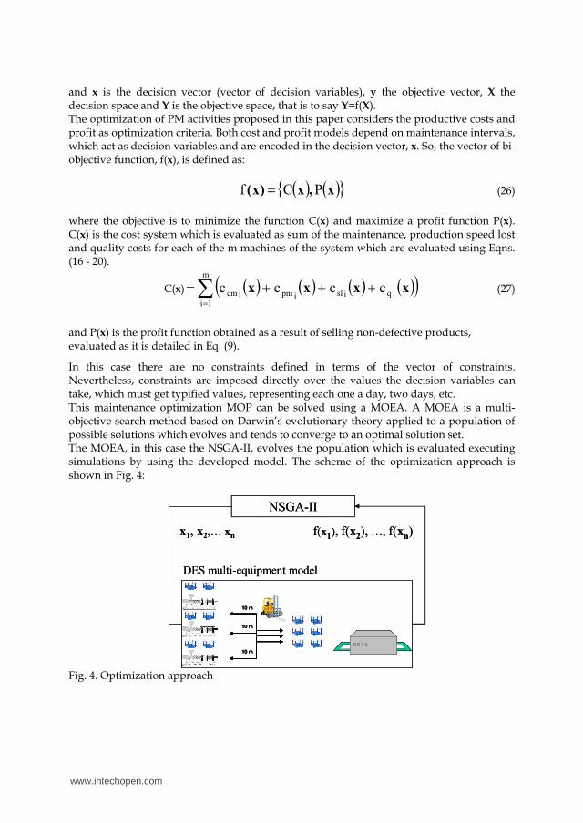
In this case there are no constraints defined in terms of the vector of constraints. Nevertheless, constraints are imposed directly over the values the decision variables can take, which must get typified values, representing each one a day, two days, etc. This maintenance optimization MOP can be solved using a MOEA. A MOEA is a multi-objective search method based on Darwin’s evolutionary theory applied to a population of possible solutions which evolves and tends to converge to an optimal solution set. The MOEA, in this case the NSGA-II, evolves the population which is evaluated executing simulations by using the developed model. The scheme of the optimization approach is shown in Fig. 4:
NSGA-II
x1, x2,… xn f(x1), f(x2), …, f(xn)
10 m
10 m
10 m
10 m
10 m
10 m
DES multi-equipment model
NSGA-II
x1, x2,… xn f(x1), f(x2), …, f(xn)
10 m
10 m
10 m
10 m
10 m
10 m
DES multi-equipment model
Fig. 4. Optimization approach
As it can be seen in Fig. 4, the NSGA-II creates a population of n decision vectors (x1, x2,… xn) which are evaluated executing simulations. The model returns the fitness values of each one of these vectors (f(x1), f(x2), …, f(xn)) which are processed in the NSGA-II to generate new populations. These evolutions tend to achieve solutions which are located in a Pareto optimal front, where it cannot be determined that a solution obtained is better than another without considering additional information.
7. Results
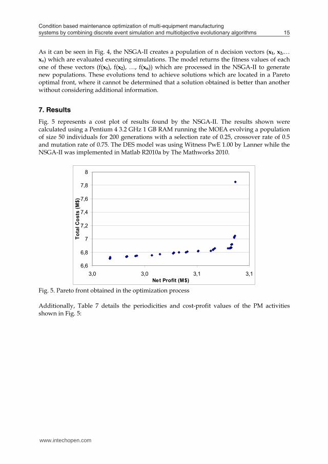
Fig. 5 represents a cost plot of results found by the NSGA-II. The results shown were calculated using a Pentium 4 3.2 GHz 1 GB RAM running the MOEA evolving a population of size 50 individuals for 200 generations with a selection rate of 0.25, crossover rate of 0.5 and mutation rate of 0.75. The DES model was using Witness PwE 1.00 by Lanner while the NSGA-II was implemented in Matlab R2010a by The Mathworks 2010.
6,6
6,8
7
7,2
7,4
7,6
7,8
8
3,0 3,0 3,1 3,1Net Profit (M$)
Tota
l Cos
ts (M
$)
Fig. 5. Pareto front obtained in the optimization process Additionally, Table 7 details the periodicities and cost-profit values of the PM activities shown in Fig. 5:
www.intechopen.com
Condition based maintenance optimization of multi-equipment manufacturing systems by combining discrete event simulation and multiobjective evolutionary algorithms 15
and x is the decision vector (vector of decision variables), y the objective vector, X the decision space and Y is the objective space, that is to say Y=f(X). The optimization of PM activities proposed in this paper considers the productive costs and profit as optimization criteria. Both cost and profit models depend on maintenance intervals, which act as decision variables and are encoded in the decision vector, x. So, the vector of bi-objective function, f(x), is defined as: x,x)x( PCf (26) where the objective is to minimize the function C(x) and maximize a profit function P(x). C(x) is the cost system which is evaluated as sum of the maintenance, production speed lost and quality costs for each of the m machines of the system which are evaluated using Eqns. (16 - 20).
C(x) m
1iiqislipmicm cccc xxxx (27)
and P(x) is the profit function obtained as a result of selling non-defective products, evaluated as it is detailed in Eq. (9).
In this case there are no constraints defined in terms of the vector of constraints. Nevertheless, constraints are imposed directly over the values the decision variables can take, which must get typified values, representing each one a day, two days, etc. This maintenance optimization MOP can be solved using a MOEA. A MOEA is a multi-objective search method based on Darwin’s evolutionary theory applied to a population of possible solutions which evolves and tends to converge to an optimal solution set. The MOEA, in this case the NSGA-II, evolves the population which is evaluated executing simulations by using the developed model. The scheme of the optimization approach is shown in Fig. 4:
NSGA-II
x1, x2,… xn f(x1), f(x2), …, f(xn)
10 m
10 m
10 m
10 m
10 m
10 m
DES multi-equipment model
NSGA-II
x1, x2,… xn f(x1), f(x2), …, f(xn)
10 m
10 m
10 m
10 m
10 m
10 m
DES multi-equipment model
Fig. 4. Optimization approach
As it can be seen in Fig. 4, the NSGA-II creates a population of n decision vectors (x1, x2,… xn) which are evaluated executing simulations. The model returns the fitness values of each one of these vectors (f(x1), f(x2), …, f(xn)) which are processed in the NSGA-II to generate new populations. These evolutions tend to achieve solutions which are located in a Pareto optimal front, where it cannot be determined that a solution obtained is better than another without considering additional information.
7. Results
Fig. 5 represents a cost plot of results found by the NSGA-II. The results shown were calculated using a Pentium 4 3.2 GHz 1 GB RAM running the MOEA evolving a population of size 50 individuals for 200 generations with a selection rate of 0.25, crossover rate of 0.5 and mutation rate of 0.75. The DES model was using Witness PwE 1.00 by Lanner while the NSGA-II was implemented in Matlab R2010a by The Mathworks 2010.
6,6
6,8
7
7,2
7,4
7,6
7,8
8
3,0 3,0 3,1 3,1Net Profit (M$)
Tota
l Cos
ts (M
$)
Fig. 5. Pareto front obtained in the optimization process Additionally, Table 7 details the periodicities and cost-profit values of the PM activities shown in Fig. 5:
www.intechopen.com

Wc1 Wc2 Wc3 Wc4 Wc5 Wc6 Net Profit (€) Total Cost (€)57 24 217 287 101 49 5073840 11569746,08259 203 276 287 36 254 4958660 11391119,09259 220 284 287 36 137 4944400 11376236,31259 234 284 287 36 128 4934460 11363711,18261 21 49 287 36 170 5069720 11557158,79261 21 282 283 36 244 5072660 11558294,87261 24 120 287 36 137 5078500 11824125,91261 24 120 287 36 170 5078700 11819128,42261 24 168 283 36 74 5079760 11864908,78261 24 217 287 36 49 5074500 11577481,48261 24 217 287 36 231 5073900 11570285,34261 24 217 287 36 254 5073840 11569746,08261 24 276 287 36 74 5075560 11658237,44261 24 276 287 36 102 5080300 13330001,56261 24 276 287 36 102 5073260 11551843,41261 24 276 287 36 137 5078820 11839544,71261 24 276 287 57 143 5080480 13209311,2261 24 276 287 36 186 5078780 13088264,73261 24 276 287 36 254 5075040 11644593,44261 24 284 287 36 137 5074240 11575248,3261 24 284 287 36 143 5072840 11561591,77261 72 217 287 36 231 5049060 11529753,47261 72 282 287 36 231 5050680 11557092,2261 74 217 283 36 49 5048160 11520395,78261 77 217 287 36 214 5045100 11494831,02261 88 276 287 36 137 5038940 11503122,02261 104 120 287 36 214 5027520 11491780,06261 107 217 287 36 143 5026920 11484713,39261 128 271 287 57 196 5011400 11474116,47261 129 120 287 36 170 5009660 11458363,92261 143 168 287 36 74 4999720 11453174,76261 156 168 287 36 137 4992060 11442624,64261 156 168 287 36 254 4991260 11423301,86261 156 217 287 36 143 4992340 11441827,68261 156 217 287 36 170 4991340 11429164,3261 182 271 287 36 170 4972380 11407934,91261 182 276 287 36 280 4973340 11402901,84261 199 271 287 36 128 4960780 11378041,99261 229 272 287 36 163 4939140 11369356,24261 231 282 283 36 170 4937080 11361320,55261 249 168 283 36 254 4924000 11340232,17261 249 217 283 36 254 4924860 11351080,1261 249 271 283 36 196 4925160 11354773,53261 249 276 287 36 102 4924580 11339726,48261 249 276 287 36 254 4924500 11337625,08261 249 284 287 36 58 4924680 11343427,54261 282 120 287 36 170 4900260 11297333,11261 282 237 287 36 170 4900680 11305358,67261 282 276 287 36 170 4902120 11337373,85261 282 276 287 36 254 4900700 11306826,13
Table 7. PM periodicities and objective values of the obtained Pareto front
As it was stated previously, the developed MOP offers solutions which are situated in a Pareto optimal front. Thus, the analyst can select externally the best maintenance strategy, since it has to be considered simultaneously possible additional restrictions imposed over the solutions after having them. Hence, they can analyze afterwards how every solution of each Pareto set score in cost and profit criteria. Additionally, the Pareto front generated satisfies the constraint imposed to the problem. Each one of the elements calculated in the Front is related to critical age or deterioration levels when a preventive activity must be executed. So, the decision maker can select a solution of the Pareto front in accordance with his preferences knowing that the elected solution will accomplish all the imposed constraints.
Acknowledgments
We want to thank people of Mondragon Cooperación Cooperativa, for the valuable confidence and help provided to this research. This project has been funded by the following projects and funding programs: DEMAGILE TOOLS: Development of decision making tools for the implementation of principles related to the ‘Leagile production’. Project funded by the Basque Government (Basic and Applied Research Project, PI2009-24 code).
AVAILAFACTURING: Development of a tool for the management of technical assistance service networks for the availability maximization of Manufacturing equipment and/or products (European transnational project MANUNET-2009-BC-006). RCMTOOLS: Development of a simplified RCM tool. Project funded by the Basque Government (University-Industry Research Project, UE2010-03 code).
IMBOEE: Development of a continuous improvement program based on the Money Based OEE. Project funded by the Basque Government (University-Industry Research Project, UE09+/120 code).
8. References Bader, J. M. & Guesneux, S. 2007, "Use real-time optimization for low-sulfur gasoline
production", Hydrocarbon Processing no. February, pp. 97-103. Chan, J. & Shaw, L. 1993, "Modeling repairable systems with failure rates that depend on
age and maintenance", IEEE Transactions on Reliability, vol. 42, no. 4, pp. 566-571. Deb, K., Pratap, A., Agarwal, S., & Meyarivan, T. 2002, "A fast and elitiste multiobjective
genetic algorithm: NSGA-II", IEEE Transactions on Evolutionary Computation, vol. 6, no. 2, pp. 182-197.
Fiori de Castro, H. & Lucchesi Cavalca, K. 2006, "Maintenance resources optimization applied to a manufacturing system", Reliability Engineering and System Safety, vol. 91, pp. 413-420.
Gharbi, A. & Kenné, J. P. 2005, "Maintenance scheduling and production control of multiple-machine manufacturing systems", Computers and Industrial Engineering, vol. 48, pp. 693-702.
www.intechopen.com

Condition based maintenance optimization of multi-equipment manufacturing systems by combining discrete event simulation and multiobjective evolutionary algorithms 17
Wc1 Wc2 Wc3 Wc4 Wc5 Wc6 Net Profit (€) Total Cost (€)57 24 217 287 101 49 5073840 11569746,08259 203 276 287 36 254 4958660 11391119,09259 220 284 287 36 137 4944400 11376236,31259 234 284 287 36 128 4934460 11363711,18261 21 49 287 36 170 5069720 11557158,79261 21 282 283 36 244 5072660 11558294,87261 24 120 287 36 137 5078500 11824125,91261 24 120 287 36 170 5078700 11819128,42261 24 168 283 36 74 5079760 11864908,78261 24 217 287 36 49 5074500 11577481,48261 24 217 287 36 231 5073900 11570285,34261 24 217 287 36 254 5073840 11569746,08261 24 276 287 36 74 5075560 11658237,44261 24 276 287 36 102 5080300 13330001,56261 24 276 287 36 102 5073260 11551843,41261 24 276 287 36 137 5078820 11839544,71261 24 276 287 57 143 5080480 13209311,2261 24 276 287 36 186 5078780 13088264,73261 24 276 287 36 254 5075040 11644593,44261 24 284 287 36 137 5074240 11575248,3261 24 284 287 36 143 5072840 11561591,77261 72 217 287 36 231 5049060 11529753,47261 72 282 287 36 231 5050680 11557092,2261 74 217 283 36 49 5048160 11520395,78261 77 217 287 36 214 5045100 11494831,02261 88 276 287 36 137 5038940 11503122,02261 104 120 287 36 214 5027520 11491780,06261 107 217 287 36 143 5026920 11484713,39261 128 271 287 57 196 5011400 11474116,47261 129 120 287 36 170 5009660 11458363,92261 143 168 287 36 74 4999720 11453174,76261 156 168 287 36 137 4992060 11442624,64261 156 168 287 36 254 4991260 11423301,86261 156 217 287 36 143 4992340 11441827,68261 156 217 287 36 170 4991340 11429164,3261 182 271 287 36 170 4972380 11407934,91261 182 276 287 36 280 4973340 11402901,84261 199 271 287 36 128 4960780 11378041,99261 229 272 287 36 163 4939140 11369356,24261 231 282 283 36 170 4937080 11361320,55261 249 168 283 36 254 4924000 11340232,17261 249 217 283 36 254 4924860 11351080,1261 249 271 283 36 196 4925160 11354773,53261 249 276 287 36 102 4924580 11339726,48261 249 276 287 36 254 4924500 11337625,08261 249 284 287 36 58 4924680 11343427,54261 282 120 287 36 170 4900260 11297333,11261 282 237 287 36 170 4900680 11305358,67261 282 276 287 36 170 4902120 11337373,85261 282 276 287 36 254 4900700 11306826,13
Table 7. PM periodicities and objective values of the obtained Pareto front
As it was stated previously, the developed MOP offers solutions which are situated in a Pareto optimal front. Thus, the analyst can select externally the best maintenance strategy, since it has to be considered simultaneously possible additional restrictions imposed over the solutions after having them. Hence, they can analyze afterwards how every solution of each Pareto set score in cost and profit criteria. Additionally, the Pareto front generated satisfies the constraint imposed to the problem. Each one of the elements calculated in the Front is related to critical age or deterioration levels when a preventive activity must be executed. So, the decision maker can select a solution of the Pareto front in accordance with his preferences knowing that the elected solution will accomplish all the imposed constraints.
Acknowledgments
We want to thank people of Mondragon Cooperación Cooperativa, for the valuable confidence and help provided to this research. This project has been funded by the following projects and funding programs: DEMAGILE TOOLS: Development of decision making tools for the implementation of principles related to the ‘Leagile production’. Project funded by the Basque Government (Basic and Applied Research Project, PI2009-24 code).
AVAILAFACTURING: Development of a tool for the management of technical assistance service networks for the availability maximization of Manufacturing equipment and/or products (European transnational project MANUNET-2009-BC-006). RCMTOOLS: Development of a simplified RCM tool. Project funded by the Basque Government (University-Industry Research Project, UE2010-03 code).
IMBOEE: Development of a continuous improvement program based on the Money Based OEE. Project funded by the Basque Government (University-Industry Research Project, UE09+/120 code).
8. References Bader, J. M. & Guesneux, S. 2007, "Use real-time optimization for low-sulfur gasoline
production", Hydrocarbon Processing no. February, pp. 97-103. Chan, J. & Shaw, L. 1993, "Modeling repairable systems with failure rates that depend on
age and maintenance", IEEE Transactions on Reliability, vol. 42, no. 4, pp. 566-571. Deb, K., Pratap, A., Agarwal, S., & Meyarivan, T. 2002, "A fast and elitiste multiobjective
genetic algorithm: NSGA-II", IEEE Transactions on Evolutionary Computation, vol. 6, no. 2, pp. 182-197.
Fiori de Castro, H. & Lucchesi Cavalca, K. 2006, "Maintenance resources optimization applied to a manufacturing system", Reliability Engineering and System Safety, vol. 91, pp. 413-420.
Gharbi, A. & Kenné, J. P. 2005, "Maintenance scheduling and production control of multiple-machine manufacturing systems", Computers and Industrial Engineering, vol. 48, pp. 693-702.
www.intechopen.com

Goti, A. & Sánchez, A. 2006, "Multi-objective genetic algorithms optimize industrial maintenance", Hydrocarbon Processing, vol. 85, no. 12, pp. 106-108.
Goyal, S. K. & Kusy, M. I. 1985, "Determining economic maintenance frequency for a family of machines", Joumal of the Operations Research Society, vol. 36, no. 12, pp. 1125-1128.
Grigoriev, A., van de Klunder, J., & Spieksma, F. C. R. 2006, "Modeling and solving the periodic maintenance problem", European Journal of Operational Research, vol. 72, pp. 783-797.
Kenne, J. P., Boukas, E. K., & Gharbi, A. 2003, "Control of production and corrective maintenance rates in a multiple-machine, multiple-product manufacturing system", Mathematical and Computer Modelling, vol. 38, pp. 351-365.
Li, W. & Pham, H. 2005, "An inspection-maintenance model for systems with multiple competing processes", IEEE Transactions on Reliability, vol. 54, no. 2, pp. 318-327.
Li, W. & Zuo, M. J. 2007, "Joint Optimization of Inventory Control and Maintenance Policy, in "2007 Proc.Ann.Reliability & Maintainability Symp."", in Reliability and Maintainability in the New Frontier, IEEE, Piscataway, New Jersey, pp. 321-326.
Malik, M. A. K. 1979, "Reliable preventive maintenance scheduling, ", AIIE Transactions, vol. 11, pp. 221-228.
Martorell, S., Sánchez , A., Carlos, S., & Serradell, V. 2004, "Alternatives and challenges in optimizing industrial safety using genetic algorithms", Reliability Engineering and System Safety, vol. 86, no. 1, pp. 25-38.
Martorell, S., Sánchez, A., & Serradell, V. 1998, "Residual life management of safety-related equipment considering maintenance and working conditions", in ESREL'98, Trondheirn, pp. 889-896.
Martorell, S., Sánchez, A., & Serradell, V. 1999, "Age-dependent reliability model considering effects of maintenance and working conditions", Reliability Engineering and Systems Safety, vol. 64, pp. 19-31.
Martorell, S., Serradell, V., & Samanta, P. K. 1995, "Improving allowed outage time and surveillance test interval requirements: a study of their interactions using probabilistic methods", Reliability Engineering and System Safety, vol. 47, no. 2, pp. 119-129.
Oyarbide-Zubillaga, A., Baines, T. S., & Kay, J. M. 2003, "Manufacturing Systems modelling using system dynamics: Forming a dedicated modelling tool", Journal of Advanced Manufacturing Systems, vol. 2, no. 1, pp. 71-87.
Sánchez, A. & Goti, A. 2006, "Preventive maintenance optimization under cost and profit criteria for manufacturing equipment, in "Proceedings of ESREL 2006"", in Proceedings of ESREL 2006: Safety and Reliability for Managing Risk, C. Guedes Soares & E. Zio, eds., Taylor & Francis Group, London, UK, pp. 607-612.
Sherif, Y. S. & Smith, M. L. 1981, "Optimal maintenance models for systems subject to failure", Naval Research Logistics Quarterly, vol. 28, no. 1, pp. 47-74.
Shin, Y., Lim, T. J., & Lie, C. H. 1996, "Estimating parameters of intensity function and maintenance effect for repairable unit", Reliability Engineering and System Safety, vol. 54, pp. 1-10.
Yao, M.-J. 2005, "On determining the optimal maintenance frequency for a family of machines", Journal of the Chinese Institute of Industrial Engineers, vol. 22, no. 3, pp. 199-209.
www.intechopen.com

Discrete Event SimulationsEdited by Aitor Goti
ISBN 978-953-307-115-2Hard cover, 330 pagesPublisher SciyoPublished online 18, August, 2010Published in print edition August, 2010
InTech EuropeUniversity Campus STeP Ri Slavka Krautzeka 83/A 51000 Rijeka, Croatia Phone: +385 (51) 770 447 Fax: +385 (51) 686 166www.intechopen.com
InTech ChinaUnit 405, Office Block, Hotel Equatorial Shanghai No.65, Yan An Road (West), Shanghai, 200040, China
Phone: +86-21-62489820 Fax: +86-21-62489821
Considered by many authors as a technique for modelling stochastic, dynamic and discretely evolvingsystems, this technique has gained widespread acceptance among the practitioners who want to representand improve complex systems. Since DES is a technique applied in incredibly different areas, this book reflectsmany different points of view about DES, thus, all authors describe how it is understood and applied withintheir context of work, providing an extensive understanding of what DES is. It can be said that the name of thebook itself reflects the plurality that these points of view represent. The book embraces a number of topicscovering theory, methods and applications to a wide range of sectors and problem areas that have beencategorised into five groups. As well as the previously explained variety of points of view concerning DES,there is one additional thing to remark about this book: its richness when talking about actual data or actualdata based analysis. When most academic areas are lacking application cases, roughly the half part of thechapters included in this book deal with actual problems or at least are based on actual data. Thus, the editorfirmly believes that this book will be interesting for both beginners and practitioners in the area of DES.
How to referenceIn order to correctly reference this scholarly work, feel free to copy and paste the following:
Aitor Goti and Alvaro Garcia (2010). Condition Based Maintenance Optimization of Multi-EquipmentManufacturing Systems by Combining Discrete Event Simulation and Multiobjective Evolutionary Algorithms,Discrete Event Simulations, Aitor Goti (Ed.), ISBN: 978-953-307-115-2, InTech, Available from:http://www.intechopen.com/books/discrete-event-simulations/condition-based-maintenance-optimization-of-multi-equipment-manufacturing-systems-by-combining-discr

© 2010 The Author(s). Licensee IntechOpen. This chapter is distributedunder the terms of the Creative Commons Attribution-NonCommercial-ShareAlike-3.0 License, which permits use, distribution and reproduction fornon-commercial purposes, provided the original is properly cited andderivative works building on this content are distributed under the samelicense.