con ten ts - pdfs.semanticscholar.org · a hash-based tec hnique for ... mark et bask et analysis...
TRANSCRIPT

Contents
6 Mining Association Rules in Large Databases 5
6.1 Association rule mining . . . . . . . . . . . . . . . . . . . . . . . . . . . . . . . . . . . . . . . . . . . . 5
6.1.1 Market basket analysis: A motivating example for association rule mining . . . . . . . . . . . . 5
6.1.2 Basic concepts . . . . . . . . . . . . . . . . . . . . . . . . . . . . . . . . . . . . . . . . . . . . . 6
6.1.3 Association rule mining: A road map . . . . . . . . . . . . . . . . . . . . . . . . . . . . . . . . . 7
6.2 Mining single-dimensional Boolean association rules from transactional databases . . . . . . . . . . . . 8
6.2.1 The Apriori algorithm: Finding frequent itemsets . . . . . . . . . . . . . . . . . . . . . . . . . . 8
6.2.2 Generating association rules from frequent itemsets . . . . . . . . . . . . . . . . . . . . . . . . . 11
6.2.3 Variations of the Apriori algorithm . . . . . . . . . . . . . . . . . . . . . . . . . . . . . . . . . . 12
6.2.4 Iceberg queries . . . . . . . . . . . . . . . . . . . . . . . . . . . . . . . . . . . . . . . . . . . . . 14
6.3 Mining multilevel association rules from transaction databases . . . . . . . . . . . . . . . . . . . . . . 15
6.3.1 Multilevel association rules . . . . . . . . . . . . . . . . . . . . . . . . . . . . . . . . . . . . . . 15
6.3.2 Approaches to mining multilevel association rules . . . . . . . . . . . . . . . . . . . . . . . . . . 17
6.3.3 Checking for redundant multilevel association rules . . . . . . . . . . . . . . . . . . . . . . . . . 19
6.4 Mining multidimensional association rules from relational databases and data warehouses . . . . . . . 20
6.4.1 Multidimensional association rules . . . . . . . . . . . . . . . . . . . . . . . . . . . . . . . . . . 20
6.4.2 Mining multidimensional association rules using static discretization of quantitative attributes 21
6.4.3 Mining quantitative association rules . . . . . . . . . . . . . . . . . . . . . . . . . . . . . . . . . 22
6.4.4 Mining distance-based association rules . . . . . . . . . . . . . . . . . . . . . . . . . . . . . . . 24
6.5 From association mining to correlation analysis . . . . . . . . . . . . . . . . . . . . . . . . . . . . . . . 25
6.5.1 Strong rules are not necessarily interesting: An example . . . . . . . . . . . . . . . . . . . . . . 25
6.5.2 From association analysis to correlation analysis . . . . . . . . . . . . . . . . . . . . . . . . . . 26
6.6 Constraint-based association mining . . . . . . . . . . . . . . . . . . . . . . . . . . . . . . . . . . . . . 27
6.6.1 Metarule-guided mining of association rules . . . . . . . . . . . . . . . . . . . . . . . . . . . . . 27
6.6.2 Mining guided by additional rule constraints . . . . . . . . . . . . . . . . . . . . . . . . . . . . 28
6.7 Summary . . . . . . . . . . . . . . . . . . . . . . . . . . . . . . . . . . . . . . . . . . . . . . . . . . . . 31
1

2 CONTENTS

List of Figures
6.1 Market basket analysis. . . . . . . . . . . . . . . . . . . . . . . . . . . . . . . . . . . . . . . . . . . . . 6
6.2 Transactional data for an AllElectronics branch. . . . . . . . . . . . . . . . . . . . . . . . . . . . . . . . 9
6.3 Generation of candidate itemsets and frequent itemsets. . . . . . . . . . . . . . . . . . . . . . . . . . . 10
6.4 Generation of candidate 3-itemsets, C3, from L2 using the Apriori property. . . . . . . . . . . . . . . . 10
6.5 The Apriori algorithm for discovering frequent itemsets for mining Boolean association rules. . . . . . 12
6.6 A hash-based technique for generating candidate itemsets. . . . . . . . . . . . . . . . . . . . . . . . . . 13
6.7 Mining by partitioning the data. . . . . . . . . . . . . . . . . . . . . . . . . . . . . . . . . . . . . . . . 13
6.8 A concept hierarchy for AllElectronics computer items. . . . . . . . . . . . . . . . . . . . . . . . . . . . 16
6.9 Multilevel mining with uniform support. . . . . . . . . . . . . . . . . . . . . . . . . . . . . . . . . . . . 17
6.10 Multilevel mining with reduced support. . . . . . . . . . . . . . . . . . . . . . . . . . . . . . . . . . . . 17
6.11 Multilevel mining with reduced support, using level-cross �ltering by a single item. . . . . . . . . . . . 17
6.12 Multilevel mining with reduced support, using level-cross �ltering by a k-itemset. Here, k = 2. . . . . 18
6.13 Multilevel mining with controlled level-cross �ltering by single item . . . . . . . . . . . . . . . . . . . . 19
6.14 Lattice of cuboids, making up a 3-dimensional data cube. Each cuboid represents a di�erent group-by.The base cuboid contains the three predicates, age, income, and buys. . . . . . . . . . . . . . . . . . . 22
6.15 A 2-D grid for tuples representing customers who purchase high resolution TVs . . . . . . . . . . . . . 23
6.16 Binning methods like equi-width and equi-depth do not always capture the semantics of interval data. 24
3

4 LIST OF FIGURES

Chapter 6
Mining Association Rules in Large
Databases
c J. Han and M. Kamber, 2000, DRAFT!! DO NOT COPY!! DO NOT DISTRIBUTE!! January 16, 2000
Association rule mining �nds interesting association or correlation relationships among a large set of data items.With massive amounts of data continuously being collected and stored in databases, many industries are becominginterested in mining association rules from their databases. For example, the discovery of interesting associationrelationships among huge amounts of business transaction records can help catalog design, cross-marketing, loss-leader analysis, and other business decision making processes.
A typical example of association rule mining is market basket analysis. This process analyzes customer buyinghabits by �nding associations between the di�erent items that customers place in their \shopping baskets" (Figure6.1). The discovery of such associations can help retailers develop marketing strategies by gaining insight into whichitems are frequently purchased together by customers. For instance, if customers are buying milk, how likely arethey to also buy bread (and what kind of bread) on the same trip to the supermarket? Such information can lead toincreased sales by helping retailers to do selective marketing and plan their shelf space. For instance, placing milkand bread within close proximity may further encourage the sale of these items together within single visits to thestore.
How can we �nd association rules from large amounts of data, where the data are either transactional or relational?Which association rules are the most interesting? How can we help or guide the mining procedure to discoverinteresting associations? What language constructs are useful in de�ning a data mining query language for associationrule mining? In this chapter, we will delve into each of these questions.
6.1 Association rule mining
Association rule mining searches for interesting relationships among items in a given data set. This section provides anintroduction to association rule mining. We begin in Section 6.1.1 by presenting an example of market basket analysis,the earliest form of association rule mining. The basic concepts of mining associations are given in Section 6.1.2.Section 6.1.3 presents a road map to the di�erent kinds of association rules that can be mined.
6.1.1 Market basket analysis: A motivating example for association rule mining
Suppose, as manager of an AllElectronics branch, you would like to learn more about the buying habits of yourcustomers. Speci�cally, you wonder \Which groups or sets of items are customers likely to purchase on a given trip
to the store?". To answer your question, market basket analysis may be performed on the retail data of customertransactions at your store. The results may be used to plan marketing or advertising strategies, as well as catalogdesign. For instance, market basket analysis may help managers design di�erent store layouts. In one strategy, itemsthat are frequently purchased together can be placed in close proximity in order to further encourage the sale of suchitems together. If customers who purchase computers also tend to buy �nancial management software at the sametime, then placing the hardware display close to the software display may help to increase the sales of both of these
5

6 CHAPTER 6. MINING ASSOCIATION RULES IN LARGE DATABASES
Market analyst
milk
bread
cereal milk
bread
breadbutter
milksugar
eggs
sugar eggs
Customer 1 Customer 2 Customer 3
...
...
Hmmm, which items are frequently
purchased together by my customers?
Customer n
SHOPPING BASKETS
Market analyst
milk
bread
cereal milk
bread
breadbutter
milksugar
eggs
sugar eggs
Customer 2 Customer 3
...
...
Hmmm, which items are frequently
purchased together by my customers?
Customer n
SHOPPING BASKETS
Customer 1
Figure 6.1: Market basket analysis.
items. In an alternative strategy, placing hardware and software at opposite ends of the store may entice customerswho purchase such items to pick up other items along the way. For instance, after deciding on an expensive computer,a customer may observe security systems for sale while heading towards the software display to purchase �nancialmanagement software, and may decide to purchase a home security system as well. Market basket analysis can alsohelp retailers to plan which items to put on sale at reduced prices. If customers tend to purchase computers andprinters together, then having a sale on printers may encourage the sale of printers as well as computers.
If we think of the universe as the set of items available at the store, then each item has a Boolean variablerepresenting the presence or absence of that item. Each basket can then be represented by a Boolean vector of valuesassigned to these variable. The Boolean vectors can be analyzed for buying patterns which re ect items that arefrequent associated or purchased together. These patterns can be represented in the form of association rules. Forexample, the information that customers who purchase computers also tend to buy �nancial management softwareat the same time is represented in association Rule (6.1) below.
computer ) �nancial management software [support = 2%; confidence = 60%] (6.1)
Rule support and con�dence are two measures of rule interestingness that were described earlier in Section 1.5.They respectively re ect the usefulness and certainty of discovered rules. A support of 2% for association Rule (6.1)means that 2% of all the transactions under analysis show that computer and �nancial management software arepurchased together. A con�dence of 60%means that 60% of the customers who purchased a computer also bought thesoftware. Typically, association rules are considered interesting if they satisfy both aminimum support threshold
and a minimum con�dence threshold. Such thresholds can be set by users or domain experts.
6.1.2 Basic concepts
Let I=fi1, i2, :::, img be a set of items. Let D, the task relevant data, be a set of database transactions where eachtransaction T is a set of items such that T � I. Each transaction is associated with an identi�er, called TID. Let Abe a set of items. A transaction T is said to contain A if and only if A � T . An association rule is an implicationof the form A ) B, where A � I, B � I and A \ B = �. The rule A ) B holds in the transaction set D withsupport s, where s is the percentage of transactions in D that contain A[B. The rule A ) B has con�dence c

6.1. ASSOCIATION RULE MINING 7
in the transaction set D if c is the percentage of transactions in D containing A which also contain B. That is,
support(A ) B) = P (A [B) (6.2)
confidence(A ) B) = P (BjA): (6.3)
Rules that satisfy both a minimum support threshold (min sup) and a minimum con�dence threshold (min conf) arecalled strong. By convention, we write min sup and min conf values so as to occur between 0% and 100%, ratherthan 0 to 1.0.
A set of items is referred to as an itemset. An itemset that contains k items is a k-itemset. The set fcomputer,�nancial management softwareg is a 2-itemset. The occurrence frequency of an itemset is the number oftransactions that contain the itemset. This is also known, simply, as the frequency or support count of theitemset. An itemset satis�es minimum support if the occurrence frequency of the itemset is greater than or equalto the product of min sup and the total number of transactions in D. The number of transactions required for theitemset to satisfy minimum support is therefore referred to as the minimum support count. If an itemset satis�esminimum support, then it is a frequent itemset1. The set of frequent k-itemsets is commonly denoted by Lk
2.
\How are association rules mined from large databases?" Association rule mining is a two-step process:
� Step 1: Find all frequent itemsets. By de�nition, each of these itemsets will occur at least as frequently as apre-determined minimum support count.
� Step 2: Generate strong association rules from the frequent itemsets. By de�nition, these rules must satisfyminimum support and minimum con�dence.
Additional interestingness measures can be applied, if desired. The second step is the easiest of the two. The overallperformance of mining association rules is determined by the �rst step.
6.1.3 Association rule mining: A road map
Market basket analysis is just one form of association rule mining. In fact, there are many kinds of association rules.Association rules can be classi�ed in various ways, based on the following criteria:
1. Based on the types of values handled in the rule:
If a rule concerns associations between the presence or absence of items, it is a Boolean association rule.For example, Rule (6.1) above is a Boolean association rule obtained from market basket analysis.
If a rule describes associations between quantitative items or attributes, then it is a quantitative associationrule. In these rules, quantitative values for items or attributes are partitioned into intervals. Rule (6.4) belowis an example of a quantitative association rule.
age(X; \30� 34") ^ income(X; \42K � 48K") ) buys(X ; \high resolution TV ") (6.4)
Note that the quantitative attributes, age and income, have been discretized.
2. Based on the dimensions of data involved in the rule:
If the items or attributes in an association rule each reference only one dimension, then it is a single-
dimensional association rule. Note that Rule (6.1) could be rewritten as
buys(X ; \computer")) buys(X ; \�nancial management software") (6.5)
Rule (6.1) is therefore a single-dimensional association rule since it refers to only one dimension, i.e., buys.
If a rule references two or more dimensions, such as the dimensions buys, time of transaction, and cus-
tomer category, then it is a multidimensional association rule. Rule (6.4) above is considered a multi-dimensional association rule since it involves three dimensions, age, income, and buys.
1In early work, itemsets satisfying minimum support were referred to as large. This term, however, is somewhat confusing as it hasconnotations to the number of items in an itemset rather than the frequency of occurrence of the set. Hence, we use the more recentterm of frequent.
2Although the term frequent is preferred over large, for historical reasons frequent k-itemsets are still denoted as Lk.

8 CHAPTER 6. MINING ASSOCIATION RULES IN LARGE DATABASES
3. Based on the levels of abstractions involved in the rule set:
Some methods for association rule mining can �nd rules at di�ering levels of abstraction. For example, supposethat a set of association rules mined included Rule (6.6) and (6.7) below.
age(X; \30� 34")) buys(X ; \laptop computer") (6.6)
age(X; \30� 34")) buys(X ; \computer") (6.7)
In Rules (6.6) and (6.7), the items bought are referenced at di�erent levels of abstraction. (That is, \computer"is a higher level abstraction of \laptop computer"). We refer to the rule set mined as consisting of multilevelassociation rules. If, instead, the rules within a given set do not reference items or attributes at di�erentlevels of abstraction, then the set contains single-level association rules.
4. Based on the nature of the association involved in the rule: Association mining can be extended to correlationanalysis, where the absence or presence of correlated items can be identi�ed.
Throughout the rest of this chapter, you will study methods for mining each of the association rule types described.
6.2 Mining single-dimensional Boolean association rules from transactional databases
In this section, you will learn methods for mining the simplest form of association rules - single-dimensional, single-level, Boolean association rules, such as those discussed for market basket analysis in Section 6.1.1. We begin bypresenting Apriori, a basic algorithm for �nding frequent itemsets (Section 6.2.1). A procedure for generating strongassociation rules from frequent itemsets is discussed in Section 6.2.2. Section 6.2.3 describes several variations to theApriori algorithm for improved e�ciency and scalability.
6.2.1 The Apriori algorithm: Finding frequent itemsets
Apriori is an in uential algorithm for mining frequent itemsets for Boolean association rules. The name of thealgorithm is based on the fact that the algorithm uses prior knowledge of frequent itemset properties, as we shallsee below. Apriori employs an iterative approach known as a level-wise search, where k-itemsets are used to explore(k+1)-itemsets. First, the set of frequent 1-itemsets is found. This set is denoted L1. L1 is used to �nd L2, thefrequent 2-itemsets, which is used to �nd L3, and so on, until no more frequent k-itemsets can be found. The �ndingof each Lk requires one full scan of the database.
To improve the e�ciency of the level-wise generation of frequent itemsets, an important property called the
Apriori property, presented below, is used to reduce the search space. We will �rst describe this property, and thenshow an example illustrating its use.
The Apriori property. All non-empty subsets of a frequent itemset must also be frequent.
This property is based on the following observation. By de�nition, if an itemset I does not satisfy the minimumsupport threshold, s, then I is not frequent, i.e., P (I) < s. If an item A is added to the itemset I, then the resultingitemset (i.e., I [A) cannot occur more frequently than I. Therefore, I [A is not frequent either, i.e., P (I [A) < s.
This property belongs to a special category of properties called anti-monotone in the sense that if a set cannot
pass a test, all of its supersets will fail the same test as well. It is called anti-monotone because the property ismonotonic in the context of failing a test.
\How is the Apriori property used in the algorithm?" To understand this, we must look at how Lk�1 is used to�nd Lk. A two step process is followed, consisting of join and prune actions.
6.2. MINING SINGLE-DIMENSIONAL BOOLEAN ASSOCIATION RULES FROMTRANSACTIONAL DATABASES9
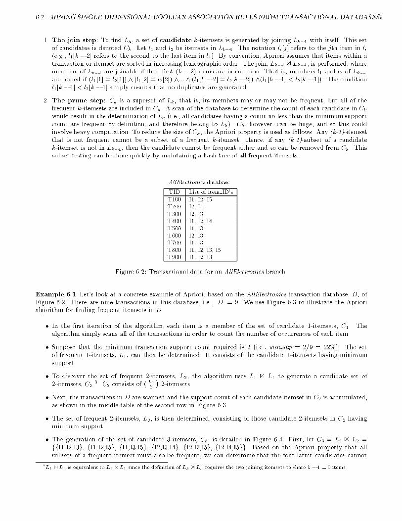
1. The join step: To �nd Lk, a set of candidate k-itemsets is generated by joining Lk�1 with itself. This setof candidates is denoted Ck. Let l1 and l2 be itemsets in Lk�1. The notation li[j] refers to the jth item in li(e.g., l1[k � 2] refers to the second to the last item in l1). By convention, Apriori assumes that items within atransaction or itemset are sorted in increasing lexicographic order. The join, Lk�1 1 Lk�1, is performed, wheremembers of Lk�1 are joinable if their �rst (k � 2) items are in common. That is, members l1 and l2 of Lk�1
are joined if (l1[1] = l2[1]) ^ (l1[2] = l2[2]) ^::: ^ (l1[k � 2] = l2[k � 2]) ^(l1[k � 1] < l2[k � 1]). The conditionl1[k � 1] < l2[k � 1] simply ensures that no duplicates are generated.
2. The prune step: Ck is a superset of Lk, that is, its members may or may not be frequent, but all of thefrequent k-itemsets are included in Ck. A scan of the database to determine the count of each candidate in Ck
would result in the determination of Lk (i.e., all candidates having a count no less than the minimum supportcount are frequent by de�nition, and therefore belong to Lk). Ck, however, can be huge, and so this couldinvolve heavy computation. To reduce the size of Ck, the Apriori property is used as follows. Any (k-1)-itemsetthat is not frequent cannot be a subset of a frequent k-itemset. Hence, if any (k-1)-subset of a candidatek-itemset is not in Lk�1, then the candidate cannot be frequent either and so can be removed from Ck. Thissubset testing can be done quickly by maintaining a hash tree of all frequent itemsets.
AllElectronics database
TID List of item ID's
T100 I1, I2, I5
T200 I2, I4
T300 I2, I3T400 I1, I2, I4
T500 I1, I3
T600 I2, I3
T700 I1, I3
T800 I1, I2, I3, I5
T900 I1, I2, I3
Figure 6.2: Transactional data for an AllElectronics branch.
Example 6.1 Let's look at a concrete example of Apriori, based on the AllElectronics transaction database, D, ofFigure 6.2. There are nine transactions in this database, i.e., jDj = 9. We use Figure 6.3 to illustrate the Apriorialgorithm for �nding frequent itemsets in D.
� In the �rst iteration of the algorithm, each item is a member of the set of candidate 1-itemsets, C1. Thealgorithm simply scans all of the transactions in order to count the number of occurrences of each item.
� Suppose that the minimum transaction support count required is 2 (i.e., min sup = 2=9 = 22%). The setof frequent 1-itemsets, L1, can then be determined. It consists of the candidate 1-itemsets having minimumsupport.
� To discover the set of frequent 2-itemsets, L2, the algorithm uses L1 1 L1 to generate a candidate set of2-itemsets, C2
3. C2 consists of�jL1j
2
�2-itemsets.
� Next, the transactions in D are scanned and the support count of each candidate itemset in C2 is accumulated,as shown in the middle table of the second row in Figure 6.3.
� The set of frequent 2-itemsets, L2, is then determined, consisting of those candidate 2-itemsets in C2 havingminimum support.
� The generation of the set of candidate 3-itemsets, C3, is detailed in Figure 6.4. First, let C3 = L2 1 L2 =ffI1,I2,I3g, fI1,I2,I5g, fI1,I3,I5g, fI2,I3,I4g, fI2,I3,I5g, fI2,I4,I5gg. Based on the Apriori property that allsubsets of a frequent itemset must also be frequent, we can determine that the four latter candidates cannot
3L1 1 L1 is equivalent to L1 � L1 since the de�nition of L
k1 L
krequires the two joining itemsets to share k � 1 = 0 items.

10 CHAPTER 6. MINING ASSOCIATION RULES IN LARGE DATABASES
Scan D for
count of eachcandidate
�!
C1
Itemset Sup.
fI1g 6
fI2g 7
fI3g 6fI4g 2
fI5g 2
Compare candidate
support withminimum support
count
�!
L1
Itemset Sup.
fI1g 6
fI2g 7fI3g 6
fI4g 2
fI5g 2
Generate C2
candidates fromL1
�!
C2
Itemset
fI1,I2g
fI1,I3gfI1,I4g
fI1,I5g
fI2,I3g
fI2,I4g
fI2,I5gfI3,I4g
fI3,I5g
fI4,I5g
Scan D for
count ofeach candidate
�!
C2
Itemset Sup.
fI1,I2g 4
fI1,I3g 4fI1,I4g 1
fI1,I5g 2
fI2,I3g 4fI2,I4g 2
fI2,I5g 2
fI3,I4g 0fI3,I5g 1
fI4,I5g 0
Compare candidate
support withminimum support
count
�!
L2
Itemset Sup.
fI1,I2g 4
fI1,I3g 4fI1,I5g 2
fI2,I3g 4
fI2,I4g 2
fI2,I5g 2
Generate C3
candidates fromL2
�!
C3
Itemset
fI1,I2,I3g
fI1,I2,I5g
Scan D for
count of eachcandidate
�!
C3
Itemset Sup.
fI1,I2,I3g 2
fI1,I2,I5g 2
Compare candidatesupport with
minimum support
count�!
L3
Itemset Sup.
fI1,I2,I3g 2
fI1,I2,I5g 2
Figure 6.3: Generation of candidate itemsets and frequent itemsets, where the minimum support count is 2.
1. Join: C3 = L2 1 L2 = ffI1,I2g, ffI1,I3g, ffI1,I5g, fI2,I3g, fI2,I4g, fI2,I5gg 1 ffI1,I2g, ffI1,I3g, ffI1,I5g,fI2,I3g, fI2,I4g, fI2,I5gg = ffI1,I2,I3g, fI1,I2,I5g, fI1,I3,I5g, fI2,I3,I4g, fI2,I3,I5g, fI2,I4,I5gg.
2. Prune using the Apriori property: All subsets of a frequent itemset must also be frequent. Do any of thecandidates have a subset that is not frequent?
{ The 2-item subsets of fI1,I2,I3g are fI1,I2g, fI1,I3g, and fI2,I3g. All 2-item subsets of fI1,I2,I3g aremembers of L2. Therefore, keep fI1,I2,I3g in C3.
{ The 2-item subsets of fI1,I2,I5g are fI1,I2g, fI1,I5g, and fI2,I5g. All 2-item subsets of fI1,I2,I5g aremembers of L2. Therefore, keep fI1,I2,I5g in C3.
{ The 2-item subsets of fI1,I3,I5g are fI1,I3g, fI1,I5g, and fI3,I5g. fI3,I5g is not a member of L2, and soit is not frequent. Therefore, remove fI1,I3,I5g from C3.
{ The 2-item subsets of fI2,I3,I4g are fI2,I3g, fI2,I4g, and fI3,I4g. fI3,I4g is not a member of L2, and soit is not frequent. Therefore, remove fI2,I3,I4g from C3.
{ The 2-item subsets of fI2,I3,I5g are fI2,I3g, fI2,I5g, and fI3,I5g. fI3,I5g is not a member of L2, and soit is not frequent. Therefore, remove fI2,I3,I5g from C3.
{ The 2-item subsets of fI2,I4,I5g are fI2,I4g, fI2,I5g, and fI4,I5g. fI4,I5g is not a member of L2, and soit is not frequent. Therefore, remove fI2,I4,I5g from C3.
3. Therefore, C3 = ffI1,I2,I3g, fI1,I2,I5gg after pruning.
Figure 6.4: Generation of candidate 3-itemsets, C3, from L2 using the Apriori property.

6.2. MINING SINGLE-DIMENSIONAL BOOLEAN ASSOCIATION RULES FROMTRANSACTIONAL DATABASES11
possibly be frequent. We therefore remove them from C3, thereby saving the e�ort of unnecessarily obtainingtheir counts during the subsequent scan of D to determine L3. Note that when given a candidate k-itemset, weonly need to check if its (k-1)-subsets are frequent since the Apriori algorithm uses a level-wise search strategy.
� The transactions in D are scanned in order to determine L3, consisting of those candidate 3-itemsets in C3
having minimum support (Figure 6.3).
� The algorithm uses L3 1 L3 to generate a candidate set of 4-itemsets, C4. Although the join results inffI1; I2; I3; I5gg, this itemset is pruned since its subset ffI2; I3; I5gg is not frequent. Thus, C4 = �, and thealgorithm terminates, having found all of the frequent itemsets.
2
Figure 6.5 shows pseudo-code for the Apriori algorithm and its related procedures. Step 1 of Apriori �nds thefrequent 1-itemsets, L1. In steps 2-10, Lk�1 is used to generate candidates Ck in order to �nd Lk. The apriori genprocedure generates the candidates and then uses the Apriori property to eliminate those having a subset that isnot frequent (step 3). This procedure is described below. Once all the candidates have been generated, the databaseis scanned (step 4). For each transaction, a subset function is used to �nd all subsets of the transaction thatare candidates (step 5), and the count for each of these candidates is accumulated (steps 6-7). Finally, all thosecandidates satisfying minimum support form the set of frequent itemsets, L. A procedure can then be called togenerate association rules from the frequent itemsets. Such as procedure is described in Section 6.2.2.
The apriori gen procedure performs two kinds of actions, namely join and prune, as described above. In the joincomponent, Lk�1 is joined with Lk�1 to generate potential candidates (steps 1-4). The prune component (steps 5-7)employs the Apriori property to remove candidates that have a subset that is not frequent. The test for infrequentsubsets is shown in procedure has infrequent subset.
6.2.2 Generating association rules from frequent itemsets
Once the frequent itemsets from transactions in a database D have been found, it is straightforward to generatestrong association rules from them (where strong association rules satisfy both minimum support and minimumcon�dence). This can be done using Equation (6.8) for con�dence, where the conditional probability is expressedin terms of itemset support count:
confidence(A ) B) = P (BjA) =support count(A [B)
support count(A); (6.8)
where support count(A [B) is the number of transactions containing the itemsets A [B, and support count(A) isthe number of transactions containing the itemset A. Based on this equation, association rules can be generated asfollows.
� For each frequent itemset, l, generate all non-empty subsets of l.
� For every non-empty subset s, of l, output the rule \s) (l� s)" ifsupport count(l)
support count(s)� min conf, where min conf
is the minimum con�dence threshold.
Since the rules are generated from frequent itemsets, then each one automatically satis�es minimum support. Fre-quent itemsets can be stored ahead of time in hash tables along with their counts so that they can be accessedquickly.
Example 6.2 Let's try an example based on the transactional data for AllElectronics shown in Figure 6.2. Supposethe data contains the frequent itemset l = fI1,I2,I5g. What are the association rules that can be generated from l?The non-empty subsets of l are fI1,I2g, fI1,I5g, fI2,I5g, fI1g, fI2g, and fI5g. The resulting association rules are asshown below, each listed with its con�dence.
I1 ^ I2) I5, con�dence= 2=4 = 50%I1 ^ I5) I2, con�dence= 2=2 = 100%

12 CHAPTER 6. MINING ASSOCIATION RULES IN LARGE DATABASES
Algorithm 6.2.1 (Apriori) Find frequent itemsets using an iterative level-wise approach.
Input: Database, D, of transactions; minimum support threshold, min sup.
Output: L, frequent itemsets in D.
Method:
1) L1 = �nd frequent 1-itemsets(D);
2) for (k = 2;Lk�1 6= �;k++) f
3) Ck = apriori gen(Lk�1, min sup);4) for each transaction t 2 D f // scan D for counts
5) Ct = subset(Ck ; t); // get the subsets of t that are candidates6) for each candidate c 2 Ct
7) c.count++;
8) g
9) Lk = fc 2 Ck jc:count� min supg10) g
11) return L = [kLk;
procedure apriori gen(Lk�1:frequent (k-1)-itemsets; min sup: minimum support)
1) for each itemset l1 2 Lk�12) for each itemset l2 2 Lk�1
3) if (l1[1] = l2[1]) ^ (l1[2] = l2[2]) ^ :::^ (l1[k� 2] = l2[k� 2]) ^ (l1[k � 1] < l2[k� 1]) then f
4) c = l1 1 l2; // join step: generate candidates5) if has infrequent subset(c;Lk�1) then
6) delete c; // prune step: remove unfruitful candidate
7) else add c to Ck;8) g
9) return Ck;
procedure has infrequent subset(c: candidate k-itemset; Lk�1: frequent (k� 1)-itemsets); // use prior knowledge
1) for each (k � 1)-subset s of c
2) if s 62 Lk�1 then
3) return TRUE;
4) return FALSE;
Figure 6.5: The Apriori algorithm for discovering frequent itemsets for mining Boolean association rules.
I2 ^ I5) I1, con�dence= 2=2 = 100%I1) I2 ^ I5, con�dence= 2=6 = 33%I2) I1 ^ I5, con�dence= 2=7 = 29%I5) I1 ^ I2, con�dence= 2=2 = 100%
If the minimum con�dence threshold is, say, 70%, then only the second, third, and last rules above are output, sincethese are the only ones generated that are strong. 2
6.2.3 Variations of the Apriori algorithm
\How might the e�ciency of Apriori be improved?"
Many variations of the Apriori algorithm have been proposed. A number of these variations are enumeratedbelow. Methods 1 to 6 focus on improving the e�ciency of the original algorithm, while methods 7 and 8 considertransactions over time.
1. A hash-based technique: Hashing itemset counts.
A hash-based technique can be used to reduce the size of the candidate k-itemsets, Ck, for k > 1. For example,when scanning each transaction in the database to generate the frequent 1-itemsets, L1, from the candidate

6.2. MINING SINGLE-DIMENSIONAL BOOLEAN ASSOCIATION RULES FROMTRANSACTIONAL DATABASES13
Create hash table, H2
using hash functionh(x; y) = ((order of x) � 10
+(order of y)) mod 7
�!
H2
bucket address 0 1 2 3 4 5 6
bucket count 2 2 4 2 2 4 4
bucket contents fI1,I4g fI1,I5g fI2,I3g fI2,I4g fI2,I5g fI1,I2g fI1,I3g
fI3,I5g fI1,I5g fI2,I3g fI2,I4g fI2,I5g fI1,I2g fI1,I3g
fI2,I3g fI1,I2g fI1,I3g
fI2,I3g fI1,I2g fI1,I3g
Figure 6.6: Hash table, H2, for candidate 2-itemsets: This hash table was generated by scanning the transactions ofFigure 6.2 while determining L1 from C1. If the minimum support count is, say, 3, then the itemsets in buckets 0,1, 3, and 4 cannot be frequent and so they should not be included in C2.
1-itemsets in C1, we can generate all of the 2-itemsets for each transaction, hash (i.e., map) them into thedi�erent buckets of a hash table structure, and increase the corresponding bucket counts (Figure 6.6). A 2-itemset whose corresponding bucket count in the hash table is below the support threshold cannot be frequentand thus should be removed from the candidate set. Such a hash-based technique may substantially reducethe number of the candidate k-itemsets examined (especially when k = 2).
2. Transaction reduction: Reducing the number of transactions scanned in future iterations.
A transaction which does not contain any frequent k-itemsets cannot contain any frequent (k + 1)-itemsets.Therefore, such a transaction can be marked or removed from further consideration since subsequent scans ofthe database for j-itemsets, where j > k, will not require it.
3. Partitioning: Partitioning the data to �nd candidate itemsets.
A partitioning technique can be used which requires just two database scans to mine the frequent itemsets(Figure 6.7). It consists of two phases. In Phase I, the algorithm subdivides the transactions of D into n
non-overlapping partitions. If the minimum support threshold for transactions in D is min sup, then theminimum itemset support count for a partition is min sup � the number of transactions in that partition. Foreach partition, all frequent itemsets within the partition are found. These are referred to as local frequentitemsets. The procedure employs a special data structure which, for each itemset, records the TID's of thetransactions containing the items in the itemset. This allows it to �nd all of the local frequent k-itemsets, fork = 1; 2; : : :, in just one scan of the database.
A local frequent itemset may or may not be frequent with respect to the entire database, D. Any itemset
that is potentially frequent with respect to D must occur as a frequent itemset in at least one of the partitions.Therefore, all local frequent itemsets are candidate itemsets with respect to D. The collection of frequentitemsets from all partitions forms a global candidate itemset with respect to D. In Phase II, a second scanof D is conducted in which the actual support of each candidate is assessed in order to determine the globalfrequent itemsets. Partition size and the number of partitions are set so that each partition can �t into mainmemory and therefore be read only once in each phase.
Divided D into
n partitions
Find global
frequent itemsets
among candidates
(1 scan)
Find the frequent
itemsets local to
each partition
(1 scan)
Frequent
itemsets in Din D
Transactions
PHASE I PHASE II
local frequent
candidate itemset
itemsets to form
Combine all
Figure 6.7: Mining by partitioning the data.

14 CHAPTER 6. MINING ASSOCIATION RULES IN LARGE DATABASES
4. Sampling: Mining on a subset of the given data.
The basic idea of the sampling approach is to pick a random sample S of the given data D, and then searchfor frequent itemsets in S instead D. In this way, we trade o� some degree of accuracy against e�ciency. Thesample size of S is such that the search for frequent itemsets in S can be done in main memory, and so, onlyone scan of the transactions in S is required overall. Because we are searching for frequent itemsets in S ratherthan in D, it is possible that we will miss some of the global frequent itemsets. To lessen this possibility, weuse a lower support threshold than minimum support to �nd the frequent itemsets local to S (denoted LS ).The rest of the database is then used to compute the actual frequencies of each itemset in LS . A mechanismis used to determine whether all of the global frequent itemsets are included in LS . If LS actually containedall of the frequent itemsets in D, then only one scan of D was required. Otherwise, a second pass can be donein order to �nd the frequent itemsets that were missed in the �rst pass. The sampling approach is especiallybene�cial when e�ciency is of utmost importance, such as in computationally intensive applications that mustbe run on a very frequent basis.
5. Dynamic itemset counting: Adding candidate itemsets at di�erent points during a scan.
A dynamic itemset counting technique was proposed in which the database is partitioned into blocks marked bystart points. In this variation, new candidate itemsets can be added at any start point, unlike in Apriori, whichdetermines new candidate itemsets only immediately prior to each complete database scan. The techniqueis dynamic in that it estimates the support of all of the itemsets that have been counted so far, adding newcandidate itemsets if all of their subsets are estimated to be frequent. The resulting algorithm requires twodatabase scans.
6. Calendric market basket analysis: Finding itemsets that are frequent in a set of user-de�ned time intervals.
Calendric market basket analysis uses transaction time stamps to de�ne subsets of the given database. Thesesubsets are considered \calendars" where a calendar is any group of dates such as \every �rst of the month",or \every Thursday in the year 1999". Association rules are formed for itemsets that occur for every day inthe calendar. In this way, an itemset that would not otherwise satisfy minimum support may be consideredfrequent with respect to a subset of the database which satis�es the calendric time constraints.
7. Sequential patterns: Finding sequences of transactions associated over time.
The goal of sequential pattern analysis is to �nd sequences of itemsets that many customers have purchased inroughly the same order. A transaction sequence is said to contain an itemset sequence if each itemset iscontained in one transaction, and the following condition is satis�ed: If the ith itemset in the itemset sequenceis contained in transaction j in the transaction sequence, then the (i + 1)th itemset in the itemset sequence iscontained in a transaction numbered greater than j. The support of an itemset sequence is the percentage oftransaction sequences that contain it.
Other variations involving the mining of multilevel and multidimensional association rules are discussed in therest of this chapter. The mining of time sequences is further discussed in Chapter 9.
6.2.4 Iceberg queries
The Apriori algorithm can be used to improve the e�ciency of answering iceberg queries. Iceberg queries arecommonly used in data mining, particularly for market basket analysis. An iceberg query computes an aggregatefunction over an attribute or set of attributes in order to �nd aggregate values above some speci�ed threshold. Givena relation R with attributes a 1; a 2; :::; a n and b, and an aggregate function, agg f, an iceberg query is of the form
select R.a 1, R.a 2, ..., R.a n, agg f(R.b)from relation Rgroup by R.a 1, R.a 2, ..., R.a nhaving agg f(R.b) >= threshold
Given the large amount of input data tuples, the number of tuples that will satisfy the threshold in the having clauseis relatively small. The output result is seen as the \tip of the iceberg", where the \iceberg" is the set of input data.

6.3. MINING MULTILEVEL ASSOCIATION RULES FROM TRANSACTION DATABASES 15
Example 6.3 An iceberg query. Suppose that, given sales data, you would like to generate a list of customer-item pairs for customers who have purchased items in a quantity of three or more. This can be expressed with thefollowing iceberg query.
select P.cust ID, P.item ID, SUM(P.qty)from Purchases Pgroup by P.cust ID, P.item IDhaving SUM(P.qty) >= 3
2
\How can the query of Example 6.3 be answered?", you ask. A common strategy is to apply hashing or sorting tocompute the value of the aggregate function, SUM, for all of the customer-item groups, and then remove those forwhich the quantity of items purchased by the given customer was less than three. The number of tuples satisfying thiscondition is likely to be small with respect to the total number of tuples processed, leaving room for improvementsin e�ciency. Alternatively, we can use a variation of the Apriori property to prune the number of customer-itempairs considered. That is, instead of looking at the quantities of each item purchased by each customer, we can dothe following:
� Generate cust list, a list of customers who bought three or more items in total, e.g.,
select P.cust IDfrom Purchases Pgroup by P.cust IDhaving SUM(P.qty) >= 3
� Generate item list, a list of items that were purchased by any customer in quantities of three or more, e.g.,
select P.item IDfrom Purchases Pgroup by P.item IDhaving SUM(P.qty) >= 3
From this a priori knowledge, we can eliminate many of the customer-item pairs that would otherwise have beengenerated in the hashing/sorting approach: only generate candidate customer-item pairs for customers in cust list
and items in item list. A count is maintained for such pairs. While the approach improves e�ciency by pruningmany pairs or groups a priori, the resulting number of customer-item pairs may still be so large that it does not �tinto main memory. Hashing and sampling strategies may be integrated into the process to help improve the overalle�ciency of this query answering technique.
6.3 Mining multilevel association rules from transaction databases
6.3.1 Multilevel association rules
For many applications, it is di�cult to �nd strong associations among data items at low or primitive levels ofabstraction due to the sparsity of data in multidimensional space. Strong associations discovered at very highconcept levels may represent common sense knowledge. However, what may represent common sense to one user,may seem novel to another. Therefore, data mining systems should provide capabilities to mine association rules atmultiple levels of abstraction and traverse easily among di�erent abstraction spaces.
Let's examine the following example.
Example 6.4 Suppose we are given the task-relevant set of transactional data in Table 6.1 for sales at the computerdepartment of an AllElectronics branch, showing the items purchased for each transaction TID. The concept hierarchyfor the items is shown in Figure 6.8. A concept hierarchy de�nes a sequence of mappings from a set of low levelconcepts to higher level, more general concepts. Data can be generalized by replacing low level concepts within the

16 CHAPTER 6. MINING ASSOCIATION RULES IN LARGE DATABASES
financial
management
accessory
computer
wrist
pad
Ergo-
way
mouse
Logitech
software
educationalhome laptop color b/w
printer
IBM Microsoft HP Canon
computer
Epson
all(computer items)
Figure 6.8: A concept hierarchy for AllElectronics computer items.
data by their higher level concepts, or ancestors, from a concept hierarchy 4. The concept hierarchy of Figure 6.8 hasfour levels, referred to as levels 0, 1, 2, and 3. By convention, levels within a concept hierarchy are numbered from topto bottom, starting with level 0 at the root node for all (the most general abstraction level). Here, level 1 includescomputer, software, printer and computer accessory, level 2 includes home computer, laptop computer, educationsoftware, �nancial management software, .., and level 3 includes IBM home computer, .., Microsoft educational
software, and so on. Level 3 represents the most speci�c abstraction level of this hierarchy. Concept hierarchies maybe speci�ed by users familiar with the data, or may exist implicitly in the data.
TID Items Purchased
1 IBM home computer, Sony b/w printer2 Microsoft educational software, Microsoft �nancial management software3 Logitech mouse computer-accessory, Ergo-way wrist pad computer-accessory4 IBM home computer, Microsoft �nancial management software5 IBM home computer. . . . . .
Table 6.1: Task-relevant data, D.
The items in Table 6.1 are at the lowest level of the concept hierarchy of Figure 6.8. It is di�cult to �nd interestingpurchase patterns at such raw or primitive level data. For instance, if \IBM home computer" or \Sony b/w (blackand white) printer" each occurs in a very small fraction of the transactions, then it may be di�cult to �nd strongassociations involving such items. Few people may buy such items together, making it is unlikely that the itemset\fIBM home computer, Sony b/w printerg" will satisfy minimum support. However, consider the generalizationof \Sony b/w printer" to \b/w printer". One would expect that it is easier to �nd strong associations between\IBM home computer" and \b/w printer" rather than between \IBM home computer" and \Sony b/w printer".Similarly, many people may purchase \computer" and \printer" together, rather than speci�cally purchasing \IBMhome computer" and \Sony b/w printer" together. In other words, itemsets containing generalized items, such as\fIBM home computers, b/w printerg" and \fcomputer, printerg" are more likely to have minimum support thanitemsets containing only primitive level data, such as \fIBM home computers, Sony b/w printerg". Hence, it iseasier to �nd interesting associations among items at multiple concept levels, rather than only among low level data.
4Concept hierarchies were described in detail in Chapters 2 and 4. In order to make the chapters of this book as self-contained aspossible, we o�er their de�nition again here. Generalization was described in Chapter 5.

6.3. MINING MULTILEVEL ASSOCIATION RULES FROM TRANSACTION DATABASES 17
computer [support = 10%]
home computer [support = 4%]laptop computer [support = 6%]
min_sup = 5%
min_sup = 5%
level 1
level 2
Figure 6.9: Multilevel mining with uniform support.
computer [support = 10%]
laptop computer [support = 6%] home computer [support = 4%]
min_sup = 5%
min_sup = 3%
level 1
level 2
Figure 6.10: Multilevel mining with reduced support.
2
Rules generated from association rule mining with concept hierarchies are called multiple-level or multilevelassociation rules, since they consider more than one concept level.
6.3.2 Approaches to mining multilevel association rules
\How can we mine multilevel association rules e�ciently using concept hierarchies?"
Let's look at some approaches based on a support-con�dence framework. In general, a top-down strategy isemployed, where counts are accumulated for the calculation of frequent itemsets at each concept level, starting atthe concept level 1 and working towards the lower, more speci�c concept levels, until no more frequent itemsets canbe found. That is, once all frequent itemsets at concept level 1 are found, then the frequent itemsets at level 2 arefound, and so on. For each level, any algorithm for discovering frequent itemsets may be used, such as Apriori or itsvariations. A number of variations to this approach are described below, and illustrated in Figures 6.9 to 6.13, whererectangles indicate an item or itemset that has been examined, and rectangles with thick borders indicate that anexamined item or itemset is frequent.
1. Using uniform minimum support for all levels (referred to as uniform support): The same minimumsupport threshold is used when mining at each level of abstraction. For example, in Figure 6.9, a minimumsupport threshold of 5% is used throughout (e.g., for mining from \computer" down to \laptop computer").Both \computer" and \laptop computer" are found to be frequent, while \home computer" is not.
When a uniform minimum support threshold is used, the search procedure is simpli�ed. The method is alsosimple in that users are required to specify only one minimum support threshold. An optimization techniquecan be adopted, based on the knowledge that an ancestor is a superset of its descendents: the search avoidsexamining itemsets containing any item whose ancestors do not have minimum support.
min_sup = 3%
min_sup = 12%
laptop (not examined)
computer [support = 10%]
home computer (not examined)
level 1
level 2
Figure 6.11: Multilevel mining with reduced support, using level-cross �ltering by a single item.

18 CHAPTER 6. MINING ASSOCIATION RULES IN LARGE DATABASES
laptop computer &b/w printer
[support = 1%]
home computer &b/w printer
[support = 1%]
home computer &color printer
[support = 3%]
min_sup = 5%
level 1
level 2
min_sup = 5%
min_sup = 2%
computer & printer [support = 7%]
laptop computer & color printer
[support = 2%]
Figure 6.12: Multilevel mining with reduced support, using level-cross �ltering by a k-itemset. Here, k = 2.
The uniform support approach, however, has some di�culties. It is unlikely that items at lower levels ofabstraction will occur as frequently as those at higher levels of abstraction. If the minimumsupport threshold isset too high, it could miss several meaningful associations occurring at low abstraction levels. If the threshold isset too low, it may generate many uninteresting associations occurring at high abstraction levels. This providesthe motivation for the following approach.
2. Using reduced minimum support at lower levels (referred to as reduced support): Each level ofabstraction has its own minimum support threshold. The lower the abstraction level is, the smaller the corre-sponding threshold is. For example, in Figure 6.10, the minimum support thresholds for levels 1 and 2 are 5%and 3%, respectively. In this way, \computer", \laptop computer", and \home computer" are all consideredfrequent.
For mining multiple-level associations with reduced support, there are a number of alternative search strategies.These include:
1. level-by-level independent: This is a full breadth search, where no background knowledge of frequentitemsets is used for pruning. Each node is examined, regardless of whether or not its parent node is found tobe frequent.
2. level-cross �ltering by single item: An item at the i-th level is examined if and only if its parent node at the(i� 1)-th level is frequent. In other words, we investigate a more speci�c association from a more general one.If a node is frequent, its children will be examined; otherwise, its descendents are pruned from the search. Forexample, in Figure 6.11, the descendent nodes of \computer" (i.e., \laptop computer" and \home computer")are not examined, since \computer" is not frequent.
3. level-cross �ltering by k-itemset: A k-itemset at the i-th level is examined if and only if its correspondingparent k-itemset at the (i � 1)-th level is frequent. For example, in Figure 6.12, the 2-itemset \fcomputer,printerg" is frequent, therefore the nodes \flaptop computer, b/w printerg", \flaptop computer, color printerg",\fhome computer, b/w printerg", and \fhome computer, color printerg" are examined.
\How do these methods compare?"
The level-by-level independent strategy is very relaxed in that it may lead to examining numerous infrequentitems at low levels, �nding associations between items of little importance. For example, if \computer furniture"is rarely purchased, it may not be bene�cial to examine whether the more speci�c \computer chair" is associatedwith \laptop". However, if \computer accessories" are sold frequently, it may be bene�cial to see whether there isan associated purchase pattern between \laptop" and \mouse".
The level-cross �ltering by k-itemset strategy allows the mining system to examine only the children of frequentk-itemsets. This restriction is very strong in that there usually are not many k-itemsets (especially when k > 2)which, when combined, are also frequent. Hence, many valuable patterns may be �ltered out using this approach.
The level-cross �ltering by single item strategy represents a compromise between the two extremes. However,this method may miss associations between low level items that are frequent based on a reduced minimum support,but whose ancestors do not satisfy minimum support (since the support thresholds at each level can be di�erent).For example, if \color monitor" occurring at concept level i is frequent based on the minimum support threshold of

6.3. MINING MULTILEVEL ASSOCIATION RULES FROM TRANSACTION DATABASES 19
laptop computer [support = 6%]
level 1
level_passage_sup = 8%min_sup = 12%
home computer [support = 4%]min_sup = 3%level 2
computer [support = 10%]
Figure 6.13: Multilevel mining with controlled level-cross �ltering by single item.
level i, but its parent \monitor" at level (i� 1) is not frequent according to the minimum support threshold of level(i � 1), then frequent associations such as \home computer ) color monitor" will be missed.
A modi�ed version of the level-cross �ltering by single item strategy, known as the controlled level-cross
�ltering by single item strategy, addresses the above concern as follows. A threshold, called the level passagethreshold, can be set up for \passing down" relatively frequent items (called subfrequent items) to lower levels.In other words, this method allows the children of items that do not satisfy the minimum support threshold tobe examined if these items satisfy the level passage threshold. Each concept level can have its own level passagethreshold. The level passage threshold for a given level is typically set to a value between the minimum supportthreshold of the next lower level and the minimum support threshold of the given level. Users may choose to \slidedown" or lower the level passage threshold at high concept levels to allow the descendents of the subfrequent itemsat lower levels to be examined. Sliding the level passage threshold down to the minimum support threshold of thelowest level would allow the descendents of all of the items to be examined. For example, in Figure 6.13, setting thelevel passage threshold (level passage sup) of level 1 to 8% allows the nodes \laptop computer" and \home computer"at level 2 to be examined and found frequent, even though their parent node, \computer", is not frequent. By addingthis mechanism, users have the exibility to further control the mining process at multiple abstraction levels, as wellas reduce the number of meaningless associations that would otherwise be examined and generated.
So far, our discussion has focussed on �nding frequent itemsets where all items within the itemset must belong tothe same concept level. This may result in rules such as \computer ) printer" (where \computer" and \printer"are both at concept level 1) and \home computer ) b/w printer" (where \home computer" and \b/w printer" areboth at level 2 of the given concept hierarchy). Suppose, instead, that we would like to �nd rules that cross conceptlevel boundaries, such as \computer ) b/w printer", where items within the rule are not required to belong to thesame concept level. These rules are called cross-level association rules.
\How can cross-level associations be mined?" If mining associations from concept levels i and j, where level j ismore speci�c (i.e., at a lower abstraction level) than i, then the reduced minimum support threshold of level j shouldbe used overall so that items from level j can be included in the analysis.
6.3.3 Checking for redundant multilevel association rules
Concept hierarchies are useful in data mining since they permit the discovery of knowledge at di�erent levels ofabstraction, such as multilevel association rules. However, when multilevel association rules are mined, some of therules found will be redundant due to \ancestor" relationships between items. For example, consider Rules (6.9) and(6.10) below, where \home computer" is an ancestor of \IBM home computer" based on the concept hierarchy ofFigure 6.8.
home computer ) b=w printer; [support = 8%; confidence = 70%] (6.9)
IBM home computer ) b=w printer; [support = 2%; confidence = 72%] (6.10)
\If Rules (6.9) and (6.10) are both mined, then how useful is the latter rule?", you may wonder. \Does it reallyprovide any novel information?"
If the latter, less general rule does not provide new information, it should be removed. Let's have a look at howthis may be determined. A rule, R1, is an ancestor of a rule, R2, if R1 can be obtained by replacing the itemsin R2 by their ancestors in a concept hierarchy. For example, Rule (6.9) is an ancestor of Rule (6.10) since \home

20 CHAPTER 6. MINING ASSOCIATION RULES IN LARGE DATABASES
computer" is an ancestor of \IBM home computer". Based on this de�nition, a rule can be considered redundant ifits support and con�dence are close to their \expected" values, based on an ancestor of the rule. As an illustration,suppose that Rule (6.9) has a 70% con�dence and 8% support, and that about one quarter of all \home computer"sales are for \IBM home computers". One may expect Rule (6.10) to have a con�dence of around 70% (since alldata samples of \IBM home computer" are also samples of \home computer") and a support of 2% (i.e., 8%� 1
4).
If this is indeed the case, then Rule (6.10) is not interesting since it does not o�er any additional information and isless general than Rule (6.9).
6.4 Mining multidimensional association rules from relational databases and data
warehouses
6.4.1 Multidimensional association rules
Up to this point in this chapter, we have studied association rules which imply a single predicate, that is, the predicatebuys. For instance, in mining our AllElectronics database, we may discover the Boolean association rule \IBM home
computer ) Sony b/w printer", which can also be written as
buys(X; \IBM home computer") ) buys(X; \Sony b=w printer"); (6.11)
where X is a variable representing customers who purchased items in AllElectronics transactions. Similarly, if\printer" is a generalization of \Sony b/w printer", then a multilevel association rule like \IBM home computers
) printer" can be expressed as
buys(X; \IBM home computer") ) buys(X; \printer"): (6.12)
Following the terminology used in multidimensional databases, we refer to each distinct predicate in a rule as adimension. Hence, we can refer to Rules (6.11) and (6.12) as single-dimensional or intra-dimension association
rules since they each contain a single distinct predicate (e.g., buys) with multiple occurrences (i.e., the predicateoccurs more than once within the rule). As we have seen in the previous sections of this chapter, such rules arecommonly mined from transactional data.
Suppose, however, that rather than using a transactional database, sales and related information are storedin a relational database or data warehouse. Such data stores are multidimensional, by de�nition. For instance,in addition to keeping track of the items purchased in sales transactions, a relational database may record otherattributes associated with the items, such as the quantity purchased or the price, or the branch location of the sale.Addition relational information regarding the customers who purchased the items, such as customer age, occupation,credit rating, income, and address, may also be stored. Considering each database attribute or warehouse dimension
as a predicate, it can therefore be interesting to mine association rules containing multiple predicates, such as
age(X; \19� 24") ^ occupation(X; \student") ) buys(X; \laptop"): (6.13)
Association rules that involve two or more dimensions or predicates can be referred to as multidimensional asso-
ciation rules. Rule (6.13) contains three predicates (age, occupation, and buys), each of which occurs only once inthe rule. Hence, we say that it has no repeated predicates. Multidimensional association rules with no repeatedpredicates are called inter-dimension association rules. We may also be interested in mining multidimensionalassociation rules with repeated predicates, which contain multiple occurrences of some predicate. These rules arecalled hybrid-dimension association rules. An example of such a rule is Rule (6.14), where the predicate buysis repeated.
age(X; \19� 24") ^ buys(X; \laptop") ) buys(X; \b=w printer"): (6.14)
Note that database attributes can be categorical or quantitative. Categorical attributes have a �nite numberof possible values, with no ordering among the values (e.g., occupation, brand, color). Categorical attributes are also

6.4. MININGMULTIDIMENSIONAL ASSOCIATION RULES FROMRELATIONAL DATABASES ANDDATAWAREHOUSE
called nominal attributes, since their values are \names of things". Quantitative attributes are numeric and havean implicit ordering among values (e.g., age, income, price). Techniques for miningmultidimensional association rulescan be categorized according to three basic approaches regarding the treatment of quantitative (continuous-valued)attributes.
1. In the �rst approach, quantitative attributes are discretized using prede�ned concept hierarchies. This dis-cretization occurs prior to mining. For instance, a concept hierarchy for income may be used to replace theoriginal numeric values of this attribute by ranges, such as \0-20K", \21-30K", \31-40K", and so on. Here,discretization is static and predetermined. The discretized numeric attributes, with their range values, can thenbe treated as categorical attributes (where each range is considered a category). We refer to this as mining
multidimensional association rules using static discretization of quantitative attributes.
2. In the second approach, quantitative attributes are discretized into \bins" based on the distribution of the data.These bins may be further combined during the mining process. The discretization process is dynamic andestablished so as to satisfy some mining criteria, such as maximizing the con�dence of the rules mined. Becausethis strategy treats the numeric attribute values as quantities rather than as prede�ned ranges or categories,association rules mined from this approach are also referred to as quantitative association rules.
3. In the third approach, quantitative attributes are discretized so as to capture the semantic meaning of such
interval data. This dynamic discretization procedure considers the distance between data points. Hence, suchquantitative association rules are also referred to as distance-based association rules.
Let's study each of these approaches for mining multidimensional association rules. For simplicity, we con�ne ourdiscussion to inter-dimension association rules. Note that rather than searching for frequent itemsets (as is donefor single-dimensional association rule mining), in multidimensional association rule mining we search for frequentpredicatesets. A k-predicateset is a set containing k conjunctive predicates. For instance, the set of predicatesfage, occupation, buysg from Rule (6.13) is a 3-predicateset. Similar to the notation used for itemsets, we use thenotation Lk to refer to the set of frequent k-predicatesets.
6.4.2 Mining multidimensional association rules using static discretization of quanti-
tative attributes
Quantitative attributes, in this case, are discretized prior to mining using prede�ned concept hierarchies, wherenumeric values are replaced by ranges. Categorical attributes may also be generalized to higher conceptual levels ifdesired.
If the resulting task-relevant data are stored in a relational table, then the Apriori algorithm requires just a slightmodi�cation so as to �nd all frequent predicatesets rather than frequent itemsets (i.e., by searching through all ofthe relevant attributes, instead of searching only one attribute, like buys). Finding all frequent k-predicatesets willrequire k or k + 1 scans of the table. Other strategies, such as hashing, partitioning, and sampling may be employedto improve the performance.
Alternatively, the transformed task-relevant data may be stored in a data cube. Data cubes are well-suited forthe mining of multidimensional association rules, since they are multidimensional by de�nition. Data cubes, andtheir computation, were discussed in detail in Chapter 2. To review, a data cube consists of a lattice of cuboidswhich are multidimensional data structures. These structures can hold the given task-relevant data, as well asaggregate, group-by information. Figure 6.14 shows the lattice of cuboids de�ning a data cube for the dimensionsage, income, and buys. The cells of an n-dimensional cuboid are used to store the support counts of the correspondingn-predicatesets. The base cuboid aggregates the task-relevant data by age, income, and buys; the 2-D cuboid, (age,income), aggregates by age and income; the 0-D (apex) cuboid contains the total number of transactions in the taskrelevant data, and so on.
Due to the ever-increasing use of data warehousing and OLAP technology, it is possible that a data cube containingthe dimensions of interest to the user may already exist, fully materialized. \If this is the case, how can we go about
�nding the frequent predicatesets?" A strategy similar to that employed in Apriori can be used, based on priorknowledge that every subset of a frequent predicateset must also be frequent. This property can be used to reducethe number of candidate predicatesets generated.

22 CHAPTER 6. MINING ASSOCIATION RULES IN LARGE DATABASES
(age, income, buys)
(age, income) (age, buys) (income, buys)
(age) (income) (buys)
()0-D (apex) cuboid; all
1-D cuboids
2-D cuboids
3-D (base) cuboid
Figure 6.14: Lattice of cuboids, making up a 3-dimensional data cube. Each cuboid represents a di�erent group-by.The base cuboid contains the three predicates, age, income, and buys.
In cases where no relevant data cube exists for the mining task, one must be created. Chapter 2 describesalgorithms for fast, e�cient computation of data cubes. These can be modi�ed to search for frequent itemsets duringcube construction. Studies have shown that even when a cube must be constructed on the y, mining from datacubes can be faster than mining directly from a relational table.
6.4.3 Mining quantitative association rules
Quantitative association rules are multidimensional association rules in which the numeric attributes are dynamicallydiscretized during the mining process so as to satisfy some mining criteria, such as maximizing the con�dence orcompactness of the rules mined. In this section, we will focus speci�cally on how to mine quantitative association ruleshaving two quantitative attributes on the left-hand side of the rule, and one categorical attribute on the right-handside of the rule, e.g.,
Aquan1 ^Aquan2 ) Acat,
where Aquan1 and Aquan2 are tests on quantitative attribute ranges (where the ranges are dynamically deter-mined), and Acat tests a categorical attribute from the task-relevant data. Such rules have been referred to astwo-dimensional quantitative association rules, since they contain two quantitative dimensions. For instance,suppose you are curious about the association relationship between pairs of quantitative attributes, like customer ageand income, and the type of television that customers like to buy. An example of such a 2-D quantitative associationrule is
age(X; \30� 34") ^ income(X; \42K � 48K") ) buys(X ; \high resolution TV ") (6.15)
\How can we �nd such rules?" Let's look at an approach used in a system called ARCS (Association RuleClustering System) which borrows ideas from image-processing. Essentially, this approach maps pairs of quantitativeattributes onto a 2-D grid for tuples satisfying a given categorical attribute condition. The grid is then searched forclusters of points, from which the association rules are generated. The following steps are involved in ARCS:
Binning. Quantitative attributes can have a very wide range of values de�ning their domain. Just think abouthow big a 2-D grid would be if we plotted age and income as axes, where each possible value of age was assigneda unique position on one axis, and similarly, each possible value of income was assigned a unique position on theother axis! To keep grids down to a manageable size, we instead partition the ranges of quantitative attributes intointervals. These intervals are dynamic in that they may later be further combined during the mining process. Thepartitioning process is referred to as binning, i.e., where the intervals are considered \bins". Three common binningstrategies are:
1. equi-width binning, where the interval size of each bin is the same,
2. equi-depth binning, where each bin has approximately the same number of tuples assigned to it, and

6.4. MININGMULTIDIMENSIONAL ASSOCIATION RULES FROMRELATIONAL DATABASES ANDDATAWAREHOUSE
<20K
70-80K
60-70K
50-60K
40-50K
30-40K
20-30K
32 33 383734 35 36
income
age
Figure 6.15: A 2-D grid for tuples representing customers who purchase high resolution TVs.
3. homogeneity-based binning, where bin size is determined so that the tuples in each bin are uniformlydistributed.
In ARCS, equi-width binning is used, where the bin size for each quantitative attribute is input by the user. A2-D array for each possible bin combination involving both quantitative attributes is created. Each array cell holdsthe corresponding count distribution for each possible class of the categorical attribute of the rule right-hand side.By creating this data structure, the task-relevant data need only be scanned once. The same 2-D array can be usedto generate rules for any value of the categorical attribute, based on the same two quantitative attributes. Binningis also discussed in Chapter 3.
Finding frequent predicatesets. Once the 2-D array containing the count distribution for each category isset up, this can be scanned in order to �nd the frequent predicatesets (those satisfying minimum support) that alsosatisfy minimum con�dence. Strong association rules can then be generated from these predicatesets, using a rulegeneration algorithm like that described in Section 6.2.2.
Clustering the association rules. The strong association rules obtained in the previous step are then mappedto a 2-D grid. Figure 6.15 shows a 2-D grid for 2-D quantitative association rules predicting the condition buys(X,
\high resolution TV") on the rule right-hand side, given the quantitative attributes age and income. The four \X"'scorrespond to the rules
age(X; 34) ^ income(X; \30 � 40K") ) buys(X ; \high resolution TV ") (6.16)
age(X; 35) ^ income(X; \30 � 40K") ) buys(X ; \high resolution TV ") (6.17)
age(X; 34) ^ income(X; \40 � 50K") ) buys(X ; \high resolution TV ") (6.18)
age(X; 35) ^ income(X; \40 � 50K") ) buys(X ; \high resolution TV ") (6.19)
\Can we �nd a simpler rule to replace the above four rules?" Notice that these rules are quite \close" to oneanother, forming a rule cluster on the grid. Indeed, the four rules can be combined or \clustered" together to formRule (6.20) below, a simpler rule which subsumes and replaces the above four rules.
age(X; \34� 35") ^ income(X; \30� 50K") ) buys(X ; \high resolution TV ") (6.20)
ARCS employs a clustering algorithm for this purpose. The algorithm scans the grid, searching for rectangularclusters of rules. In this way, bins of the quantitative attributes occurring within a rule cluster may be furthercombined, and hence, further dynamic discretization of the quantitative attributes occurs.
The grid-based technique described here assumes that the initial association rules can be clustered into rectangularregions. Prior to performing the clustering, smoothing techniques can be used to help remove noise and outliers fromthe data. Rectangular clusters may oversimplify the data. Alternative approaches have been proposed, based onother shapes of regions which tend to better �t the data, yet require greater computation e�ort.

24 CHAPTER 6. MINING ASSOCIATION RULES IN LARGE DATABASES
Price ($) Equi-width Equi-depth Distance-based(width $10) (depth $2)
7 [0, 10] [7, 20] [7, 7]20 [11, 20] [22, 50] [20, 22]22 [21, 30] [51, 53] [50, 53]50 [31, 40]51 [41, 50]53 [51, 60]
Figure 6.16: Binning methods like equi-width and equi-depth do not always capture the semantics of interval data.
A non-grid-based technique has been proposed to �nd more general quantitative association rules where anynumber of quantitative and categorical attributes can appear on either side of the rules. In this technique, quantitativeattributes are dynamically partitioned using equi-depth binning, and the partitions are combined based on a measureof partial completeness which quanti�es the information lost due to partitioning. For references on these alternativesto ARCS, see the bibliographic notes.
6.4.4 Mining distance-based association rules
The previous section described quantitative association rules where quantitative attributes are discretized initiallyby binning methods, and the resulting intervals are then combined. Such an approach, however, may not capture thesemantics of interval data since they do not consider the relative distance between data points or between intervals.
Consider, for example, Figure 6.16 which shows data for the attribute price, partitioned according to equi-width and equi-depth binning versus a distance-based partitioning. The distance-based partitioning seems the mostintuitive, since it groups values that are close together within the same interval (e.g., [20, 22]). In contrast, equi-depthpartitioning groups distant values together (e.g., [22, 50]). Equi-width may split values that are close together andcreate intervals for which there are no data. Clearly, a distance-based partitioning which considers the density ornumber of points in an interval, as well as the \closeness" of points in an interval helps produce a more meaningfuldiscretization. Intervals for each quantitative attribute can be established by clustering the values for the attribute.
A disadvantage of association rules is that they do not allow for approximations of attribute values. Considerassociation rule (6.21):
item type(X; \electronic") ^manufacturer(X; \foreign") ) price(X; $200): (6.21)
In reality, it is more likely that the prices of foreign electronic items are close to or approximately $200, rather thanexactly $200. It would be useful to have association rules that can express such a notion of closeness. Note thatthe support and con�dence measures do not consider the closeness of values for a given attribute. This motivatesthe mining of distance-based association rules which capture the semantics of interval data while allowing forapproximation in data values. A two-phase algorithm can be used to mine distance-based association rules. The �rstphase employs clustering to �nd the intervals or clusters, adapting to the amount of available memory. The secondphase obtains distance-based association rules by searching for groups of clusters that occur frequently together.
\How are clusters formed in the �rst phase?"
Here, we give an intuitive description of how clusters can be formed. Interested readers may wish to read Chapter8 on clustering, as well as the references for distance-based association rules given in the bibliographic notes ofthis chapter. Let S[X] be a set of N tuples t1; t2; ::; tN projected on the attribute set X. A diameter measure isde�ned to asses the closeness of tuples. The diameter of S[X] is the average pairwise distance between the tuplesprojected on X. Distance measures such as the Euclidean distance or Manhattan distance5 may be used. Thesmaller the diameter of S[X] is, the \closer" its tuples are when projected on X. Hence, the diameter metric assessesthe density of a cluster. A cluster CX is a set of tuples de�ned on an attribute set X, where the tuples satisfy adensity threshold, as well as a frequency threshold which speci�es the minimum number of tuples in a cluster.
5The Euclidean and Manhattan distances between two tuples t1 = (x11; x12; ::; x1m) and t2 = (x21; x22; ::; x2m) are respectively,
Euclidean d(t1; t2) =pP
m
i=1
(x1i � x2i)2 and Manhattan d(t1; t2) =P
m
i=1
jx1i � x2ij.

6.5. FROM ASSOCIATION MINING TO CORRELATION ANALYSIS 25
Clustering methods such as those described in Chapter 8 may be modi�ed for use in this �rst phase of the miningprocess.
In the second phase, clusters are combined to form distance-based association rules. Consider a simple distance-based association rule of the form CX ) CY . Suppose that X is the attribute set fageg and Y is the attribute setfincomeg. We want to ensure that the implication between the cluster CX for age and CY for income is strong. Thismeans that when the age-clustered tuples CX are projected onto the attribute income, their corresponding income
values lie within the income-cluster CY , or close to it. A cluster CX projected onto the attribute set Y is denotedCX [Y ]. Therefore, the distance between CX [Y ] and CY [Y ] must be small. This distance measures the degree of
association between CX and CY . The smaller the distance between CX [Y ] and CY [Y ] is, the stronger the degreeof association between CX and CY is. The degree of association measure can be de�ned using standard statisticalmeasures, such as the average inter-cluster distance, or the centroid Manhattan distance, where the centroid of acluster represents the \average" tuple of the cluster.
In general, clusters can be combined to �nd distance-based association rules of the form
CX1CX2
::CXx) CY1
CY2::CYy
,
where Xi and Yj are pairwise disjoint sets of attributes, and the following three conditions are met: 1) The clusters inthe rule antecedent are each strongly associated with each cluster in the consequent; 2) the clusters in the antecedentcollectively occur together; and 3) the clusters in the consequent collectively occur together. The degree of associationreplaces the con�dence framework in non-distance-based association rules, while the density threshold replaces thenotion of support.
6.5 From association mining to correlation analysis
\When mining association rules, how can the data mining system tell which rules are likely to be interesting to the
user?"
Most association rule mining algorithms employ a support-con�dence framework. In spite of using minimumsupport and con�dence thresholds to help weed out or exclude the exploration of uninteresting rules, many rules thatare not interesting to the user may still be produced. In this section, we �rst look at how even strong associationrules can be uninteresting and misleading, and then discuss additional measures based on statistical independenceand correlation analysis.
6.5.1 Strong rules are not necessarily interesting: An example
\In data mining, are all of the strong association rules discovered (i.e., those rules satisfying the minimum support
and minimum con�dence thresholds) interesting enough to present to the user?" Not necessarily. Whether a rule isinteresting or not can be judged either subjectively or objectively. Ultimately, only the user can judge if a given ruleis interesting or not, and this judgement, being subjective, may di�er from one user to another. However, objectiveinterestingness measures, based on the statistics \behind" the data, can be used as one step towards the goal ofweeding out uninteresting rules from presentation to the user.
\So, how can we tell which strong association rules are really interesting?" Let's examine the following example.
Example 6.5 Suppose we are interested in analyzing transactions at AllElectronics with respect to the purchaseof computer games and videos. Let game refer to the transactions containing computer games, and video refer tothose containing videos. Of the 10; 000 transactions analyzed, the data show that 6; 000 of the customer transactionsincluded computer games, while 7; 500 included videos, and 4; 000 included both computer games and videos. Supposethat a data mining program for discovering association rules is run on the data, using a minimum support of, say,30% and a minimum con�dence of 60%. The following association rule is discovered.
buys(X ; \computer games") ) buys(X ; \videos"); [support = 40%; confidence = 66%] (6.22)
Rule (6.22) is a strong association rule and would therefore be reported, since its support value of 4;000
10;000= 40%
and con�dence value of 4;0006;000
= 66% satisfy the minimum support and minimum con�dence thresholds, respectively.
However, Rule (6.22) is misleading since the probability of purchasing videos is 75%, which is even larger than 66%.

26 CHAPTER 6. MINING ASSOCIATION RULES IN LARGE DATABASES
game game �row
video 4,000 3,500 7,500
video 2,000 500 2,500
�col 6,000 4,000 10,000
Table 6.2: A contingency table summarizing the transactions with respect to computer game and video purchases.
In fact, computer games and videos are negatively associated because the purchase of one of these items actuallydecreases the likelihood of purchasing the other. Without fully understanding this phenomenon, one could makeunwise business decisions based on the rule derived. 2
The above example also illustrates that the con�dence of a rule A ) B can be deceiving in that it is only anestimate of the conditional probability of itemset B given itemset A. It does not measure the real strength (or lackof strength) of the implication between A and B. Hence, alternatives to the support-con�dence framework can beuseful in mining interesting data relationships.
6.5.2 From association analysis to correlation analysis
Association rules mined using a support-con�dence framework are useful for many applications. However, thesupport-con�dence framework can be misleading in that it may identify a rule A ) B as interesting, when in fact,the occurrence of A does not imply the occurrence of B. In this section, we consider an alternative framework for�nding interesting relationships between data itemsets based on correlation.
The occurrence of itemset A is independent of the occurrence of itemset B if P (A[B) = P (A)P (B), otherwiseitemsets A and B are dependent and correlated as events. This de�nition can easily be extended to more thantwo itemsets. The correlation between the occurrence of A and B can be measured by computing
P (A [B)
P (A)P (B): (6.23)
If the resulting value of Equation (6.23) is less than 1, then the occurrence ofA is negatively correlated (or discourages)the occurrence of B. If the resulting value is greater than 1, then A and B are positively correlated, meaning theoccurrence of one implies the occurrence of the other. If the resulting value is equal to 1, then A and B areindependent and there is no correlation between them.
Let's go back to the computer game and video data of Example 6.5.
Example 6.6 To help �lter out misleading \strong" associations of the form A ) B, we need to study how thetwo itemsets, A and B, are correlated. Let game refer to the transactions of Example 6.5 which do not containcomputer games, and video refer to those that do not contain videos. The transactions can be summarized in acontingency table. A contingency table for the data of Example 6.5 is shown in Table 6.2. From the table, onecan see that the probability of purchasing a computer game is P (fgameg) = 0:60, the probability of purchasing avideo is P (fvideog) = 0:75, and the probability of purchasing both is P (fgame; videog) = 0:40. By Equation (6.23),P (fgame; videog)=(P (fgameg)� P (fvideog)) = 0:40=(0:75� 0:60) = 0.89. Since this value is less than 1, there is anegative correlation between the occurrence of fgameg and fvideog. The nominator is the likelihood of a customerpurchasing both, while the denominator is what the likelihood would have been if the two purchases were completelyindependent. Such a negative correlation cannot be identi�ed by a support-con�dence framework. 2
This motivates the mining of rules that identify correlations, or correlation rules. A correlation rule is ofthe form fi1; i2; ::; img where the occurrences of the items fi1; i2; ::; img are correlated. Given a correlation valuedetermined by Equation (6.23), the �2 statistic can be used to determine if the correlation is statistically signi�cant.The �2 statistic can also determine negative implication.
An advantage of correlation is that it is upward closed. This means that if a set S of items is correlated (i.e.,the items in S are correlated), then every superset of S is also correlated. In other words, adding items to a set

6.6. CONSTRAINT-BASED ASSOCIATION MINING 27
of correlated items does not remove the existing correlation. The �2 statistic is also upward closed within eachsigni�cance level.
When searching for sets of correlations to form correlation rules, the upward closure property of correlation and�2 can be used. Starting with the empty set, we may explore the itemset space (or itemset lattice), adding one itemat a time, looking for minimal correlated itemsets - itemsets that are correlated although no subset of them iscorrelated. These itemsets form a border within the lattice. Because of closure, no itemset below this border willbe correlated. Since all supersets of a minimal correlated itemset are correlated, we can stop searching upwards.An algorithm that perform a series of such \walks" through itemset space is called a random walk algorithm.Such an algorithm can be combined with tests of support in order to perform additional pruning. Random walkalgorithms can easily be implemented using data cubes. It is an open problem to adapt the procedure described hereto very large databases. Another limitation is that the �2 statistic is less accurate when the contingency table dataare sparse. More research is needed in handling such cases.
6.6 Constraint-based association mining
For a given set of task-relevant data, the data mining process may uncover thousands of rules, many of which areuninteresting to the user. In constraint-based mining, mining is performed under the guidance of various kindsof constraints provided by the user. These constraints include the following.
1. Knowledge type constraints: These specify the type of knowledge to be mined, such as association.
2. Data constraints: These specify the set of task-relevant data.
3. Dimension/level constraints: These specify the dimension of the data, or levels of the concept hierarchies,to be used.
4. Interestingness constraints: These specify thresholds on statistical measures of rule interestingness, suchas support and con�dence.
5. Rule constraints. These specify the form of rules to be mined. Such constraints may be expressed as metarules(rule templates), or by specifying the maximum or minimum number of predicates in the rule antecedent orconsequent, or the satisfaction of particular predicates on attribute values, or their aggregates.
The above constraints can be speci�ed using a high-level declarative data mining query language, such as thatdescribed in Chapter 4.
The �rst four of the above types of constraints have already been addressed in earlier parts of this book andchapter. In this section, we discuss the use of rule constraints to focus the mining task. This form of constraint-based mining enriches the relevance of the rules mined by the system to the users' intentions, thereby making thedata mining process more e�ective. In addition, a sophisticated mining query optimizer can be used to exploit theconstraints speci�ed by the user, thereby making the mining process more e�cient.
Constraint-based mining encourages interactive exploratory mining and analysis. In Section 6.6.1, you will studymetarule-guided mining, where syntactic rule constraints are speci�ed in the form of rule templates. Section 6.6.2discusses the use of additional rule constraints, specifying set/subset relationships, constant initiation of variables,and aggregate functions. The examples in these sections illustrate various data mining query language primitives forassociation mining.
6.6.1 Metarule-guided mining of association rules
\How are metarules useful?"
Metarules allow users to specify the syntactic form of rules that they are interested in mining. The rule forms canbe used as constraints to help improve the e�ciency of the mining process. Metarules may be based on the analyst'sexperience, expectations, or intuition regarding the data, or automatically generated based on the database schema.
Example 6.7 Suppose that as a market analyst for AllElectronics, you have access to the data describing customers(such as customer age, address, and credit rating) as well as the list of customer transactions. You are interested
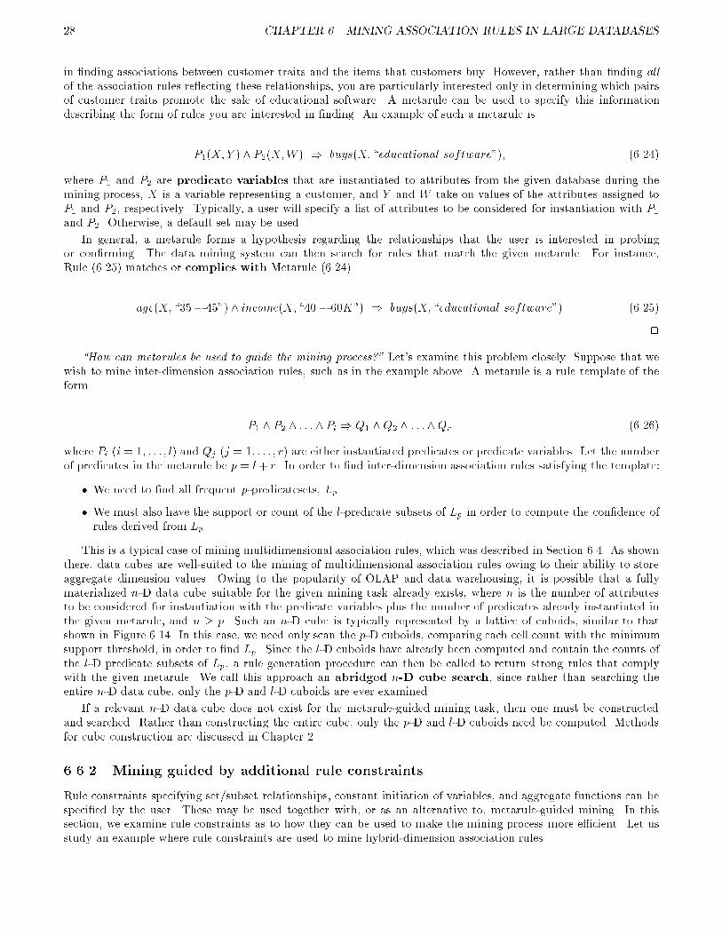
28 CHAPTER 6. MINING ASSOCIATION RULES IN LARGE DATABASES
in �nding associations between customer traits and the items that customers buy. However, rather than �nding all
of the association rules re ecting these relationships, you are particularly interested only in determining which pairsof customer traits promote the sale of educational software. A metarule can be used to specify this informationdescribing the form of rules you are interested in �nding. An example of such a metarule is
P1(X;Y ) ^ P2(X;W ) ) buys(X; \educational software"); (6.24)
where P1 and P2 are predicate variables that are instantiated to attributes from the given database during themining process, X is a variable representing a customer, and Y and W take on values of the attributes assigned toP1 and P2, respectively. Typically, a user will specify a list of attributes to be considered for instantiation with P1and P2. Otherwise, a default set may be used.
In general, a metarule forms a hypothesis regarding the relationships that the user is interested in probingor con�rming. The data mining system can then search for rules that match the given metarule. For instance,Rule (6.25) matches or complies with Metarule (6.24).
age(X; \35� 45") ^ income(X; \40 � 60K") ) buys(X; \educational software") (6.25)
2
\How can metarules be used to guide the mining process?" Let's examine this problem closely. Suppose that wewish to mine inter-dimension association rules, such as in the example above. A metarule is a rule template of theform
P1 ^ P2 ^ : : :^ Pl ) Q1 ^Q2 ^ : : :^Qr (6.26)
where Pi (i = 1; : : : ; l) and Qj (j = 1; : : : ; r) are either instantiated predicates or predicate variables. Let the numberof predicates in the metarule be p = l+ r. In order to �nd inter-dimension association rules satisfying the template:
� We need to �nd all frequent p-predicatesets, Lp.
� We must also have the support or count of the l-predicate subsets of Lp in order to compute the con�dence ofrules derived from Lp.
This is a typical case of mining multidimensional association rules, which was described in Section 6.4. As shownthere, data cubes are well-suited to the mining of multidimensional association rules owing to their ability to storeaggregate dimension values. Owing to the popularity of OLAP and data warehousing, it is possible that a fullymaterialized n-D data cube suitable for the given mining task already exists, where n is the number of attributesto be considered for instantiation with the predicate variables plus the number of predicates already instantiated inthe given metarule, and n � p. Such an n-D cube is typically represented by a lattice of cuboids, similar to thatshown in Figure 6.14. In this case, we need only scan the p-D cuboids, comparing each cell count with the minimumsupport threshold, in order to �nd Lp. Since the l-D cuboids have already been computed and contain the counts ofthe l-D predicate subsets of Lp, a rule generation procedure can then be called to return strong rules that complywith the given metarule. We call this approach an abridged n-D cube search, since rather than searching theentire n-D data cube, only the p-D and l-D cuboids are ever examined.
If a relevant n-D data cube does not exist for the metarule-guided mining task, then one must be constructedand searched. Rather than constructing the entire cube, only the p-D and l-D cuboids need be computed. Methodsfor cube construction are discussed in Chapter 2.
6.6.2 Mining guided by additional rule constraints
Rule constraints specifying set/subset relationships, constant initiation of variables, and aggregate functions can bespeci�ed by the user. These may be used together with, or as an alternative to, metarule-guided mining. In thissection, we examine rule constraints as to how they can be used to make the mining process more e�cient. Let usstudy an example where rule constraints are used to mine hybrid-dimension association rules.

6.6. CONSTRAINT-BASED ASSOCIATION MINING 29
Example 6.8 Suppose that AllElectronics has a sales multidimensional database with the following inter-relatedrelations:
� sales(customer name, item name, transaction id),
� lives(customer name, region, city),
� item(item name, category, price), and
� transaction(transaction id, day, month, year),
where lives, item, and transaction are three dimension tables, linked to the fact table sales via three keys, cus-tomer name, item name, and transaction id, respectively.
Our association mining query is to \�nd the sales of what cheap items (where the sum of the prices is less than
$100) that may promote the sales of what expensive items (where the minimum price is $500) in the same category
for Vancouver customers in 1998". This can be expressed in the DMQL data mining query language as follows,where each line of the query has been enumerated to aid in our discussion.
1) mine associations as
2) lives(C; ; \V ancouver") ^ sales+(C; ?fIg; fSg) ) sales+(C; ?fJg; fTg)3) from sales4) where S.year = 1998 and T.year = 1998 and I.category = J.category5) group by C, I.category6) having sum(I.price) < 100 and min(J.price) � 5007) with support threshold = 0.018) with con�dence threshold = 0.5
Before we discuss the rule constraints, let us have a closer look at the above query. Line 1 is a knowledge typeconstraint, where association patterns are to be discovered. Line 2 speci�ed a metarule. This is an abbreviatedform for the following metarule for hybrid-dimension association rules (multidimensional association rules where therepeated predicate here is sales):
lives(C; ; \V ancouver")^ sales(C; ?I1; S1) ^ . . .^ sales(C; ?Ik; Sk) ^ I = fI1; : : : ; Ikg ^ S = fS1; : : : ; Skg
) sales(C; ?J1; T1) ^ . . .^ sales(C; ?Jm; Tm) ^ J = fJ1; : : : ; Jmg ^ T = fT1; : : : ; Tmg
which means that one or more sales records in the form of \sales(C; ?I1; S1) ^ . . . sales(C; ?Ik; Sk)" will reside atthe rule antecedent (left-hand side), and the question mark \?" means that only item name, I1, . . . , Ik need beprinted out. \I = fI1; : : : ; Ikg" means that all the I's at the antecedent are taken from a set I, obtained from theSQL-like where-clause of line 4. Similar notational conventions are used at the consequent (right-hand side).
The metarule may allow the generation of association rules like the following.
lives(C; ; \V ancouver") ^ sales(C; \Census CD"; )^
sales(C; \MS=Office97"; ) ) sales(C; \MS=SQLServer"; ); [1:5%; 68%] (6.27)
which means that if a customer in Vancouver bought \Census CD" and \MS/O�ce97", it is likely (with a probabilityof 68%) that she will buy \MS/SQLServer", and 1.5% of all of the customers bought all three.
Data constraints are speci�ed in the \lives( ; ; \V ancouver")" portion of the metarule (i.e., all the customerswhose city is Vancouver), and in line 3, which speci�es that only the fact table, sales, need be explicitly referenced.In such a multidimensional database, variable reference is simpli�ed. For example, \S.year = 1998" is equivalent tothe SQL statement \from sales S, transaction R where S.transaction id = R.transaction id and R.year = 1998".
All three dimensions (lives, item, and transaction) are used. Level constraints are as follows: for lives, we considerjust customer name since only city = \Vancouver" is used in the selection; for item, we consider the levels item name
and category since they are used in the query; and for transaction, we are only concerned with transaction id sinceday and month are not referenced and year is used only in the selection.
Rule constraints include most portions of the where (line 4) and having (line 6) clauses, such as \S.year =
1998", \T.year = 1998", \I.category = J.category", \sum(I.price) � 100" and \min(J.price) � 500". Finally, lines

30 CHAPTER 6. MINING ASSOCIATION RULES IN LARGE DATABASES
1-var Constraint Anti-Monotone Succinct
S�v, � 2 f=;�;�g yes yes
v 2 S no yesS � V no yesS � V yes yesS = V partly yes
min(S) � v no yesmin(S) � v yes yesmin(S) = v partly yes
max(S) � v yes yes
max(S) � v no yesmax(S) = v partly yes
count(S) � v yes weakly
count(S) � v no weaklycount(S) = v partly weakly
sum(S) � v yes nosum(S) � v no nosum(S) = v partly no
avg(S)�v, � 2 f=;�;�g no no
(frequency constraint) (yes) (no)
Table 6.3: Characterization of 1-variable constraints: anti-monotonicity and succinctness.
7 and 8 specify two interestingness constraints (i.e., thresholds), namely, a minimum support of 1% and a minimumcon�dence of 50%. 2
Knowledge type and data constraints are applied before mining. The remaining constraint types could be usedafter mining, to �lter out discovered rules. This, however, maymake the mining process very ine�cient and expensive.Dimension/level constraints were discussed in Section 6.3.2, and interestingness constraints have been discussedthroughout this chapter. Let's focus now on rule constraints.
\What kind of constraints can be used during the mining process to prune the rule search space?", you ask.\More speci�cally, what kind of rule constraints can be \pushed" deep into the mining process and still ensure the
completeness of the answers to a mining query?"
Consider the rule constraint \sum(I.price) � 100" of Example 6.8. Suppose we are using an Apriori-like (level-wise) framework, which for each iteration k, explores itemsets of size k. Any itemset whose price summation is notless than 100 can be pruned from the search space, since further addition of more items to this itemset will makeit more expensive and thus will never satisfy the constraint. In other words, if an itemset does not satisfy this ruleconstraint, then none of its supersets can satisfy the constraint either. If a rule constraint obeys this property, it iscalled anti-monotone, or downward closed. Pruning by anti-monotone rule constraints can be applied at eachiteration of Apriori-style algorithms to help improve the e�ciency of the overall mining process, while guaranteeingcompleteness of the data mining query response.
Note that the Apriori property, which states that all non-empty subsets of a frequent itemset must also befrequent, is also anti-monotone. If a given itemset does not satisfy minimum support, then none of its supersets caneither. This property is used at each iteration of the Apriori algorithm to reduce the number of candidate itemsetsexamined, thereby reducing the search space for association rules.
Other examples of anti-monotone constraints include \min(J.price) � 500" and \S.year = 1998". Any itemsetwhich violates either of these constraints can be discarded since adding more items to such itemsets can never satisfythe constraints. A constraint such as \avg(I.price) � 100" is not anti-monotone. For a given set that does not satisfythis constraint, a superset created by adding some (cheap) items may result in satisfying the constraint. Hence,pushing this constraint inside the mining process will not guarantee completeness of the data mining query response.A list of 1-variable constraints, characterized on the notion of anti-monotonicity, is given in the second column ofTable 6.3.
\What other kinds of constraints can we use for pruning the search space?" Apriori-like algorithms deal with otherconstraints by �rst generating candidate sets and then testing them for constraint satisfaction, thereby following agenerate-and-test paradigm. Instead, is there a kind of constraint for which we can somehow enumerate all and only
those sets that are guaranteed to satisfy the constraint? This property of constraints is called succintness. If a rule

6.7. SUMMARY 31
constraint is succinct, then we can directly generate precisely those sets that satisfy it, even before support countingbegins. This avoids the substantial overhead of the generate-and-test paradigm. In other words, such constraints arepre-counting prunable. Let's study an example of how succinct constraints can be used in mining association rules.
Example 6.9 Based on Table 6.3, the constraint \min(J:price) � 500" is succinct. This is because we can explicitlyand precisely generate all the sets of items satisfying the constraint. Speci�cally, such a set must contain at leastone item whose price is less than $500. It is of the form: S1 [ S2, where S1 6= ; is a subset of the set of all thoseitems with prices less than $500, and S2, possibly empty, is a subset of the set of all those items with prices > $500.Because there is a precise \formula" to generate all the sets satisfying a succinct constraint, there is no need toiteratively check the rule constraint during the mining process.
What about the constraint \min(J:price) � 500", which occurs in Example 6.8? This is also succinct, since wecan generate all sets of items satisfying the constraint. In this case, we simply do not include items whose price isless than $500, since they cannot be in any set that would satisfy the given constraint. 2
Note that a constraint such as \avg(I:price) � 100" could not be pushed into the mining process, since it isneither anti-monotone nor succinct according to Table 6.3.
Although optimizations associated with succinctness (or anti-monotonicity) cannot be applied to constraints like\avg(I:price) � 100", heuristic optimization strategies are applicable and can often lead to signi�cant pruning.
6.7 Summary
� The discovery of association relationships among huge amounts of data is useful in selective marketing, decisionanalysis, and business management. A popular area of application is market basket analysis, which studiesthe buying habits of customers by searching for sets of items that are frequently purchased together (or insequence). Association rule mining consists of �rst �nding frequent itemsets (set of items, such as Aand B, satisfying a minimum support threshold, or percentage of the task-relevant tuples), from which strongassociation rules in the form of A ) B are generated. These rules also satisfy a minimum con�dence threshold
(a prespeci�ed probability of satisfying B under the condition that A is satis�ed).
� Association rules can be classi�ed into several categories based on di�erent criteria, such as:
1. Based on the types of values handled in the rule, associations can be classi�ed into Boolean vs. quan-titative.
A Boolean association shows relationships between discrete (categorical) objects. A quantitative associa-tion is a multidimensional association that involves numeric attributes which are discretized dynamically.It may involve categorical attributes as well.
2. Based on the dimensions of data involved in the rules, associations can be classi�ed into single-dimensionalvs. multidimensional.
Single-dimensional association involves a single predicate or dimension, such as buys; whereas multi-dimensional association involves multiple (distinct) predicates or dimensions. Single-dimensional as-sociation shows intra-attribute relationships (i.e., associations within one attribute or dimension);whereas multidimensional association shows inter-attribute relationships (i.e., between or among at-tributes/dimensions).
3. Based on the levels of abstractions involved in the rule, associations can be classi�ed into single-level vs.multilevel.
In a single-level association, the items or predicates mined are not considered at di�erent levels of abstrac-tion, whereas a multilevel association does consider multiple levels of abstraction.
� The Apriori algorithm is an e�cient association rule mining algorithm which explores the level-wise miningproperty: all the subsets of a frequent itemset must also be frequent. At the k-th iteration (for k > 1), it formsfrequent (k + 1)-itemset candidates based on the frequent k-itemsets, and scans the database once to �nd thecomplete set of frequent (k + 1)-itemsets, Lk+1.

32 CHAPTER 6. MINING ASSOCIATION RULES IN LARGE DATABASES
Variations involving hashing and data scan reduction can be used to make the procedure more e�cient. Othervariations include partitioning the data (mining on each partition and them combining the results), and sam-pling the data (mining on a subset of the data). These variations can reduce the number of data scans requiredto as little as two or one.
� Multilevel association rules can be mined using several strategies, based on how minimum support thresh-olds are de�ned at each level of abstraction. When using reduced minimum support at lower levels, pruningapproaches include level-cross-�ltering by single item and level-cross �ltering by k-itemset. Redundant mul-tilevel (descendent) association rules can be eliminated from presentation to the user if their support andcon�dence are close to their expected values, based on their corresponding ancestor rules.
� Techniques for miningmultidimensional association rules can be categorized according to their treatmentof quantitative attributes. First, quantitative attributes may be discretized statically, based on prede�nedconcept hierarchies. Data cubes are well-suited to this approach, since both the data cube and quantitativeattributes can make use of concept hierarchies. Second, quantitative association rules can be mined wherequantitative attributes are discretized dynamically based on binning, where \adjacent" association rules maybe combined by clustering. Third, distance-based association rules can be mined to capture the semanticsof interval data, where intervals are de�ned by clustering.
� Not all strong association rules are interesting. Correlation rules can be mined for items that are statisticallycorrelated.
� Constraint-based mining allow users to focus the search for rules by providing metarules, (i.e., pattern tem-plates) and additional mining constraints. Such mining is facilitated with the use of a declarative data miningquery language and user interface, and poses great challenges for mining query optimization. In particular, therule constraint properties of anti-monotonicity and succinctness can be used during mining to guide theprocess, leading to more e�cient and e�ective mining.
� Association rules should not be used for directly for prediction without further analysis or domain knowledge.They do not necessarily indicate causation. They are, however, a helpful starting point for further exploration,making them a popular tool for understanding data.
Exercises
1. The Apriori algorithm makes use of prior knowledge of subset support properties.
(a) Prove that all non-empty subsets of a frequent itemset must also be frequent.
(b) Prove that the support of any non-empty subset s0 of itemset s must be as great as the support of s.
(c) Given frequent itemset l and subset s of l, prove that the con�dence of the rule \s0 ) (l� s0)" cannot bemore than the con�dence of \s) (l � s)", where s0 is a subset of s.
(d) A partitioning variation of Apriori subdivides the transactions of a database D into n non-overlappingpartitions. Prove that any itemset that is frequent in D must be frequent in at least one partition of D.
2. Section 6.2.2 describes a method for generating association rules from frequent itemsets. Propose a moree�cient method. Explain why it is more e�cient than the one proposed in Section 6.2.2. (Hint: Considerincorporating the properties of Question 1b and 1c into your design).
3. A database has four transactions. Let min sup = 60% and min conf = 80%.
TID date items bought
100 10/15/99 fK, A, D, Bg
200 10/15/99 fD, A, C, E, Bg
300 10/19/99 fC, A, B, E g
400 10/22/99 fB, A, Dg
List

6.7. SUMMARY 33
(a) the frequent k-itemset for the largest k, and
(b) all of the strong association rules (with support and con�dence) matching the following metarule:
8x 2 transaction; buys(x; item1) ^ buys(x; item2) ) buys(x; item3) [s; c].
4. A database has four transactions. Let min sup = 60% and min conf = 80%.
cust ID TID items bought (in the form of brand-item category)01 100 fKing's-Crab, Sunset-Milk, Dairyland-Cheese, Best-Breadg
02 200 fBest-Cheese, Dairyland-Milk, Goldenfarm-Apple, Tasty-Pie, Wonder-Breadg01 300 fWestcoast-Apple, Dairyland-Milk, Wonder-Bread, Tasty-Pieg
03 400 fWonder-Bread, Sunset-Milk, Dairyland-Cheeseg
(a) At the granularity of item category ( e.g., itemi could be \Milk"), for the following rule template,
8X 2 transaction; buys(X; item1) ^ buys(X; item2) ) buys(X; item3)
list
i. the frequent k-itemset for the largest k, and
ii. all of the strong association rules (with their support and con�dence) containing the frequent k-itemsetfor the largest k.
(b) At the granularity of brand-item category (e.g., itemi could be \Sunset-Milk"), for the following ruletemplate,
8X 2 customer; buys(X; item1) ^ buys(X; item2) ) buys(X; item3);
list the frequent k-itemset for the largest k. Note: do not print any rules.
5. State how the partitioning method may improve the e�ciency of association mining.
6. Suppose that a large store has a transaction database that is distributed among four locations. Transactions ineach component database have the same format, namely Tj : fi1; : : : ; img, where Tj is a transaction identi�er,and ik (1 � k � m) is the identi�er of an item purchased in the transaction. Propose an e�cient algorithm tomine global association rules (without considering multilevel associations). You may present your algorithm inthe form of an outline. Your algorithm should not require shipping all of the data to one site and should notcause excessive network communication overhead.
7. Suppose that frequent itemsets are saved for a large transaction database, DB. Discuss how to e�ciently minethe (global) association rules under the same minimum support threshold, if a set of new transactions, denotedas �DB, is (incrementally) added in?
8. Suppose that a data relation describing students at Big-University has been generalized to the following gen-eralized relation R.

34 CHAPTER 6. MINING ASSOCIATION RULES IN LARGE DATABASES
major status age nationality gpa count
French M.A 30 Canada 2.8 3.2 3
cs junior 15 20 Europe 3.2 3.6 29
physics M.S 25 30 Latin America 3.2 3.6 18
engineering Ph.D 25 30 Asia 3.6 4.0 78
philosophy Ph.D 25 30 Europe 3.2 3.6 5
French senior 15 20 Canada 3.2 3.6 40
chemistry junior 20 25 USA 3.6 4.0 25
cs senior 15 20 Canada 3.2 3.6 70
philosophy M.S 30 Canada 3.6 4.0 15
French junior 15 20 USA 2.8 3.2 8
philosophy junior 25 30 Canada 2.8 3.2 9
philosophy M.S 25 30 Asia 3.2 3.6 9
French junior 15 20 Canada 3.2 3.6 52
math senior 15 20 USA 3.6 4.0 32
cs junior 15 20 Canada 3.2 3.6 76
philosophy Ph.D 25 30 Canada 3.6 4.0 14
philosophy senior 25 30 Canada 2.8 3.2 19
French Ph.D 30 Canada 2.8 3.2 1
engineering junior 20 25 Europe 3.2 3.6 71
math Ph.D 25 30 Latin America 3.2 3.6 7
chemistry junior 15 20 USA 3.6 4.0 46
engineering junior 20 25 Canada 3.2 3.6 96
French M.S 30 Latin America 3.2 3.6 4
philosophy junior 20 25 USA 2.8 3.2 8
math junior 15 20 Canada 3.6 4.0 59
Let the concept hierarchies be as follows.
status : ffreshman; sophomore; junior; seniorg 2 undergraduate.
fM:Sc:;M:A:;Ph:D:g 2 graduate.
major : fphysics; chemistry;mathg 2 science.fcs; engineeringg 2 appl: sciences.
fFrench; philosophyg 2 arts.
age : f15 20; 21 25g 2 young.f26 30; 30 g 2 old.
nationality : fAsia;Europe; U:S:A:;Latin Americag 2 foreign.
Let the minimum support threshold be 2% and the minimum con�dence threshold be 50% (at each of thelevels).
(a) Draw the concept hierarchies for status, major, age, and nationality.
(b) Find the set of strong multilevel association rules in R using uniform support for all levels.
(c) Find the set of strong multilevel association rules in R using level-cross �ltering by single items, where areduced support of 1% is used for the lowest abstraction level.
9. Propose and outline a level-shared mining approach to mining multilevel association rules in which eachitem is encoded by its level position, and an initial scan of the database collects the count for each item at each
concept level, identifying frequent and subfrequent items. Comment on the processing cost of mining multilevelassociations with this method in comparison to mining single-level associations.
10. Show that the support of an itemset H that contains both an item h and its ancestor h will be the same as thesupport for the itemset H � h. Explain how this can be used in cross-level association rule mining.
11. When mining cross-level association rules, suppose it is found that the itemset \fIBM home computer, printerg"does not satisfy minimum support. Can this information be used to prune the mining of a \descendent" itemsetsuch as \fIBM home computer, b/w printerg"? Give a general rule explaining how this information may beused for pruning the search space.

6.7. SUMMARY 35
12. Propose a method for mining hybrid-dimension association rules (multidimensional association rules with re-peating predicates).
13. Give a short example to show that items in a strong association rule may actually be negatively correlated.
14. The following contingency table summarizes supermarket transaction data, where hot dogs refer to the trans-actions containing hot dogs, hotdogs refer to the transactions which do not contain hot dogs, hamburgers referto the transactions containing hamburgers, and hamburgers refer to the transactions which do not containhamburgers.
hot dogs hotdogs �row
hamburgers 2,000 500 2,500
hamburgers 1,000 1,500 2,500
�col 3,000 2,000 5,000
(a) Suppose that the association rule \hot dogs) hamburgers" is mined. Given a minimumsupport thresholdof 25% and a minimum con�dence threshold of 50%, is this association rule strong?
(b) Based on the given data, is the purchase of hot dogs independent of the purchase of hamburgers? If not,what kind of correlation relationship exists between the two?
15. Sequential patterns can be mined in methods similar to the mining of association rules. Design an e�cientalgorithm to minemultilevel sequential patterns from a transaction database. An example of such a patternis the following: \a customer who buys a PC will buy Microsoft software within three months", on which onemay drill-down to �nd a more re�ned version of the pattern, such as \a customer who buys a Pentium Pro will
buy Microsoft O�ce'97 within three months".
16. Prove the characterization of the following 1-variable rule constraints with respect to anti-monotonicity andsuccinctness.
1-var Constraint Anti-Monotone Succinct
a) v 2 S no yesb) min(S) � v no yesc) min(S) � v yes yesd) max(S) � v yes yes
17. The price of each item in a store is nonnegative. The store manager is only interested in rules of the form: \onefree item may trigger $200 total purchases in the same transaction". State how to mine such rules e�ciently.
18. The price of each item in a store is nonnegative. For each of the following cases, identify the kinds of constraint
they represent and brie y discuss how to mine such association rules e�ciently.
(a) containing at least one Nintendo game
(b) containing items whose sum of the prices is less than $150
(c) containing one free item and other items whose sum of the prices is at least $200 in total.
Bibliographic Notes
Association rule mining was �rst proposed by Agrawal, Imielinski, and Swami [1]. The Apriori algorithm discussedin Section 6.2.1 was presented by Agrawal and Srikant [4], and a similar level-wise association mining algorithm wasdeveloped by Klemettinen et al. [20]. A method for generating association rules is described in Agrawal and Srikant[3]. References for the variations of Apriori described in Section 6.2.3 include the following. The use of hash tablesto improve association mining e�ciency was studied by Park, Chen, and Yu [29]. Transaction reduction techniquesare described in Agrawal and Srikant [4], Han and Fu [16], and Park, Chen and Yu [29]. The partitioning techniquewas proposed by Savasere, Omiecinski and Navathe [33]. The sampling approach is discussed in Toivonen [41]. Adynamic itemset counting approach is given in Brin et al. [9]. Calendric market basket analysis is discussed in

36 CHAPTER 6. MINING ASSOCIATION RULES IN LARGE DATABASES
Ramaswamy, Mahajan, and Silberschatz [32]. Mining of sequential patterns is described in Agrawal and Srikant [5],and Mannila, Toivonen, and Verkamo [24].
Multilevel association mining was studied in Han and Fu [16], and Srikant and Agrawal [38]. In Srikant andAgrawal [38], such mining is studied in the context of generalized association rules, and an R-interest measure isproposed for removing redundant rules.
Mining multidimensional association rules using static discretization of quantitative attributes and data cubeswas studied by Kamber, Han, and Chiang [19]. Zhao, Deshpande, and Naughton [43] found that even when a cube isconstructed on the y, mining from data cubes can be faster than mining directly from a relational table. The ARCSsystem described in Section 6.4.3 for mining quantitative association rules based on rule clustering was proposed byLent, Swami, and Widom [22]. Techniques for mining quantitative rules based on x-monotone and rectilinear regionswere presented by Fukuda et al. [15], and Yoda et al. [42]. A non-grid-based technique for mining quantitativeassociation rules, which uses a measure of partial completeness, was proposed by Srikant and Agrawal [39]. Theapproach described in Section 6.4.4 for mining (distance-based) association rules over interval data was proposed byMiller and Yang [26].
The statistical independence of rules in data mining was studied by Piatetski-Shapiro [31]. The interestingnessproblem of strong association rules is discussed by Chen, Han, and Yu [10], and Brin, Motwani, and Silverstein [8].An e�cient method for generalizing associations to correlations is given in Brin, Motwani, and Silverstein [8], andbrie y summarized in Section 6.5.2.
The use of metarules as syntactic or semantic �lters de�ning the form of interesting single-dimensional associationrules was proposed in Klemettinen et al. [20]. Metarule-guided mining, where the metarule consequent speci�es anaction (such as Bayesian clustering or plotting) to be applied to the data satisfying the metarule antecedent, wasproposed in Shen et al. [35]. A relation-based approach to metarule-guided mining of association rules is studied inFu and Han [14]. A data cube-based approach is studied in Kamber et al. [19]. The constraint-based associationrule mining of Section 6.6.2 was studied in Ng et al. [27] and Lakshmanan et al. [21]. Other ideas involving the useof templates or predicate constraints in mining have been discussed in [6, 13, 18, 23, 36, 40].
An SQL-like operator for mining single-dimensional association rules was proposed by Meo, Psaila, and Ceri [25],and further extended in Baralis and Psaila [7]. The data mining query language, DMQL, was proposed in Han etal. [17].
An e�cient incremental updating of mined association rules was proposed by Cheung et al. [12]. Parallel anddistributed association data mining under the Apriori framework was studied by Park, Chen, and Yu [30], Agrawaland Shafer [2], and Cheung et al. [11]. Additional work in the mining of association rules includes mining sequentialassociation patterns by Agrawal and Srikant [5], mining negative association rules by Savasere, Omiecinski andNavathe [34], and mining cyclic association rules by Ozden, Ramaswamy, and Silberschatz [28].

Bibliography
[1] R. Agrawal, T. Imielinski, and A. Swami. Mining association rules between sets of items in large databases. InProc. 1993 ACM-SIGMOD Int. Conf. Management of Data, pages 207{216, Washington, D.C., May 1993.
[2] R. Agrawal and J. C. Shafer. Parallel mining of association rules: Design, implementation, and experience.IEEE Trans. Knowledge and Data Engineering, 8:962{969, 1996.
[3] R. Agrawal and R. Srikant. Fast algorithm for mining association rules in large databases. In Research Report
RJ 9839, IBM Almaden Research Center, San Jose, CA, June 1994.
[4] R. Agrawal and R. Srikant. Fast algorithms for mining association rules. In Proc. 1994 Int. Conf. Very Large
Data Bases, pages 487{499, Santiago, Chile, September 1994.
[5] R. Agrawal and R. Srikant. Mining sequential patterns. In Proc. 1995 Int. Conf. Data Engineering, pages 3{14,Taipei, Taiwan, March 1995.
[6] T. Anand and G. Kahn. Opportunity explorer: Navigating large databases using knowledge discovery templates.In Proc. AAAI-93 Workshop Knowledge Discovery in Databases, pages 45{51, Washington DC, July 1993.
[7] E. Baralis and G. Psaila. Designing templates for mining association rules. Journal of Intelligent InformationSystems, 9:7{32, 1997.
[8] S. Brin, R. Motwani, and C. Silverstein. Beyond market basket: Generalizing association rules to correlations.In Proc. 1997 ACM-SIGMOD Int. Conf. Management of Data, pages 265{276, Tucson, Arizona, May 1997.
[9] S. Brin, R. Motwani, J. D. Ullman, and S. Tsur. Dynamic itemset counting and implication rules for marketbasket analysis. In Proc. 1997 ACM-SIGMOD Int. Conf. Management of Data, pages 255{264, Tucson, Arizona,May 1997.
[10] M. S. Chen, J. Han, and P. S. Yu. Data mining: An overview from a database perspective. IEEE Trans.
Knowledge and Data Engineering, 8:866{883, 1996.
[11] D.W. Cheung, J. Han, V. Ng, A. Fu, and Y. Fu. A fast distributed algorithm for mining association rules. InProc. 1996 Int. Conf. Parallel and Distributed Information Systems, pages 31{44, Miami Beach, Florida, Dec.1996.
[12] D.W. Cheung, J. Han, V. Ng, and C.Y. Wong. Maintenance of discovered association rules in large databases:An incremental updating technique. In Proc. 1996 Int. Conf. Data Engineering, pages 106{114, New Orleans,Louisiana, Feb. 1996.
[13] V. Dhar and A. Tuzhilin. Abstract-driven pattern discovery in databases. IEEE Trans. Knowledge and Data
Engineering, 5:926{938, 1993.
[14] Y. Fu and J. Han. Meta-rule-guided mining of association rules in relational databases. In Proc. 1st Int.
Workshop Integration of Knowledge Discovery with Deductive and Object-Oriented Databases (KDOOD'95),pages 39{46, Singapore, Dec. 1995.
[15] T. Fukuda, Y. Morimoto, S. Morishita, and T. Tokuyama. Data mining using two-dimensional optimizedassociation rules: Scheme, algorithms, and visualization. In Proc. 1996 ACM-SIGMOD Int. Conf. Management
of Data, pages 13{23, Montreal, Canada, June 1996.
37

38 BIBLIOGRAPHY
[16] J. Han and Y. Fu. Discovery of multiple-level association rules from large databases. In Proc. 1995 Int. Conf.
Very Large Data Bases, pages 420{431, Zurich, Switzerland, Sept. 1995.
[17] J. Han, Y. Fu, W. Wang, K. Koperski, and O. R. Za��ane. DMQL: A data mining query language for relationaldatabases. In Proc. 1996 SIGMOD'96 Workshop Research Issues on Data Mining and Knowledge Discovery
(DMKD'96), pages 27{34, Montreal, Canada, June 1996.
[18] P. Hoschka and W. Kl�osgen. A support system for interpreting statistical data. In G. Piatetsky-Shapiro andW. J. Frawley, editors, Knowledge Discovery in Databases, pages 325{346. AAAI/MIT Press, 1991.
[19] M. Kamber, J. Han, and J. Y. Chiang. Metarule-guided mining of multi-dimensional association rules usingdata cubes. In Proc. 3rd Int. Conf. Knowledge Discovery and Data Mining (KDD'97), pages 207{210, NewportBeach, California, August 1997.
[20] M. Klemettinen, H. Mannila, P. Ronkainen, H. Toivonen, and A.I. Verkamo. Finding interesting rules from largesets of discovered association rules. In Proc. 3rd Int. Conf. Information and Knowledge Management, pages401{408, Gaithersburg, Maryland, Nov. 1994.
[21] L. V. S. Lakshmanan, R. Ng, J. Han, and A. Pang. Optimization of constrained frequent set queries with 2-variable constraints. In Proc. 1999 ACM-SIGMOD Int. Conf. Management of Data, pages 157{168, Philadelphia,PA, June 1999.
[22] B. Lent, A. Swami, and J. Widom. Clustering association rules. In Proc. 1997 Int. Conf. Data Engineering
(ICDE'97), pages 220{231, Birmingham, England, April 1997.
[23] B. Liu, W. Hsu, and S. Chen. Using general impressions to analyze discovered classi�cation rules. In Proc. 3rd
Int.. Conf. on Knowledge Discovery and Data Mining (KDD'97), pages 31{36, Newport Beach, CA, August1997.
[24] H. Mannila, H Toivonen, and A. I. Verkamo. Discovering frequent episodes in sequences. In Proc. 1st Int. Conf.
Knowledge Discovery and Data Mining, pages 210{215, Montreal, Canada, Aug. 1995.
[25] R. Meo, G. Psaila, and S. Ceri. A new SQL-like operator for mining association rules. In Proc. 1996 Int. Conf.
Very Large Data Bases, pages 122{133, Bombay, India, Sept. 1996.
[26] R.J. Miller and Y. Yang. Association rules over interval data. In Proc. 1997 ACM-SIGMOD Int. Conf. Man-
agement of Data, pages 452{461, Tucson, Arizona, May 1997.
[27] R. Ng, L. V. S. Lakshmanan, J. Han, and A. Pang. Exploratory mining and pruning optimizations of con-strained associations rules. In Proc. 1998 ACM-SIGMOD Int. Conf. Management of Data, pages 13{24, Seattle,Washington, June 1998.
[28] B. �Ozden, S. Ramaswamy, and A. Silberschatz. Cyclic association rules. In Proc. 1998 Int. Conf. Data Engi-
neering (ICDE'98), pages 412{421, Orlando, FL, Feb. 1998.
[29] J.S. Park, M.S. Chen, and P.S. Yu. An e�ective hash-based algorithm for mining association rules. In Proc.
1995 ACM-SIGMOD Int. Conf. Management of Data, pages 175{186, San Jose, CA, May 1995.
[30] J.S. Park, M.S. Chen, and P.S. Yu. E�cient parallel mining for association rules. In Proc. 4th Int. Conf.
Information and Knowledge Management, pages 31{36, Baltimore, Maryland, Nov. 1995.
[31] G. Piatetsky-Shapiro. Discovery, analysis, and presentation of strong rules. In G. Piatetsky-Shapiro and W. J.Frawley, editors, Knowledge Discovery in Databases, pages 229{238. AAAI/MIT Press, 1991.
[32] S. Ramaswamy, S. Mahajan, and A. Silberschatz. On the discovery of interesting patterns in association rules.In Proc. 1998 Int. Conf. Very Large Data Bases, pages 368{379, New York, NY, August 1998.
[33] A. Savasere, E. Omiecinski, and S. Navathe. An e�cient algorithm for mining association rules in large databases.In Proc. 1995 Int. Conf. Very Large Data Bases, pages 432{443, Zurich, Switzerland, Sept. 1995.

BIBLIOGRAPHY 39
[34] A. Savasere, E. Omiecinski, and S. Navathe. Mining for strong negative associations in a large database ofcustomer transactions. In Proc. 1998 Int. Conf. Data Engineering (ICDE'98), pages 494{502, Orlando, FL,Feb. 1998.
[35] W. Shen, K. Ong, B. Mitbander, and C. Zaniolo. Metaqueries for data mining. In U.M. Fayyad, G. Piatetsky-Shapiro, P. Smyth, and R. Uthurusamy, editors, Advances in Knowledge Discovery and Data Mining, pages375{398. AAAI/MIT Press, 1996.
[36] A. Silberschatz and A. Tuzhilin. What makes patterns interesting in knowledge discovery systems. IEEE
Trans. on Knowledge and Data Engineering, 8:970{974, Dec. 1996.
[37] E. Simoudis, J. Han, and U. Fayyad (eds.). Proc. 2nd Int. Conf. Knowledge Discovery and Data Mining
(KDD'96). AAAI Press, August 1996.
[38] R. Srikant and R. Agrawal. Mining generalized association rules. In Proc. 1995 Int. Conf. Very Large Data
Bases, pages 407{419, Zurich, Switzerland, Sept. 1995.
[39] R. Srikant and R. Agrawal. Mining quantitative association rules in large relational tables. In Proc. 1996
ACM-SIGMOD Int. Conf. Management of Data, pages 1{12, Montreal, Canada, June 1996.
[40] R. Srikant, Q. Vu, and R. Agrawal. Mining association rules with item constraints. In Proc. 3rd Int. Conf.
Knowledge Discovery and Data Mining (KDD'97), pages 67{73, Newport Beach, California, August 1997.
[41] H. Toivonen. Sampling large databases for association rules. In Proc. 1996 Int. Conf. Very Large Data Bases,pages 134{145, Bombay, India, Sept. 1996.
[42] K. Yoda, T. Fukuda, Y. Morimoto, S. Morishita, and T. Tokuyama. Computing optimized rectilinear regionsfor association rules. In Proc. 3rd Int. Conf. Knowledge Discovery and Data Mining (KDD'97), pages 96{103,Newport Beach, California, August 1997.
[43] Y. Zhao, P. M. Deshpande, and J. F. Naughton. An array-based algorithm for simultaneous multidimensionalaggregates. In Proc. 1997 ACM-SIGMOD Int. Conf. Management of Data, pages 159{170, Tucson, Arizona,May 1997.