computing primer for applied linear regression, third - people
TRANSCRIPT

Computing Primerfor
Applied LinearRegression, Third Edition
Using R and S-Plus
Sanford WeisbergUniversity of Minnesota
School of StatisticsJune 7, 2005
c©2005, Sanford Weisberg
Home Website: www.stat.umn.edu/alr


Contents
Introduction 10.1 Organization of this primer 40.2 Data files 5
0.2.1 Documentation 50.2.2 R data files and a package 60.2.3 S-Plus data files and library 60.2.4 Getting the data in text files 70.2.5 An exceptional file 7
0.3 Scripts 70.4 The very basics 8
0.4.1 Reading a data file 80.4.2 Saving text output and graphs 90.4.3 Normal, F , t and χ2 tables 10
0.5 Abbreviations to remember 100.6 Packages/Libraries for R and S-Plus 100.7 Copyright and Printing this Primer 11
1 Scatterplots and Regression 131.1 Scatterplots 131.2 Mean functions 16
v

vi CONTENTS
1.3 Variance functions 161.4 Summary graph 161.5 Tools for looking at scatterplots 161.6 Scatterplot matrices 16
2 Simple Linear Regression 192.1 Ordinary least squares estimation 192.2 Least squares criterion 192.3 Estimating σ2 202.4 Properties of least squares estimates 202.5 Estimated variances 202.6 Comparing models: The analysis of variance 212.7 The coefficient of determination, R2 222.8 Confidence intervals and tests 232.9 The Residuals 26
3 Multiple Regression 273.1 Adding a term to a simple linear regression model 273.2 The Multiple Linear Regression Model 273.3 Terms and Predictors 273.4 Ordinary least squares 283.5 The analysis of variance 303.6 Predictions and fitted values 31
4 Drawing Conclusions 334.1 Understanding parameter estimates 33
4.1.1 Rate of change 344.1.2 Sign of estimates 344.1.3 Interpretation depends on other terms in the mean function 344.1.4 Rank deficient and over-parameterized models 34
4.2 Experimentation versus observation 344.3 Sampling from a normal population 344.4 More on R2 344.5 Missing data 344.6 Computationally intensive methods 36
5 Weights, Lack of Fit, and More 415.1 Weighted Least Squares 41

CONTENTS vii
5.1.1 Applications of weighted least squares 425.1.2 Additional comments 42
5.2 Testing for lack of fit, variance known 425.3 Testing for lack of fit, variance unknown 435.4 General F testing 445.5 Joint confidence regions 45
6 Polynomials and Factors 476.1 Polynomial regression 47
6.1.1 Polynomials with several predictors 486.1.2 Using the delta method to estimate a minimum or a maximum 496.1.3 Fractional polynomials 51
6.2 Factors 516.2.1 No other predictors 536.2.2 Adding a predictor: Comparing regression lines 53
6.3 Many factors 546.4 Partial one-dimensional mean functions 546.5 Random coefficient models 56
7 Transformations 597.1 Transformations and scatterplots 59
7.1.1 Power transformations 597.1.2 Transforming only the predictor variable 597.1.3 Transforming the response only 637.1.4 The Box and Cox method 64
7.2 Transformations and scatterplot matrices 657.2.1 The 1D estimation result and linearly related predictors 667.2.2 Automatic choice of transformation of the predictors 66
7.3 Transforming the response 687.4 Transformations of non-positive variables 68
8 Regression Diagnostics: Residuals 698.1 The residuals 69
8.1.1 Difference between e and e 698.1.2 The hat matrix 698.1.3 Residuals and the hat matrix with weights 708.1.4 The residuals when the model is correct 708.1.5 The residuals when the model is not correct 70

viii CONTENTS
8.1.6 Fuel consumption data 708.2 Testing for curvature 718.3 Nonconstant variance 72
8.3.1 Variance Stabilizing Transformations 728.3.2 A diagnostic for nonconstant variance 728.3.3 Additional comments 73
8.4 Graphs for model assessment 738.4.1 Checking mean functions 738.4.2 Checking variance functions 74
9 Outliers and Influence 759.1 Outliers 75
9.1.1 An outlier test 759.1.2 Weighted least squares 769.1.3 Significance levels for the outlier test 769.1.4 Additional comments 76
9.2 Influence of cases 769.2.1 Cook’s distance 779.2.2 Magnitude of Di 779.2.3 Computing Di 779.2.4 Other measures of influence 77
9.3 Normality assumption 77
10 Variable Selection 7910.1 The Active Terms 79
10.1.1 Collinearity 8010.1.2 Collinearity and variances 81
10.2 Variable selection 8110.2.1 Information criteria 8110.2.2 Computationally intensive criteria 8110.2.3 Using subject-matter knowledge 81
10.3 Computational methods 8110.3.1 Subset selection overstates significance 87
10.4 Windmills 8710.4.1 Six mean functions 8710.4.2 A computationally intensive approach 87
11 Nonlinear Regression 89

CONTENTS ix
11.1 Estimation for nonlinear mean functions 8911.2 Inference assuming large samples 8911.3 Bootstrap inference 9311.4 References 94
12 Logistic Regression 9512.1 Binomial Regression 95
12.1.1 Mean Functions for Binomial Regression 9512.2 Fitting Logistic Regression 95
12.2.1 One-predictor example 9612.2.2 Many Terms 9712.2.3 Deviance 9812.2.4 Goodness of Fit Tests 99
12.3 Binomial Random Variables 9912.3.1 Maximum likelihood estimation 9912.3.2 The Log-likelihood for Logistic Regression 99
12.4 Generalized linear models 99
Appendix A 101A.1 Web site 101A.2 Means and variances of random variables 101
A.2.1 E notation 101A.2.2 Var notation 101A.2.3 Cov notation 101A.2.4 Conditional moments 101
A.3 Least squares for simple regression 101A.4 Means and variances of least squares estimates 101A.5 Estimating E(Y |X) using a smoother 101A.6 A brief introduction to matrices and vectors 103
A.6.1 Addition and subtraction 103A.6.2 Multiplication by a scalar 103A.6.3 Matrix multiplication 103A.6.4 Transpose of a matrix 103A.6.5 Inverse of a matrix 103A.6.6 Orthogonality 103A.6.7 Linear dependence and rank of a matrix 103
A.7 Random vectors 103A.8 Least squares using matrices 103

x CONTENTS
A.8.1 Properties of estimates 103A.8.2 The residual sum of squares 103A.8.3 Estimate of variance 103
A.9 The QR factorization 103A.10 Maximum likelihood estimates 105A.11 The Box-Cox method for transformations 105
A.11.1 Univariate case 105A.11.2 Multivariate case 105
A.12 Case deletion in linear regression 105
References 107
Index 109
0Introduction
This computer primer supplements the book Applied Linear Regression (alr),third edition, by Sanford Weisberg, published by John Wiley & Sons in 2005.It shows you how to do the analyses discussed in alr using one of severalgeneral-purpose programs that are widely available throughout the world. Allthe programs have capabilities well beyond the uses described here. Differentprograms are likely to suit different users. We expect to update the primerperiodically, so check www.stat.umn.edu/alr to see if you have the most recentversion. The versions are indicated by the date shown on the first page of theprimer.
Our purpose is largely limited to using the packages with alr, and we willnot attempt to provide a complete introduction to the packages. If you arenew to the package you are using you will probably need additional referencematerial.
There are a number of methods discussed in alr that are not (as yet)a standard part of statistical analysis, and some methods are not possiblewithout writing your own programs to supplement the package you choose.The exceptions to this rule are R and S-Plus. For these two packages we havewritten functions you can easily download and use for nearly everything in thebook.
Here are the programs for which primers are available.
R is a command line statistical package, which means that the user typesa statement requesting a computation or a graph, and it is executedimmediately. You will be able to use a package of functions for R that
1

2 INTRODUCTION
will let you use all the methods discussed in alr; we used R when writingthe book.
R also has a programming language that allows automating repetitivetasks. R is a favorite program among academic statisticians becauseit is free, works on Windows, Linux/Unix and Macintosh, and can beused in a great variety of problems. There is also a large literaturedeveloping on using R for statistical problems. The main website forR is www.r-project.org. From this website you can get to the page fordownloading R by clicking on the link for CRAN, or, in the US, going tocran.us.r-project.org.
Documentation is available for R on-line, from the website, and in severalbooks. We can strongly recommend two books. The book by Fox (2002)provides a fairly gentle introduction to R with emphasis on regression.We will from time to time make use of some of the functions discussedin Fox’s that are not in the base R program. A more comprehensiveintroduction to R is Venables and Ripley (2002), and we will use thenotation vr[3.1], for example, to refer to Section 3.1 of that book.Venables and Ripley has more computerese than does Fox’s book, butits coverage is greater and you will be able to use this book for morethan linear regression. Other books on R include Maindonald and Braun(2002), Venables and Smith (2002), and Dalgaard (2002). We used R
Version 2.0.0 on Windows and Linux. A new version of R is releasedtwice a year, so the version you use will probably be newer. If you havea fast internet connection, downloading and upgrading R is easy, andyou should do it regularly.
S-Plus is very similar to R, and most commands that work in R also work inS-Plus. Both are variants of a statistical language called “S” that waswritten at Bell Laboratories before the breakup of AT&T. Unlike R, S-
Plus is a commercial product, which means that it is not free, althoughthere is a free student version available at elms03.e-academy.com/splus.The website of the publisher is www.insightful.com/products/splus. Alibrary of functions very similar to those for R are also available thatwill make S-Plus useful for all the methods discussed in alr.
Unlike R, S-Plus has a well-developed graphical user interface or GUI.Many new users of S-Plus are likely to learn to use this program throughthe GUI, not through the command-line interface. In this primer, how-ever, we make no use of the GUI.
If you are using S-Plus on a Windows machine, you probably have themanuals that came with the program. If you are using Linux/Unix, youmay not have the manuals. In either case the manuals are availableonline; for Windows see the Hel→Online Manuals, and for Linux/Unixuse
cd ‘Splus SHOME‘/doc

3
and see the pdf documents there. Chambers and Hastie (1993) providesthe basics of fitting models with S languages like S-Plus and R. For amore general reference, we again recommend Fox (2002) and Venablesand Ripley (2002), as we did for R. We used S-Plus Version 6.0 Release1 for Linux, and S-Plus 2000 for Windows. Newer versions of both areavailable.
SAS is the largest and most widely distributed statistical package in bothindustry and education. SAS also has a GUI. While it is possible to dosome data analysis using the SAS GUI, the strength of this program is inthe ability to write SAS programs, in the editor window, and then submitthem for execution, with output returned in an output window. We willtherefore view SAS as a batch system, and concentrate mostly on writingSAS commands to be executed. The website for SAS is www.sas.com.
SAS is very widely documented, including hundreds of books availablethrough amazon.com or from the SAS Institute, and extensive on-linedocumentation. Muller and Fetterman (2003) is dedicated particularlyto regression. We used Version 9.1 for Windows. We find the on-linedocumentation that accompanies the program to be invaluable, althoughlearning to read and understand SAS documentation isn’t easy.
Although SAS is a programming language, adding new functionality canbe very awkward and require long, confusing programs. These programscould, however, be turned into SAS macros that could be reused over andover, so in principle SAS could be made as useful as R or S-Plus. We havenot done this, but would be delighted if readers would take on the chal-lenge of writing macros for methods that are awkward with SAS. Anyonewho takes this challenge can send us the results ([email protected])for inclusion in later revisions of the primer.
We have, however, prepared script files that give the programs that willproduce all the output discussed in this primer; you can get the scriptsfrom www.stat.umn.edu/alr.
JMP is another product of SAS Institute, and was designed around a cleverand useful GUI. A student version of JMP is available. The website iswww.jmp.com. We used JMP Version 5.1 on Windows.
Documentation for the student version of JMP, called JMP-In, comeswith the book written by Sall, Creighton and Lehman (2005), and we willwrite jmp-start[3] for Chapter 3 of that book, or jmp-start[P360] forpage 360. The full version of JMP includes very extensive manuals; themanuals are available on CD only with JMP-In. Fruend, Littell andCreighton (2003) discusses JMP specifically for regression.
JMP has a scripting language that could be used to add functionalityto the program. We have little experience using it, and would be happyto hear from readers on their experience using the scripting language to

4 INTRODUCTION
extend JMP to use some of the methods discussed in alr that are notpossible in JMP without scripting.
SPSS evolved from a batch program to have a very extensive graphical userinterface. In the primer we use only the GUI for SPSS, which limitsthe methods are are available. Like SAS, SPSS has many sophisticatedtools for data base management. A student version is available. Thewebsite for SPSS is www.spss.com. SPSS offers hundreds of pages ofdocumentation, including SPSS (2003), with Chapter 26 dedicated toregression models. In mid-2004, amazon.com listed more than two thou-sand books for which “SPSS” was a keyword. We used SPSS Version12.0 for Windows.
This is hardly an exhaustive list of programs that could be used for re-gression analysis. If your favorite package is missing, please take this as achallenge: try to figure out how to do what is suggested in the text, and writeyour own primer! Send us a PDF file ([email protected]) and we will addit to our website, or link to yours.
One program missing from the list of programs for regression analysis isMicrosoft’s spreadsheet program Excel. While a few of the methods describedin the book can be computed or graphed in Excel, most would require greatendurance and patience on the part of the user. There are many add-onstatistics programs for Excel, and one of these may be useful for comprehensiveregression analysis; we don’t know. If something works for you, please let usknow!
A final package for regression that we should mention is called Arc. LikeR, Arc is free software. It is available from www.stat.umn.edu/arc. Like JMP
and SPSS it is based around a graphical user interface, so most computationsare done via point-and-click. Arc also includes access to a complete computerlanguage, although the language, lisp, is considerably harder to learn than theS or SAS languages. Arc includes all the methods described in the book. Theuse of Arc is described in Cook and Weisberg (1999), so we will not discuss itfurther here; see also Weisberg (2005).
0.1 ORGANIZATION OF THIS PRIMER
The primer often refers to specific problems or sections in alr using notationlike alr[3.2] or alr[A.5], for a reference to Section 3.2 or Appendix A.5,alr[P3.1] for Problem 3.1, alr[F1.1] for Figure 1.1, alr[E2.6] for an equa-tion and alr[T2.1] for a table. Reference to, for example, “Figure 7.1,” wouldrefer to a figure in this primer, not to alr. Chapters, sections, and homeworkproblems are numbered in this primer as they are in alr. Consequently, thesection headings in primer refers to the material in alr, and not necessarilythe material in the primer. Many of the sections in this primer don’t have any

DATA FILES 5
material because that section doesn’t introduce any new issues with regard tocomputing. The index should help you navigate through the primer.
There are four versions of this primer, one for R and S-Plus, and one foreach of the other packages. All versions are available for free as PDF files atwww.stat.umn.edu/alr.
Anything you need to type into the program will always be in this font.Output from a program depends on the program, but should be clear fromcontext. We will write File to suggest selecting the menu called “File,” andTransform→Recode to suggest selecting an item called “Recode” from a menucalled “Transform.” You will sometimes need to push a button in a dialog,and we will write “push ok” to mean “click on the button marked ‘OK’.” Fornon-English versions of some of the programs, the menus may have differentnames, and we apologize in advance for any confusion this causes.
R and S-Plus Most of the graphs and computer output in alr were producedwith R. The computer code we give in this primer may not reproduce thegraphs exactly, since we have tweaked some of the graphs to make them lookprettier for publication, and the tweaking arguments work a little differentlyin R and S-Plus. If you want to see the tweaks we used in R, look at thescripts, Section 0.3.
0.2 DATA FILES
0.2.1 Documentation
Documentation for nearly all of the data files is contained in alr; lookin the index for the first reference to a data file. Separate documenta-tion can be found in the file alr3data.pdf in PDF format at the web sitewww.stat.umn.edu/alr.
The data are available in a package for R, in a library for S-Plus and for SAS,and as a directory of files in special format for JMP and SPSS. In addition,the files are available as plain text files that can be used with these, or anyother, program. Table 0.1 shows a copy of one of the smallest data files calledhtwt.txt, and described in alr[P3.1]. This file has two variables, named Htand Wt, and ten cases, or rows in the data file. The largest file is wm5.txt with62,040 cases and 14 variables. This latter file is so large that it is handleddifferently from the others; see Section 0.2.5.
A few of the data files have missing values, and these are generally indicatedin the file by a question mark “?” in the place of the missing value. Differentprograms handle missing values a little differently; we will discuss this furtherwhen we get to the first data set with a missing value in Section 4.5.

6 INTRODUCTION
Table 0.1 The data file htwt.txt.
Ht Wt
169.6 71.2
166.8 58.2
157.1 56
181.1 64.5
158.4 53
165.6 52.4
166.7 56.8
156.5 49.2
168.1 55.6
165.3 77.8
0.2.2 R data files and a package
All the data files and a few additional functions that automate methods dis-cussed in alr are collected into an R package named alr3. We recommendthat you install the package on your computer. The instructions are on theweb at www.stat.umn.edu/alr.
Once you have installed the package, two commands are required to accessa data file. First, the command
> library(alr3)
(or library(alr3,lib.loc="mylib/") if you installed your own Linux/Unix li-brary) to load the package opens the package for your use. To read a particularfile, say forbes.txt, or example, type
> data(forbes)
without the “.txt” suffix that is shown in alr. This will create a data framewith the name forbes. If you then type simply forbes, the data will be listed.You can add a new variable to the data set by typing, for example
> forbes$logTemp <- log(forbes$Temp,2)
to add the base-two logarithm of Temperature to the data frame.You can view the documentation for the data sets on-line. The most elegant
method is to enter the command help.start() into R. This will start your webbrowser, if it is not already running. Click on “Packages,” and then on “alr3.”You will then get an alphabetical listing of all the data files, and you can selectthe one you want to see.
0.2.3 S-Plus data files and library
The S-Plus data files are also available as a library; see www.stat.umn.edu/alr
for instructions on downloading and installing1.
1A library in S-Plus is called a package in R.

SCRIPTS 7
In S-Plus, you don’t need the data command to access a data set in alibrary; indeed, the data command doesn’t exist in S-Plus. To use the Forbesdata set, for example, you can use the following commands
> library(alr3)
> f <- forbes
> f$logTemp <- logb(f$Temp,2)
> f
This will load the library, and make f be a local copy of the data set forbes.In S-Plus, you need to make a local copy of the data set if you want to changeit, as we have done here by adding a new variable. In S-Plus, the commandlog computes natural logs; we need to use logb to compute logs to some otherbase. The final command prints f in the text window.
0.2.4 Getting the data in text files
You can download the data as a directory of plain text files, or as individualfiles; see www.stat.umn.edu/alr/data. Missing values on these files are indi-cated with a ?. If your program does not use this missing value character, youmay need to substitute a different character using an editor.
0.2.5 An exceptional file
The file wm5.txt is not included in any of the compressed files, or inthe libraries. This one file is nearly five megabytes long, requiring as muchspace as all the other files combined. If you need this file, for alr[P10.12],you can download it separately from www.stat.umn.edu/alr/data.
0.3 SCRIPTS
For R, S-Plus, and SAS, we have prepared script files that can be used whilereading this primer. For R and S-Plus, the scripts will reproduce nearly everycomputation shown in alr; indeed, these scripts were used to do the calcu-lations in the first place. For SAS, the scripts correspond to the discussiongiven in this primer, but will not reproduce everything in alr. The scriptscan be downloaded from www.stat.umn.edu/alr for R, S-Plus or SAS.
Although both JMP and SPSS have scripting or programming languages, wehave not prepared scripts for these programs. Some of the methods discussedin alr are not possible in these programs without the use of scripts, and sowe encourage readers to write scripts in these languages that implement theseideas. Topics that require scripts include bootstrapping and computer inten-sive methods, alr[4.6]; partial one-dimensional models, alr[6.4], inverse re-sponse plots, alr[7.1, 7.3], multivariate Box-Cox transformations, alr[7.2],

8 INTRODUCTION
Yeo-Johnson transformations, alr[7.4], and heteroscedasticity tests, alr[8.3.2].There are several other places where usability could be improved with a script.
If you write scripts you would like to share with others, let me know([email protected]) and I’ll make a link to them or add them to the web-site.
0.4 THE VERY BASICS
Before you can begin doing any useful computing, you need to be able to readdata into the program, and after you are done you need to be able to saveand print output and graphs. All the programs are a little different in howthey handle input and output, and we give some of the details here.
0.4.1 Reading a data file
Reading data into a program is surprisingly difficult. We have tried to easethis burden for you, at least when using the data files supplied with alr, byproviding the data in a special format for each of the programs. There willcome a time when you want to analyze real data, and then you will need tobe able to get your data into the program. Here are some hints on how to doit.
R and S-Plus If you have installed the R or S-Plus library and want to readone of the data files described in alr, you can follow the instructions inSection 0.2.2–0.2.3. If you have not installed the library, or you want to reada different file, use the command read.table to read a plain data file. Thegeneral form of this command is:
> d <- read.table("filename", header=TRUE, na.strings="?")
The filename is a quoted string, like "C:/My Documents/data.txt", giving thename of the data file and its path2. The argument header=TRUE indicates thatthe first line of the file has variable names (you would say header=FALSE ifthis were not so, and then the program would assign variable names like X1,X2 and so on), and the na.strings="?" indicates that missing values, if any,are indicated by a question mark rather than the default of NA used by R andS-Plus. read.table has many more options; type help(read.table) to learnabout them. R has a package called foreign that can be used to read files ofother types. Similar tools are available for S-Plus as well.
Suppose that the file C:\My Documents\mydata\htwt.txt gave the data inTable 0.1. This file is read by
2Getting the path right can be frustrating. If you are using R, select File→Change dir, andthen use browse to select the directory that includes your data file. In read.table youcan then specify just the file name without the path.

THE VERY BASICS 9
> d <- read.table("C:/My Documents/mydata/htwt.txt", header=TRUE)
With Windows, always replace the backslashes \ by forward slashes /. Whilethis replacement may not be necessary in all versions of R and S-Plus, theforward slashes always work. The na.strings argument can be omitted be-cause this file has no missing data. As a result of this command, a data.frame,roughly like a matrix, is created named d. The two columns of d are calledd$Ht and d$Wt, with the column names read from the first row of the filebecause header=TRUE.
In R, you can also read the data directly from the internet:
> d <-read.table(url("http://www.stat.umn.edu/alr/data/htwt.txt"),
header=TRUE)
You can get any data file in the book in this way by substituting the file’sname, and using the rest of the web address shown.
Both R and S-Plus are case sensitive, which means that a variable calledweight is different from Weight, which in turn is different from WEIGHT. Also,the command read.table would be different from READ.TABLE. Path namesare case-sensitive on Linux, but not on Windows.
0.4.2 Saving text output and graphs
All the programs have many ways of saving text output and graphs. We willmake no attempt to be comprehensive here.
R and S-Plus When using R or a command-line interface for S-Plus, the eas-iest way to save printed output is to select it, copy to the clipboard, and pasteit into an editor or word processing program. Be sure to use a monospaced-font like Courier so columns line up properly. In R on Windows, you canselect File→ Save to file to save the contents of the text window to a file.
The easiest way to save a graph in R on Windows or Macintosh is via amenu item. The plot has its own menus, and select File→ Save as→ filetype,where filetype is the format of the graphics file you want to use. In bothR and S-Plus, you can copy a graph to the clipboard with a menu item, andthen paste it into a word processing document.
In all versions of R and S-Plus, you can also save files using a relativelycomplex method of defining a device for the graph. For example,
> postscript("myhist.eps", horizontal=FALSE,height=5,width=5)
> hist(rnorm(100))
> dev.off()
defines a device of type postscript to be saved in the file “myhist.eps” in thecurrent directory. It will consist of a histogram of 100 normal random num-bers. This device remains active until the dev.off command closes the device.The default with postscript is to save the file in “landscape,” or horizontalmode to fill the page. We have defeated this default by (1) horizontal=FALSE

10 INTRODUCTION
orients the graph vertically, and by setting height and width to 5, the plottingregion will be square, 5 inches by 5 inches.
R has many devices available, including pdf, postscript, jpeg and others;S-Plus has different devices. In either system, see help(Devices) for a listof devices, and then, for example, help(postscript) for a list of the (many)arguments to the postscript command. See also vr[4.1].
0.4.3 Normal, F , t and χ2 tables
alr does not include tables for looking up critical values and significancelevels for standard distributions like the t, F and χ2. Although these valuescan be computed with any of the programs we discuss in the primers, doingso is easy only with R and S-Plus. However, the computation is fairly easywith Microsoft Excel. Table 0.2 shows the functions you need using Excel.
R and S-Plus Table 0.3 lists the six commands that are used to computesignificance levels and critical values for t, F and χ2 random variables. Forexample, to find the significance level for a test with value −2.51 that has at(17) distribution, type into the text window
> pt(-2.51,17)
[1] 0.011241
which returns the area to the left of the first argument. Thus the lower-tailedp-value is 0.011241, the upper tailed p-value is 1− .012241 = .98876, and thetwo-tailed p-value is 2 × .011241 = .022482.
0.5 ABBREVIATIONS TO REMEMBER
alr refers to the textbook, Weisberg (2005). vr refers to Venables and Ripley(2002), our primary reference for R and S-Plus. jmp-start refers to Sall,Creighton and Lehman (2005), the primary reference for JMP. Informationtyped by the user looks like this. References to menu items looks like File
or Transform→Recode. The name of a button to push in a dialog uses thisfont.
0.6 PACKAGES/LIBRARIES FOR R AND S-Plus
The alr3 package described previously includes several new commands inaddition to the data sets that will make many of the computations easier. Wewill also make use of a few other packages that others have written that will behelpful for working through alr. The packages are all described in Table 0.4.Since all the packages are free, we recommend that you obtain and installthem immediately. In particular, instructors should be sure the packages are

COPYRIGHT AND PRINTING THIS PRIMER 11
Table 0.2 Functions for computing p-values and critical values using Microsoft Excel.The definitions for these functions are not consistent, sometimes corresponding totwo-tailed tests, sometimes giving upper tails, and sometimes lower tails. Read thedefinitions carefully. The algorithms used to compute probability functions in Excelare of dubious quality, but for the purpose of determining p-values or critical values,they should be adequate; see Knusel (2005) for more discussion.
Function What it does
normsinv(p) Returns a value q such that the area to the left of q fora standard normal random variable is p.
normsdist(q) The area to the left of q. For example, normsdist(1.96)equals 0.975 to three decimals.
tinv(p,df) Returns a value q such that the area to the left of −|q|and the area to the right of +|q| for a t(df) distributionequals q. This gives the critical value for a two-tailedtest.
tdist(q,df,tails) Returns p, the area to the left of q for a t(df) distri-bution if tails = 1, and returns the sum of the areasto the left of −|q| and to the right of +|q| if tails = 2,corresponding to a two-tailed test.
finv(p,df1,df2) Returns a value q such that the area to the right ofq on a F (df1, df2) distribution is p. For example,finv(.05,3,20) returns the 95% point of the F (3, 20)distribution.
fdist(q,df1,df2) Returns p, the area to the right of q on a F (df1, df2)distribution.
chiinv(p,df) Returns a value q such that the area to the right of qon a χ2(df) distribution is p.
chidist(q,df) Returns p, the area to the right of q on a χ2(df) distri-bution.
installed for their students using a Unix/Linux system where packages needto be installed by a superuser.
0.7 COPYRIGHT AND PRINTING THIS PRIMER
Copyright c© 2005, by Sanford Weisberg. Permission is granted to users ofApplied Linear Regression, Third Edition to download and print this primer.Bookstores, educational institutions, and instructors are granted permissionto download and print this document for student use. Printed versions of thisprimer may be sold to students for cost plus a reasonable profit. The website

12 INTRODUCTION
Table 0.3 Functions for computing p-values and critical values using R and S-Plus.These functions may have additional arguments useful for other purposes.
Function What it does
qnorm(p) Returns a value q such that the area to the left of q for astandard normal random variable is p.
pnorm(q) Returns a value p such that the area to the left of q on astandard normal is p.
qt(p,df) Returns a value q such that the area to the left of q on at(df) distribution equals q.
pt(q,df) Returns p, the area to the left of q for a t(df) distributionqf(p,df1,df2) Returns a value q such that the area to the left of q on
a F (df1, df2) distribution is p. For example, qf(.95,3,20)
returns the 95% points of the F (3, 20) distribution.pf(q,df1,df2) Returns p, the area to the left of q on a F (df1, df2) distri-
bution.qchisq(p,df) Returns a value q such that the area to the left of q on a
χ2(df) distribution is p.pchisq(q,df) Returns p, the area to the left of q on a χ2(df) distribution.
reference for this primer is www.stat.umn.edu/alr. Newer versions may beavailable from time to time.

COPYRIGHT AND PRINTING THIS PRIMER 13
Table 0.4 R/S-Plus that are useful with alr. All the R packages are available fromCRAN, cran.us.r-project.org; sources are given for the S-Plus versions.
alr3 Contains all the data files used in the book, and additional commandsthat implement ideas in the book that are not already part of these pro-grams. The R version is available from CRAN; for the S-Plus version, seewww.stat.umn.edu/alr.
MASS MASS is a companion to Venables and Ripley (2002), and is included inthe distribution of R, so there is nothing to download. For S-Plus, seewww.stats.ox.ac.uk/pub/MASS3/Software.html
car The companion to Fox (2002), it is available from CRAN for R and fromsocserv.mcmaster.ca/jfox/Books/Companion/car.html for both R
and S-Plus.nlme This library fits linear and nonlinear mixed-effects models, which are
briefly discussed in Section 6.5. This package is included with the basedistribution of both R and S-Plus; with S-Plus, it may be called nlme4,or some other last digit. This library is described by Pinheiro and Bates(2000).
sm This is a library for local linear smoothing, and used only in Chapter 12.The R version is available from CRAN, and the S-Plus version is availablefrom www.stats.gla.ac.uk/~adrian/sm/.
Libraries for S-Plus only
resample Bootstrapping and other resampling methods, available fromwww.insightful.com/downloads/libraries/. Similar methods, al-though not as elegant, are part of the alr3 package for R.
missing This package includes helpful commands for working with datafiles that have missing values, meaning that the values for somevariables are not observed for some cases, also available fromwww.insightful.com/downloads/libraries/.


1Scatterplots and
Regression
1.1 SCATTERPLOTS
A principal tool in regression analysis is the two-dimensional scatterplot. Allstatistical packages can draw these plots. We concentrate mostly on the basicsof drawing the plot, but all the programs have options for modifying theappearance of the plot. For these, you should consult documentation for theprogram you are using.
R and S-Plus R and S-Plus scatterplots can be drawn using the functionplot. A simple application of the function will draw alr[F1.1]:
> library(alr3)
> data(heights) # R only, not needed in S-Plus
> attach(heights)
> plot(Mheight,Dheight,xlim=c(55,75),ylim=c(55,75),pch=20)
The alr3 command loads the alr3 library that contains all the data setsdiscussed in alr. The data command tells R to load the data frame calledheights; this command is not needed (and may cause an error message toappear) with S-Plus. The function attach allows reference to the variables inheights without specifying the data frame, so we can type Mheight rather thanheights$Mheight. The first argument to plot is the quantity to be plotted onthe horizontal axis, followed by the quantity on the vertical axis. These arethe only two required arguments; all the remaining arguments modify the waythe plot looks, and you can skip them.
13

14 SCATTERPLOTS AND REGRESSION
The arguments xlim and ylim give the limits on the horizontal and verticalaxes, respectively. In the example, both have been set to range from 55 to75. The statement c(55,75) should be read as collect the values 55 and 75into a vector. The argument pch selects the plotting character. Here we haveuse character 20, which is a small filled circle in R and a plus sign in S-Plus.vr[4.2] give a listing of all the characters available. You can also plot a letter,for example pch="f" would use a lower-case “f” as the plotting character. Theargument cex=.3 controls the size of the plotting symbol, here .3 times thedefault size. This graph has many points, so a very small symbol is desirable.vr[4.2] discusses most of the other settings for a scatterplot; we will introduceothers as we use them. The documentation in R/S-Plus for the function par
describes many of the arguments that control the appearance of a plot. Thearguments are not all the same in R and S-Plus.
Figure alr[F1.2] is obtained from alr[F1.1] by deleting most of thepoints. Some packages may allow the user to remove/restore points inter-actively, but this is not so in R/S-Plus. You need to redraw the figure, afterselecting the points you want to appear:
> sel <- (57.5 < Mheight) & (Mheight <= 58.5) |
(62.5 < Mheight) & (Mheight <= 63.5) |
(67.5 < Mheight) & (Mheight <= 68.5)
> plot(Mheight[sel],Dheight[sel],xlim=c(55,75),ylim=c(55,75),
aspect=1,pch=20,cex=.3,xlab="Mheight",ylab="Dheight")
The variable sel that results from the first calculation is a vector of valuesequal to either TRUE and FALSE. It is equal to TRUE if either 57.5 <Mheight ≤ 58.5, or 62.5 < Mheight ≤ 63.5 or 67.5 < Mheight ≤ 68.5. Thevertical bar | is the logical “or” operator; type help("|") to get the syntaxfor other logical operators. Mheight[sel] selects the elements of Mheight withsel equal to TRUE. The xlab and ylab labels are used to label the axes, orelse the label for the x-axis would have been, for example, Mheight[sel].
alr[F1.3] adds several new features to scatterplots. First, two graphs aredrawn in one window. This is done using the par function, which sets globalparameters for graphical windows,
> par(mfrow=c(1,2))
meaning that the graphical window will hold an array of graphs with one rowand two columns. This choice for the window will be kept until either thegraphical window is closed or it is reset using another par command.
To draw alr[F1.3] we need to find the equation of the line to be drawn,and this is done using the lm command, the workhorse in R/S-Plus for fittinglinear regression models. We will discuss this at much greater length in thenext two chapters beginning in Section 2.4, but for now we will simply usethe function:
> data(forbes) # R only
> attach(forbes)
> m0 <- lm(Pressure~Temp)

SCATTERPLOTS 15
> plot(Temp,Pressure,xlab="Temperature",ylab="Pressure")
> abline(m0)
> plot(Temp,residuals(m0), xlab="Temperature", ylab="Residuals")
> abline(a=0,b=0,lty=2)
First, forbes is accessed and attached. Then, the ols fit is computed using thelm function and named m0. The first plot draws the scatterplot of Pressureversus Temp. We add the regression line with the function abline. Whenthe argument to abline is the name of a regression model, the function getsthe information needed from the model to draw the ols line. The secondplot draws the second graph, this time of the residuals from model m0 on thevertical axis versus Temp on the horizontal axis. A horizontal dashed line isadded to this graph by specifying intercept a equal to zero and slope b equalto zero. The argument lty=2 specifies a dashed line; lty=1 would give a solidline.
alr[F1.5] has two lines added to it, the ols line and the line joining themean for each value of Age. Here are the commands that draw this graph:
> data(wblake) # R-only
> attach(wblake)
> plot(Age,Length)
> abline(lm(Length~Age))
> lines(1:8,tapply(Length,Age,mean),lty=2)
There are a few new features here. First, the call to lm is combined with abline
into a single command. The lines command adds lines to an existing plot,joining the points specified. The points have horizontal coordinates 1:8, theintegers from one to eight for the Age groups, and vertical coordinates givenby the mean Length at each Age. The function tapply can be read “apply thefunction mean to the variable Length separately for each value of Age.”
alr[F1.7] adds two new features: a separate plotting character for eachof the groups, and a legend or key added to the plot. Here is how this wasdrawn in R:
> data(turkey) # R only
> attach(turkey)
> plot(A,Gain,pch=S, xlab="Amount(percent of diet)",
,col=S, ylab="Weight gain, g")
> legend(.02,780,legend=c("1","2","3"),pch=1:3,cex=.6)
S is a variable in the data frame with the values 1, 2,or 3, so setting pch=S setsthe plotting character to be a “1,” “2” or “3” depending on the value of S.Similarly, setting col=S will set the color of the plotted points to be differentfor each of the three groups. The first two arguments to the legend set itsupper left corner, the argument legend= is a list of text to show in the legend,and the pch argument tells to show the plotting characters. There are manyother options; see the help page for legend or vr[4.3].
Changing plotting symbols or colors is more tedious in S-Plus because youcan only have one plotting symbol at a time:

16 SCATTERPLOTS AND REGRESSION
> # S-Plus version
> plot(turkey$A[turkey$S==1],turkey$Gain[turkey$S==1],pch="O",
+ xlab="Amount (percent of diet)", ylab="Weight gain, g")
> points(turkey$A[turkey$S==2],turkey$Gain[turkey$S==2],pch="+")
> points(turkey$A[turkey$S==3],turkey$Gain[turkey$S==3],pch="*")
> legend(.02,780,legend=c("1","2","3"),pch="O+*")}
The plot command only draws the graph for the points with S = 1, and ituses the symbol equivalent to a capital “O”. The points for the other groupsare added with points helpers. The format of the legend is a little different,too. In S-Plus, the pch argument must be given as a character string, ratherthan as a vector for R. While the points and plot commands will work inboth R and S-Plus, the two legend commands are different.
1.2 MEAN FUNCTIONS
1.3 VARIANCE FUNCTIONS
1.4 SUMMARY GRAPH
1.5 TOOLS FOR LOOKING AT SCATTERPLOTS
R and S-Plus alr[F1.10] adds a smoother to alr[F1.1]. R/S-Plus have agreat variety of smoothers available, and all can be added to a scatterplot.Here is how to add a loess smooth using the lowess function.
> data(heights) # R only
> attach(heights)
> plot(Dheight~Mheight,cex=.1,pch=20)
> abline(lm(Dheight~Mheight),lty=1)
> lines(lowess(Dheight~Mheight,f=6/10,iter=1),lty=2)
The lowess specifies the response and predictor in the same way as lm. Italso requires a smoothing parameter, which we have set to 0.6. The argumentiter also controls the behavior of the smoother; we prefer to set iter=1, notthe default value of 3.
1.6 SCATTERPLOT MATRICES
R and S-Plus R and S-Plus include at least two functions for obtaining scat-terplot matrices, pairs and splom; we will only use pairs. To reproduce anapproximation to alr[F1.11], we must first transform the data to get thevariables that are to be plotted, and then draw the plot. R and S-Plus are alittle different. Here is the code that will almost work for both:
> data(fuel2001) # R only

SCATTERPLOT MATRICES 17
> f <- fuel2001 # Required in S-Plus, OK in R but not needed
> f$Dlic <- 1000*f$Drivers/f$Pop
> f$Fuel <- 1000*f$FuelC/f$Pop
> f$Income <- f$Income/1000
> f$logMiles <- logb(f$Miles,2)
> names(f)
[1] "Drivers" "FuelC" "Income" "Miles" "MPC" "Pop"
[7] "Tax" "State" "Dlic" "Fuel" "logMiles"
> attach(f)
> pairs(~Tax+Dlic+Income+logMiles+Fuel)
With R, we must first obtain the data from the library with the data command;this is not necessary in S-Plus. The next line makes a local copy of fuel2001called f. This is unnecessary with R, and necessary in S-Plus only if you planto add to the data frame, as is done here. Four new transformed variableswere added to the data frame. The syntax for the transformations is similarto the language C. The variable Dlic = 1000× Drivers/Pop is the fraction ofthe population that has a driver’s license times 1000. The variable logMiles isthe base-two logarithm of Miles. The logb function in R/S-Plus can be usedto compute logarithms to any base, given by the second argument; the defaultis natural logarithms. In R only, the command log is equivalent to logb, butin S-Plus, log is used only for natural logarithms.
Typing names(f) gives variable names in the order they appear in the dataframe. Next, we used the attach command so we can refer to variables bytheir names without preappending the name of the data frame; we can nowuse Dlic rather than f$Dlic. We specify the variables we want to appear inthe plot using a one-sided formula, which consists of a “∼” followed by thevariable names separated by + signs. In place of the one-sided formula, youcould also use a two-sided formula, putting the response Fuel to the left ofthe ∼, but not on the right. Finally, you can replace the formula by a matrixor data frame, so
> pairs(f[,c(7,9,3,11,10)])
would give the scatterplot matrix for columns 7, 9, 3, 11, 10 of the data framef, resulting in the same plot as before.
In R, the pairs command also has an argument data, which would allow usto specify the name of the data frame in the call to pairs without the attach
command. This is not so in S-Plus; the command
> pairs(~Tax+Dlic+Income+logMiles+Fuel,data=f)
works fine in R, but gives an error in S-Plus.
Problems
1.1. Boxplots would be useful in a problem like this because they display level(median) and variability (distance between the quartiles) simultaneously.

18 SCATTERPLOTS AND REGRESSION
R and S-Plus The tapply can be used to get the standard deviations for eachvalue of Age.1.2.
R and S-Plus You can resize a graph without redrawing it by using themouse to move the lower right corner on the graph.1.3.
R and S-Plus Remember that logb(UN1$Fertility,2) gives the base-two log-arithm.

2Simple Linear Regression
2.1 ORDINARY LEAST SQUARES ESTIMATION
All the computations for simple regression depend on only a few summarystatistics; the formulas are given in the text, and in this section we show howto do the computations step–by-step. All computer packages will do thesecomputations automatically, as we show in Section 2.6.
2.2 LEAST SQUARES CRITERION
R and S-Plus All the sample computations shown in alr are easily repro-duced in R/S-Plus. First, get the right variables from the data frame, andcompute means. The computation is simpler in R:
> data(forbes) # R only
> # pick out the predictor (column 1) and the response (column 3)
> forbes1 <- forbes[,c(1,3)]
> fmeans<- mean(forbes1) ; fmeans # xbar and ybar
Temp Lpres
202.95294 139.60529
In S-Plus, you must explicitly get the mean for each column of the data frame:
> # S-Plus
> # pick out the predictor (column 1) and the response (column 3)
> forbes1 <- forbes[,c(1,3)]
> fmeans<- apply(forbes1,2,mean) ; fmeans # xbar and ybar
19

20 SIMPLE LINEAR REGRESSION
Temp Lpres
202.95294 139.60529
The apply is read as “apply to the matrix forbes1 on its dimension 2 (dimen-sion 1 is rows, dimension 2 is columns) the function mean.” This also worksin R.
Next, we need the sums of squares and cross-products. Since the samplecovariance matrix is just (n − 1) times the matrix of sums of squares andcross-products, we can use the function cov:
> fcov <- (17-1) * var(forbes1); fcov
Temp Lpres
Temp 530.78235 475.31224
Lpres 475.31224 427.79402
All the regression summaries depend only on the sample means and this ma-trix. Assign names to the components, and do the computations in the book:
> xbar <- fmeans[1] ; ybar <- fmeans[2]
> SXX <- fcov[1,1]; SXY<- fcov[1,2]; SYY <- fcov[2,2]
> betahat1 <- SXY/SXX ; print(round(betahat1,3))
[1] 0.895
> betahat0 <- ybar - betahat1*xbar ; print(round(betahat0,3))
Lpres
-42.138
2.3 ESTIMATING σ2
R and S-Plus We can use the summary statistics computed previously toget the RSS and the estimate of σ2:
> RSS <- SYY - SXY^2/SXX ; RSS
[1] 2.1549273
> sigmahat2 <- RSS/15 ; sigmahat2
[1] 0.14366182
> sigmahat <- sqrt(sigmahat2) ; sigmahat
[1] 0.37902746
2.4 PROPERTIES OF LEAST SQUARES ESTIMATES
2.5 ESTIMATED VARIANCES
The estimated variances of coefficient estimates are computed using the sum-mary statistics we have already obtained. These will also be computed auto-matically linear regression fitting methods, as shown in the next section.

COMPARING MODELS: THE ANALYSIS OF VARIANCE 21
2.6 COMPARING MODELS: THE ANALYSIS OF VARIANCE
Computing the analysis of variance and F test by hand requires only the valueof RSS and of SSreg = SYY − RSS. We can then follow the outline given inalr[2.6].
R and S-Plus We show how the function lm can be used for getting all thesummaries in a simple regression model, and then the analysis of variance andother summaries. lm is also described in vr[6.1].
The basic form of the lm function is
> lm(formula, data)
The argument formula describes the mean function to be used in fitting, andis the only required argument. data gives the name of the data frame thatcontains the variables in the formula, and may be ignored if the attach func-tion has been used to specify the data frame. Other possible arguments willbe described as we need them.
The formula is no more than a simplified version of the mean function. Forthe Forbes example, the mean function is E(Lpres|Temp) = β0 +β1Temp, andthe corresponding formula is
Lpres ~ Temp
The left-hand side of the formula is the response variable. The “=” sign in themean function is replaced by “~”. In this and other formulas used with lm,the terms in the mean function are specified, but the parameters are omitted.Also, the intercept is included without being specified. You could put theintercept in explicitly by typing
Lpres ~ 1 + Temp
Although not relevant for Forbes data, you could fit regression through theorigin by explicitly removing the term for the intercept,
Lpres ~ Temp - 1
You can also replace the variables in the mean function by transformations ofthem. For example,
logb(Pressure,10) ~ Temp
is exactly the same mean function because Lpres is the base-ten logarithm ofPressure. See vr[3.7] for a discussion of formulas.
The usual procedure for fitting a simple regression via ols is to fit usinglm, and assign the result a name:
> attach(forbes)
> m1 <- lm(Lpres~Temp)
The object m1 contains all the information about the regression that wasjust fit. There are a number of helper functions that let you extract the

22 SIMPLE LINEAR REGRESSION
information, either for printing, plotting, or other computations. The print
function displays a brief summary of the fitted model. The summary functiondisplays a more complete summary:
> summary(m1)
Call:
lm(formula = Lpres ~ Temp)
Residuals:
Min 1Q Median 3Q Max
-0.322200 -0.144731 -0.066640 0.021836 1.359775
Coefficients:
Estimate Std. Error t value Pr(>|t|)
(Intercept) -42.137779 3.340199 -12.615 2.176e-09
Temp 0.895494 0.016452 54.432 < 2.2e-16
Residual standard error: 0.37903 on 15 degrees of freedom
Multiple R-Squared: 0.99496, Adjusted R-squared: 0.99463
F-statistic: 2962.8 on 1 and 15 DF, p-value: < 2.22e-16
You can verify that the values shown here are the same as those obtainedby “hand” previously. The output contains a few items never discussed is inalr, and these are edited out of the output shown in alr. These include thequantiles of the residuals, and the “Adjusted R-Squared.” Neither of theseseem very useful. Be sure that you understand all the remaining numbers inthis output.
The helper function anova has several uses in R/S-Plus, and the simplest isto get the analysis of variance described in alr[2.6],
> anova(m1)
Analysis of Variance Table
Response: Lpres
Df Sum Sq Mean Sq F value Pr(>F)
Temp 1 425.639 425.639 2962.79 < 2.22e-16
Residuals 15 2.155 0.144
We have just scratched the surface of the options for lm and for specifyingformulas. Stay tuned for more details later in this primer.
2.7 THE COEFFICIENT OF DETERMINATION, R2
R and S-Plus For simple regression, R2 can be computed as shown in thebook. Alternatively, the correlation can be computed directly using the cor
command:
> R2 <- SSreg/SYY ; R2

CONFIDENCE INTERVALS AND TESTS 23
[1] 0.9949627
> cor(forbes1)
Temp Lpres
Temp 1.00000000 0.99747817
Lpres 0.99747817 1.00000000
and 0.997478172 = 0.9949627. R2 is also printed by the summary methodshown in the last section.
2.8 CONFIDENCE INTERVALS AND TESTS
Confidence intervals and tests can be computed using the formulas in alr[2.8],in much the same way as the previous computations were done.
R and S-Plus To use lm to compute confidence intervals, we need access tothe estimates, their standard errors (for predictions we might also need thecovariances between the estimates), and we also need to be able to computemultipliers from the appropriate t distribution.
To get access to the coefficient estimates, use the helper function coef,
> betahat <- coef(m1) ; betahat
(Intercept) Temp
-42.1378 0.8955
In R, the command vcov can be used to get the matrix of variances andcovariances of the estimates:
> var <- vcov(m1) ; var
(Intercept) Temp
(Intercept) 11.156929 -0.05493134
Temp -0.054931 0.00027066
The estimated variance of the intercept β0, the square of the standard error, is11.156929. The standard errors are the square roots of the diagonal elements
of this matrix, given by sqrt(diag(var)). The covariance between β0 and β1
is −0.05493134. The command vcov is not part of S-Plus, but if you haveloaded the alr3 library, it is available just as it is in R. Alternatively, youwould need to compute
> s1 <- summary(m1)
> var <- s1$sigma^2 * s1$cov.unscaled
to get the estimated covariance matrix. If you have loaded the alr3 library,the sigma.hat helper function will return the estimator σ; without the library,type
> s1 <- summary(m1)
> sqrt(s1$sigma)

24 SIMPLE LINEAR REGRESSION
The last item we need to compute confidence intervals is the correct mul-tiplier from the t distribution. For a 95% interval, the multiplier is
> tval <- qt(1-.05/2, m1$df) ;tval
[1] 2.1314
the qt command computes quantiles of the t-distribution; similar functionare available for the normal (qnorm), F (qF), and other distributions; see Sec-tion 0.4.3. qt finds the value tval so that the area to the left of tval is equalto the first argument to the function. The second argument is the degrees offreedom, which can be obtained from m1 as shown above.
Finally, the confidence intervals for the two estimates are:
> data.frame(Est = betahat, lower=betahat-tval*sqrt(diag(var)),
+ upper=betahat+tval*sqrt(diag(var)))
Est lower upper
(Intercept) -42.1378 -49.25724 -35.01831
Temp 0.8955 0.86043 0.93056
By creating a data frame, the values get printed in a nice table.Although not a part of the base R or S-Plus, the library alr3 adds a
function to these programs called conf.intervals, so
> conf.intervals(m1, level=.95)
Est lower upper
(Intercept) -42.1378 -49.25724 -35.01831
Temp 0.8955 0.86043 0.93056
gives the same answer.
Prediction and fitted values
R and S-Plus The predict command is a very powerful helper function forgetting fitted and predictions from a model fit with lm, or, indeed, most othermodels in R/S-Plus. This command has different arguments in R and S-Plus.Here are the important arguments in R:
predict(object, newdata, se.fit = FALSE,
interval = c("none", "confidence", "prediction"),
level = 0.95)
The object argument is the name of the regression model that has alreadybeen computed. In the simplest case, we have
> predict(m1)
1 2 3 4 5 6 7 8
132.04 131.86 135.08 135.53 136.42 136.87 137.77 137.95
9 10 11 12 13 14 15 16 17
138.21 138.13 140.18 141.08 145.47 144.66 146.54 147.62 147.89
returning the fitted values (or predictions) for each observation. If you wantpredictions for particular values, say Temp = 210 and 220, use the command

CONFIDENCE INTERVALS AND TESTS 25
> predict(m1, newdata=data.frame(Temp=c(210,220)),
intervals="prediction",level=.95)
fit lwr upr
1 145.92 145.05 146.78
2 154.87 153.85 155.89
The newdata argument is a powerful tool in using the predict command, asit allows computing predictions at arbitrary points. The argument shouldequal a data frame, with variables having the same names as the variablesused in the mean function. For the Forbes data, the only term beyond theintercept is for Temp, and so only values for Temp must be provided. Theargument intervals="prediction" gives prediction intervals at the specifiedlevel in addition to the point predictions; other intervals are possible, such asfor fitted values; see help(predict.lm) for more information.
Additional arguments to predict will compute additional quantities. Forexample, se.fit will also return the standard errors of the fitted values (notthe standard error of prediction). For example,
> predvals <- predict(m1, newdata=data.frame(Temp=c(210,220)),
+ se.fit=TRUE)
> predvals
$fit
1 2
145.92 154.87
$se.fit
1 2
0.14796 0.29514
$df
[1] 15
$residual.scale
[1] 0.37903
You can do computations with these values. For example,
> (150 - predvals$fit)/predvals$se.fit
computes the difference between 150 and the fitted values, and then divideseach by its standard error of the fitted value. The predict helper functiondoes not compute the standard error of prediciton, but you can compute itusing equation alr[E2.26],
se.pred <- sqrt(predvals$residual.scale^2 + predvals$se.fit^2)
In S-Plus 6, the key arguments of the predict command for linear modelsare not the same as in R, and are given by
predict(object, newdata, se.fit = FALSE, conf.level = 0.95,
ci.fit=FALSE, pi.fit=FALSE, conf.type="p")

26 SIMPLE LINEAR REGRESSION
The argument ci.fit=TRUE would compute the confidence intervals for fittedvalues. The argument pi.fit=TRUE computes confidence intervals for predic-tions. The argument conf.type="p" computes the point-wise intervals dis-cussed in alr[2.8.3–2.8.4], while conf.type="s" computes the simultaneousintervals also discussed in alr[2.8.4] and displayed in alr[F1.11]. S-Plus 4does not automatically compute confidence intervals, and you must use thepredictions, the standard errors of a fitted values, and the df for error inalr[E2.26] and the first (unnumbered) equation in alr[2.8.4].
2.9 THE RESIDUALS
R and S-Plus The command residuals computes the residuals for a model.A plot of residuals versus fitted values with a horizontal line at the origin isgiven by
> plot(predict(m1), residuals(m1))
> abline(h=0,lty=2)
We will have more elaborate uses of residuals later in the primer. If youapply the plot helper function to the regression model m1 by typing plot(m1),you will also get the plot of residuals versus fitted values, along with a fewother plots. We will generally not use the plot methods for models in thisprimer because it often includes plots not discussed in alr.
Problems
2.2.
R and S-Plus You need to fit the same model to both the forbes and hooker
data sets. You can then use the predict command to get the predictions forHooker’s data from the fit to Forbes’ data, and viceversa.2.7.
R and S-Plus The formula for regression through the origin explicitly re-moves the intercept, y~x-1.2.10.

3Multiple Regression
3.1 ADDING A TERM TO A SIMPLE LINEAR REGRESSION MODEL
R and S-Plus Fox (2002) has written a package for R and S-Plus called car, anacronym for companion to applied regression. His package can be downloadedan installed in the same way as the alr3 package described in Section 0.2.2.The avp command in car will draw added variable plots after you have fit amultiple linear regression model. We therefore defer discussing the plots untilafter we have discussed using lm to fit multiple linear regression models.
3.2 THE MULTIPLE LINEAR REGRESSION MODEL
3.3 TERMS AND PREDICTORS
R and S-Plus Table 3.1 in alr[3.3] gives the “usual” summary statistics foreach of the interesting terms in a data frame. Oddly enough, the writers ofR and S-Plus don’t seem to think these are the standard summaries. Here iswhat you get from R1:
> data(fuel2001) # \R\ only
> fuel2001$Dlic <- 1000*fuel2001$Drivers/fuel2001$Pop
> fuel2001$Fuel <- 1000*fuel2001$FuelC/fuel2001$Pop
> fuel2001$Income <- fuel2001$Income/1000
1See Section 1.6 to see how to do this in S-Plus.
27

28 MULTIPLE REGRESSION
> fuel2001$logMiles <- log(fuel2001$Miles,2)
> f <- fuel2001[,c(7,9,3,11,10)] # new data frame
> summary(f)
Tax Dlic Income logMiles Fuel
Min. : 7.5 Min. : 700 Min. :21.0 Min. :10.6 Min. :317
1st Qu.:18.0 1st Qu.: 864 1st Qu.:25.3 1st Qu.:15.2 1st Qu.:575
Median :20.0 Median : 909 Median :27.9 Median :16.3 Median :626
Mean :20.2 Mean : 904 Mean :28.4 Mean :15.7 Mean :613
3rd Qu.:23.3 3rd Qu.: 943 3rd Qu.:31.2 3rd Qu.:16.8 3rd Qu.:667
Max. :29.0 Max. :1075 Max. :40.6 Max. :18.2 Max. :843
Rather than giving the standard deviation for each variable, we get the firstand third quartiles. You can get the standard deviations easily enough, using
> apply(f,2,sd)
Tax Dlic Income logMiles Fuel
4.5447 72.8578 4.4516 1.4867 88.9600
The argument “2” in apply tells the program to apply the third argument,the sd command, to the second dimension, or columns, of the matrix givenby the first argument. In S-Plus replace sd by stdev. Sample correlations,alr[T3.2], are computed using the cor command,
> round(cor(f),4)
Tax Dlic Income logMiles Fuel
Tax 1.0000 -0.0858 -0.0107 -0.0437 -0.2594
Dlic -0.0858 1.0000 -0.1760 0.0306 0.4685
Income -0.0107 -0.1760 1.0000 -0.2959 -0.4644
logMiles -0.0437 0.0306 -0.2959 1.0000 0.4220
Fuel -0.2594 0.4685 -0.4644 0.4220 1.0000
3.4 ORDINARY LEAST SQUARES
R and S-Plus The sample covariance matrix is computed using either var orcov, so
> cov(f)
Tax Dlic Income logMiles Fuel
Tax 20.65463 -28.4247 -0.21617 -0.29552 -104.894
Dlic -28.42470 5308.2591 -57.07045 3.31354 3036.591
Income -0.21617 -57.0705 19.81707 -1.95804 -183.913
logMiles -0.29552 3.3135 -1.95804 2.21032 55.817
Fuel -104.89439 3036.5905 -183.91257 55.81719 7913.881
We will compute the matrix (X′X)−1. To start we need the matrix X,which has 51 rows, one column for each predictor, and one column for theintercept. Here are the computations:
> f$Intercept <- rep(1,51) # a column of ones added to f
> X <- as.matrix(f[,c(6,1,2,3,4)]) # reorder and drop fuel
> xtx <- t(X) %*% X

ORDINARY LEAST SQUARES 29
> xtxinv <- solve(xtx)
> xty <- t(X) %*% f$Fuel
> print(xtxinv,digits=4)
Intercept Tax Dlic Income logMiles
Intercept 9.02151 -2.852e-02 -4.080e-03 -5.981e-02 -1.932e-01
Tax -0.02852 9.788e-04 5.599e-06 4.263e-05 1.602e-04
Dlic -0.00408 5.599e-06 3.922e-06 1.189e-05 5.402e-06
Income -0.05981 4.263e-05 1.189e-05 1.143e-03 1.000e-03
logMiles -0.19315 1.602e-04 5.402e-06 1.000e-03 9.948e-03
The first line added a column to the f data frame that consists of 51 copies ofthe number 1. The command as.matrix converted the reordered data frameinto a matrix X. The next line computed X′X, using the command t to getthe transpose of a matrix, and %*% for matrix multiply. The solve commandreturns the inverse of is argument; it is also used to solve linear equations ofthe command has two arguments.
The estimates and other regression summaries can be be computed, basedon these sufficient statistics:
> xty <- t(X) %*% f$Fuel
> betahat <- xtxinv %*% xty ; betahat
[,1]
Intercept 154.19284
Tax -4.22798
Dlic 0.47187
Income -6.13533
logMiles 18.54527
As with simple regression the command lm is used to automate the fittingof a multiple linear regression mean function. The only difference betweenthe simple and multiple regression is the formula:
> m1 <- lm(formula = Fuel ~ Tax + Dlic + Income + logMiles, data = f)
> summary(m1)
Call:
lm(formula = Fuel ~ Tax + Dlic + Income + logMiles, data = f)
Residuals:
Min 1Q Median 3Q Max
-163.1 -33.0 5.9 32.0 183.5
Coefficients:
Estimate Std. Error t value Pr(>|t|)
(Intercept) 154.193 194.906 0.79 0.43294
Tax -4.228 2.030 -2.08 0.04287
Dlic 0.472 0.129 3.67 0.00063
Income -6.135 2.194 -2.80 0.00751
logMiles 18.545 6.472 2.87 0.00626

30 MULTIPLE REGRESSION
Residual standard error: 64.9 on 46 degrees of freedom
Multiple R-Squared: 0.51, Adjusted R-squared: 0.468
F-statistic: 12 on 4 and 46 DF, p-value: 9.33e-07
3.5 THE ANALYSIS OF VARIANCE
R and S-Plus The F -statistic printed at the bottom of the output for summary(m1)shown above corresponds to alr[T3.4], testing all coefficients except the in-tercept equal to zero versus the alternative that they are not all zero.
Following the logic in alr[3.5.2], we can get an F -test for the hypothesisthat β1 = 0 versus a general alternative by fitting two models, the largerone we have already fit for the model under the alternative hypothesis, and asmaller model under the null hypothesis. We can fit this second model usingthe update command:
> m2 <- update(m1, ~.-Tax)
> anova(m2,m1)
Analysis of Variance Table
Model 1: Fuel ~ Dlic + Income + logMiles
Model 2: Fuel ~ Tax + Dlic + Income + logMiles
Res.Df RSS Df Sum of Sq F Pr(>F)
1 47 211964
2 46 193700 1 18264 4.34 0.043
update takes an existing object and updates it in some way, usually by chang-ing the mean function or by changing the data. In this instance, we haveupdated the mean function on the right-hand side by taking the existingterms, indicated by the “.” and then removing Tax by putting it in the meanfunction with a negative sign. We can then use the anova helper commandto compare the two mean functions. The information is equivalent to what isshown in alr[3.5.2] after equation alr[E3.22], but in a somewhat differentlayout; I find the output from anova to be confusing.
If you use the anova helper command with just one argument, you will geta sequential Anova table, like alr[T3.5]. The terms are fit in the order youspecify them in the mean function, so anova applied to the following meanfunctions
> m1 <- lm(formula = Fuel ~ Tax + Dlic + Income + logMiles, data = f)
> m2 <- update(m1, ~ Dlic + Tax + Income + logMiles)
> m3 <- update(m1, ~ Tax + Dlic + logMiles + Income)
all give different anova tables.

PREDICTIONS AND FITTED VALUES 31
3.6 PREDICTIONS AND FITTED VALUES
R and S-Plus Predictions and fitted values for multiple regression use thepredict command, just as for simple linear regression. If you want predictionsfor new data, you must specify values for all the terms in the mean function,apart from the intercept, so for example,
> predict(m1,newdata=data.frame(
Tax=c(20,35),Dlic=c(909,943),Income=c(16.3,16.8),
logMiles=c(626,667)))
will produce two predictions of future values.
Problems
R and S-Plus Several of these problems concern added-variable plots. Theseare easy enough to compute using the following method for the added-variableplot for a particular term X2:
1. Fit the model m1 that is the regression of the response on all terms exceptfor X2.
2. Fit the model m2 that is the regression of X2 on all the other predictors.
3. draw the added-variable plot, plot(residuals(m2),residuals(m1)).
The necessity of computing two regressions before each plot can get tedious,and so you can automate this process, either by writing your own functionthat will do the regressions and draw the plot, or by using the function avp
in the car library. For the fuel data,
> avp(m1,one.page=TRUE,ask=FALSE,identify.points=FALSE)
will produce all added-variable plots in one window, including an added-variable plot for the intercept. This function has several useful options, suchas identifying points, drawing some of the plots rather than all of them, andso on. See Fox (2002), and type help(avp) after the car library has beenloaded. At least at first, I recommend setting both ask and identify.points
to be FALSE, but you may at some point decide to use these options. Wewill discuss identifying points later in this primer.


4Drawing Conclusions
The first three sections of this chapter do not introduce any new computationalmethods; everything you need is based on what has been covered in previouschapters. The last two sections, on missing data and on computationallyintensive methods introduce new computing issues.
4.1 UNDERSTANDING PARAMETER ESTIMATES
R and S-Plus In alr[T4.1], Model 3 is overparameterized. R and S-Plus willprint the missing value symbol NA for terms that are linear combinations ofthe terms already fit in the mean function, so they are easy to identify fromthe printed output.
If you are using the output of a regression as the input to some othercomputation, you may want to check to see if the model was overparameterizedor not. If you have fit a model called, for example, m2, then the value of m2$rankwill be the number of terms actually fit in the mean function, including theintercept, if any. It is also possible to determine which of the terms specifiedin the mean function were actually fit, but the command for this is a littleobscure:
> m2$qr$pivot[1:m2$qr$rank]
will return the indices of the terms, starting with the intercept, that wereestimated in fitting the model.
33

34 DRAWING CONCLUSIONS
4.1.1 Rate of change
4.1.2 Sign of estimates
4.1.3 Interpretation depends on other terms in the mean function
4.1.4 Rank deficient and over-parameterized models
S-Plus Over-parameterized models should cause few problems in moderncomputer programs, usually substituting either NA or “aliased” for termsthat cannot be estimated.
S-Plus by default gives an error message if you attempt to fit an over-parameterized model. For example, with the Berkeley Guidance Study exam-ple discussed in alr[4.1.3],
> m2 <- lm(Soma~WT2+DW9+DW18+WT9+WT18)
Error in lm.fit.qr(x, y): computed fit is singular, rank 4
> m2 <- lm(Soma~WT2+DW9+DW18+WT9+WT18,singular.ok=TRUE)
> m2
Call:
lm(formula = Soma ~ WT2 + DW9 + DW18 + WT9 + WT18,
singular.ok = TRUE)
Coefficients: (2 not defined because of singularities)
(Intercept) WT2 DW9 DW18
1.592101 -0.01105652 0.1045862 0.0483385
We see that the argument singular.ok=TRUE will permit fitting the model.Even here, however, the behavior is unexpected, since the variables that arenot used in the fit are simply dropped from the coefficient estimates, ratherthan being given the value of NA, although a message warning that two co-efficient were not estimated is printed in the output. This means that thevector of coefficients may be shorter than you expect.
The behavior does not occur in R.
4.2 EXPERIMENTATION VERSUS OBSERVATION
4.3 SAMPLING FROM A NORMAL POPULATION
4.4 MORE ON R2
4.5 MISSING DATA
The data files that are included with alr use the question mark “?” as aplace holder for missing values. Some packages may not recognize this as a

MISSING DATA 35
missing value indicator, and so you may need to change this character usingan editor to the appropriate character for your program.
R and S-Plus Both R and S-Plus indicate missing values as NA. To read aplain data file called, for example, sleep1.txt with missing value indicated by“?”, the following command will work:
> sleep1 <- read.table("sleep1.txt",header=TRUE,na.strings="?")
This will read the file, and covert the “?” to the missing value indicator.There are several functions for working with missing value indicators. is.na
serves two purposes, to set elements of a vector or array to NA, and to testeach element of the vector or array to be NA, and return either TRUE orFALSE.
> a <- 1:5 # set a to be the vector (1,2,3,4,5)
> is.na(a) <- c(1,5) # set elements 1 and 5 of a to NA
> a # print a
[1] NA 2 3 4 NA
> is.na(a) # for each element of a is a[j] = NA?
[1] TRUE FALSE FALSE FALSE TRUE
R has a function called complete.cases that returns a vector with the valueTRUE for all cases in a data frame with no missing values, and FALSE oth-erwise. For example,
> complete.cases(sleep1)
[1] FALSE TRUE FALSE FALSE TRUE TRUE TRUE TRUE TRUE TRUE
[11] TRUE TRUE FALSE FALSE TRUE TRUE TRUE TRUE FALSE FALSE
[21] FALSE TRUE TRUE FALSE TRUE FALSE TRUE TRUE TRUE FALSE
[31] FALSE TRUE TRUE TRUE FALSE FALSE TRUE TRUE TRUE TRUE
[41] FALSE TRUE TRUE TRUE TRUE TRUE FALSE TRUE TRUE TRUE
[51] TRUE TRUE FALSE TRUE FALSE FALSE TRUE TRUE TRUE TRUE
[61] TRUE FALSE
This function does not exist in S-Plus; you can use the (rather cryptic) com-mand
> !apply(is.na(sleep1),1,any)
to get the same list of TRUE and FALSE.Many commands in R/S-Plus will have an argument na.action that tells the
command what to do if missing data indicators are present. The usual defaultis na.action=na.omit, which means delete all cases with missing data. Anotheroption that is always available is na.action=na.fail, which would prevent thecommand from executing at all with missing data. In principle there couldbe other actions, but none are commonly used. Other methods will havean argument na.omit with default value FALSE. For example, the functionmean(X) will return NA if any of the elements of X are missing, while mean(X,
na.omit=TRUE) will return the mean of the values actually observed. As a

36 DRAWING CONCLUSIONS
warning, R and S-Plus are not always consistent on their use of arguments formissing data, or on the defaults for those arguments. You can always consultthe help files of the commands of interest to get the arguments right.
The na.action argument is available for lm. The default is na.action=na.fail.To have the command automatically remove cases with missing data, type
> m1 <- lm(log(SWS)~log(BodyWt)+log(Life)+log(GP),data=sleep1,
na.action=na.omit)
which will delete 12 cases with missing values. If you then fit
> m2 <- lm(log(SWS)~log(BodyWt)+log(GP),data=sleep1,
na.action=na.omit)
omitting log(Life), you can’t actually compare the two fits via an analysis ofvariance because they are based on different cases.
You can guarantee that all fits are based on the same cases using the subset
argument to lm. For example
> m3 <- lm(log(SWS)~log(BodyWt)+log(Life)+log(GP),data=sleep1,
+ subset = complete.cases(sleep1))
will fit this model, and any other, to the 42 fully observed cases in the dataset.
Methods for examining the pattern of missing values, estimating using thepartially observed data by maximum likelihood, or multiple imputation areavailable in S-Plus using the methods in the S-Plus library missing.1 Extensivedocumentation for missing is part of the S-Plus installation of the library. OnUnix/Linux, you will find the documentation at
% ‘Splus SHOME‘/library/missing/Missing.pdf
4.6 COMPUTATIONALLY INTENSIVE METHODS
R and S-Plus R and S-Plus are well suited for the bootstrap and other com-putationally intensive statistics. The books by Davison and Hinkley (1997)and by Efron and Tibshirani (1993) both provide comprehensive introduc-tions to the bootstrap, and both have packages for R and S-Plus for generalbootstrap calculations.
For S-Plus version 6.0 or later, there is a (free) library called resample. Inmid-2004, this library was at www.insightful.com/downloads/libraries/, butfuture version of S-Plus may include this library by default. Instructions forinstalling the library are also available on the webpage. For use with R, wehave provided a function called boot.case in the alr3 package.
In either program, performing the case-resampling bootstrap is very easy.Using the transactions data discussed in alr[4.6.1], here is the approachusing R:
1The R package norm includes some of these.

COMPUTATIONALLY INTENSIVE METHODS 37
> data(transact) # R only
> m1 <- lm(Time~ T1 + T2, data=transact)
> betahat.boot <- boot.case(m1,B=999)
> # bootstrap standard errors
> apply(betahat.boot,2,sd)
(Intercept) T1 T2
195.37481 0.68461 0.15242
> # bootstrap 95% confidence intervals
> cl <- function(x) quantile(x,c(.025,.975))
> apply(betahat.boot,2,cl)
(Intercept) T1 T2
2.5% -238.99 4.1314 1.7494
97.5% 532.43 6.7594 2.3321
> coef(m1)
(Intercept) T1 T2
144.3694 5.4621 2.0345
First, the model of interest is fit and called m1. The call to boot.case has threearguments. In the example above, we have used two of them, the name of theregression model, and the number of bootstraps, B=999. The third argumentis called f, the name of a function to be evaluated on each bootstrap. Thedefault is the generic function coef that will return the coefficient estimates,and since we did not specify a value for f, the default is used. On eachbootstrap the coefficient estimates are saved.
The command returns a matrix with B rows and number of columns equalto the number of coefficients. The ith row gives the estimates from the ithbootstrap replication. boot.case does not do any summarization; for that youcan use usual R tools. First, we applied the sd command to each column togive the bootstrap standard errors. Given next is a short function we calledcl that computes the 2.5- and 97.5-percentiles of a sample. We apply thisto the columns of betahat.boot to get percentile based confidence intervalsfor each of the coefficients. Finally, we printed the coefficient estimates fromthe original data. We could have looked at histograms, scatterplots or othersummaries.
In S-Plus, we can do the equivalent computations using the bootstrap com-mand:
> library(resample,first=TRUE)
> m1 <- lm(Time~ T1 + T2, data=transact)
> betahat.boot <- bootstrap(m1,coef,B=999)
The resample library must include the first=TRUE argument. The bootstrap
command has several arguments, but we display only the three equivalent tothe arguments for boot.case. Unlike R, the function to be computed must bespecified as there is no default. Specified above is coef, which means that if abootstrap sample gives a fitted regression model m, then the function coef(m)

38 DRAWING CONCLUSIONS
will be called to return the coefficients. You can have any function here whosesingle argument is a regression model2.
At the completion of this computation, the quantity betahat.boot$replicates
is the same matrix returned by boot.case, except, of course, with differentbootstrap replications. This matrix can be summarized or used in exactly thesame way that it was used with R. S-Plus also includes summarization toolsto do the work for you:
> summary(betahat.boot)
Call:
bootstrap(data = lm(formula = Time ~ T1 + T2, data = transact, method =
"model.list"), statistic = coef.default(lm(data)), B = 999)
Number of Replications: 999
Summary Statistics:
Observed Mean Bias SE
(Intercept) 144.369 147.804 3.43487 192.9803
T1 5.462 5.443 -0.01937 0.6807
T2 2.035 2.036 0.00138 0.1528
Percentiles:
2.5% 5% 95% 97.5%
(Intercept) -209.643 -165.262 451.621 502.311
T1 4.031 4.217 6.496 6.643
T2 1.749 1.791 2.286 2.322
BCa Confidence Intervals: ...not discussed in the text
2.5% 5% 95% 97.5%
(Intercept) -225.562 -168.590 447.313 493.513
T1 3.960 4.109 6.427 6.571
T2 1.773 1.807 2.305 2.382
Correlation of Replicates:
(Intercept) T1 T2
(Intercept) 1.0000 0.6454 -0.9078
T1 0.6454 1.0000 -0.8747
T2 -0.9078 -0.8747 1.0000
This prints the observed estimates, the mean of the bootstrap samples, thedifference between these two, called the Bias, and the standard error. TheBias is very small compared to the standard error, suggesting little bias in theestimation of coefficients. Next, the percentile bootstrap confidence intervalsare given, as are slightly improved intervals not discussed in alr; see Davisonand Hinkley (1997) or Efron and Tibshirani (1993). There is also a plot helperfor this function; the results of plot(betahat.boot) are shown in Figure 4.1.
2More complex functions with many arguments can be used as well; see help(bootstrap).

COMPUTATIONALLY INTENSIVE METHODS 39
bootstrap : m1 : coef
(Intercept)
Den
sity
-400 0 400 800
0.0
0.00
050.
0015
ObservedMean
bootstrap : m1 : coef
T1
Den
sity
4 5 6 7
0.0
0.2
0.4
0.6 Observed
Mean
bootstrap : m1 : coef
T2
Den
sity
1.6 2.0 2.4
0.0
0.5
1.0
1.5
2.0
2.5 Observed
Mean
Fig. 4.1 S-Plus histogram of 999 bootstrap samples for the transactions data. The plothas normal densities superimposed, and indicates the observed mean of the bootstrapand the actual sample mean. The bootstrap means and the observed values agreeclosely. The histograms appear close to normal as well.
The simulation outlined in alr[4.6.3] is not based on resampling the ob-served data, but rather on modifying the observed data by adding normalrandom numbers with given variances. Once again, you need to write a func-tion to do this simulation. Here is one approach that works in both R andS-Plus:
> catch.sim <- function(B=999){
+ ans <- NULL
+ for (i in 1:B) {
+ X <- npdata$Density + npdata$SEdens*rnorm(16)
+ Y <- npdata$CPUE + npdata$SECPUE*rnorm(16)
+ m0 <- lm(Y~X-1)
+ ans <- c(ans,coef(m0))}

40 DRAWING CONCLUSIONS
+ ans}
>
> b0 <- catch.sim(B=999)
> c(mean(b0),cl(b0))
2.5% 97.5%
0.30704 0.22206 0.39437
For this simulation, we have written a one-off function for this particularproblem. It has one argument, the number of simulations. In the for loop,we have explicitly referred to the data frame, even though we had previouslyattached the data. Variable names work a little different inside a function, andso without the reference to the data frame, this function would not work. Thecommand rnorm computes vectors of 16 standard normal random numbers;these are multiplied by the vectors of standard errors to get random numberswith the right standard deviations. The model m0 is for regression throughthe origin, and only the estimated slope is kept on each replication. We haveshown only a numeric summary of the mean and 95% confidence intervalreusing the cl function we wrote previously, but graphical summaries couldbe used as well, probably using a histogram.

5Weights, Lack of Fit, and
More
5.1 WEIGHTED LEAST SQUARES
R and S-Plus Weighted least squares estimates are most easily obtainedusing the weights argument for the lm command. In the physics data inalr[5.1], the weights are the inverse squares of the variable SD in the dataframe. wls is computed by
> data(physics)
> attach(physics)
> m1 <- lm(y~x,weights=1/SD^2)
> summary(m1) . . . output edited
Coefficients:
Estimate Std. Error t value Pr(>|t|)
(Intercept) 148.47 8.08 18.4 7.9e-08
x 530.84 47.55 11.2 3.7e-06
Residual standard error: 1.66 on 8 degrees of freedom
Multiple R-Squared: 0.94, Adjusted R-squared: 0.932
F-statistic: 125 on 1 and 8 DF, p-value: 3.71e-06
> anova(m1)
Analysis of Variance Table
Response: y
Df Sum Sq Mean Sq F value Pr(>F)
x 1 342 342 125 3.7e-06
Residuals 8 22 3
41

42 WEIGHTS, LACK OF FIT, AND MORE
You can nearly “set and forget” weights and use lm for wls just as you wouldfor ols. There are, however, a few exceptions:
1. The residuals helper function returns a vector of y − y, as with ols.As we will see later, with wls a more reasonable set of residuals isgiven by
√w(y − y). R and S-Plus will return these correct residuals
if you specify residuals(m1,type="pearson"). In R, you can also usedthe function weighted.residuals. For ols all the weights equal one, sothe Pearson and ordinary residuals are identical. Consequently, if youalways use type="pearson", you will always be using the right residuals.
2. The predict helper function also works correctly for getting predictionsand standard errors of fitted values, but it apparently does not alwaysgive the right answer for prediction intervals. Both R and S-Plus com-pute the standard error of prediction as (σ2 + sefit(y|X = x∗)
2)1/2,rather than (σ2/w∗ + sefit(y|X = x∗)
2)1/2. The R/S-Plus formula as-sumes that the variance of the future observation is σ2 rather thanσ2/w∗, where w∗ is the weight for the future value.
5.1.1 Applications of weighted least squares
R and S-Plus This subsection has our first application of polynomial regres-sion. R attaches special meaning to the symbol ^ in formulas, so the formulay ~ x + x^2 won’t work the way you expect it to work. Instead, you need to
use y ~ x + I(x^2). The function I inhibits its argument, so the special mean-ing of ^ in formulas is not used, but the more general use as the exponentiationindicator is used. In S-Plus, the use of I is optional.
R and S-Plus have alternative ways of specifying polynomial models, par-ticularly using orthogonal polyonmials. The formula y ~ poly(x,2) also fits aquadratic polynomial, but rather than using x and x2 as predictors, it uses xand the residuals from the regression of x2 on x as predictors. This is numeri-cally more stable, and highly recommended in large problems. Interpretationof coefficients is harder with orthogonal polynomials. The overall F test willbe the same with either parameterization, and the t test for the quadraticterm will be the same as well; the t-test for x will be different.
5.1.2 Additional comments
5.2 TESTING FOR LACK OF FIT, VARIANCE KNOWN
R and S-Plus alr[F5.1] contains data and two fitted curves, from, the linearand quadratic fits to the physics data. Here are the commands that generatethis graph:
data(physics)
attach(physics)

TESTING FOR LACK OF FIT, VARIANCE UNKNOWN 43
m1 <- lm(y~x,weights=1/SD^2)
m2 <- update(m1,~.+I(x^2))
plot(x,y,xlab="x=s^(-1/2)",ylab="Cross section, y")
abline(m1)
a <- seq(.05,.35,length=50)
lines(a,predict(m2,newdata=data.frame(x=a)),lty=2)
The models m1 and m2 are, respectively, the simple linear and quadratic wlsfits. The advantage to using update to define m2 is that we do not need tospecify the weights again. The abline command draws the fitted line for thesimple linear fit. To get the fit for the quadratic is a little harder. The vectora includes 50 equally spaced values between .05 and .35, more or less theminimum and maximum value of x. We then use the lines function to plotthe predicted values at a versus a. In the predict helper function, we onlyhad to specify values for x in the newdata argument. The program will use thevalue of x in both the linear and quadratic terms. Setting lty=2 gives dashedlines.
Getting the lack of fit test for known variance requires getting significancelevels from the Chi-squared distribution. You can use the pchisq commandfor this purpose; see Section 0.4.3.
5.3 TESTING FOR LACK OF FIT, VARIANCE UNKNOWN
R and S-Plus The test of lack of fit based on replication is not a standardpart of R or S-Plus. For problems with just one term x in the mean functionbeyond the intercept, it is easy to get the lack of fit test by adding factor(x)
to the mean function:
> x <- c(1,1,1,2,3,3,4,4,4,4)
> y <- c(2.55,2.75,2.57,2.40,4.19,4.70,3.81,4.87,2.93,4.52)
> m1 <- lm(y~x)
> anova(lm(y~x+as.factor(x),singular.ok=TRUE))
Analysis of Variance Table
Response: y
Df Sum Sq Mean Sq F value Pr(>F)
x 1 4.57 4.57 11.62 0.014
as.factor(x) 2 1.86 0.93 2.36 0.175
Residuals 6 2.36 0.39
The F -test on the line as.factor(x) is the F for lack-of-fit, and the line markedResiduals is the pure error. The singular.ok=TRUE is optional with R, but itis required with S-Plus.
With more than one term beyond the intercept finding the groups of re-peated values to give pure error is harder. The alr3 library includes a functionpure.error.anova that will do the trick for any number of terms:
> pure.error.anova(m1)

44 WEIGHTS, LACK OF FIT, AND MORE
Analysis of Variance Table
Response: y
Df Sum Sq Mean Sq F value Pr(>F)
x 1 4.57 4.57 11.62 0.014
Lack.of.Fit 2 1.86 0.93 2.36 0.175
Residuals 6 2.36 0.39
Except for the correct labelling of the lack-of-fit line, this gives the sameanswer as before.
5.4 GENERAL F TESTING
R and S-Plus The anova helper function is designed to compute the generalF -test described in alr[5.4]. For example, consider the fuel consumptiondata, and fit a sequence of models:
> data(fuel2001) # \R\ only
> f <- fuel2001 # required for S-Plus, but renaming not required for R
> f$Dlic <- 1000*f$Drivers/f$Pop
> f$Fuel <- 1000*f$FuelC/f$Pop
> f$Income <- f$Income/1000
> f$logMiles <- logb(f$Miles,2)
> m1 <- lm(Fuel~Dlic+Income+logMiles+Tax, data=f)
> m2 <- update(m1, ~.-Dlic-Income)
> anova(m2,m1)
Analysis of Variance Table
Model 1: Fuel ~ logMiles + Tax
Model 2: Fuel ~ Dlic + Income + logMiles + Tax
Res.Df RSS Df Sum of Sq F Pr(>F)
1 48 302192
2 46 193700 2 108492 12.9 3.6e-05
In the anova helper, list the models to be compared from smallest model,the null hypothesis, to the largest model, the alternative hypothesis. Theoutput gives the RSS and df under both hypotheses in the columns Res.df
and RSS. The columns Df and Sum of Sq are the quantities for the numeratorof alr[E5.16]. The F and is p-value are then provided.
You can use anova for a longer sequence of nested models as well.
> m3 <- update(m2, ~.-Tax)
> anova(m3,m2,m1)
Analysis of Variance Table
Model 1: Fuel ~ logMiles
Model 2: Fuel ~ logMiles + Tax
Model 3: Fuel ~ Dlic + Income + logMiles + Tax

JOINT CONFIDENCE REGIONS 45
Res.Df RSS Df Sum of Sq F Pr(>F)
1 49 325216
2 48 302192 1 23024 5.47 0.024
3 46 193700 2 108492 12.88 3.6e-05
The F on line number 2 is for the hypothesis m3 versus m2, which may not bea hypothesis of interest. The F on line 3 tests m2 versus m3, giving the sameanswer as before.
5.5 JOINT CONFIDENCE REGIONS
R and S-Plus alr[F5.3] is one of the few figures in alr that was not drawnin R. It is possible to draw this figure using the confidence.ellipse helperfunction in the car library.
> data(UN2) # R only
> attach(UN2)
> m1 <- lm(logFertility ~ logPPgdp + Purban)
> library(car)
> confidence.ellipse(m1, scheffe=TRUE)
Problems
5.3.The bootstrap used in this problem is different from the bootstrap discussed
in alr[4.6] because rather than resampling cases we are resampling residuals.Here is the general outline of the method:
1. Fit the model of interest to the data. In this case, the model is just thesimple linear regression of the response y on the predictor x. Computethe test statistic of interest, given by alr[E5.23]. Save the fitted valuesy and the residuals e.
2. A bootstrap sample will consist of the original x and a new y∗, wherey∗ = y+ e∗. The ith element of e∗ is obtained by sampling from e withreplacement. In R or S-Plus, you can compute e∗ by
> estar <- ehat[sample(1:n,replace=TRUE)]
3. Given the bootstrap data (x, y∗), compute and save alr[E5.23].
4. Repeat steps 2 and 3 B times, and summarize results.


6Polynomials and Factors
6.1 POLYNOMIAL REGRESSION
R and S-Plus alr[F6.2] is a plot of the design points in the cakes data,with the values slightly jittered. R and S-Plus include a command jitter tomake this easy. Here are the commands that will draw this figure:
> data(cakes)
> attach(cakes)
> plot(jitter(X1),jitter(X2))
jitter has arguments to control the magnitude of the jittering; type help(jitter)for information.
Polynomial models generally require creating many terms that are functionsof a few base predictors. One way to do this is discussed in Section 5.1.1. Forexample, to fit the cubic polynomial with response y and predictor x, theformula y ~ 1 + x + I(x^2) + I(x^3) is appropriate. In S-Plus the inhibitorI is not required, and you can enter y ~ 1 + x + x^2 + x^3.
The command poly can also be uses to define polynomials in one variable.The variables created by these commands have orthogonal columns. For ex-ample, suppose we have n = 5 cases, and x = (1, 2, 3, 4, 5)′.
> x <- 1:5
> print(xmat <- cbind(rep(1,5),x,x^2,x^3))
[1,] 1 1 1 1
[2,] 1 2 4 8
[3,] 1 3 9 27
[4,] 1 4 16 64
47

48 POLYNOMIALS AND FACTORS
[5,] 1 5 25 125
Following alr, we would use the second to fourth columns of this matrix forthe linear, quadratic, and cubic terms in x. The command poly would replacethese by the second to fourth columns of the QR factorization of the abovematrix,
> qr.Q(qr(xmat))
[,1] [,2] [,3] [,4]
[1,] -0.44721 -6.3246e-01 0.53452 -3.1623e-01
[2,] -0.44721 -3.1623e-01 -0.26726 6.3246e-01
[3,] -0.44721 1.1791e-17 -0.53452 8.1813e-16
[4,] -0.44721 3.1623e-01 -0.26726 -6.3246e-01
[5,] -0.44721 6.3246e-01 0.53452 3.1623e-01
> poly(x,3)
1 2 3
[1,] -6.3246e-01 0.53452 -3.1623e-01
[2,] -3.1623e-01 -0.26726 6.3246e-01
[3,] -3.2880e-17 -0.53452 1.5952e-16
[4,] 3.1623e-01 -0.26726 -6.3246e-01
[5,] 6.3246e-01 0.53452 3.1623e-01
These vectors are uncorrelated, making regression calculations potentiallymore accurate, but make interpretation of coefficients more difficult. Seethe help page for poly.
6.1.1 Polynomials with several predictors
R and S-Plus With two predictors, and generalizing to more than two pre-dictors, the full second-order mean function alr[E6.4] can be fit (to the cakesdata) by
> m1 <- lm(Y ~ X1 + X2 + I(X1^2) + I(X2^2) + X1:X2, data=cakes)
The new feature here is the interaction term X1:X2, which is obtained bymultiplying X1 by X2 elementwise. Other programs often write an interactionas X1*X2, but in R and S-Plus, X1*X2 = X1+X2+X1:X2.
As an alternative, you could precompute the polynomial terms (and eventhe interactions) and add them to the data frame:
> cakes$X1sq <- cakes$X1^2
> cakes$X2sq <- cakes$X2^2
> cakes$X1X2 <- cakes$X1 * cakes$X2
> m2 <- lm(Y ~ X1 + X2 + X1sq + X2sq + X1X2, data=cakes)
The models m1 and m2 are identical, but m1 will be a little easier to use ifyou want to get predictions since for m1 you need only supply new valuesfor X1 and X2, while for the latter you need to supply all five variables. Thefinal alternative is to use the command mpoly that fits polynomials in severalvariables; see help(mpoly) for more information.

POLYNOMIAL REGRESSION 49
The plots shown in alr[F6.3] are tedious to draw in R and S-Plus1. Hereare the commands that will draw alr[F6.3a]:
> oldpar <-par(mfrow=c(1,2)) # two plots in one row
> # part (a)
> plot(X1,Y,type="n",xlab=paste("(a) ",X[1]))
> X1new <- seq(32,38,len=50)
> lines(X1new,predict(m1,newdata=data.frame(X1=X1new,X2=rep(340,50))))
> lines(X1new,predict(m1,newdata=data.frame(X1=X1new,X2=rep(350,50))))
> lines(X1new,predict(m1,newdata=data.frame(X1=X1new,X2=rep(360,50))))
> text(34,4.7,"X2=340",adj=0,cex=0.7)
> text(32.0,5.7,"X2=350",adj=0,cex=0.7)
> text(32.0,7.6,"X2=360",adj=0,cex=0.7)
> # part (b)
. . . part b is similar to part a
> par(oldpar) # reset to previous parameters
The par command sets global graphical parameters, in this case resetting thegraphics window to have one row of plots and two columns of plots. The firstplot sets the values plotted on each axis and the labels for the axes. Theargument type="n" means draw the plot but not the points. The other optionsare type="p" to draw points, the default; type="l" to draw lines, and type="b"
for both points and lines. To the plot we then add three lines of fitted valuesversus X1 for X2 fixed at either 340, 350 or 360. Finally, the text helper isused to add text to the plot. The first two argument give the upper left cornerof the text, then the text to be put on the plot. The adj argument can beused to adjust the placement of the text, and cex=0.7 multiplies the standardheight of the text by 0.7. This choice of cex works well when plotting usingR on Windows, but it might be a poor choice using S-Plus or R on Linux orMacintosh. Part b is drawn in much the same way. The graphs you get arelikely to be tall and thin, but you can rescale them to be more useful usingthe mouse by dragging the lower right corner of the window. Finally, par isused again to reset to one graph in a plot window.
6.1.2 Using the delta method to estimate a minimum or a maximum
R and S-Plus The command D can be used for symbolic differentiation of anexpression, and so the delta method can be implemented while allowing theprogram to do the differentiation; Venables and Ripley (2000, p. 167) discussthis at length. We will use the example from alr[6.1.2]. The mean functionwe use is E(y|x) = β0 + β1x + β2x
2, and the nonlinear function of interestis xm = −2β1/(2β2). For data, we will use the cakes data, but ignore thevariable X1.
> m4 <- lm(Y ~ X2 + I(X2^2), data=cakes)
1As with many things in R and S-Plus, there are many ways to do this plot, and I wouldnot be surprised to learn that there is a much easier way.

50 POLYNOMIALS AND FACTORS
> Var <- vcov(m4)
> b0 <- coef(m4)[1]
> b1 <- coef(m4)[2]
> b2 <- coef(m4)[3]
We have assigned b0, b1 and b2 to be, respectively, the estimates of the in-tercept, linear and quadratic terms, and Var is the estimated variance of thecoefficients. The vcov helper function recovers the matrix σ2(X′X)−1 fromthe fitted linear model. vcov is part of the base R, and is added to S-Plus bythe alr3 library.
To differentiate xm requires several steps. First, define xm as a string, andthen convert it to an expression:
> xm <- "-b1/(2*b2)"
> xm.expr <- parse(text=xm)
> xm.expr
expression(-b1/(2 * b2))
Since the b’s have been assigned values, we can evaluate xm.expr to get a pointestimate.
> eval(xm.expr)
354.2
The point estimate of xm is 354.2 degrees.Next, compute the derivatives with respect to each of the three parameters
in the mean function, and collect them into a vector.
> expr <- expression(-b2/(2*b3))
> derivs <- c(D(xm.expr,"b0"),D(xm.expr,"b1"),D(xm.expr,"b2"))
> derivs
[[1]]
[1] 0
[[2]]
-(1/(2 * b2))
[[3]]
b1 * 2/(2 * b2)^2
which are the expressions given before alr[E6.13]. The derivative with re-spect to b0 is zero because b0 does not appear in the expression. Since the b’shave been defined, we can evaluate the vector of derivatives:
> eval.derivs<-c(eval(D(xm.expr,"b0")),eval(D(xm.expr,"b1")),
+ eval(D(xm.expr,"b2")))
> eval.derivs
I(X2^2) X2
0.000 43.602 30888.063
The labels printed from the evaluated derivatives are wrong, but we won’t usethem anyway. Finally, we can compute the estimated standard error of xm:

FACTORS 51
> sqrt(t(eval.derivs) %*% Var %*% eval.derivs)
[,1]
[1,] 2.0893
and the standard error is 2.0893.If this seems excessively difficult, well, I agree. This discussion amounts to
an algorithm for computing the delta method, and a command delta.method
has been added to the alr3 package that essentially follows this outline.
> delta.method(m4,"-b1/(2*b2)")
Functions of parameters: expression(-b1/(2 * b2))
Estimate = 354.2 with se = 2.0893
The key arguments to delta.method are the name of the regression modeland a quoted string corresponding to the function of parameters of inter-est. The names of the parameters are b0, b1,. . . ,bp, according to the orderin which they appear in the mean function2. This method will work withlinear, generalized linear and nonlinear regression models. Another commanddelta.method.compute allows using the delta method in any problem with anestimated covariance matrix and vector of estimates; see the help page formore information.
6.1.3 Fractional polynomials
6.2 FACTORS
Factors are a slippery topic because different computer programs will handlethem in different ways. In particular, while SAS and SPSS use the samedefault for defining factors, JMP, R and S-Plus all used different defaults. Afactor represents a qualitative variable with say a levels by a − 1 (or, if nointercept is in the model, possibly a) dummy variables. alr[E6.16] describesone method for defining the dummy variables, using the following rules:
1. If a factor A has a levels, create a dummy variables U1, . . . , Ua, such thatUj has the value one when the level of A is j, and value zero everywhereelse.
2. Obtain a set of a−1 dummy variables to represent factor A by droppingone of the dummy variables. For example, using the default coding inR, the first dummy variable U1 is dropped, while in SAS and SPSS thelast dummy variable is dropped.
3. JMP and S-Plus use a completely different method.
2For nonlinear models, the parameters have other names that are assigned when the modelis fit. Use those names, not the bj’s, for nonlinear models.

52 POLYNOMIALS AND FACTORS
Most of the discussion in alr assumes this particular way of defining dummyvariables.
R and S-Plus The factor command is used to convert a numeric variableinto a factor; see vr[2.1]. R and S-Plus use the factor command a littledifferently. In R the command will all its arguments is
factor(x, levels = sort(unique.default(x), na.last = TRUE),
labels = levels, exclude = NA, ordered = is.ordered(x))
The argument x is the name of the variable to be turned into a factor, and isthe only required argument. The argument levels is a vector of the names ofthe levels of x; if you don’t specify the levels, then the program will use all theunique values of x, sorted in alphabetical order. Thus you will want to use thelevels argument if the levels of a factor are, for example, “Low”, “Medium”and “High” because by default factor will reorder them as “High,” “Low” and“Medium.” You can avoid this by setting levels=c("Low","Medium","High").The next optional argument labels allows you to change the labels for thelevels, so, for example, if the levels of the factor are 1, 2 and 3, you can changethem with the argument labels=c("Low","Medium","High").
The next argument is ordered. If this is set to TRUE, then an orderedfactor is created. Ordered factors compute the dummy variables as if thelevels of the factor were qualitative, not quantitative. Ordered factors arenever required for the methodology in alr, and we recommend that youalways specify ordered=FALSE when creating a factor. Additional argumentsconcern the handling of missing values; see the help page for more information.
For the sleep data discussed in alr[6.2], the variable D is a qualitativevariable with four levels, given by the integers 1, 2, 3 and 4. It can be declareda factor using
> sleep1$D <- factor(sleep1$D, ordered=FALSE)
The terms for the factor created by R corresponds to our preferred method,dropping the dummy variable for the first level, and then using the remainingUj .
The factor command in S-Plus is almost the same as in R, except it doesnot have the ordered argument; ordered factors are created using the ordered
command. Also, S-Plus does not define factors by default in the sameway that R does; rather it uses Helmert contrasts; see vr[6.2]. To getthe same contrasts that R uses is easy however, and requires only one extrastatement.
> options(contrasts = c("contr.treatment","contr.poly"))
> sleep1$D <- factor(sleep1$D)
This will now give the same contrasts as R. You can put this options commandin a startup file like a .First file, vr[C.2]. In this primer, we will assumethat you are always using contr.treatment to define the contrasts for a factor.

FACTORS 53
If you don’t do this, computations you do may differ from those shown hereand in alr.
If you use different definitions for the dummy variables for a factor:
1. Coefficient estimates are different because the terms in the mean func-tion have different meaning. Consequently, t-statistics for individualterms are also different.
2. F -tests for the factor or for other terms in the mean function are thesame regardless of the way the factor is defined.
6.2.1 No other predictors
R and S-Plus alr[T6.1] is obtained by
> data(sleep1)
> sleep1$D <- factor(sleep1$D, ordered=FALSE)
> a1 <- lm(TS~D,sleep1,na.action=na.omit)
> a0 <- update(a1,~.-1)
> summary(a0)
. . .
> summary(a1)
. . .
Coefficients:
Estimate Std. Error t value Pr(>|t|)
(Intercept) 13.083 0.888 14.73 < 2e-16
D2 -1.333 1.343 -0.99 0.3252
D3 -2.773 1.486 -1.87 0.0675
D4 -4.272 1.538 -2.78 0.0076
D5 -9.012 1.678 -5.37 1.8e-06
Residual standard error: 3.77 on 53 degrees of freedom
Multiple R-Squared: 0.378, Adjusted R-squared: 0.331
F-statistic: 8.05 on 4 and 53 DF, p-value: 3.78e-05
Since the data frame sleep1 has missing values, we used na.action=na.omit todelete species with missing data. The dummy variables are labelled accordingto the name of the factor and the level for that dummy variable. For example,D2 corresponds to the variable U2 in alr[T6.1b]. If the factor is defined usingdifferent variables then the labels for the terms are also different.
To produce the “pretty” alr[T6.1] we used the R package xtable thattakes standard R output and gives a table that can be inserted into a LATEXdocument for printing. If this is of interest to you, see the script for thischapter for the exact commands used.
6.2.2 Adding a predictor: Comparing regression lines
R and S-Plus The discussion in alr[6.2.2] uses the appropriate R and S-Plus
formulas for the models discussed.

54 POLYNOMIALS AND FACTORS
fff f
fff
fff
ff
f
fff ff
ffff
ff
fff
f
f
fff fff
ff
ff
fff fff
fff f
f
ff fffff fff
ffff
ff ff
f
ff f
ff
f
f
ff
ff
ff f
fff
ff f ff
ff
ff
fff
ff
mm
mmm
mmmm
m
m
m
m
mmm
m
mmm
m
mmmmm
mm
m
m
mm
mmm
mm
mm
m
m
mmm
mm
m
mmmm
mm
m
m
mm
m m
m
mm
m
m
mmm
mmmmmmm
m
mm m
m
mmm
m
mmmm
m
m
mmm
m
mmm
m
m
mm
m
m
50 60 70 80 90 100 120
4060
8010
0
Linear Predictor, pod mean function
LBM
, Gro
ups
= S
ex
Fig. 6.1 alr[F6.8] in color.
6.3 MANY FACTORS
6.4 PARTIAL ONE-DIMENSIONAL MEAN FUNCTIONS
alr[F6.8] is much more compelling in color, and is shown here as Figure 6.1.
R and S-Plus The alr3 package includes a command for fitting the partialone-dimensional or POD models described in alr[6.4]. We illustrate the useof this command with the Australian Athletes data:
> m <- pod(LBM~Ht+Wt+RCC, data=ais, group=Sex, model="pod")
> anova(m)
POD Analysis of Variance Table for LBM, grouped by Sex
1: LBM ~ Ht + Wt + RCC
2: LBM ~ Ht + Wt + RCC + factor(Sex)
3: LBM ~ eta0 + eta1 * Ht + eta2 * Wt + eta3 * RCC + Sex1 * (th02 +
3: th12 * (eta1 * Ht + eta2 * Wt + eta3 * RCC))

PARTIAL ONE-DIMENSIONAL MEAN FUNCTIONS 55
4: LBM ~ (Ht + Wt + RCC) * factor(Sex)
Res.Df RSS Df Sum of Sq F Pr(>F)
1: common 198 2936.71
2: parallel 197 1457.43 1 1479.28 245.6466 < 2.2e-16
3: pod 196 1185.91 1 271.52 45.0876 2.030e-10
4: pod + 2fi 194 1168.27 2 17.65 1.4651 0.2336
> plot(m,pch=c("m","f"),colors=c("red","black"))
The pod command requires that you specify a formula, giving the response onthe left and the variables on the right that make up the linear combinationof terms. A new feature of this command is the required group argumentthat specifies the grouping variable. In this case, the linear predictor willbe of the form β1Ht + β2Wt + β3RCC, and it will be fit for each level ofSex. The argument mean.function is used to select which form of the PODmodel is to be used. The default is mean.function="pod", which fits the partialone-dimensional model to the groups, given for the example by
E(LBM|pod) = β0 + β1Ht + β2Wt + β3RCC +
β4Sex1 + β5Sex1 × (β1Ht + β2Wt + β3RCC)
where Sex1 is a dummy variable equal to one when the grouping variable Sexis equal to one and zero otherwise.
Three other choices of model are available. mean.function="common" thatignores the grouping variable, essentially equivalent to Model 4 in alr[6.2.2].For the example, it is given by
E(LBM|common) = β0 + β1Ht + β2Wt + β3RCC
mean.function="parallel" that fits a mean function that is parallel withingroup, like Model 2 in alr[6.2.2]. For the example, it is
E(LBM|parallel) = β0 + β1Ht + β2Wt + β3RCC + β4Sex1
Finally, mean.function="general" fits a separate coefficient for each predictorin each group. This represents a larger, and more complex, mean functionthan the POD mean function.
E(LBM|general) = β0 + β1Ht + β2Wt + β3RCC + β4Sex1 +
β5Sex1 × Ht + β6Sex1 × Wt + β7Sex1 × RCC
Additional arguments to pod are the same as for lm, and include data to specifya data frame, subset to specify a subset of cases to use, and so on.
The anova helper command for POD models is a little different from thedefault method. Three F -tests are shown in the table; the first compares thefirst two mean functions; the second compares the parallel line mean functionto the POD model and the third compares the POD model to the larger model

56 POLYNOMIALS AND FACTORS
with separate coefficients for each group. All F -tests use the error term fromthe largest model as the denominator. In this example, the POD model is aclear improvement over the parallel regression model, but the more generalmodel is not an improvement over the POD model.
The plot method for POD models will produce the equivalent of Figure 6.1.The full complement of arguments and their defaults are for R are given by:
plot(x, colors = rainbow(nlevels(x$group)),
pch = 1:nlevels(x$group), key = FALSE,
xlab = "Linear Predictor",
ylab = as.character(formula(x)[[2]]), ...)
Any additional arguments are graphical parameters. In this command, theargument x is the result of a call to the pod command. If key=TRUE, then youcan add a key (or legend) to the plot by clicking the mouse in the locationyou want the key to appear. The colors argument is not available in S-Plus.
Finally, pod models have all the usual helper commands, like residuals,fitted, predict and update that work in the usual way.
6.5 RANDOM COEFFICIENT MODELS
R and S-Plus The random coefficient model can be fit in R or S-Plus usingthe nlme package. This package is part of the base distribution of R; in S-Plus, it may be called nlme4 or have some other ending digit. Here are theR commands that give the computations discussed in alr[6.5]; see Pinheiroand Bates (2000) for complete documentation. This example also uses latticegraphics, called trellis graphics in S-Plus; see vr[4.5].
> library(nlme) # possibly library(nlme4) in S-Plus
> data(chloride) # R only
> xyplot(Cl~Month|Type, group=Marsh, data=chloride,ylab="Cl (mg/liter)",
+ panel.groups=function(x,y,...){+ panel.linejoin(x,y,horizontal=FALSE,...)}+ ) ... alr[F6.9]> m1 <- lme(Cl~Month+Type, data=chloride, random=~1+Type|Marsh)
> m2 <- update(m1, random=~1|Marsh)
The model m1 fits a separate intercept for each Type, since it is a factor, and asingle slope for Month. In the random arguement, we specify a variance term1 for a separate random intercept for each marsh, and Type, which allowsthe variation between marshes to be different for the two types. Model m2 isidentical except the variation between marshes in a type is assumed to be thesame. These two models can be compared by an analysis of variance:
> anova(m1,m2)
Model df AIC BIC logLik Test L.Ratio p-value
m1 1 7 228.14 237.71 -107.07
m2 2 5 229.69 236.53 -109.85 1 vs 2 5.5545 0.0622

RANDOM COEFFICIENT MODELS 57
> intervals(m2)
Approximate 95% confidence intervals
Fixed effects:
lower est. upper
(Intercept) -21.50837 -5.5038 10.5007
Month 0.75487 1.8538 2.9527
TypeRoadside 28.69165 50.5719 72.4521
attr(,"label")
[1] "Fixed effects:"
Random Effects:
Level: Marsh
lower est. upper
sd((Intercept)) 7.5761 13.335 23.473
Within-group standard error:
lower est. upper
4.7501 6.3872 8.5885
According to the anova table, the p-value is about 0.06 for the hypothesis thatthe variance between marshes is the same for the two types of march, versusthe alternative that it is different. Continuing with the simpler model m2, weget estimates and confidence intervals for the population slope and intercept,for the variation in intercepts between marshes, and for the within-marchvariance.


7Transformations
R and S-Plus This chapter uses graphs and smoothers in ways that areuncommon in most most statistical packages, including R and S-Plus. Usingthese methods in R and S-Plus generally requires a sequence of commandsthat would be too tedious for most people to use on a regular basis.
Our solution to this problem is to automate this process with several com-mands that are included in the alr3 package. These commands become avail-able when you use the command library(alr3) to load the data files. In themain part of this chapter we show how to use these commands, along with anoutline of what they do. Table 7.1 is a listing of coming attractions.
7.1 TRANSFORMATIONS AND SCATTERPLOTS
7.1.1 Power transformations
7.1.2 Transforming only the predictor variable
R and S-Plus To draw a graph like alr[F7.3] with both points and severallines, you must first draw the graph with the plot command, and then addthe lines with the lines helper command.
> data(ufcwc)
> attach(ufcwc)
> plot(Dbh,Height)
> lam <-c(1,0,-1)
> new.dbh <- seq(min(Dbh),max(Dbh),length=100)
59

60 TRANSFORMATIONS
Table 7.1 R/S-Plus commands relating to transformations in the alr3 package. Onlythe required arguments are shown for each command. More complete information isgiven later in this chapter, or in the help files for each of the commands. In this table,X1, X2, Y are all variables, and Z is a data frame. Additionally, suppose that m <-
lm(Y~X1+X2) is a fitted linear model.
Command Description
Basic transformations
powtran(X1,lambda=0) Power transformation of the variable X1. Optionsinclude the family of transformations.
powtran(Z,lambda=c(0,1)) Power transformation of each of the columns of thematrix or data frame Z, with two columns in thisexample.
powtran(object) object is the result of the bctrans command, de-scribed below. This will return an matrix like theargument to bctrans with columns transformed ac-cording the the values of λ found by bctrans.
Transforming predictors
inv.tran.estimate(X1,Y) Plot Y versus X1 and then compute and returnthe value of λ that minimizes the residual sum ofsquares.
inv.tran.plot(X1,Y) Plot Y versus X1 and add three inverse fitted val-ues curves for λ ∈ (−1, 0, 1), or use the argumentlambda to select the curves to draw.
bctrans(Y~X1+X2,data=Z) Multivariate version of the Box-Cox procedures totransform the predictors, not the response. A num-ber of helper functions are included, such as asummary to summarize results, plot to plot results,coef to print the estimated transformation param-eters λ, and vcov to print the estimated variance ofλ.
lrt.bctrans(object) object is the result of the bctrans command. Thiswill compute a likelihood ratio test of λ equal to avector specified versus a general alternative. The ar-gument lrt=list(c(.5,.5)) would use this vec-tor as the null hypothesis.
Transforming the response
inverse.response.plot(m) Draw an inverse response plot for the model m, esti-mate the optimal value of λ and add the fitted curveto the plot.
boxcox(m) Use the Box-Cox procuedure to estimate a transfor-mation of the response. boxcox is not included inthe alr3 package, but it is part of the MASS packagedescribed later in this chapter.

TRANSFORMATIONS AND SCATTERPLOTS 61
200 400 600 800 1000
100
200
300
400
Dbh
Hei
ght
−101
Fig. 7.1 Result of inv.tran.plot.
> for (j in 1:3){
> m1 <- lm(Height~powtran(Dbh,lam[j],modified=FALSE))
> lines(new.dbh,predict(m1,data.frame(Dbh=new.dbh)),lty=j,col=j)}
> legend(locator(1), legend = as.character(lam),lty=1:3,col=1:3)
After getting and attaching the data, we draw the plot. We will add threelines for λ ∈ (−1, 0, 1). The variable new.dbh gives 100 equally spaced valuesbetween the minimum and maximum of Dbh, for plotting positions. Thefor loop draws the lines. First, we use lm to fit the model implied by thetransformation. The command powtran, which is included in the alr3 package,transforms the predictor. The lines helper function adds the line to the plot.Since m1 fits the regression of the response on ψS(Dbh, λ), in predict we needonly specify values for Dbh. The predict helper will then figure out how tocompute ψS(Dbh, λ) from the values of Dbh provided. A legend (or key) wasadded to the plot. The helper command locator expects input from the userby clicking the mouse on the graph. This point will be the upper-left cornerof the legend.

62 TRANSFORMATIONS
The alr3 package includes a command called inv.tran.plot that automatesthis procedure.
> inv.tran.plot(Dbh,Height, lam = c(-1, 0, 1), lty = 1:length(lam),
+ key=TRUE)
lam rss
1 -1 197352
2 0 152232
3 1 193740
The first two arguments are the predictor and the response, respectively. Theargument lam has default value c(-1,0,1), so it was not necessary in theexample shown above. The argument lty sets different line types, and thevalue shown is the default. If key=TRUE, then you must click on the graphin the location you want the key to have it drawn; you won’t be ableto do anything else until you click on the graph. If you set key=FALSE, thedefault, then no key is drawn. If you set key=c(750,250), then the key isdrawn with upper-left corner at x = 750, y = 250. The result is shown inFigure 7.1. After the graph is drawn, the residual sum of squares for eachvalue of λ used in the plot is printed, so in this case the RSS for λ = 0 ismuch smaller than the other choices.
The command inv.tran.estimate in the alr3 package will find the value ofλ that minimizes the residual sum of squares for the regression of the responseY on ψS(X,λ), for predictor X . From the discussion earlier in this section, wecould determine this value of lambda by searching through a grid of values,say between λ = −2 and λ = +2, and selecting the choice that minimizes theRSS. This approach is implemented in inv.tran.estimate.
> unlist(inv.tran.estimate(Dbh,Height))
lambda se RSS
4.7884e-02 1.5218e-01 1.5212e+05
We get λ = 0.048, close to the logarithmic transformation selected visually,with standard error 0.15. The minimum value of RSS =152,120. The unlist
command made the output prettier.The computation in inv.tran.estimate is done in two steps. First, the
search procedure outlined above is used to find λ. Since we maximize overonly one parameter, we used a modification of a search procedure called goldensection search, Thisted (1988). Once λ was determined we could get the othertwo parameter estimates, and we used these as starting values for a nonlinearregression fit. This second step is used to compute standard errors only, sincethe nonlinear regression that starts at the least squares estimates will convergein one step.
The command powtran is used by inv.tran.estimate and inv.tran.plot tocompute the transformation. The form of this command is
> powtran(U,lambda,family="box.cox",modified=FALSE)

TRANSFORMATIONS AND SCATTERPLOTS 63
where U is a vector, matrix or data frame, lambda is the transformation param-eter. If U is a vector, then lambda is just a number, usually in the range from−2 to 2; if U is a matrix or a data, frame, tne lambda is a vector of numbers.The family specifies the family of transformations, usually either "box.cox"
for the Box-Cox transformations, ψS(U, λ) if modified=FALSE and ψM (U, λ) ifmodified=TRUE. Also available are "yeo.johnson" for the Yeo-Johnson trans-formations ψY J(U, λ), alr[7.4], or "power" for the power transformationsψ(U, λ). For example, to plot a response Y versus ψM (U, 0), type
> plot(powtran(U,0,family="box.cox",modified=FALSE},Y)
7.1.3 Transforming the response only
R and S-Plus The method described alr[7.1.3] requires the steps: (1) fitthe model with the response untransformed, and predictors transformed; (2)draw the inverse plot with fitted values on the horizontal axis, and the un-transformed response on the vertical axis; (3) estimate the transformation byfitting a smoother to this graph. The only “smoother” we will discuss is fitting
E(Y |Y ) = α0 + α1φS(Y, λ)
which parallels the discussion for a predictor transformation.For an example, we will use the highway accident data. We will assume
the transformations of predictors found in alr[7.2.2]
> attach(highway) # R only
> d <- data.frame(Rate=Rate,logLen=log(Len,2),
+ logADT=logb(ADT,2),logTrks=logb(Trks,2),
+ Slim=Slim,Shld=Shld,logSigs1=logb((Len*Sigs+1)/Len,2))
> attach(d)
> m2 <- lm(Rate~logLen+logADT+logTrks+Slim+Shld+logSigs1,data=d)
> inv.tran.plot(Rate,predict(m2),key=FALSE)
lam RSS
1 -1 34.716
2 0 30.726
3 1 32.458
> unlist(inv.tran.estimate(Rate,predict(m2)))
lambda se RSS
0.18464 0.44042 30.62130
After attaching the data, we created a new data.frame that included only theuntransformed response and the transformed predictors found in alr[7.2.2].The new data frame was then attached, and the model with the “wrong”response was fit. We then used the inv.tran.plot command that we usedin the last section when transforming the predictor to get alr[F7.7]. Theinv.tran.estimate was then used to find an estimate of λ numerically ratherthan visually. The numerical estimate agrees with the visual assessment ofalr[F7.7]: the best values of λ are close to zero, but there is lots of variationhere, reflected in the large standard error. Finally, we can draw the plot
including λ, as shown in Figure 7.2.

64 TRANSFORMATIONS
2 4 6 8
02
46
8
Rate
pred
ict(
m2)
00.185
Fig. 7.2 Transforming the response in the highway data.
> inv.tran.plot(Rate,predict(m2),lam=c(0,.185),key=c(6,2))
lam RSS
1 0.000 30.726
2 0.185 30.621
The two curves on the plot for λ = 0 and λ = λ are virtually identical, so thelog transformation seems reasonable here.
This process is automated with the inv.res.plot command in the alr3
package,
> inv.res.plot(m2,key=c(6,2))
will produce the estimate from inv.tran.estimate, and the plot from inv.tran.plot.See the help page for all the options.
7.1.4 The Box and Cox method
R and S-Plus A very easy to use implementation of the Box and Cox methodfor automatically selecting λ is described by vr[6.8]. To use their method,you need to obtain and load their package called MASS. This package is part ofthe base distribution for R; for S-Plus see
www.stats.ox.ac.uk/pub/MASS3/Software.html.
Continuing with the highway data from the last section,

TRANSFORMATIONS AND SCATTERPLOT MATRICES 65
> library(MASS)
> boxcox(m2, xlab=expression(lambda[y]))
will produce alr[F7.8].
7.2 TRANSFORMATIONS AND SCATTERPLOT MATRICES
The scatterplot matrix is the central graphical object in learning about re-gression models. You should draw them all the time; all problems with manycontinuous predictors should start with one.
R and S-Plus The primary command in R and S-Plus for drawing scatterplotmatrices is the pairs command. The basic use of pairs requires that wespecify the matrix or data frame to be plotted. For example, apart froma few statements added to improve formatting for the book, alr[F7.5] isobtained from
> data(highway)
> pairs(~Rate+Len+ADT+Trks+Slim+Shld+Sigs,data=highway)
The only required argument to pairs is a formula1; here a one-sided formulain which all the variables to be plotted appear to the right of the “∼”; you canuse a two-sided formula as well. In addition, you can specify a data frame.
There are many enhancements possible for a scatterplot matrix, such asusing colors or symbols for different groups of points, adding smoothers, forexample, ols as a dashed line and loess as a connected line, and puttinghistograms on the diagonal. In the car package for R, there is a commandcalled scatterplot.matrix that adds a dizzying array of arguments for finecontrol over a scatterplot matrix, including these smoothers and histogramsby default. The defaults for scatterplot.matrix are generally sensible, andwill produce the plot shown in Figure 7.3,
> library(car)
> scatterplot.matrix(~Rate+Len+ADT+Trks+Slim+Shld+Sigs,data=highway)
One very useful argument to scatterplot.matrix is groups. Setting groups=Hwy
results in a different color and symbol used for each unique value of the group-ing variable. A legend is also added to the plot, but it can be hard to readand can be suppressed using the legend.plot=FALSE argument. An alias ofscatterplot.matrix is spm.
1In place of the formula, you can provide a data frame or a matrix.

66 TRANSFORMATIONS
||||| || || |||||||| ||||||| |||| || |||| || || |
Rate
10 30 6 10 2 6 10
26
1030
| ||| |||| ||| ||| ||||| | ||| ||| | ||| || || || |||
Len
||| ||| || |||||||||||||||| |||||||||||||||
ADT
030
70
610
|| | ||| || ||| | ||| || ||| ||| ||| | |||| | |||| |||
Trks
| || | |||||| ||| || ||| | || || || | ||| || ||||| | ||
Slim
4055
70
26
10
||||||| ||| || | |||||| || ||||| ||| ||| | |||| ||
Shld
2 6 0 30 70 40 55 70 0.0 1.5
0.0
1.5
||||| ||| || |||| ||||| ||||| |||||||||||||||
Sigs
Fig. 7.3 Scatterplot matrix for the highway data with colors and symbols.
7.2.1 The 1D estimation result and linearly related predictors
7.2.2 Automatic choice of transformation of the predictors
R and S-Plus One important usage of scatterplot matrices is to help se-lect transformations toward normality, with the goal of getting approximatelylinearly related predictors, alr[7.2.1]. The alr3 package includes one basiccommand bctrans for this purpose, along with several helper commands thatwork with it. Continuing with the highway data, suppose we want to con-sider transforming the five variables Len,ADT,Trks,Shld,Sigs1 discussed inalr[7.2.2]. The first step is to draw the scatterplot matrix discussed above,and shown in Figure 7.3 and alr[F7.5]. Since curvature is apparent in plotsof predictors versus predictors, transformations can help. We can next useVelilla’s multivariate extension of the Box-Cox method to find starting guessesfor transformations. This is what bctrans does:

TRANSFORMATIONS AND SCATTERPLOT MATRICES 67
> highway$Sigs1 <- (round(highway$Sigs*highway$Len)+1)/highway$Len
> ans <- bctrans(Rate~Len+ADT+Trks+Shld+Sigs1,data=highway)
> summary(ans)
box.cox Transformations to Multinormality
Est.Power Std.Err. Wald(Power=0) Wald(Power=1)
Len 0.1429 0.2126 0.6722 -4.0313
ADT 0.0501 0.1204 0.4160 -7.8863
Trks -0.7019 0.6178 -1.1361 -2.7547
Shld 1.3455 0.3631 3.7062 0.9517
Sigs1 -0.2440 0.1498 -1.6287 -8.3034
LRT df p.value
LR test, all lambda equal 0 23.373 5 0.0002864
LR test, all lambda equal 1 133.179 5 0.0000000
In the first line, we created the variable Sigs1 because it did not appear inthe data frame2. We used the round command to make sure that Sigs × Len,which is the number if signals, is exactly an integer. Like lm, the variablesto be used in bctrans are specified using a formula3. In the example we haveshown a two-sided formula, with the response Rate on the left-hand side. Onlythe predictors on the right-hand side are transformed. If present, the responseis used only in the plot helper function for bctrans. The data, subset andna.action items are used as in lm. We used the summary helper to print theanswer; this is the same as alr[T7.2]. In S-Plus, the standard errors and theWald tests are not computed.
Examining the output, it appears that all the estimated powers are closeto zero (for logarithms) except for Shld, so reasonable rounded values for thetransformations are λ = (0, 0, 0, 1, 0).
> lrt.bctrans(ans,lrt=list(c(0,0,0,1,0)))
LRT df p.value
LR test, all lambda equal 0 23.3730 5 0.0002864
LR test, all lambda equal 1 133.1788 5 0.0000000
LR test, lambda = 0 0 0 1 0 6.1433 5 0.2925204
The likelihood ratio test for this choice for λ has a significance level close to.3, so this is a reasonable choice for the transformation. In the lrt.bctrans
command, the first argument is the name of the output from bctrans. Thesecond argument lrt must be a list of vectors (in the example, it is a list ofone vector), each vector giving the hypothesized values for each of the λs.The vectors of all zeroes and all ones are always included.
The next step is to get a scatterplot matrix of the transformed predictors.This is done using the plot helper. Here are four variants on this commandthat might be useful:
2In S-Plus, you need to make a local copy of a data frame from a library before you canmodify it.3If you have previously fit a linear model called m, you can type bctrans(formula(m),data=highway) to run bctrans.

68 TRANSFORMATIONS
> plot(ans)
> plot(ans,lambda=c(0,0,0,1,0))
> plot(ans,lambda=c(0,0,0,1,0),family="power")
> plot(ans,lambda=c(0,0,0,1,0),family="power",
plot=scatterplot.matrix)
This first of these produces a scatterplot matrix of the transformed predictorsplus the response if you specified it using the formula on the call to bctrans.The variables are labelled to indicate that they have been transformed. Forexample, the label ADT.0.05 means that ADT has been transformed with λ =0.05. Trucks.minus0.7 means Trucks has been transformed with λ = −0.7.
The second plot will use the value of lambda specified to determine thetransformations, not the estimate from bctrans. The next plot will use the“ordinary” power transformations ψ(U, λ) rather than ψS(U, λ) or ψY J(U, λ).The last plot will use scatterplot.matrix to draw the plot rather than thedefault pairs.
If you are satisfied with the predictor transformations you have obtained,you need to add them to the data frame for fitting models, or perhaps trans-forming the response. This can be done in a number of ways, including:
> highway <- cbind(highway,
powtran(ans,lambda=c(0,0,0,1,0),family="power"))
If you leave off the argument lambda, the estimates from bctrans will be used.If you leave off the argument family, the Box-Cox (or Yeo-Johnson) familywill be used in place of simple power transformations.
7.3 TRANSFORMING THE RESPONSE
R and S-Plus See Sections 7.1.3-7.1.4 above for the examples in this section.
7.4 TRANSFORMATIONS OF NON-POSITIVE VARIABLES
R and S-Plus Any command in the alr3 package that has a keyword family
can be set to use the Yeo-Johnson transformations, family="yeo.johnson",either using ψY J(U, λ) if modified=FALSE, or a modified version suitable foruse in the Box-Cox method when modified=TRUE.
The boxcox command from the MASS package does not have the family
argument. An interesting problem is to write the equivalent to the boxcox
command, but allowing for use of Yeo-Johnson transformations. Writing thisfor arbitrary transformations of the response is a little harder because you needto modify the transformation family to a constant Jacobian for the transfor-mation; see Cook and Weisberg (1982, Section 2.4.1).

8Regression Diagnostics:
Residuals
8.1 THE RESIDUALS
R and S-Plus Suppose you have fit a linear model using lm, and named it,for example, m1. The commands listed in Table 8.1 give helper functions toget the quantities described in this chapter or in the next chapter.
You can use these quantities in graphs or for any other purpose. For ex-ample,
> plot(predict(m1), residuals(m1,type="pearson"))
> plot(predict(m1), predict(m2))
> press <- residuals(m1)/(1-hatvalues(m1))
The first is the usual plot of residuals versus fitted values, and the second isthe plot of fitted values from m2 versus the fitted values from m1, and the thirdcomputes and saves the PRESS residuals, alr[P9.4].
8.1.1 Difference between e and e
8.1.2 The hat matrix
R and S-Plus The hat-matrix H is rarely computed in full because it isan n × n matrix that can be very large. Its diagonal entries, the leverages,are computed simply by hatvalues(m1) for a model m1. Should you wish tocompute H in full, you can use the following commands. First, suppose thatX is an n× p matrix. Then
> decomp <- qr(cbind(rep(1,n),X))
69

70 REGRESSION DIAGNOSTICS: RESIDUALS
Table 8.1 R/S-Plus commands relating to residuals. For example, residuals(m1)
will return the residuals from the model m1. Many of these commands differ in R and
S-Plus.
Quantities described in alr[8]predict Fitted values, alr[E8.3] for ols and wls.residuals Residuals, alr[8.4] for ols only.residuals(m1,type="pearson") Residuals, alr[E8.13], for wls. For ols, the Pear-
son residuals and the ordinary residuals are thesame, so this option can be used for all least squaresmodels.
hatvalues Leverages, alr[E8.11], for ols and wls. In S-Plus,use lm.influence(m1)$hat.
Quantities described in alr[9]. All of these functions are available in the base version ofR. If you are using S-Plus, we recommend you use the car library. These commands arethen available for S-Plus as well.
rstandard Standardized residual, alr[E9.3].rstudent Studentized residuals, alr[E9.4].cooks.distance Cook’s distance, alr[E9.6].
> Hat <- qr.Q(decomp) %*% t(qr.Q(decomp))
This is probably nonintuitive, so here is an explanation. First, append acolumn of ones to X for the intercept. Then, compute the QR decomposition,alr[A.9], of the augmented matrix. The helper function qr.Q returns Q, andthe second command is just alr[EA.27].
8.1.3 Residuals and the hat matrix with weights
As pointed out in alr[8.1.3], the residuals for wls are√wi × (yi − yi).
Whatever computer program you are using, you need to check to see howresiduals are defined.
R and S-Plus In R and S-Plus, the correct residuals for wls are given byresiduals(m1,type="pearson"). These are also correct for ols, and so theseshould always be used in graphical procedures.
8.1.4 The residuals when the model is correct
8.1.5 The residuals when the model is not correct
8.1.6 Fuel consumption data
Rand S-Plus In alr[F8.5] several of the points corresponding to states areidentified with labels. R and S-Plus have a mechanism for identifying pointsthat is fairly general, but clumsy and not very pleasant to use. The basicoutline is:

TESTING FOR CURVATURE 71
1. Draw a graph. The method works best with a scatterplot, so that is theonly case we consider. Let’s suppose the plot was created by
> plot(x,y)
2. While the graph is on the screen, use the identify helper to identifypoints. The basic command is
> identify(x,y, labels)
where labels is a vector of labels or numbers of the same length asn x
and y giving the labels that will be used to identify the points. Nothingseems to happen when you type this command. The program is wait-ing for you to click the mouse button on the graph. If you click closeenough to a point, the label corresponding to the nearest point will beprinted on the graph. This will continue until you press “escape,” selectStop→ Stop locator from the plot’s menu, or select Stop after clickingthe right mouse button.
The mechanism for labelling points noninteractively uses the text command;see the script for this chapter for an example.
8.2 TESTING FOR CURVATURE
Rand S-Plus The command residual.plots in the alr3 package implementsthe curvature tests described in alr[8.2]. For example, all the plots inalr[F8.5] except for part (f), along with a fitted quadratic curve, and thecurvature tests, are obtained using
> residual.plots(m1)
Test stat Pr(>|t|)
Tax -1.076663 0.28737
Dlic -1.921935 0.06096
Income -0.083979 0.93345
logMiles -1.347291 0.18463
Tukey test -1.445992 0.14818
All the residual plots will be combined in one graph; you can change thisbehavior with arguments described in the help page for this command. If youhave any factors in your formula, boxplots of residuals will be drawn for thefactors, but there is no curvature test for the a factor. Interactions are skippedentirely. The command resplot draws one residual plot, and resid.curv.test
computes the curvature test for one plot.R and S-Plus have their own standard suite of residual plots produced by
the plot helper. Some of these “default” plots are not discussed in alr, andso we will not discuss them further here, either.
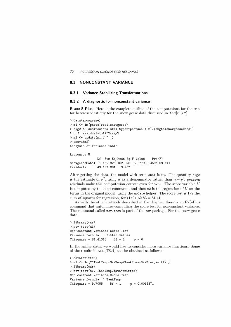
72 REGRESSION DIAGNOSTICS: RESIDUALS
8.3 NONCONSTANT VARIANCE
8.3.1 Variance Stabilizing Transformations
8.3.2 A diagnostic for nonconstant variance
R and S-Plus Here is the complete outline of the computations for the testfor heteroscedasticity for the snow geese data discussed in alr[8.3.2]:
> data(snowgeese)
> m1 <- lm(photo~obs1,snowgeese)
> sig2 <- sum(residuals(m1,type="pearson")^2)/length(snowgeese$obs1)
> U <- residuals(m1)^2/sig2
> m2 <- update(m1,U ~ .)
> anova(m2)
Analysis of Variance Table
Response: U
Df Sum Sq Mean Sq F value Pr(>F)
snowgeese$obs1 1 162.826 162.826 50.779 8.459e-09 ***
Residuals 43 137.881 3.207
After getting the data, the model with term obs1 is fit. The quantity sig2
is the estimate of σ2, using n as a denominator rather than n − p′. pearson
residuals make this computation correct even for wls. The score variable Uis computed by the next command, and then m2 is the regression of U on theterms in the original model, using the update helper. The score test is 1/2 thesum of squares for regression, for (1/2)162.83 = 81.41.
As with the other methods described in the chapter, there is an R/S-Pluscommand that automates computing the score test for nonconstant variance.The command called ncv.test is part of the car package. For the snow geesedata,
> library(car)
> ncv.test(m1)
Non-constant Variance Score Test
Variance formula: ~ fitted.values
Chisquare = 81.41318 Df = 1 p = 0
In the sniffer data, we would like to consider more variance functions. Someof the results in alr[T8.4] can be obtained as follows:
> data(sniffer)
> m1 <- lm(Y~TankTemp+GasTemp+TankPres+GasPres,sniffer)
> library(car)
> ncv.test(m1,~TankTemp,data=sniffer)
Non-constant Variance Score Test
Variance formula: ~ TankTemp
Chisquare = 9.7055 Df = 1 p = 0.0018371

GRAPHS FOR MODEL ASSESSMENT 73
> ncv.test(m1,~TankTemp+GasPres,data=sniffer)
Non-constant Variance Score Test
Variance formula: ~ TankTemp + GasPres
Chisquare = 11.778 Df = 2 p = 0.0027695
> ncv.test(m1,~TankTemp+GasTemp+TankPres+GasPres,data=sniffer)
Non-constant Variance Score Test
Variance formula: ~ TankTemp + GasTemp + TankPres + GasPres
Chisquare = 13.76 Df = 4 p = 0.008102
> ncv.test(m1)
Non-constant Variance Score Test
Variance formula: ~ fitted.values
Chisquare = 4.8027 Df = 1 p = 0.028416
To use ncv.test, specify the regression model, then a one-sided formula thatspecifies the model for the variance, and then if necessary the data frame.
8.3.3 Additional comments
8.4 GRAPHS FOR MODEL ASSESSMENT
8.4.1 Checking mean functions
R and S-Plus The alr3 package has two commands for drawing marginalmodel plots; mmp draws one marginal model plot, while mmps draws many suchplots.
alr[F8.11] is created by
> data(ufcwc)
> c1 <- lm(Height~Dbh,ufcwc)
> mmp(c1,ufcwc$Dbh,label="Diameter, Dbh",color=c("blue","red"))
The first argument to mmp is the only required argument, and is the nameof a regression model. The second argument is the quantity to put on thehorizontal axis of the plot, with predict(c1) as the default. We have showntwo additiona arguments, for the horizontal axis label and the colors of thetwo smooths; neither argument is required.
The command mmp uses the loess smoother, with defaults degree=1, span=2/3;both of these values can be changed when using the command. An interestingexercise would be to implement marginal model plots with other smoothers,and with non-deterministic methods for selecting a bandwidth parameter.
To draw marginal model plots versus each predictor and versus fitted val-ues, use mmps. The following will draw three of the four plots in alr[F8.13]:
> m1 <- lm(logFertility~logPPgdp+Purban,UN2)
> mmps(m1)

74 REGRESSION DIAGNOSTICS: RESIDUALS
The fourth plot in alr[F8.13] plots in a direction that is a random lin-ear combination of the terms. You can get plots like this one using therandom.lin.comb command in the alr3 package,
> mmps(m1,u=random.lin.comb(m1))
Every time you draw this last plot, it will be different because the randomnumbers used will change. If you want to reproduce a plot, use the seed
argument:
> mmps(m1,u=random.lin.comb(m1,seed=254346576))
8.4.2 Checking variance functions
R and S-Plus The commands mmp and mmps include an argument sd that ifset to TRUE will add the standard deviation smooths to the plot, as describedin alr[8.4.2].

9Outliers and Influence
9.1 OUTLIERS
9.1.1 An outlier test
R and S-Plus In R or using the car library in S-Plus, the command rstandard
computes the standardized residuals alr[E9.3]. You can also use alr[E9.3]to compute these directly. Given a model m1,
> # For R only:
> ri <- residuals(m1,type="pearson")/(sigma.hat(m1)*
sqrt(1-hatvalues(m1))
> # For S-Plus only
> ri <- residuals(m1,type="pearson")/(sigma.hat(m1)*
sqrt(1-lm.influence(m1)$hat)
Pearson residuals guarantee that the same formula will work with weightedor unweighted least squares.
The outlier test is computed in R or with the car library in S-Plus usingrstudent. These, too, can be computed directly. For a model m1, we usealr[E9.4],
> ti <- ri* sqrt((m1$df-1)/(m1$df-ri^2))
The quantity m1$df is the df for residuals, equal to n− p′.
75

76 OUTLIERS AND INFLUENCE
9.1.2 Weighted least squares
9.1.3 Significance levels for the outlier test
R and S-Plus Significance levels for the outlier test use the pt command.For example, if the largest in absolute value of n = 65 Studentized residualsis 2.85, with p′ = 5, the df for error is n − p′ − 1 = 65 − 5 − 1 = 59. Thesignificance level, using the Bonferroni bound, is
> 65*2*(1-pt(2.85,59))
[1] 0.39084
By subracting the result of the pt command from one, we get the upper tail,rather than the lower tail. We multiply by two to get a two-tailed test. Wemultiply by n = 65 for the Bonferroni inequality.
If you have a regression model m, the test for one outlier is1
> n*2*(1-pt(max(abs(rstudent(m)),m$df-1))
You can find the case number of the maximum Studentized residual with
> match(max(abs(rstudent(m))),abs(rstudent(m)))
9.1.4 Additional comments
9.2 INFLUENCE OF CASES
R and S-Plus Table 8.1 lists the fundamental commands for influence andoutlier statistics. Each of the commands returns a vector.
In addition, R and S-Plus will compute and return the building blocksthat are used in computing these statistics. In particular, the commandinfluence in R, called lm.influence in S-Plus, returns a structure of thesebuilding blocks. For example, if you have a model m1, then type
> ans <- influence(m1)
ans$coefficients returns a matrix with n rows and p′ columns whose ithrow is β(i), alr[E9.5]. This latter quantity was used to draw alr[F9.1].ans$sigma returns a vector of the σ(i), the square roots of the estimate of σ,each computed with one case deleted. Finally, ans$hat returns the leverage.In linear models, all the leave-one-out statistics can be computed from theleverages and residuals, so neither of the first two quantities are computed inan influence analysis.
R and S-Plus make refitting a regression with one (or a few) cases deletedeasy. Suppose your model m1 was fit with n = 96 cases, and you want to refit,leaving out cases 2, 7, 16. You need only type
1Reminder: rstudent is available in the base R, but for S-Plusyou need to load the librarycar.

NORMALITY ASSUMPTION 77
> m2 <- update(m1, subset=(1:96)[-c(2,7,16)])
which uses the subset argument to update to refit with the specified casesdeleted. The value of the subset argument can be either a vector of casenumbers, as is the case here, or a vector of logical values with TRUE for valuesto be included, and FALSE for values to be excluded.
9.2.1 Cook’s distance
R and S-Plus The command cooks.distance in R and in the car libraryfor S-Plus computes Cook’s distance. It can also be computed directly fromalr[E9.8] for a model m1,
> # For R only
> Di <- (ri^2/m1$rank)* (hatvalues(m1))/(1-hatvalues(m1))
> # For S-Plus only
> Di <- (ri^2/m1$rank)*(lm.influence(m1)$hat)/(1-lm.influence(m1)$hat)
m1$rank counts up the number of coefficients estimated in the mean function,so it is equal to p′.
9.2.2 Magnitude of Di
R and S-Plus The command inf.index in the alr3 package is used to drawindex plots of diagnostic statistics, like alr[F9.3]. Here are the commandsto draw this figure:
> data(rat)
> m1 <- lm(y~BodyWt+LiverWt+Dose,rat)
> inf.index(m1)
This function also gives an index plot of the p-values for the (two-tailed)outlier test based on the Bonferroni inequality.
9.2.3 Computing Di
9.2.4 Other measures of influence
R and S-Plus Just a reminder: added-variable plots are available in the car
package; see Section 3.1.
9.3 NORMALITY ASSUMPTION
R and S-Plus The qqnorm command is used to draw normal probability plots.Here are the commands to draw alr[F9.5], which shows two normal proba-bility plots.
> data(heights)

78 OUTLIERS AND INFLUENCE
> m1 <- lm(Dheight ~ Mheight, heights)
> data(transact)
> t1 <- lm(Time~T1+T2,transact)
> par(mfrow=c(1,2),mar=c(4,3,0,.5)+.1,mgp=c(2,1,0),cex=.5)
> qqnorm(residuals(m1),xlab="(a) Heights data",main="")
> qqnorm(residuals(t1),xlab="(a) Transaction data",main="")

10Variable Selection
10.1 THE ACTIVE TERMS
The first example in this chapter uses randomly generated data. This can behelpful in trying to understand issues against a background where we knowthe right answers. Generating random data is possible in most statisticalpackages, though doing so may not be easy or intuitive.
R and S-Plus Here is code in R for generating the random data with standardnormal random variables, and then fitting the regression for the first case inalr[10.1]
> case1 <- data.frame(x1=rnorm(100),x2=rnorm(100),
+ x3=rnorm(100),x4=rnorm(100))
> e <- rnorm(100)
> case1$y <- 1 + case1$x1 + case1$x2 + e
> m1 <- lm(y~x1+x2+x3+x4,data=case1)
The data.frame command created a data frame, with each variable consistingof 100 standard normal pseudo-random numbers. The variable case1$y wasadded to the data frame to be the response, and then the model was fit.
Case 2 is more complicated because the random predictors are correlated.We use the result alr[EA.18]. If X is an n×pmatrix whose rows are normallydistributed with identity covariance matrix, then for any p× p matrix S, thethe matrix Z = XS has rows with variance S(S)′. In our application, let S
79

80 VARIABLE SELECTION
be any matrix such that
Var(X2) = S(S)′ =
1 0 .95 00 1 0 −.95.95 0 1 00 −.95 0 1
where the right side of this equation is from alr[E10.2]. Any matrix S thatsatisfies this equation is called a square root of Var(X2). The square root isnot unique. If we can find such an S, then the matrix XS will have rows thatare normally distributed with the desired covariance matrix.
Here is the computation in R:
> X <- as.matrix(case1[,-5]) # change from data.frame to a matrix, drop y
> Var2 <- matrix(c(1, 0, .95, 0,
+ 0, 1, 0,-.95,
+ .95, 0, 1, 0,
+ 0,-.95, 0, 1), ncol=4)
> s1 <- chol(Var2) # cholesky factor of Var2
> X <- X %*% s1
> dimnames(X)[[2]] <- c("x1","x2","x3","x4")
> case2 <- data.frame(X)
> case2$y <- 1 + case2$x1 + case2$x2 + e
> m2 <- lm(y~x1+x2+x3+x4,data=case2)
We begin by converting case1 from a data frame to a matrix, and dropping thevariable for the response; R does not allow matrix operations on data frames.Then, we define Var2 according to alr[E10.2]. The matrix S can be anysquare root of Var2, and we have used the Cholesky factorization computedby chol. The next line computes the new predictors with the right covariancematrix. dimnames restores the variable names, and then we procede as before.We have used the same random numbers for the two cases, which will makethe results correlated. If we had used different random numbers, the resultsof fitting the two cases would be uncorrelated.
10.1.1 Collinearity
R and S-Plus The variance inflation factors, defined following alr[E10.5],are computed by the command vif in the car package. Here are the varianceinflation factors for the first two examples in alr[10.1]
> vif(m1)
x1 x2 x3 x4
1.0072 1.0379 1.0330 1.0082
> vif(m2)
x1 x2 x3 x4
14.973 16.421 15.057 16.389
As expected, in the first case the variance inflation factors are all close to one,but in the second example they are all large.

VARIABLE SELECTION 81
10.1.2 Collinearity and variances
10.2 VARIABLE SELECTION
10.2.1 Information criteria
The information criteria alr[E10.7]–alr[E10.9] depend only on the RSS,p′, and possibly an estimate of σ2, and so if these are needed for a particularmodel, they can be computed from the usual summaries available in a fittedregression model.
R In R only, there is a command extractAIC that can be used to computeAIC, BIC and Cp. For a fitted subset model m0 and a fitted larger model m1,the following commands extract these quantities:
> extractAIC(m0,k=2) # give AIC
> extractAIC(m0,k=log(length(m0$residuals)) # gives BIC
> extractAIC(m0,scale=sigma.hat(m1)^2) # gives Cp
10.2.2 Computationally intensive criteria
Computation of PRESS, alr[E10.10], is not common in regression programs,but it is easy to obtain given the residuals and leverages from a fitted model.
R and S-Plus In R and S-Plus, given a model m1, PRESS can be computedas
> PRESS <- sum((residuals(m1,type="pearson")/(1-ls.diag(m1)$hat))^2)
This simple computation works for linear models, but not for more complexmodels such as nonlinear or generalized linear models.
10.2.3 Using subject-matter knowledge
10.3 COMPUTATIONAL METHODS
R and S-Plus Four basic commands are included for use when examiningmany possible regression models, as listed in Table 10.1.
The primary command we recommend using is step. Using the highwaydata in alr[T10.5], we start by fitting the largest and smallest models thatwe want to consider:
> m1 <- lm(logRate ~ logLen+logADT+logTrks+logSigs1+Slim+Shld+
+ Lane+Acpt+Itg+Lwid+Hwy, data=highway)
> m0 <- lm(logRate ~logLen,data=highway)
As discussed in alr[10.2.1], log(Len) will be in all subsets. One of the terms,Hwy, is a factor with 3 df. Here is the command for fitting via forwardselection:

82 VARIABLE SELECTION
Table 10.1 R/S-Plus commands relating to subset selection.
Fit all possible subsets and find the best few
leaps Uses the Furnival and Wilson algorithm to examine all possible regres-sions. In R, you must obtain and load the package leaps. The syntaxof this command is different from the rest of R and S-Plus. You mustspecify the predictors in a matrix, and the response in a separate vector;factors are not permitted. The output from the command is confusing,and selection can only be based on Cp, not on the other informationcriteria. Serious use of this function will require writing a command toprocess the output in an intelligent manner.
regsubsets Part of the leaps package for R, and not available in S-Plus, this com-mand purports to improve on leaps, but the documentation is unclear,and the output is still confusing.
stepwise Available only in S-Plus, this command uses a brute force algorithm toexamine all possible subset mean functions, and return the few withthe smallest value of Cp. The method does not permit other criteria,or correctly handle factors. In addition, data must be supplied as inleaps in the form of a matrix and a vector rather than as a formulaand a data frame.
Functions based on stepwise selection
step Use this function for both forward selection, backward elimination, ora combination of them, based on any of the information criteria exceptfor PRESS.
drop1 This command will fit all models obtained by a current fitted modelby dropping one term, and gives very easy to interpret output. Withthis command, you can do backward elimination “by hand,” one stepat a time. This is particularly helpful in problems with factors andinteractions, since dropping a main effect from a mean function thatincludes interactions with that variable is not recommended.
add1 Adds one term from a potential pool of terms to the fitted model. Thiscan be used for forward selection “by hand.”

COMPUTATIONAL METHODS 83
> ansf1 <- step(m0,scope=list(lower=~logLen,
+ upper=~logLen+logADT+logTrks+logSigs1+Slim+Shld+
+ Lane+Acpt+Itg+Lwid+Hwy),
+ direction="forward", data=highway)
The first argument to step is the name of a model, and for forward selection, itis the smallest model considered. The argument scope gives explicity the thelower and upper models, via one-sided formulas. The direction is specifiedin quotation marks, and then the data frame must be named. The output ofthis command is very long:
Start: AIC= -43.92
logRate ~ logLen
Df Sum of Sq RSS AIC
+ Slim 1 5.3 6.1 -66.3
+ Acpt 1 4.4 7.0 -60.8
+ Shld 1 3.6 7.9 -56.5
+ logSigs1 1 2.0 9.4 -49.4
+ Hwy 3 2.8 8.6 -48.8
+ logTrks 1 1.5 9.9 -47.5 Step 1
+ logADT 1 0.9 10.5 -45.1
<none> 11.4 -43.9
+ Lane 1 0.5 10.9 -43.8
+ Itg 1 0.5 11.0 -43.5
+ Lwid 1 0.4 11.0 -43.3
Step: AIC= -66.28
logRate ~ logLen + Slim
Df Sum of Sq RSS AIC
+ Acpt 1 0.6 5.5 -68.3
+ logTrks 1 0.5 5.6 -67.9
<none> 6.1 -66.3
+ logSigs1 1 0.3 5.8 -66.3
+ Hwy 3 0.7 5.4 -65.0 Step 2
+ Shld 1 0.1 6.0 -64.7
+ logADT 1 0.1 6.1 -64.6
+ Lwid 1 0.0346 6.1 -64.5
+ Lane 1 0.0071 6.1 -64.3
+ Itg 1 0.0055 6.1 -64.3
Step: AIC= -68.31
logRate ~ logLen + Slim + Acpt
Df Sum of Sq RSS AIC
+ logTrks 1 0.4 5.2 -68.9
<none> 5.5 -68.3
+ logSigs1 1 0.2 5.3 -68.1
+ Shld 1 0.1 5.4 -66.8

84 VARIABLE SELECTION
+ logADT 1 0.032 5.5 -66.5 Step 3
+ Lane 1 0.031 5.5 -66.5
+ Itg 1 0.028 5.5 -66.5
+ Lwid 1 0.026 5.5 -66.5
+ Hwy 3 0.5 5.1 -65.7
Step: AIC= -68.94
logRate ~ logLen + Slim + Acpt + logTrks
Df Sum of Sq RSS AIC
<none> 5.2 -68.9
+ Shld 1 0.1 5.0 -68.0
+ logSigs1 1 0.1 5.0 -67.7
+ logADT 1 0.1 5.1 -67.4
+ Hwy 3 0.5 4.6 -67.3 Step 4
+ Lwid 1 0.0396 5.1 -67.2
+ Itg 1 0.0228 5.1 -67.1
+ Lane 1 0.0069 5.1 -67.0
The default criterion for fitting is AIC. The output marked Step 1 gives thesummary for each mean function obtained by adding one term to the basemodel given by m0. The models are ordered, so the one that minimizes AICappears first.
At Step 2, Slim is added to the current model, and all the mean functionsadd one term to log(Len) and Slim. Steps continue until the model at theprevious step, marked <none> has smaller AIC than adding the next term; inthis example this occurs at Step 4, so the base model for this step is takenas the minimizer of AIC. The object ansf1 is the fitted model that minimizesAIC.
In S-Plus, step works similarly, but the default information criterion is Cp
rather than AIC.Backward elimination is similar, except the specified model is the largest
one.
> ansf2 <- step(m1,scope=list(lower=~logLen,
+ upper=~logLen+logADT+logTrks+logSigs1+Slim+Shld+
+ Lane+Acpt+Itg+Lwid+Hwy),
+ direction="backward", data=highway,
+ scale=sigma.hat(m1)^2)
The other arguments are similar to the arguments for forward selection. Inthis example, we have set scale=sigma.hat(m1)^2, in which case the selectioncriterion is Cp, not AIC. If you set k=log(length(residuals$m1)), then BICwill be used. You can’t use PRESS with this command. Here is the output:
Start: AIC= 14
logRate ~ logLen + logADT + logTrks + logSigs1 + Slim + Shld +
Lane + Acpt + Itg + Lwid + Hwy

COMPUTATIONAL METHODS 85
Df Sum of Sq RSS Cp
- Shld 1 0.0011 3.54 12.0
- Itg 1 0.0031 3.54 12.0
- Lane 1 0.01 3.54 12.0
- Lwid 1 0.01 3.55 12.1
- Hwy 3 0.63 4.16 12.4
- Acpt 1 0.08 3.62 12.6
- logTrks 1 0.10 3.63 12.7
- logADT 1 0.27 3.81 13.9
<none> 3.54 14.0
- Slim 1 0.37 3.91 14.6
- logSigs1 1 0.92 4.46 18.5
Step: AIC= 12.01
logRate ~ logLen + logADT + logTrks + logSigs1 + Slim + Lane +
Acpt + Itg + Lwid + Hwy
Df Sum of Sq RSS Cp
- Itg 1 0.0028 3.54 10.0
- Lane 1 0.01 3.54 10.1
- Lwid 1 0.01 3.55 10.1
- Acpt 1 0.10 3.64 10.7
- logTrks 1 0.12 3.65 10.8
- Hwy 3 0.68 4.22 10.8
<none> 3.54 12.0
- logADT 1 0.28 3.82 12.0
- Slim 1 0.71 4.25 15.0
- logSigs1 1 1.00 4.54 17.1
Step: AIC= 10.03
logRate ~ logLen + logADT + logTrks + logSigs1 + Slim + Lane +
Acpt + Lwid + Hwy
Df Sum of Sq RSS Cp
- Lane 1 0.01 3.55 8.06
- Lwid 1 0.01 3.55 8.13
- Acpt 1 0.09 3.64 8.70
- logTrks 1 0.12 3.66 8.86
<none> 3.54 10.03
- logADT 1 0.32 3.86 10.31
- Hwy 3 1.16 4.71 12.26
- Slim 1 0.79 4.33 13.61
- logSigs1 1 1.00 4.54 15.11
Step: AIC= 8.06
logRate ~ logLen + logADT + logTrks + logSigs1 + Slim + Acpt +
Lwid + Hwy
Df Sum of Sq RSS Cp

86 VARIABLE SELECTION
- Lwid 1 0.02 3.56 6.18
- Acpt 1 0.10 3.64 6.75
- logTrks 1 0.11 3.66 6.87
<none> 3.55 8.06
- logADT 1 0.38 3.93 8.76
- Hwy 3 1.28 4.82 11.08
- Slim 1 0.80 4.35 11.72
- logSigs1 1 1.02 4.56 13.26
Step: AIC= 6.18
logRate ~ logLen + logADT + logTrks + logSigs1 + Slim + Acpt +
Hwy
Df Sum of Sq RSS Cp
- Acpt 1 0.10 3.67 4.92
- logTrks 1 0.13 3.69 5.09
<none> 3.56 6.18
- logADT 1 0.37 3.93 6.77
- Hwy 3 1.27 4.84 9.18
- Slim 1 0.80 4.36 9.81
- logSigs1 1 1.03 4.59 11.46
Step: AIC= 4.92
logRate ~ logLen + logADT + logTrks + logSigs1 + Slim + Hwy
Df Sum of Sq RSS Cp
- logTrks 1 0.14 3.81 3.93
<none> 3.67 4.92
- logADT 1 0.31 3.98 5.11
- Hwy 3 1.51 5.18 9.61
- logSigs1 1 1.16 4.83 11.12
- Slim 1 1.21 4.87 11.45
Step: AIC= 3.93
logRate ~ logLen + logADT + logSigs1 + Slim + Hwy
Df Sum of Sq RSS Cp
<none> 3.81 3.93
- logADT 1 0.29 4.10 3.96
- Hwy 3 1.69 5.50 9.84
- Slim 1 1.16 4.97 10.12
- logSigs1 1 1.56 5.37 12.98
The commands drop1 and add1 do one step of these methods, so you can dothe stepwise fitted “by hand.”

WINDMILLS 87
10.3.1 Subset selection overstates significance
10.4 WINDMILLS
10.4.1 Six mean functions
10.4.2 A computationally intensive approach
The data for the windmill example in alr[10.4.2] is not included with thealr3 library, and must be downloaded separately from www.stat.umn.edu/alr.The R or S-Plus commands used to compute alr[F10.1] are given in the scriptfor this chapter. The process requires many statements, but the method isstraightforward. The command to compute the simulation in the script for thischapter has a comment marker in front of it, as the simulation can take severalhours to complete. The results from the simulation discussed in alr[10.4.2]are available from the data page at www.stat.umn.edu/alr in the file sim1.out.


11Nonlinear Regression
11.1 ESTIMATION FOR NONLINEAR MEAN FUNCTIONS
11.2 INFERENCE ASSUMING LARGE SAMPLES
R and S-Plus The command nls is used to obtain ols and wls estimatesfor nonlinear regression models. nls differs from lm in a few key respects:
1. The formula for defining a model is different. In lm, a typical formulais Y∼X1+X2+X3+X4. This formula specifies the names of the response andthe terms, but not the names of the parameters because to each termthere is an associated parameter, or parameters for a factor. For anls model, the formula specifies both terms and parameters. A typicalexample might be Y∼th1 + th2*(1-exp(-th3*x)). In this case there arethree parameters, th1, th2 and th3, but only one term, x. The right-hand side formula should be an expression of parameters, terms, andnumbers that can be evaluated by the computer language C.
2. Factors are generally not used with nls.
3. A named list start of starting values must be specified. This serves thedual purpose of telling the algorithm where to start, and also to namethe parameters. For the example, start=list(th1=620,th2=200,th3=10)indicates that th1, th2 and th3 are parameters, and so by implicationthe remaining quantity, x, must be a predictor variable.
89

90 NONLINEAR REGRESSION
4. Most iterative algorithms for nonlinear least squares require compu-tation of derivatives, and many programs require the user to provideformulas for the derivatives. This is not the case in nls; all derivativesare computed using numerical differentiation.
Here is the input leading to alr[T11.2]
> data(turk0) # R only
> n1 <- nls(Gain ~ th1 + th2*(1-exp(-th3*A)), data=turk0,
start=list(th1=620,th2=200,th3=10))
> summary(n1)
Formula: Gain ~ th1 + th2 * (1 - exp(-th3 * A))
Parameters:
Estimate Std. Error t value Pr(>|t|)
th1 622.96 5.90 105.57 < 2e-16
th2 178.25 11.64 15.32 2.7e-16
th3 7.12 1.21 5.91 1.4e-06
Residual standard error: 19.7 on 32 degrees of freedom
Correlation of Parameter Estimates:
th1 th2
th2 -0.312
th3 -0.406 -0.62
After loading the data, we called nls with the required arguments of a for-mula and starting values. In addition, we specified a data frame. In R, thereare many other arguments to nls, including several that are identical witharguments of the same name in lm, including subset for selecting cases, andna.action for setting the missing value action; neither of these is available inS-Plus. A few arguments are used to change the details of the computing algo-rithm; see the help page for nls. Neither R nor S-Plus have a weights argumentfor fitting wls1, but see the next example for computing wls estimates.
The printed output from the summary method is also similar to the outputfrom ls, as described in alr[11.2]. The “correlation of parameter estimates”is the matrix alr[E11.14] rescaled as a correlation matrix.
Similar to an object created by the lm command, objects created by nls
have summary, plot and predict methods, and these are used in a way that issimilar to linear regression models. For example, alr[F11.2] is obtained by
> attach(turk0)
> plot(A,Gain, xlab="Amount (percent of diet)", ylab="Weight gain, g")
> x <- (0:44)/100
> lines(x,predict(n1,data.frame(A=x)))
1The argument exists in R but as of October 2004 it has not been implemented.

INFERENCE ASSUMING LARGE SAMPLES 91
Lack-of-fit testing is possible if there are repeated observations. The ideais to compare the nonlinear fit to the one-way analysis of variance, using thelevels of the predictor as a grouping variable:
> m1 <- lm(Gain~as.factor(A),turk0)
> anova(n1,m1)
Analysis of Variance Table
Model 1: Gain ~ th1 + th2 * (1 - exp(-th3 * A))
Model 2: Gain ~ as.factor(A)
Res.Df Res.Sum Sq Df Sum Sq F value Pr(>F)
1 32 12367
2 29 9824 3 2544 2.5 0.079
The model m1 is a linear model, while n1 is a nonlinear model. Even so, theanova will correctly compare them, giving the F test for lack of fit.
Unlike lm, nls does not allow factors in a formula. To use factors, you needto create dummy variables for the various levels of the factor and use these.
For example, consider fitting the models alr[11.17]–alr[11.19]. The dataframe turkey includes a variable S that is a factor with three levels for thesource of the dietary addtive. Weighted least squares is required. We canapply alr[E5.8] to get nls to get wls estimates. We have y = g(θ, x)+e/
√w
where the e’s have constant variance, so the y’s have variance σ2/w. Multiplyboth sides of the mean function by
√w to get
√wy =
√wg(θ, x) + e so we
can get wls estimates in the original problem by getting ols estimates with√wg(θ, x) as the kernel mean function, and
√wy as the response.
The code for fitting the four models using wls is given next. The vectorm is the number of pens at each treatment combination, and is the vector ofweights for this problem, S is the factor, and Gain is the response variable.
data(turkey) # R only
tdata <- turkey # copy data to local name, requires only for Splus
# create the indicators for the categories of S
tdata$S1 <- tdata$S2 <- tdata$S3 <- rep(0,dim(tdata)[1])
tdata$S1[tdata$S==1] <- 1
tdata$S2[tdata$S==2] <- 1
tdata$S3[tdata$S==3] <- 1
# compute the weighted response
tdata$wGain <- sqrt(tdata$m)*tdata$Gain
# fit the models
# common regressions
m4 <- nls( wGain ~ sqrt(m)*(th1 + th2*(1-exp(-th3*A))),
data=tdata,start=list(th1=620,th2=200,th3=10))
# most general
m1 <- nls( wGain ~ sqrt(m)*(S1*(th11 + th21*(1-exp(-th31*A)))+
S2*(th12 + th22*(1-exp(-th32*A)))+
S3*(th13 + th23*(1-exp(-th33*A)))),
data=tdata,start= list(th11=620,th12=620,th13=620,
th21=200,th22=200,th23=200,

92 NONLINEAR REGRESSION
th31=10,th32=10,th33=10))
# common intercept
m2 <- nls(wGain ~ sqrt(m)*(th1 +
S1*(th21*(1-exp(-th31*A)))+
S2*(th22*(1-exp(-th32*A)))+
S3*(th23*(1-exp(-th33*A)))),
data=tdata,start= list(th1=620,
th21=200,th22=200,th23=200,
th31=10,th32=10,th33=10))
# common intercept and asymptote
m3 <- nls( wGain ~ sqrt(m)*(th1 + th2 *(
S1*(1-exp(-th31*A))+
S2*(1-exp(-th32*A))+
S3*(1-exp(-th33*A)))),
data=tdata,start= list(th1=620, th2=200,
th31=10,th32=10,th33=10))
We have now created the dummy variables, weighted response, and the modelswith different mean functions. If there were no weights, we could leave off thesqrt(w) in the above statements, and use Gain, not wGain, as the response. Ineach of the models we had to specify starting values for all the parameters.The starting values we use essentially assume no group differences. Here arethe anova tables to compare the models:
> anova(m4,m2,m1)
Analysis of Variance Table
Model 1: wGain ~ sqrt(m) * (th1 + th2 * (1 - exp(-th3 * A)))
Model 2: wGain ~ sqrt(m) * (th1 + S1 * (th21 * (1 - exp(-th31 * A)))
+ S2 * (th22 * (1 - exp(-th32 * A)))
+ S3 * (th23 * (1 - exp(-th33 * A))))
Model 3: wGain ~ sqrt(m) * (S1 * (th11 + th21 * (1 - exp(-th31 * A)))
+ S2 * (th12 + th22 * (1 - exp(-th32 * A)))
+ S3 * (th13 + th23 * (1 - exp(-th33 * A))))
Res.Df Res.Sum Sq Df Sum Sq F value Pr(>F)
1 10 4326
2 6 2040 4 2286 1.68 0.27
3 4 1151 2 889 1.54 0.32
> anova(m4,m3,m1)
Analysis of Variance Table
Model 1: wGain ~ sqrt(m) * (th1 + th2 * (1 - exp(-th3 * A)))
Model 2: wGain ~ sqrt(m) * (th1 + th2 * (S1 * (1 - exp(-th31 * A))
+ S2 * (1 - exp(-th32 * A)) + S3 * (1 - exp(-th33 * A))))
Model 3: wGain ~ sqrt(m) * (S1 * (th11 + th21 * (1 - exp(-th31 * A)))
+ S2 * (th12 + th22 * (1 - exp(-th32 * A)))
+ S3 * (th13 + th23 * (1 - exp(-th33 * A))))
Res.Df Res.Sum Sq Df Sum Sq F value Pr(>F)
1 10 4326
2 8 2568 2 1758 2.74 0.12

BOOTSTRAP INFERENCE 93
3 4 1151 4 1417 1.23 0.42
These tests are interpreted as in alr[6.2.2].
11.3 BOOTSTRAP INFERENCE
R The bootstrap be done using the same boot.case command used for linearmodels. For example, to get the bootstrap leading to alr[F11.5], using R
> data(segreg) # R only
> attach(segreg)
> smod <- C ~ th0 + th1*(pmax(0,Temp-gamma))
> s1 <- nls(smod, data=segreg,start=list(th0=70,th1=.5,gamma=40))
> set.seed(10131985)
> s1.boot <- boot.case(s1,B=999)
If you are using S-Plus, load the package resample and replace the call toboot.case by bootstrap(s1,coef,B=999). By using the set.seed command inR, you will get exactly the same bootstrap replications discussed in alr; leavethis command off, or change the seed, and you will get different replications.
s1.boot will consist only of a matrix with 999 rows and 3 columns, one rowfor each replication, and one column for each parameter, and summarizingthe bootstrap is your responsibility. The summary used in alr uses thescatterplot.matrix command in the car package2
> library(car)
> scatterplot.matrix(s1.boot,diagonal="histogram",
+ col=palette(),#[-1],
+ lwd=0.7,pch=".",
+ labels=c(expression(theta[1]),expression(theta[2]),
+ expression(gamma)),
+ ellipse=FALSE,smooth=TRUE,level=c(.90))
Numerical summaries can also be appropriate, for example,
> s1.boot.summary <- data.frame(rbind(
+ apply(s1.boot,2,mean),
+ apply(s1.boot,2,sd),
+ apply(s1.boot,2,function(x){quantile(x,c(.025,.975))})))
> row.names(s1.boot.summary)<-c("Mean","SD","2.5%","97.5%")
> s1.boot.summary
th0 th1 gamma
Mean 74.8407 0.60701 43.1235
SD 1.4453 0.11833 4.6156
2.5% 72.0214 0.46359 36.8698
97.5% 77.5957 0.97129 55.0744
2scatterplot.matrix is not available in S-Plus. Use pairs instead.

94 NONLINEAR REGRESSION
Here we combined the summaries into a data frame so they would be prettywhen printed. The apply command is used repeatedly to apply functionsto the columns of s1.boot, and we summarize with the mean, SD, and 95%percentile-based confidence interval for each parameter.
S-Plus Bootstrapping nonlinear models is not straightforward in S-Plus, andneither the boot.case command in the alr3 package, nor the bootstrap com-mand in the resample library work for nonlinear model objects. The heartof the problem is that nls in S-Plus does not accept the subset argument, sopermuting cases as is required in bootstrapping is relatively difficult. If youwrite S-Plus code for bootstrapping a nonlinear model, let us know and wewill add it to the alr3 library.
11.4 REFERENCES

12Logistic Regression
Both logistic regression and the normal linear models that we have discussedin earlier chapters are examples of generalized linear models. Many programs,including SAS, R, and S-Plus, have procedures that can be applied to anygeneralized linear model. Both JMP and SPSS seem to have separate pro-cedures for logistic regression. There is a possible source of confusion in thename. Both SPSS and SAS use the name general linear model to indicate arelatively complex linear model, possibly with continuous terms, covariates,interactions, and possibly even random effects, but with normal errors. Thusthe general linear model is a special case of the generalized linear models.
12.1 BINOMIAL REGRESSION
12.1.1 Mean Functions for Binomial Regression
12.2 FITTING LOGISTIC REGRESSION
R and S-Plus The key command in fitting a generalized linear model is glm.We will only consider the logistic regression case, but only minor changes arerequired for other cases.
Here is a general form for the glm command, illustrating the basic argu-ments available for binomial regression:
glm(formula, family = binomial(link="logit"), data, weights,
subset, na.action, start = NULL)
95

96 LOGISTIC REGRESSION
The arguments data, weights, subset and na.action are used in the same waythey are used in lm. The family argument is new, and the formula argumentis a little different than its use in lm or nls. There are a few other arguments,mostly modifying the computational algorithm, that will probably be rarelyneeded.
As in alr[12.1.1], let θ(x) be the probability of success given the value ofthe terms X in the mean function equal x. According to the logistic regressionmodel, we have from alr[E12.7]
log
(
θ(x)
1 − θ(x)
)
= β′x (12.1)
The quantity on the right of this equation is called the linear predictor. Thequantity on the left depends on the link function (or equivalently, the kernelmean function) used in fitting, which in this case is the logit link, the inverseof the logistic kernel mean function discussed in alr[10.1.1].
The formula for a glm is a two-sided formula. The right-hand side of thisformula is the linear predictor, equivalent to β′x in (12.1). The left-hand sideis either: (1) if the number of trials is always equal to one for each case, thenthe left-hand side is just the the response variable, a vector of zeroes and ones.(2) If the number of trials is not always equal to one, then the left-hand sideis a matrix with two columns, the first column giving the number of successesand the second giving the number of failures.
The family argument is the name of an error distribution, which is binomialfor binomial regression. Other choices like Poisson and gaussian are used forPoisson errors and normal errors, respectively. As an argument to the family,you set the link function. The only link discussed in alr is the logit linkfor logistic regression. Since this is the default, it need not be specified. Seevr[7] for a more general discussion.
12.2.1 One-predictor example
R and S-Plus For alr[T12.1], here are the computations:
> data(blowBF)
> m1 <- glm(y~logb(D,2),family=binomial(),data=blowBF)
> summary(m1)
Call:
glm(formula = y ~ logb(D, 2), family = binomial(), data = blowBF)
Deviance Residuals:
Min 1Q Median 3Q Max
-2.507 -0.757 -0.494 0.810 2.327
Coefficients:
Estimate Std. Error z value Pr(>|z|)

FITTING LOGISTIC REGRESSION 97
(Intercept) -7.892 0.633 -12.5 <2e-16
logb(D, 2) 2.263 0.191 11.8 <2e-16
(Dispersion parameter for binomial family taken to be 1)
Null deviance: 856.21 on 658 degrees of freedom
Residual deviance: 655.24 on 657 degrees of freedom AIC: 659.2
The linear predictor used consists of the base-two logarithm of D. The family
must be specified, because the default is family=gaussian, but the link can beskipped because the default is "logit".
Here are the commands to draw alr[F12.1a].
> plot(jitter(logb(D,2),amount=.05),
+ jitter(y,amount=0.02),
+ xlab=expression(paste("(a) ",Log[2](Diameter))),
+ ylab="Blowdown indicator")
> xx <- seq(min(D),max(D),length=100)
> abline(lm(y~logb(D,2)),lty=1)
> lo.fit <- loess(y~logb(D,2),data=blowBF,degree=1)
> lines(logb(xx,2),predict(lo.fit,data.frame(D=xx)),lty=3)
> lines(logb(xx,2),predict(m1,data.frame(D=xx),type="response"),lty=2)
The data are jittered in plot to avoid over-plotting. The vector xx will beused in plotting fitted values. First, the ols line is added to the plot. Thenthe loess function was used to get a smoother, and it is added to the plot.Then, the fitted values from the model m1 are added to the plot.
alr[F12.1b] uses the sm.density command in the sm package.
> library(sm)
> sm.density.compare(logD,y,lty=c(1,2),
xlab=expression(paste("(b) ",log[2](D))))
> legend(4.5,.9,legend=c("Y=0","Y=1"),lty=c(1,2))
12.2.2 Many Terms
R and S-Plus Here are the statements to get the models shown in alr[T12.2]:
> m2 <- glm(y~logb(D,2)+S,family=binomial(),data=blowBF)
> m3 <- update(m2,~.+logb(D,2):S)
> summary(m2) output is edited
Coefficients:
Estimate Std. Error z value Pr(>|z|)
(Intercept) -9.562 0.750 -12.75 <2e-16
logb(D, 2) 2.216 0.208 10.66 <2e-16
S 4.509 0.516 8.74 <2e-16
> summary(m3) output is edited

98 LOGISTIC REGRESSION
Coefficients:
Estimate Std. Error z value Pr(>|z|)
(Intercept) -3.678 1.425 -2.58 0.0099
logb(D, 2) 0.401 0.439 0.91 0.3614
S -11.205 3.638 -3.08 0.0021
logb(D, 2):S 4.911 1.140 4.31 1.7e-05
alr[12.2.2] also includes several non-standard graphics. alr[F12.2a] usessm.density, as illustrated previously, and alr[F12.2b] is just an ordinaryscatterplot, but uses jittering. alr[F12.3] shows contours on constant esti-mated probability superimposed on the scatterplot of the data. Here are thecommands for alr[F12.3b].
> xa <- seq(min(D),max(D),len=99)
> ya <- seq(.01, .99,len=99)
> za <- matrix(nrow=99,ncol=99)
> for (i in 1:99) {
+ za[,i] <- predict(m3,data.frame(D=rep(xa[i],99),S=ya),type="response")}
> contour(logb(xa,2),ya,za,
xlab=expression(paste("(b) ",log[2](D))),ylab="S")
> points(jitter(logb(D,2),amount=.04),S,pch=y+1,cex=.5)
We first defined a grid xa for the horizontal axis for D, ya for the verticalaxis for S. za is then defined as a (very large) matrix giving the predictedvalue for each combination (xa, ya). The contour command is then used todraw the probability contours based on this matrix. We needed to adjust thehorizontal axis to be the base-two logarithm of xa. The jittered points werethen added.
The plots in alr[F12.5] are considerably simpler. Here is the second one.
> xx <- seq(min(logb(D,2)),max(logb(D,2)),length=100)
> plot(2^(xx),exp(coef(m3)[3]/10+coef(m3)[4]*xx/10),type="l",
xlab="(b) D",ylab="Odds multiplier")
12.2.3 Deviance
R and S-Plus Comparing models uses the anova just as with lm models. Forthe three models fit to the Balsam Fir blowdown data,
> anova(m1,m2,m3,test="Chisq")
Analysis of Deviance Table
Model 1: y ~ logb(D, 2)
Model 2: y ~ logb(D, 2) + S
Model 3: y ~ logb(D, 2) + S + logb(D, 2):S
Resid. Df Resid. Dev Df Deviance P(>|Chi|)
1 657 655
2 656 564 1 91 1.2e-21
3 655 542 1 22 2.5e-06

BINOMIAL RANDOM VARIABLES 99
We specified test="Chisq") to compare the change in deviance to the Chi-squared distribution to get significance levels. The default is no significancelevels.
12.2.4 Goodness of Fit Tests
R and S-Plus The Titanic data uses binomial, rather than binary regression,since the number of trails exceeds one. Here is the syntax:
> data(titanic)
> m1 <- glm(cbind(Surv,N-Surv)~Class+Age+Sex, data=titanic,
family=binomial())
The response is specified as a matrix whose first column is the number ofsurvivors, and whose second column is the number of deaths. In S-Plus,fitting the saturated model, with more parameters than cell counts, producesan error rather than the correct fitted model with all fitted values equal tothe observed values; R does the computation correctly.
12.3 BINOMIAL RANDOM VARIABLES
12.3.1 Maximum likelihood estimation
12.3.2 The Log-likelihood for Logistic Regression
12.4 GENERALIZED LINEAR MODELS
Problems
R and S-Plus 12.5.1. The pairs will accept a matrix (or data frame) forits first argument, and the argument col can be used to set the colors of thepoints. You can also use scatterplot.matrix in the car package.


Appendix A
A.1 WEB SITE
A.2 MEANS AND VARIANCES OF RANDOM VARIABLES
A.2.1 E notation
A.2.2 Var notation
A.2.3 Cov notation
A.2.4 Conditional moments
A.3 LEAST SQUARES FOR SIMPLE REGRESSION
A.4 MEANS AND VARIANCES OF LEAST SQUARES ESTIMATES
A.5 ESTIMATING E(Y |X) USING A SMOOTHER
R and S-Plus A bewildering array of options are available for smoothing,both in the base programs, and in packages available from others. In alr, wehave almost always used the loess smoother or an older version of it called
101

102 APPENDIX A
lowess1. There is no particular reason to prefer this smoother over othersmoothers. For the purposes to which we put smoothers, mainly to help uslook at scatterplots, the choice of smoother is probably not very important.
The important problem of choosing a smoothing parameter is generallyignored in alr; one of the nice features of loess is that choosing the smoothingparameter of about 2/3 usually gives good answers. R and S-Plus have severalmethods for selecting a smoothing parameter; see vr[8.7], and the referencesgiven in alr[A.5], for more information.
The lowess is used to draw alr[FA.1]
> data(ufcwc)
> attach(ufcwc)
> plot(Dbh,Height)
> abline(lm(Height~Dbh),lty=3)
> lines(lowess(Dbh,Height,iter=1,f=.1),lty=4)
> lines(lowess(Dbh,Height,iter=1,f=2/3),lty=1)
> lines(lowess(Dbh,Height,iter=1,f=.95),lty=2)
> legend(700,200,legend=c("f=.1","f=2/3","f=.95","OLS"),lty=c(4,1,2,3))
We have used the lines helper to add the lowess fits to the graph, withdifferent values of the smoothing argument, f. We set the argument iter toone rather than the default value of three.
More or less the same figure can be obtained using loess.
> plot(Dbh,Height)
> abline(lm(Height~Dbh),lty=3)
> new <- seq(100,1000,length=100)
> m1 <- loess(Height~Dbh,degree=1,span=.1)
> m2 <- loess(Height~Dbh,degree=1,span=2/3)
> m3 <- loess(Height~Dbh,degree=1,span=.95)
> lines(new,predict(m1,data.frame(Dbh=new)),lty=4,col="cyan")
> lines(new,predict(m2,data.frame(Dbh=new)),lty=1,col="red")
> lines(new,predict(m3,data.frame(Dbh=new)),lty=2,col="blue")
> legend(700,200,legend=c("f=.1","f=2/3","f=.95","OLS"),lty=c(4,1,2,3))
loess expects a formula. degree=1 uses local linear, rather than quadratic,smoothing, to match lowess. The span argument is like the f argument forlowess.
alr[FA.2] with the standard deviation smooths was drawn using the fol-lowing commands.
> plot(Dbh,Height)
> loess.fit <- loess(Height~Dbh, degree=1, span=2/3) # gives same answers
> sqres <- residuals(loess.fit)^2
> loess.var.fit <- loess(sqres ~ Dbh, degree=1, span=2/3)
> new <- seq(min(Dbh),max(Dbh), length=100)
1loess and lowess have different defaults, and so they will give the same answers only ifthey are set to use the same tuning parameters.

A BRIEF INTRODUCTION TO MATRICES AND VECTORS 103
> lines(new, predict(loess.fit,data.frame(Dbh=new)))
> lines(new, predict(loess.fit,data.frame(Dbh=new)) +
+ sqrt(predict(loess.var.fit,data.frame(Dbh=new))), lty=2)
> lines(new, predict(loess.fit,data.frame(Dbh=new)) -
+ sqrt(predict(loess.var.fit,data.frame(Dbh=new))), lty=2)
We used the loess command rather than lowess because loess has a methodfor the residuals helper function.
A.6 A BRIEF INTRODUCTION TO MATRICES AND VECTORS
R and S-Plus vr[3.9] gives a good summary of the most commonly usedmatrix commands. These are also discussed in the documentation that comeswith the two programs, or in various help pages available in the program.
A.6.1 Addition and subtraction
A.6.2 Multiplication by a scalar
A.6.3 Matrix multiplication
A.6.4 Transpose of a matrix
A.6.5 Inverse of a matrix
A.6.6 Orthogonality
A.6.7 Linear dependence and rank of a matrix
A.7 RANDOM VECTORS
A.8 LEAST SQUARES USING MATRICES
A.8.1 Properties of estimates
A.8.2 The residual sum of squares
A.8.3 Estimate of variance
A.9 THE QR FACTORIZATION
R and S-Plus These programs compute the QR factorization using Lapackroutines, or the slightly older but equally good Linpack routines. We illustratethe use of these routines with a very small example.
> X <- matrix(c(1,1,1,1,2,1,3,8,1,5,4,6), ncol=3, byrow=FALSE)

104 APPENDIX A
> y <- c(2,3,-2,0)
> X
[,1] [,2] [,3]
[1,] 1 2 1
[2,] 1 1 5
[3,] 1 3 4
[4,] 1 8 6
> y
[1] 2 3 -2 0
> QR <- qr(X)
Here X is a 4×3 matrix, and y is a 4×1 vector. To use the QR factorization,we start with the command qr. This does not find Q or R explicitly but itdoes return a structure that contains all the information needed to computethese quantities, and there are helper functions to return Q and R:
> qr.Q(QR)
[,1] [,2] [,3]
[1,] -0.5 -0.278543 0.775475
[2,] -0.5 -0.464238 -0.621480
[3,] -0.5 -0.092848 -0.060498
[4,] -0.5 0.835629 -0.093497
> qr.R(QR)
[,1] [,2] [,3]
[1,] -2 -7.0000 -8.0000
[2,] 0 5.3852 2.0426
[3,] 0 0.0000 -3.1349
Q is a 4×3 matrix with orthogonal columns, and R is is a 3×3 upper triangularmatrix. These matrices are rarely computed in full like this. Rather, otherhelper functions are used.
In the regression context, there are three helpers that return quantitiesrelated to linear regression, using alr[EA.25–EA.27].
> qr.coef(QR,y)
[1] 1.732456 -0.350877 0.061404
> qr.fitted(QR,y)
[1] 1.09211 1.68860 0.92544 -0.70614
> qr.resid(QR,y)
[1] 0.90789 1.31140 -2.92544 0.70614
qr.coef computes alr[EA.26], qr.fitted computes the fitted values QQ′y,and qr.resid computes residuals y −QQ′y.
The backsolve command is used to solve triangular systems of equations,as described in alr[A.9].
The basic linear regression routine lm uses the QR factorization to obtainestimates, standard errors, residuals and fitted values.

MAXIMUM LIKELIHOOD ESTIMATES 105
A.10 MAXIMUM LIKELIHOOD ESTIMATES
A.11 THE BOX-COX METHOD FOR TRANSFORMATIONS
A.11.1 Univariate case
A.11.2 Multivariate case
A.12 CASE DELETION IN LINEAR REGRESSION


References
1. Chambers, J. and Hastie, T. (eds.) (1993). Statistical Models in S. Boca Raton,FL: CRC Press.
2. Cook, R. D. and Weisberg, S. (1982). Residuals and Influence in Regression.London: Chapman & Hall.
3. Cook, R. D. and Weisberg, S. (1999). Applied Regression Including Computing
and Graphics. New York: Wiley.
4. Cook, R. D. and Weisberg, S. (2004). Partial One-Dimensional RegressionModels.
5. Dalgaard, Peter (2002). Introductory Statistics with R. New York: Springer.
6. Davison, A. and Hinkley, D. (1997). Bootstrap Methods and their Application.Cambridge: Cambridge University Press.
7. Efron, B. and Tibshirani, R. (1993). An Introduction to the Bootstrap. BocaRaton: Chapman & Hall.
8. Fox, John (2002). An R and S-Plus Companion to Applied Regression. Thou-sand Oaks, CA: Sage.
9. Fruend, R., Littell, R. and Creighton, L. (2003). Regression Using JMP. Cary,NC: SAS Institute, Inc., and New York: Wiley.
10. Furnival, G. and Wilson, R. (1974). Regression by leaps and bounds. Techno-
metrics, 16, 499-511.
107

108 REFERENCES
11. Knusel, Leo (2005). On the accuracy of statistical distributions in MicrosoftExcel 2003. Computational Statistics and Data Analysis, 48, 445–449.
12. Maindonald, J. and Braun, J. (2003). Data Analysis and Graphics Using R.Cambridge: Cambridge University Press.
13. Muller, K. and Fetterman, B. (2003). Regression and ANOVA: An Integrated
Approach using SAS Software. Cary, NC: SAS Institute, Inc., and New York:Wiley.
14. Nelder, J. (1977). A reformulation of linear models. Journal of the Royal
Statistical Society, A140, 48–77.
15. Pinheiro, J. and Bates, D. (2000). Mixed-Effects Models in S and S-plus. NewYork: Springer.
16. Rubin, D. B. (1987). Multiple Imputation for Nonresponse in Surveys. NewYork: John Wiley & Sons, Inc.
17. Sall, J., Creighton, L. and Lehman, A. (2005). JMP Start Statistics, thirdedition. Cary, NC: SAS Institite, and Pacific Grove, CA: Duxbury. Referred
to as jmp-start.
18. SPSS (2003). SPSS Base 12.0 User’s Guide. Chicago, IL: SPSS, Inc.
19. Thisted, R. (1988). Elements of Statistical Computing. New York: Chapman &Hall.
20. Venables, W. and Ripley, B. (2000). S Programming. New York: Springer.
21. Venables, W. and Ripley, B. (2002). Modern Applied Statistics with S, 4thedition. New York: Springer. referred to as vr.
22. Venables, W. and Smith, D. (2002). An Introduction to R. Network Theory,Ltd.
23. Weisberg, S. (2005). Applied Linear Regression, third edition. New York: Wiley.referred to as alr.
24. Weisberg, S. (2005). Lost opportunities: Why we need a variety of statisticallanguages. Journal of Statistical Software, 13(1), www.jstatsoft.org.

Index
Added-variable plots, 31Alr3 package
bctrans, 66–68boot.case, 93conf.intervals, 24delta.method, 51delta.method.compute, 51inf.index, 77inv.res.plot, 64inv.tran.estimate, 62–64inv.tran.plot, 62–64lrt.bctrans, 67mmp, 73–74mmps, 73–74plot, 67powtran, 61–62pure.error.anova, 43random.lin.comb, 74resid.curv.test, 71residual.plots, 71resplot, 71sigma.hat, 23vcov, 23, 50
Arc, 4Case sensitive, 9Chi-squared tables, 10Cholesky factorization, 80CRAN, 2Data files, 5–6
Documentation, 5
Missing values in, 5wm5.txt, 7
Data frame, 6Excel, 4Factor, 51File
Change dir, 8Save as
filetype, 9Save to file, 9
Formula, 83, 89, 96F tables, 10Graphical user interface (GUI), 3Hel
Online Manuals, 2Identifying points, 70Interaction, 48Loess, 16, 65Macros, 3Missing values, 5, 34Normal tables, 10One-sided formula, 17, 65, 73Ordinary least squares, 19Orthogonal polyonmials, 42Polynomial regression, 42, 47Prediction, 24QR factorization, 48Random coefficient model, 56R commands
%, 29
109

110 INDEX
abline, 15, 43abs, 76add1, 82, 86alr3, 13anova, 22, 30, 44, 55, 91–92, 98apply, 20, 28, 94as.matrix, 29attach, 13, 17, 21avp, 27, 31backsolve, 104boot.case, 36–37, 94boxcox, 60, 68chol, 80coef, 23, 37complete.cases, 35confidence.ellipse, 45contour, 98cooks.distance, 70, 77cor, 22, 28cov, 20, 28D, 49data, 13, 17data.frame, 9, 63, 79dimnames, 80drop1, 82, 86extractAIC, 81factor, 52fitted, 56for, 40, 61formula, 21glm, 95–96hatvalues, 70I, 42, 47identify, 71influence, 76inv.tran.plot, 61is.na, 35jitter, 47jpeg, 10leaps, 82legend, 15, 61lines, 15, 43, 59, 61, 102lm, 14–16, 21–22, 27, 29, 36, 41, 55, 61,
67, 69, 89–91, 98, 104locator, 61loess, 73, 97, 101–103log, 17logb, 17lowess, 16, 102–103ls, 90match, 76mean, 15mpoly, 48ncv.test, 72–73nls, 89–91, 94options, 52
pairs, 16–17, 65, 68, 99par, 14, 49pchisq, 43pdf, 10plot, 13, 16, 26, 49, 56, 59, 67, 71, 90, 97pod, 55–56points, 16poly, 47–48postscript, 9–10predict, 24–26, 31, 42–43, 56, 61, 70, 90print, 22pt, 76qF, 24qnorm, 24qqnorm, 77qr, 70, 104qr.coef, 104qr.fitted, 104qr.Q, 70qr.resid, 104qt, 24read.table, 8regsubsets, 82residuals, 26, 42, 56, 70, 103rnorm, 40round, 67rstandard, 70, 75rstudent, 70, 75–76scatterplot.matrix, 65, 68, 93, 99sd, 28, 37set.seed, 93sm.density, 97–98solve, 29splom, 16spm, 65step, 81–84summary, 22, 67, 90t, 29tapply, 15, 18text, 49, 71unlist, 62update, 30, 43, 56, 72, 77url, 9var, 28vcov, 23, 50vif, 80weighted.residuals, 42
Residuals, 26R
factors in nls models, 91formula, 21, 29, 47
R packagesalr3, 6, 10, 13, 27, 36, 43, 54, 94car, 13, 27, 31, 45, 65, 70, 72, 75–77, 80,
93, 99foreign, 8

INDEX 111
leaps, 82MASS, 13, 60, 64, 68nlme, 13, 56norm, 36sm, 13, 97xtable, 53
Scriptsto reproduce the book, 7
S-Plus commands%, 29abline, 15, 43abs, 76add1, 86alr3, 13anova, 22, 30, 44, 55, 91–92, 98apply, 20, 28, 94as.matrix, 29attach, 13, 17, 21avp, 27, 31backsolve, 104boot.case, 37, 94bootstrap, 37, 94boxcox, 60, 68chol, 80coef, 23, 37confidence.ellipse, 45contour, 98cooks.distance, 70, 77cor, 22, 28cov, 20, 28D, 49data.frame, 9, 63, 79dimnames, 80drop1, 82, 86factor, 52fitted, 56for, 40, 61formula, 21glm, 95–96I, 42, 47identify, 71inv.tran.plot, 61is.na, 35jitter, 47jpeg, 10leaps, 82legend, 15, 61lines, 15, 43, 59, 61, 102lm, 14–16, 21–22, 27, 29, 36, 41, 55, 61,
67, 69, 89–91, 98, 104lm.influence, 76locator, 61loess, 73, 97, 101–103log, 7, 17logb, 7, 17lowess, 16, 102–103
ls, 90match, 76mean, 15mpoly, 48ncv.test, 72–73nls, 89–91, 94options, 52ordered, 52pairs, 16–17, 65, 68, 93, 99par, 14, 49pchisq, 43pdf, 10plot, 13, 16, 26, 49, 56, 59, 67, 71, 90, 97pod, 55–56points, 16poly, 47–48postscript, 9–10predict, 24–26, 31, 42–43, 56, 61, 70, 90print, 22pt, 76qF, 24qnorm, 24qqnorm, 77qr, 70, 104qr.coef, 104qr.fitted, 104qr.Q, 70qr.resid, 104qt, 24residuals, 26, 42, 56, 70, 103rnorm, 40round, 67rstandard, 70, 75rstudent, 70, 75–76scatterplot.matrix, 65, 68, 93, 99sd, 28, 37set.seed, 93sm.density, 97–98solve, 29splom, 16spm, 65stdev, 28step, 81, 83–84stepwise, 82summary, 22, 67, 90t, 29tapply, 15, 18text, 49, 71unlist, 62update, 30, 43, 56, 72, 77var, 28vcov, 50vif, 80
S-Plusfactors in nls models, 91formula, 21, 29, 47

112 INDEX
S-Plus libraries
alr3, 6, 10, 13, 27, 36, 43, 54, 94
car, 13, 27, 31, 45, 65, 70, 72, 75–77, 80,93, 99
MASS, 13, 60, 64, 68
missing, 13, 36
nlme, 13, 56
nlme4, 56
resample, 13, 36–37, 93–94sm, 13, 97
StopStop locator, 71
Tables, 10Transform
Recode, 5, 10T tables, 10Yeo-Johnson transformation, 68