COMPUTER AIDED DESIGN

by

Professor Nabil Gadallah

CHAPTER 1: INTRODUCTION 1. Definitions 1.1 Introduction Computer-aided design (CAD):

• may be defined as any design activity that involves the effective use of computer to create or modify an engineering design. The use of a computer in the design of a product increases the productivity of the designer, and creates the database for manufacturing.

Computer-aided Manufacturing (CAM):

• is the use of computer systems to plan, manage & control of manufacturing processes. It may be divided to:

CAPP: Computer Aided Process Planning

CAPM: Computer Aided Production Planning

computer-aided engineering (CAE):

• is a combination of techniques in which man and machine are blended into a problem solving team.

Computer-integrated manufacturing system (CIMS)

• is an integrated CAD/CAM system that encompasses all activities from the planning and design of a product to its manufacturing and shipping.

1.2 CAD and the CIMS

• The term computer-integrated manufacturing system (CIMS) is a natural

evolution of CAD/CAM (computer-aided manufacturing) technology, which

had been in existence in some industries for over a decade.

1.3 CAD and Traditional Design

Capabilities of CAD

Many unique capabilities it offers over the traditional design method. The

following are just a few obvious advantages that can be readily identified with

CAD.

a) Graphical Representations

CAD can produce graphical representations of machine components of highly

complex geometries from selected views with perspectives. Interactive, or real-

time, alteration or modification of the geometry can be accomplished by simple

commands to the computer.

b) Animation

CAD has the unique capability to animate on a graphical screen the kinematics

of mechanical systems that involve complex linkages and mechanisms.

c) Engineering Analysis

CAD has the ability to perform sophisticated engineering analysis by such

powerful techniques as the finite element method and to present the results in

comprehensive graphical form. Critical areas in machine components with high

stress or strain concentrations, excessive heat fluxes, or excessive

deformations can be shown in detail with a distinct color code. A designer can

detect such critical areas in a single glance. All these functions could not be

done with traditional design.

d) Design Optimization

Many commercial CAD packages can perform various degrees of design

optimization involving hundreds of design variables and constraints, such as

weight, volume or space, material specifications, and costs. They can also

optimize the methods of production, such as the selection of tools, tool

materials, and tool paths and the scheduling and control of production. Such an

optimization process cannot be handled nearly as effectively by the traditional

method as it can be by CAD technology.

1.3 THE DESIGN PROCESS The design is the act of finding an original solution to a problem by a combination of principles, resources, and products in design. The design process is the pattern of activities that is followed by the designer in order to find the solution of an engineering problem.

The design process is an iterative procedure. A preliminary design is made based on the available information, and is improved upon as more and more information is generated.

There have been several attempts to provide a formal description of the stages or elements of the design process. The design progresses in a step-by-step manner from the recognition of need through identification of the problem, a search for solutions and development of the chosen solution (design) to manufacture, test and use. These descriptions of design steps are often called models of the design process.

Two of these models due to Shigley, and Pahl & Beitz are discussed in the following sections.

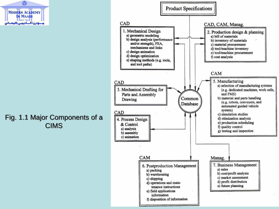
Fig. 1.1 Major Components of a

CIMS

BENEFITS OF CAD

The unique capabilities of CAD outlined above provide substantial benefits to

industrial users.

1. CAD can enhance the quality of engineering design with excellent graphical

representation of product geometries and production drawings.

2. It enables engineers to visually inspect the geometry of the product from

every conceivable viewing angle. The need to build prototypes of the

product, as required in many traditional design processes, has thus

diminished. Geometric definition of the product can be thoroughly studied

and modified by CAD.

3. Graphic simulation and animation of a CAD system can be used to inspect

the tolerance and interference of matching components of a product. They

can minimize errors in specifying such tolerances and interferences of

fittings.

4. Ever-improving and increasingly available computing power has further

extended the use of CAD for design problems involving hundreds of

variables. Many CAD systems can provide engineers with optimum solutions

for these complex problems.

5. CAD offers great flexibility and economy in the management of design data,

which include all pertinent design information and product geometries. It

provides engineers with the means to easily modify existing design files and

production drawings and saves storage space.

6. Many CAD systems can be interfaced directly to a CAM system that uses

intelligent machines to carry out production without human intervention. Such

an interface can reduce human error and result in a highly efficient, highly

accurate production system.

CHARACTERISTICS OF CAD

• There are many obvious differences in the ways in which CAD and the

traditional method are used in engineering design. It is useful for engineers

to recognize the unique characteristics of CAD in order to use this tool

effectively.

• The two principal characteristics of CAD are its dependence on software

programs and its strong basis on computer algorithms. Following is a brief

description of each.

CAD and Software:

There are generally two types of software programs: system software and

application software.

a) System software

used for the internal data management and operations of the components

is normally supplied by the hardware manufacturer.

b) Application software

must either be purchased from a commercial outlet or be developed in

house. Design engineers are expected to be users, but not developers, of

software. In most cases, they can operate the CAD system, which involves

both hardware and software, as a "black box". They do not have access to

the contents of the software as they would otherwise have with the

handbooks, the design codes, and the mathematical formulas, as in the

case of traditional design. However, it is essential that they be

knowledgeable about the principles of the application software used for the

job so that they can prepare the input and interpret the output correctly in

an engineering sense.

CAD and Computer Algorithms

All computations performed by a computer are based on the discrete sets

concept. In other words, all physical variables and functions, including "smooth"

curves, can only be handled in discrete or incremental piecewise linear forms.

Algorithms with iterative procedures for numerical approximations are thus

standard practice. The same concept applies to the graphics algorithms. For

example, a circle appearing on a monitor screen may well be a polygon

composed of many minute straight-line segments. Code developers require

adequate knowledge in adopting the most effective algorithm for the problem at

hand, and users must have sound engineering common sense in selecting the

right sizes of increments in both time and space domains.

Overall, it appears that the most fundamental difference between traditional

design and the CAD process lies not in the design methodology, but in the

implementation of the design method. Computerization of the design process

can produce quick, accurate design analyses and impressive, easily modifiable

interactive graphics displays, but the fundamental design principles remain

intact. It is inconceivable that an engineering designer can command a CAD

system effectively and produce good designs without adequate knowledge of

the traditional engineering disciplines.

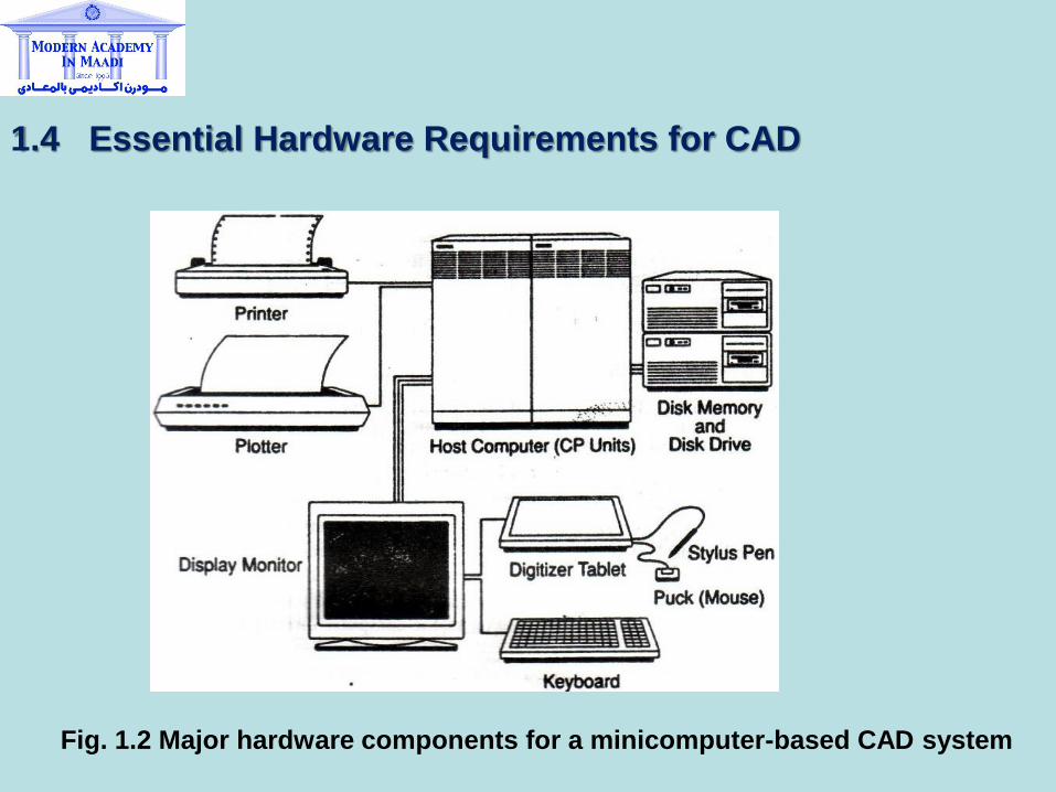
1.4 Essential Hardware Requirements for CAD

Fig. 1.2 Major hardware components for a minicomputer-based CAD system

1.5 Interactive Computer Graphics

The team interactive computer graphics refers to the real-time or

"instantaneous communication with the computer by the designer or operator.

This form of communication offers the operator much more freedom over the

traditional input methods that use the card deck and the keyboard. An effective

interactive computer graphic system allows sketching, drawing to be both input

to, and output from the computer. A fully interactive graphics system has almost

instant feedback from the graphic input by the designer. Three general types of

interactive graphics descriptions are used in computer-aided design and

analysis:

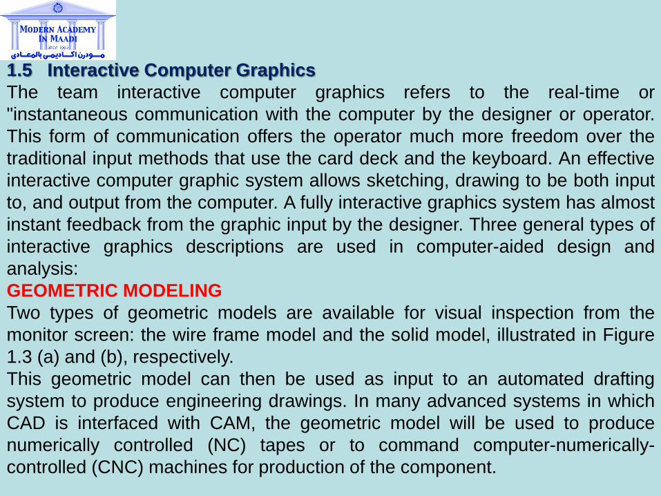
GEOMETRIC MODELING

Two types of geometric models are available for visual inspection from the

monitor screen: the wire frame model and the solid model, illustrated in Figure

1.3 (a) and (b), respectively.

This geometric model can then be used as input to an automated drafting

system to produce engineering drawings. In many advanced systems in which

CAD is interfaced with CAM, the geometric model will be used to produce

numerically controlled (NC) tapes or to command computer-numerically-

controlled (CNC) machines for production of the component.

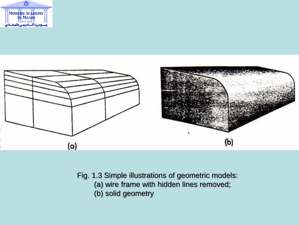
Fig. 1.3 Simple illustrations of geometric models:

(a) wire frame with hidden lines removed;

(b) solid geometry

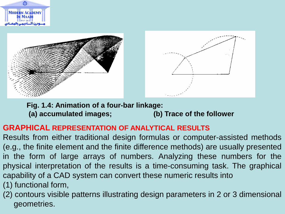
GRAPHICAL REPRESENTATION OF ANALYTICAL RESULTS

Results from either traditional design formulas or computer-assisted methods

(e.g., the finite element and the finite difference methods) are usually presented

in the form of large arrays of numbers. Analyzing these numbers for the

physical interpretation of the results is a time-consuming task. The graphical

capability of a CAD system can convert these numeric results into

(1) functional form,

(2) contours visible patterns illustrating design parameters in 2 or 3 dimensional

geometries.

Fig. 1.4: Animation of a four-bar linkage:

(a) accumulated images; (b) Trace of the follower

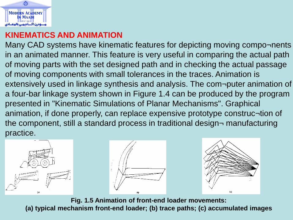
KINEMATICS AND ANIMATION

Many CAD systems have kinematic features for depicting moving compo¬nents

in an animated manner. This feature is very useful in comparing the actual path

of moving parts with the set designed path and in checking the actual passage

of moving components with small tolerances in the traces. Animation is

extensively used in linkage synthesis and analysis. The com¬puter animation of

a four-bar linkage system shown in Figure 1.4 can be produced by the program

presented in "Kinematic Simulations of Planar Mechanisms". Graphical

animation, if done properly, can replace expensive prototype construc¬tion of

the component, still a standard process in traditional design¬ manufacturing

practice.

Fig. 1.5 Animation of front-end loader movements:

(a) typical mechanism front-end loader; (b) trace paths; (c) accumulated images

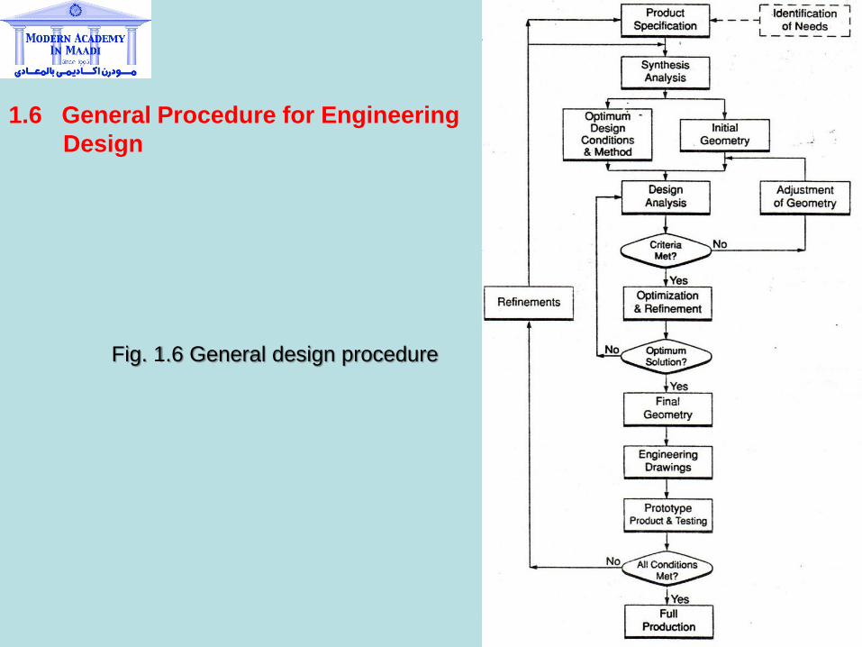
1.6 General Procedure for Engineering

Design

Fig. 1.6 General design procedure

1.8 Summary

The word CAD has become one of the most frequently mentioned technical

terms in recent years. Despite its popularity, the interpretation of its real

meaning as well as its relationship with traditional design is far from unanimous.

This chapter provides the reader with an overview of this subject and its

relationship with the computer-integrated manufacturing system.

Although CAD appears to be a new technology to many people, its real

essence, in the authors' view, does not deviate significantly from traditional

design philosophy and methodology. CAD gives designers much better and

more effective tools with which to produce better-quality design work.

Despite the close similarity between CAD and the traditional design method,

the reader should not underestimate the great value of the CAD in design

technology. No one can dispute the fact that CAD, even at its present state-of-

the-art, can provide designers with many unique capabilities, which would

never have been thought possible with the traditional method. With these

additional capabilities, designers can handle projects that involve a great many

more variables and constraints as well as complexities and varieties in terms of

product geometry and design conditions. It is a new challenge to the

engineering profession, and success in facing this challenge lies in how

effectively engineers can use this new tool.

High-level engineering analysis and interactive graphics are the two major

ingredients of most CAD systems: In addition to the obvious requirements for

the high quality of these two elements and the hardware facilities, the effective

use of CAD systems also depends on the user's appreciation and knowledge

of these elements. The remainder of the book will illustrate basic principles of

these elements.

CHAPTER 2

Review of Numerical Techniques for CAD 2.1 Introduction Digital computers play a very important role in modern engineering design and analysis. Engineers now use this effective tool to solve complex problems that would never have been thought possible only decades ago. However, the power of computers at the present level of technology lies in their incredible speed and memory capacity, but not in any intelligence or independent judgment. These machines essentially are capable of performing only simple arithmetical functions. Numerical techniques, sometimes referred to as numerical analyses; are used in wide spectrum of the physical sciences, and numerous books and monographs are specially devoted to this subject. Because it is not possible to cover in this chapter all the topics involved in numerical analysis, the reader is referred to the above references for wide-ranging, rigorous treatment of such topics. In this chapter, we will present the principles of some key topics that are particularly relevant to the applications in computer-aided design. Most of the topics reviewed herein will be used in other parts of the book.

2.2 Matrices and Determinants See MATLAB course

2.3 Solution of Simultaneous Linear Equations a) See MATLAB course

b) Gaussian Elimination Method

c) Cholesky Lu Decomposition 2.4 Eigenvalue Problems One type of design analysis that engineers often encounter is eigenvalue problems. The solution of eigenvalue problems also requires the solution of simultaneous algebraic equations. Unique solutions to these equations are possible only if the value of a parameter involved in these equations is known. This parameter is referred to as an eigenvalue. The solution to the equations corresponding to each eigenvalue is called the eigenvector of that eigenvalue. Eigenvalues are associated with the natural frequencies of a structure in a modal analysis, and eigenvectors characterize the shapes of corresponding modes of vibration. Eigenvalues also determine the critical loads for stability analyses of structures, in which the eigenvalues are used to compute the critical loads that cause the instability of the structure.

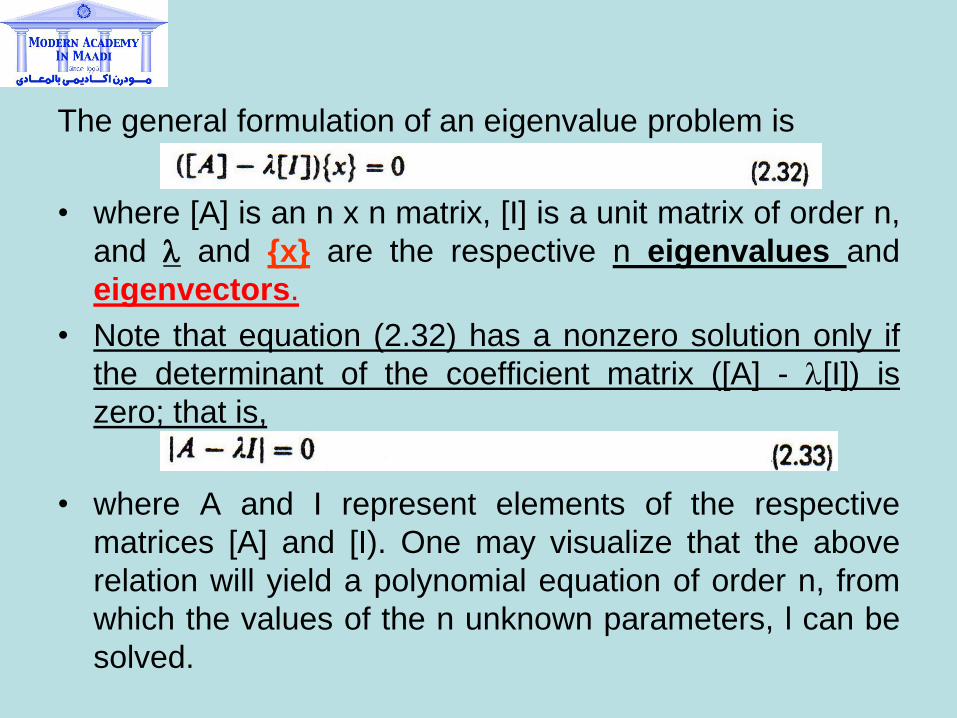
The general formulation of an eigenvalue problem is

• where [A] is an n x n matrix, [I] is a unit matrix of order n,

and l and {x} are the respective n eigenvalues and

eigenvectors.

• Note that equation (2.32) has a nonzero solution only if

the determinant of the coefficient matrix ([A] - l[I]) is

zero; that is,

• where A and I represent elements of the respective

matrices [A] and [I). One may visualize that the above

relation will yield a polynomial equation of order n, from

which the values of the n unknown parameters, l can be

solved.

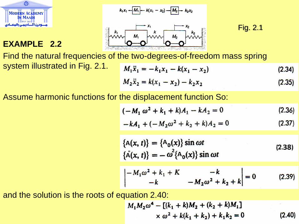
EXAMPLE 2.2

Find the natural frequencies of the two-degrees-of-freedom mass spring

system illustrated in Fig. 2.1.

Assume harmonic functions for the displacement function So:

and the solution is the roots of equation 2.40:

Fig. 2.1

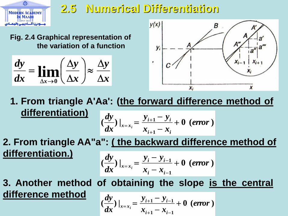
2.5 Numerical Differentiation

Fig. 2.4 Graphical representation of

the variation of a function

x

y

x

y

dx

dy

x

lim

0

1. From triangle A'Aa': (the forward difference method of

differentiation) )( 0|)(

1

1 errorxx

yy

dx

dy

ii

ii

xx i

2. From triangle AA"a": ( the backward difference method of

differentiation.)

)( 0|)(1

1 errorxx

yy

dx

dy

ii

ii

xx i

3. Another method of obtaining the slope is the central

difference method )( 0|)(

11

11 errorxx

yy

dx

dy

ii

ii

xx i

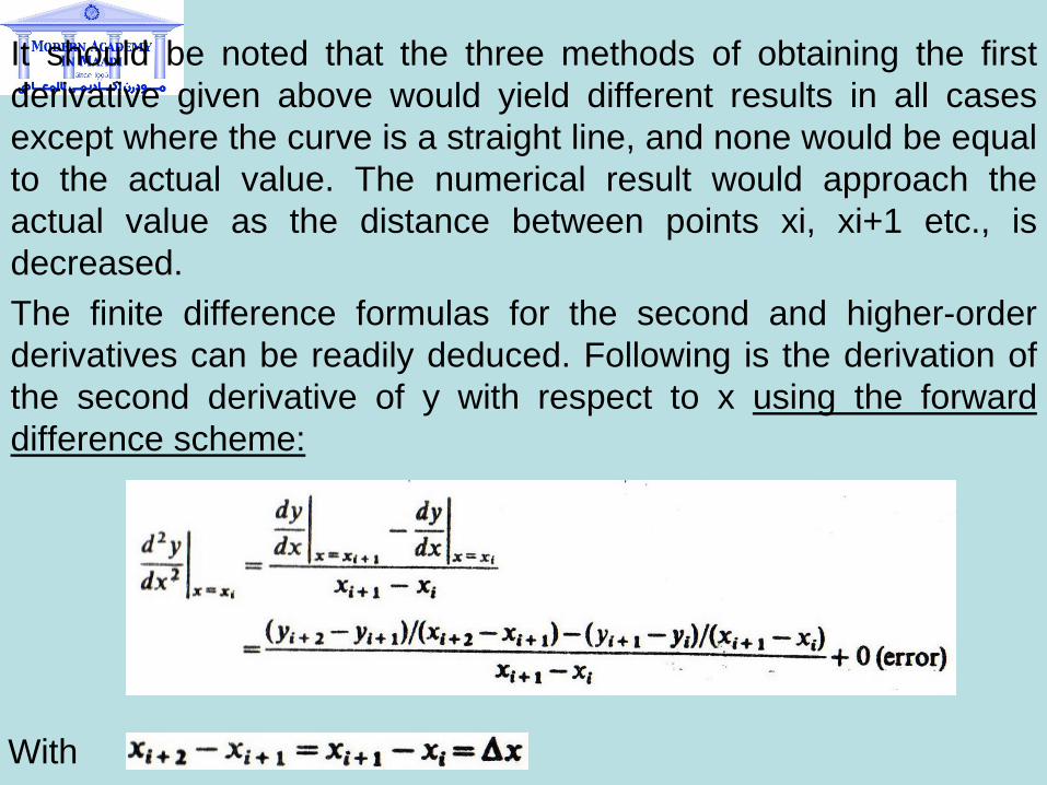
It should be noted that the three methods of obtaining the first

derivative given above would yield different results in all cases

except where the curve is a straight line, and none would be equal

to the actual value. The numerical result would approach the

actual value as the distance between points xi, xi+1 etc., is

decreased.

The finite difference formulas for the second and higher-order

derivatives can be readily deduced. Following is the derivation of

the second derivative of y with respect to x using the forward

difference scheme:

With

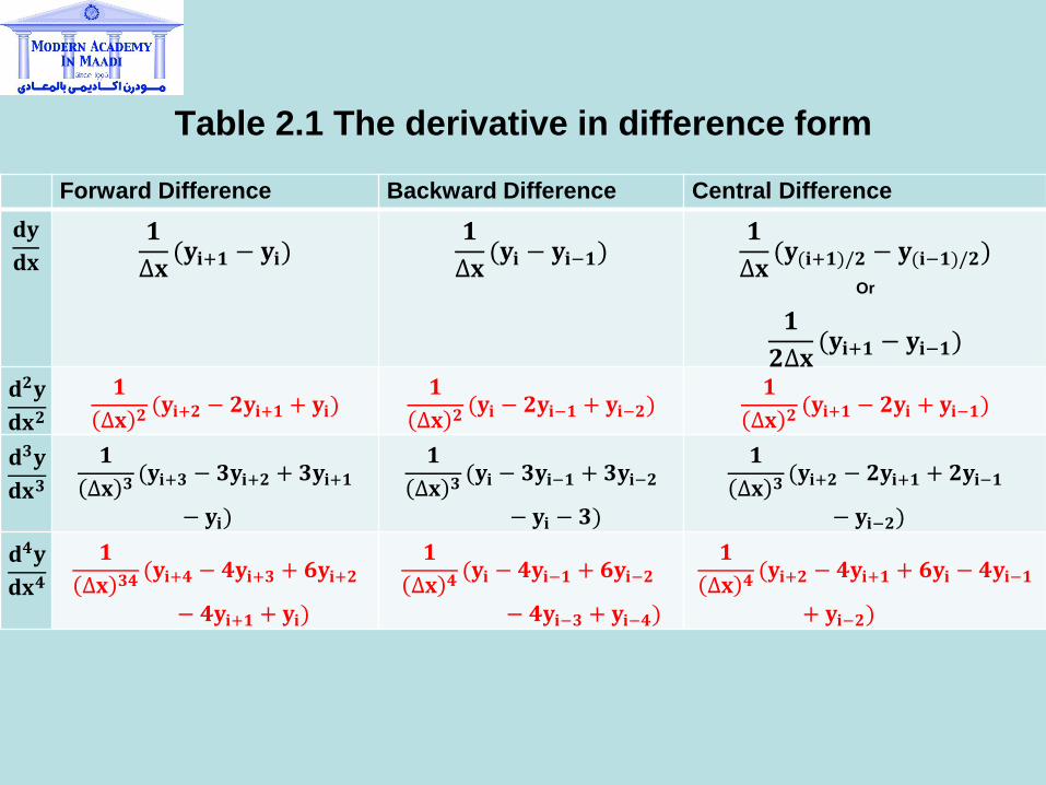
Table 2.1 The derivative in difference form

Forward Difference Backward Difference Central Difference

𝐝𝐲

𝐝𝐱

𝟏

∆𝐱(𝐲𝐢+𝟏 − 𝐲𝐢)

𝟏

∆𝐱(𝐲𝐢 − 𝐲𝐢−𝟏)

𝟏

∆𝐱(𝐲(𝐢+𝟏)/𝟐 − 𝐲(𝐢−𝟏)/𝟐)

Or

𝟏

𝟐∆𝐱(𝐲𝐢+𝟏 − 𝐲𝐢−𝟏)

𝐝𝟐𝐲

𝐝𝐱𝟐

𝟏

∆𝐱 𝟐(𝐲𝐢+𝟐 − 𝟐𝐲𝐢+𝟏 + 𝐲𝐢)

𝟏

∆𝐱 𝟐(𝐲𝐢 − 𝟐𝐲𝐢−𝟏 + 𝐲𝐢−𝟐)

𝟏

∆𝐱 𝟐(𝐲𝐢+𝟏 − 𝟐𝐲𝐢 + 𝐲𝐢−𝟏)

𝐝𝟑𝐲

𝐝𝐱𝟑

𝟏

∆𝐱 𝟑(𝐲𝐢+𝟑 − 𝟑𝐲𝐢+𝟐 + 𝟑𝐲𝐢+𝟏

− 𝐲𝐢)

𝟏

∆𝐱 𝟑(𝐲𝐢 − 𝟑𝐲𝐢−𝟏 + 𝟑𝐲𝐢−𝟐

− 𝐲𝐢 − 𝟑)

𝟏

∆𝐱 𝟑(𝐲𝐢+𝟐 − 𝟐𝐲𝐢+𝟏 + 𝟐𝐲𝐢−𝟏

− 𝐲𝐢−𝟐)

𝐝𝟒𝐲

𝐝𝐱𝟒

𝟏

∆𝐱 𝟑𝟒(𝐲𝐢+𝟒 − 𝟒𝐲𝐢+𝟑 + 𝟔𝐲𝐢+𝟐

− 𝟒𝐲𝐢+𝟏 + 𝐲𝐢)

𝟏

∆𝐱 𝟒(𝐲𝐢 − 𝟒𝐲𝐢−𝟏 + 𝟔𝐲𝐢−𝟐

− 𝟒𝐲𝐢−𝟑 + 𝐲𝐢−𝟒)

𝟏

∆𝐱 𝟒(𝐲𝐢+𝟐 − 𝟒𝐲𝐢+𝟏 + 𝟔𝐲𝐢 − 𝟒𝐲𝐢−𝟏

+ 𝐲𝐢−𝟐)

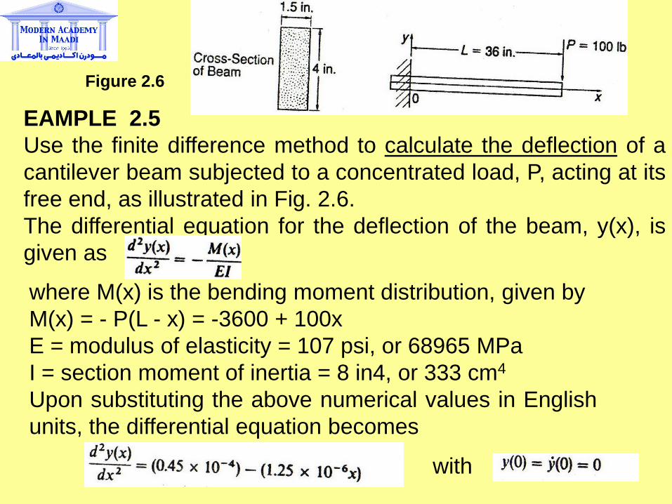
EAMPLE 2.5

Use the finite difference method to calculate the deflection of a

cantilever beam subjected to a concentrated load, P, acting at its

free end, as illustrated in Fig. 2.6.

The differential equation for the deflection of the beam, y(x), is

given as

Figure 2.6

where M(x) is the bending moment distribution, given by

M(x) = - P(L - x) = -3600 + 100x

E = modulus of elasticity = 107 psi, or 68965 MPa

I = section moment of inertia = 8 in4, or 333 cm4

Upon substituting the above numerical values in English

units, the differential equation becomes

with

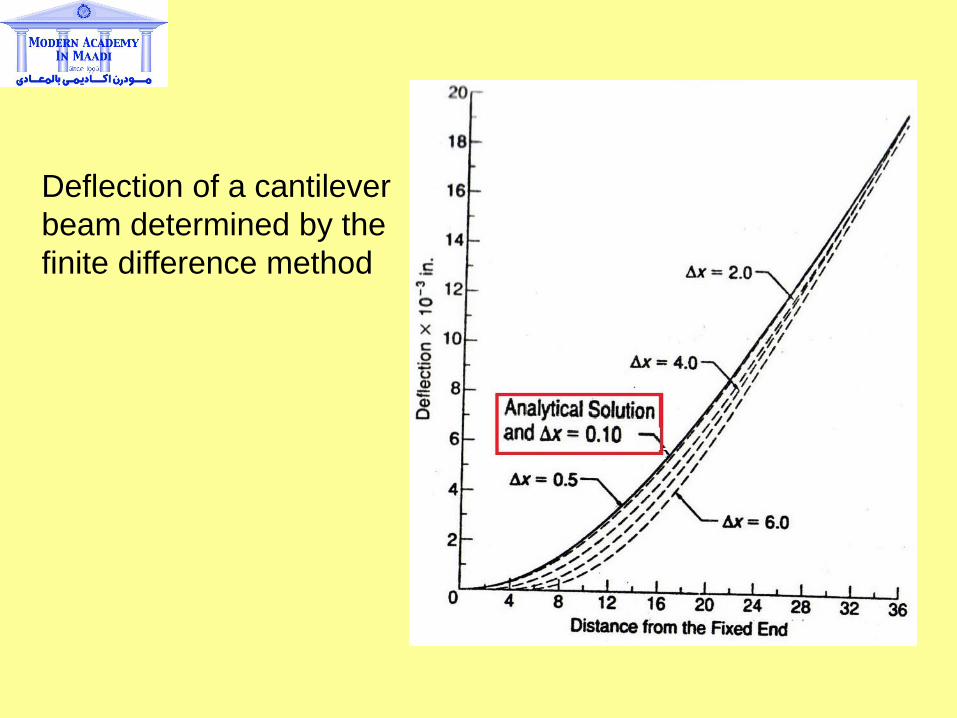
Deflection of a cantilever

beam determined by the

finite difference method

2.6 Numerical Integration

Numerical integration of o

function y(x) between two

specified intervals

a) TRAPEZOIDAL RULE

The accuracy of the above expression depends on how close

the curve AB in previous Figure can be approximated by the

series of straight-line segments.

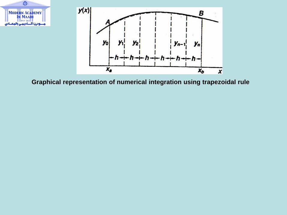
Graphical representation of numerical integration using trapezoidal rule

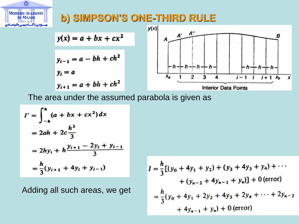
b) SIMPSON'S ONE-THIRD RULE

The area under the assumed parabola is given as

Adding all such areas, we get

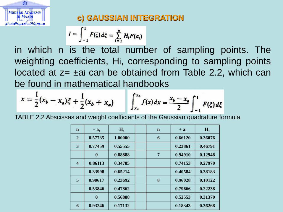
c) GAUSSIAN INTEGRATION

in which n is the total number of sampling points. The

weighting coefficients, Hi, corresponding to sampling points

located at z= ±ai can be obtained from Table 2.2, which can

be found in mathematical handbooks

TABLE 2.2 Abscissas and weight coefficients of the Gaussian quadrature formula

n + a1 H1 n + a1 H1

2 0.57735 1.00000 6 0.66120 0.36076

3 0.77459 0.55555 0.23861 0.46791

0 0.88888 7 0.94910 0.12948

4 0.86113 0.34785 0.74153 0.27970

0.33998 0.65214 0.40584 0.38183

5 0.90617 0.23692 8 0.96028 0.10122

0.53846 0.47862 0.79666 0.22238

0 0.56888 0.52553 0.31370

6 0.93246 0.17132 0.18343 0.36268

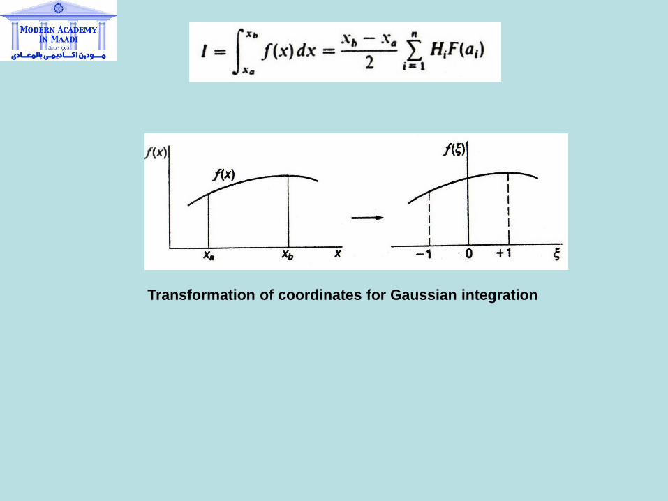
Transformation of coordinates for Gaussian integration

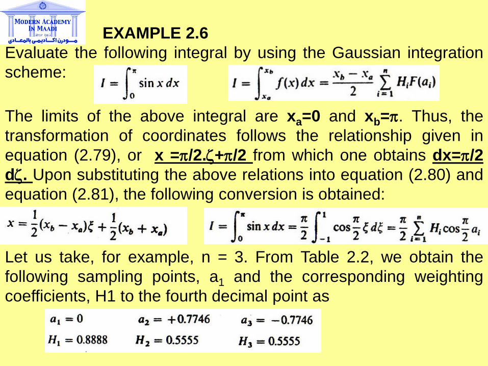
EXAMPLE 2.6

Evaluate the following integral by using the Gaussian integration

scheme:

The limits of the above integral are xa=0 and xb=p. Thus, the

transformation of coordinates follows the relationship given in

equation (2.79), or x =p/2.z+p/2 from which one obtains dx=p/2

dz. Upon substituting the above relations into equation (2.80) and

equation (2.81), the following conversion is obtained:

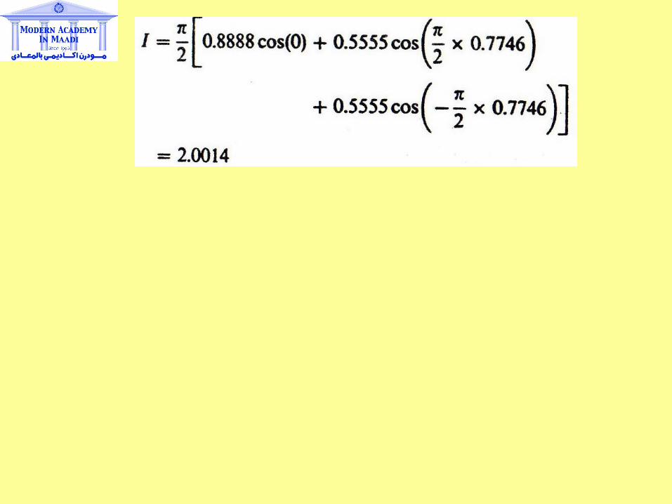
Let us take, for example, n = 3. From Table 2.2, we obtain the

following sampling points, a1 and the corresponding weighting

coefficients, H1 to the fourth decimal point as

2.7 Summary Complicated mathematical functions and equations are often used

in performing design analysis and producing geometric models in

CAD. Numerical techniques must be used to convert these

functions and equations into simple arithmetical operations that

can be handled by digital computers. The purpose of this chapter

is to provide the reader with a brief review of some key elements

that are relevant to CAD and analysis.

Numerical techniques are necessary to convert complicated

mathematical manipulations into simple arithmetical operations

that are manageable by digital computers. Readers, however,

must be aware of the inherent errors in such practice. Recognition

of these errors and intelligent use of various numerical analysis

schemes are critical to the accuracy of the results.

CHAPTER 3

Principles of Computer Graphics 2.1 Introduction In this chapter, curve, surface and solid modeling will be described in detail, with the aim of giving the reader an understanding of the nature of the modeling techniques and of their theoretical basis.

3.2 Mathematical formulations for Graphics a) LINES

Straight lines form the basis for the display of all types of shapes, whether two-dimensional or three-dimensional, in computer graphics. A circle, for example, may be drawn by joining a large number of small line segments. In a similar fashion, a sphere can be drawn by joining a number of triangular shapes, which in turn may be created by joining three straight lines.

In DDA (Digital differential analyzer), the equation of a line is expressed as a pair of parametric equations:

x = x1 + (x2 – x1)*s (3.1)

y = y1 + (y2 – y1)*s (3.2)

where the parameter s varies from 0 to 1. If s is incremented by, say, 0.1, then the DDA will generate 9 points in between the two ends of the line.

Once the addresses of all the pixels are determined, these are stored in a frame buffer. The display driver reads the array of addresses and illuminates the corresponding pixels. In order for a line to look continuous, it is necessary to increment the parameter s in a manner consistent with the resolution of the display device. If too large an increment is selected, the line may appear to be discontinuous. If too small an increment is selected, a large number of pixels near each other are illuminated, and the line appears thicker and brighter, but the drawing process becomes slower.

b) CIRCLES

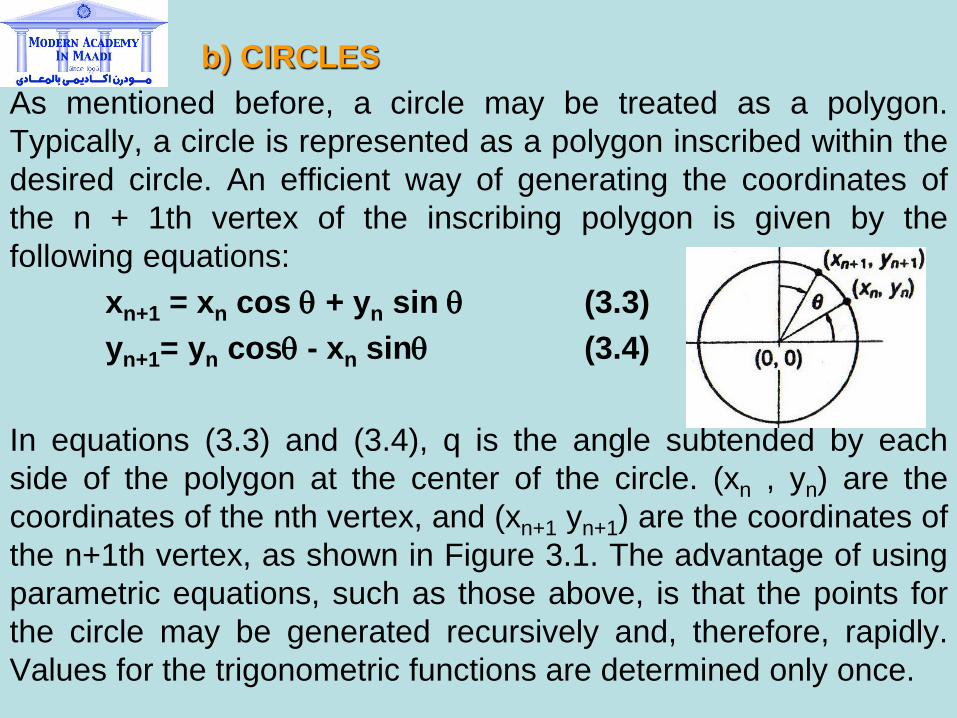
As mentioned before, a circle may be treated as a polygon.

Typically, a circle is represented as a polygon inscribed within the

desired circle. An efficient way of generating the coordinates of

the n + 1th vertex of the inscribing polygon is given by the

following equations:

xn+1 = xn cos q + yn sin q (3.3)

yn+1= yn cosq - xn sinq (3.4)

In equations (3.3) and (3.4), q is the angle subtended by each

side of the polygon at the center of the circle. (xn , yn) are the

coordinates of the nth vertex, and (xn+1 yn+1) are the coordinates of

the n+1th vertex, as shown in Figure 3.1. The advantage of using

parametric equations, such as those above, is that the points for

the circle may be generated recursively and, therefore, rapidly.

Values for the trigonometric functions are determined only once.

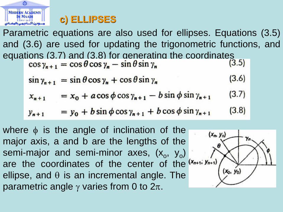
c) ELLIPSES

Parametric equations are also used for ellipses. Equations (3.5)

and (3.6) are used for updating the trigonometric functions, and

equations (3.7) and (3.8) for generating the coordinates

where f is the angle of inclination of the

major axis, a and b are the lengths of the

semi-major and semi-minor axes, (xo, yo)

are the coordinates of the center of the

ellipse, and q is an incremental angle. The

parametric angle g varies from 0 to 2p.

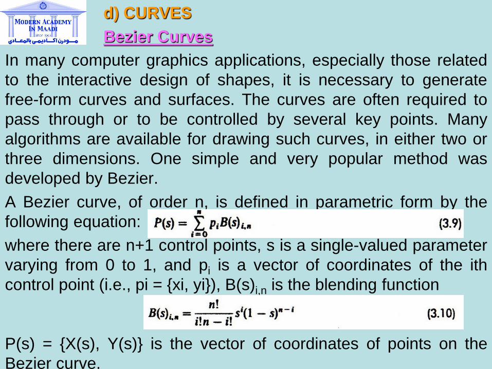
d) CURVES

Bezier Curves

In many computer graphics applications, especially those related

to the interactive design of shapes, it is necessary to generate

free-form curves and surfaces. The curves are often required to

pass through or to be controlled by several key points. Many

algorithms are available for drawing such curves, in either two or

three dimensions. One simple and very popular method was

developed by Bezier.

A Bezier curve, of order n, is defined in parametric form by the

following equation:

where there are n+1 control points, s is a single-valued parameter

varying from 0 to 1, and pi is a vector of coordinates of the ith

control point (i.e., pi = {xi, yi}), B(s)i,n is the blending function

P(s) = {X(s), Y(s)} is the vector of coordinates of points on the

Bezier curve.

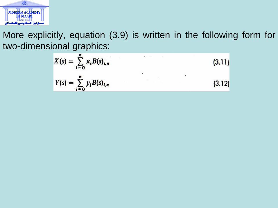
More explicitly, equation (3.9) is written in the following form for

two-dimensional graphics:

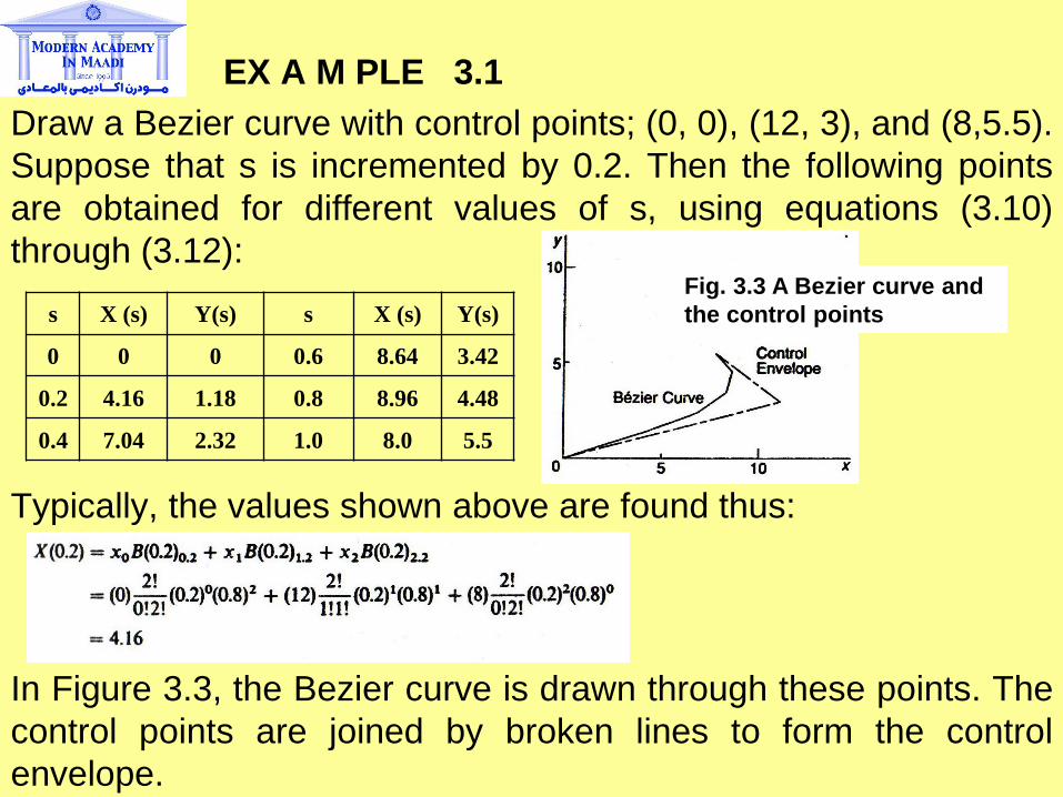
EX A M PLE 3.1

Draw a Bezier curve with control points; (0, 0), (12, 3), and (8,5.5).

Suppose that s is incremented by 0.2. Then the following points

are obtained for different values of s, using equations (3.10)

through (3.12):

Typically, the values shown above are found thus:

In Figure 3.3, the Bezier curve is drawn through these points. The

control points are joined by broken lines to form the control

envelope.

s X (s) Y(s) s X (s) Y(s)

0 0 0 0.6 8.64 3.42

0.2 4.16 1.18 0.8 8.96 4.48

0.4 7.04 2.32 1.0 8.0 5.5

Fig. 3.3 A Bezier curve and

the control points

As is seen from equations (3.11) and (3.12), the blending functions act as links between the coordinates of the control points and the points on the Bezier curve. If there are n + 1 control points, there will be exactly the same number of separate blending functions for each value of s. At s=0 (i.e., at the 0th control point), the blending function B0,1=1 and all other blending functions are zero. As a result, the first point on the Bezier curve coincides with the 0th control point. Similarly, the last point on the B6zier curve coincides with the (n+1)th. control point. In general, a Bezier curve does not pass through any other control points, as shown in Example 3.1.

Although simple to use and apply, the Bezier method has certain disadvantages. It is generally difficult to predict the shape of the curve since it does not pass through most of the control points. Thus, problems arise in modeling complex profiles. Usually, in such situations, multiple Bezier curves are required -joined end to end- to produce the desired shape.

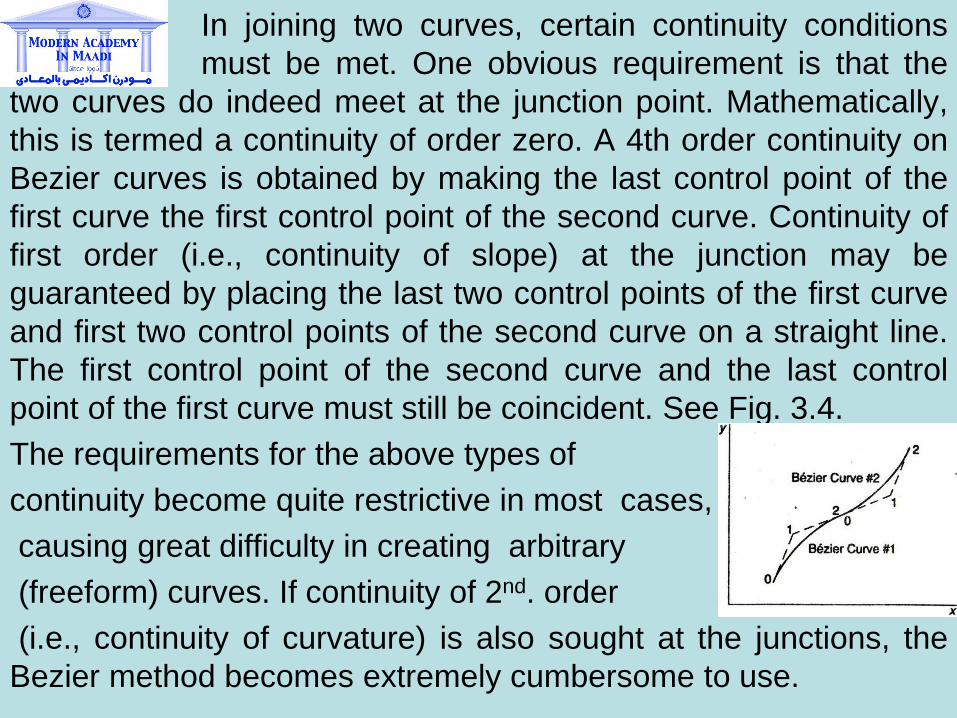
In joining two curves, certain continuity conditions

must be met. One obvious requirement is that the

two curves do indeed meet at the junction point. Mathematically,

this is termed a continuity of order zero. A 4th order continuity on

Bezier curves is obtained by making the last control point of the

first curve the first control point of the second curve. Continuity of

first order (i.e., continuity of slope) at the junction may be

guaranteed by placing the last two control points of the first curve

and first two control points of the second curve on a straight line.

The first control point of the second curve and the last control

point of the first curve must still be coincident. See Fig. 3.4.

The requirements for the above types of

continuity become quite restrictive in most cases,

causing great difficulty in creating arbitrary

(freeform) curves. If continuity of 2nd. order

(i.e., continuity of curvature) is also sought at the junctions, the

Bezier method becomes extremely cumbersome to use.

Piecewise Polynomial Functions

A more flexible method for producing arbitrary curves uses piecewise polynomial (pp) functions. A convenient method of generating pp functions is that of polynomial B-splines. Another form of B-spline is the beta spline [3], in which bias and tension parameters are used to produce additional flexibility. Rational B-spline curves, in which the scale factors (Section 3.6) in the homogeneous coordinate system are different from 1, are also powerful in generating free-form curves, conic sections, circles, etc. Some discussion on NONUNIFORM RATIONAL B-SPLINES, known as NURBS, follows the discussion on the polynomial B-splines. It is, however, advised that students familiarize themselves with the concept of the homogeneous coordinate system before reading about NURBS.

Polynomial B-splines

A piecewise polynomial function consists of a number of different polynomial functions joined together to form a single curve. The points at which segments of the polynomial curves are joined are known as knots or joints. There are several types of piecewise polynomials possible (e.g., the piecewise cubic polynomial, such as that used in Section 3.3 for curve fitting). Piecewise cubic Hermite polynomials (splines) are also used for curve fitting.

A polynomial spline P(s) of order k (degree k-1) is a pp function comprised of polynomial segments of degree less than k. Generally, it is assumed that the spline has continuity of order k-1 at all interior knots (i.e., at all knots away from the ends of the curve). It is possible nonetheless, and often advantageous, to maintain a higher or lower order of continuity at one or all of the interior knots.

A spline P(s) may be represented as a linear combination of basis or B-splines in the following manner:

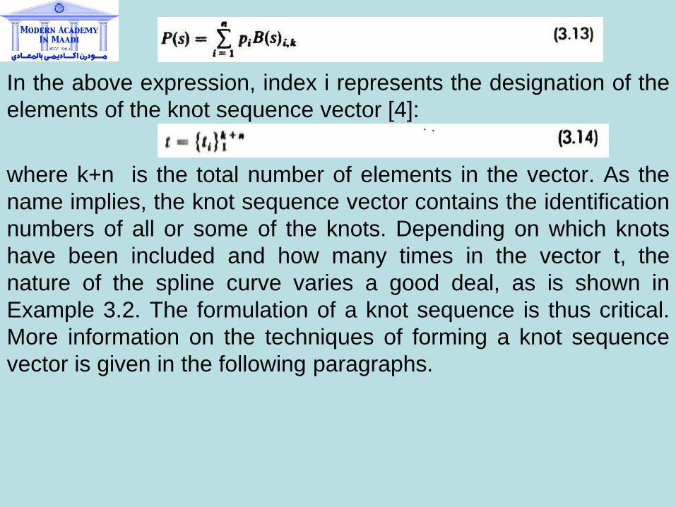
In the above expression, index i represents the designation of the

elements of the knot sequence vector [4]:

where k+n is the total number of elements in the vector. As the

name implies, the knot sequence vector contains the identification

numbers of all or some of the knots. Depending on which knots

have been included and how many times in the vector t, the

nature of the spline curve varies a good deal, as is shown in

Example 3.2. The formulation of a knot sequence is thus critical.

More information on the techniques of forming a knot sequence

vector is given in the following paragraphs.

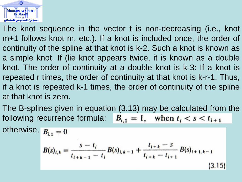
The knot sequence in the vector t is non-decreasing (i.e., knot

m+1 follows knot m, etc.). If a knot is included once, the order of

continuity of the spline at that knot is k-2. Such a knot is known as

a simple knot. If (lie knot appears twice, it is known as a double

knot. The order of continuity at a double knot is k-3: If a knot is

repeated r times, the order of continuity at that knot is k-r-1. Thus,

if a knot is repeated k-1 times, the order of continuity of the spline

at that knot is zero.

The B-splines given in equation (3.13) may be calculated from the

following recurrence formula:

otherwise,

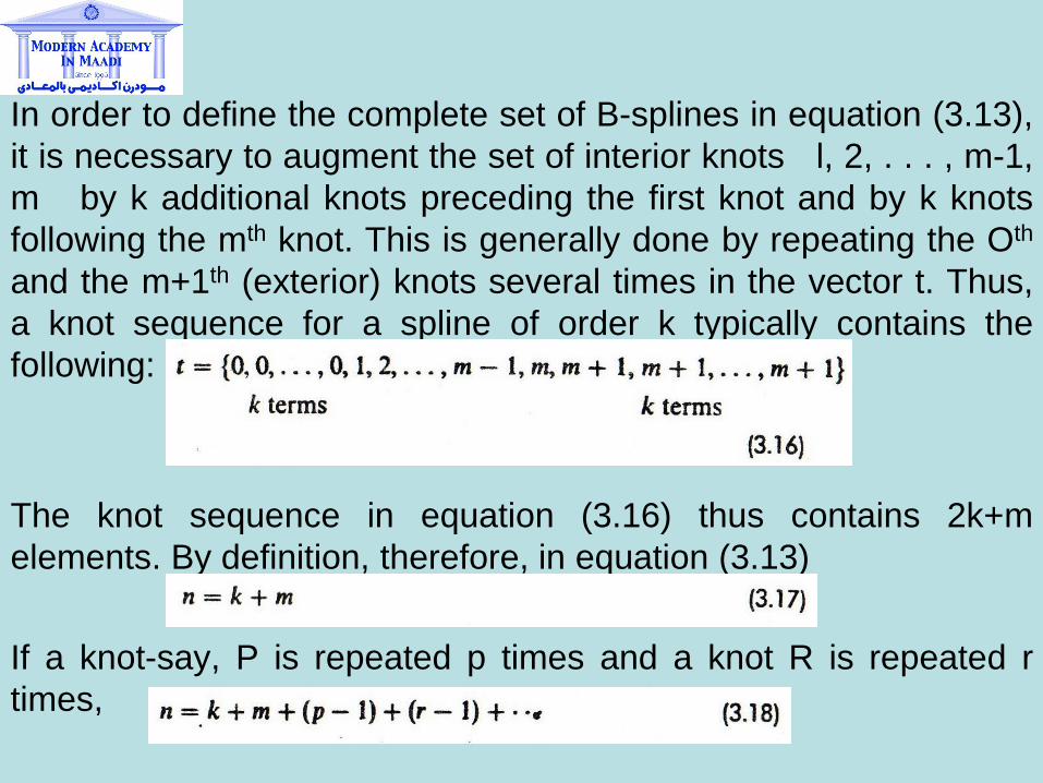
In order to define the complete set of B-splines in equation (3.13),

it is necessary to augment the set of interior knots l, 2, . . . , m-1,

m by k additional knots preceding the first knot and by k knots

following the mth knot. This is generally done by repeating the Oth

and the m+1th (exterior) knots several times in the vector t. Thus,

a knot sequence for a spline of order k typically contains the

following:

The knot sequence in equation (3.16) thus contains 2k+m

elements. By definition, therefore, in equation (3.13)

If a knot-say, P is repeated p times and a knot R is repeated r

times,

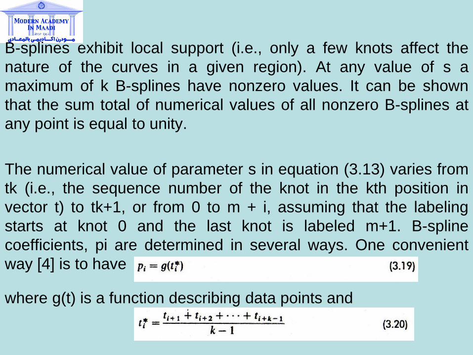
B-splines exhibit local support (i.e., only a few knots affect the

nature of the curves in a given region). At any value of s a

maximum of k B-splines have nonzero values. It can be shown

that the sum total of numerical values of all nonzero B-splines at

any point is equal to unity.

The numerical value of parameter s in equation (3.13) varies from

tk (i.e., the sequence number of the knot in the kth position in

vector t) to tk+1, or from 0 to m + i, assuming that the labeling

starts at knot 0 and the last knot is labeled m+1. B-spline

coefficients, pi are determined in several ways. One convenient

way [4] is to have

where g(t) is a function describing data points and

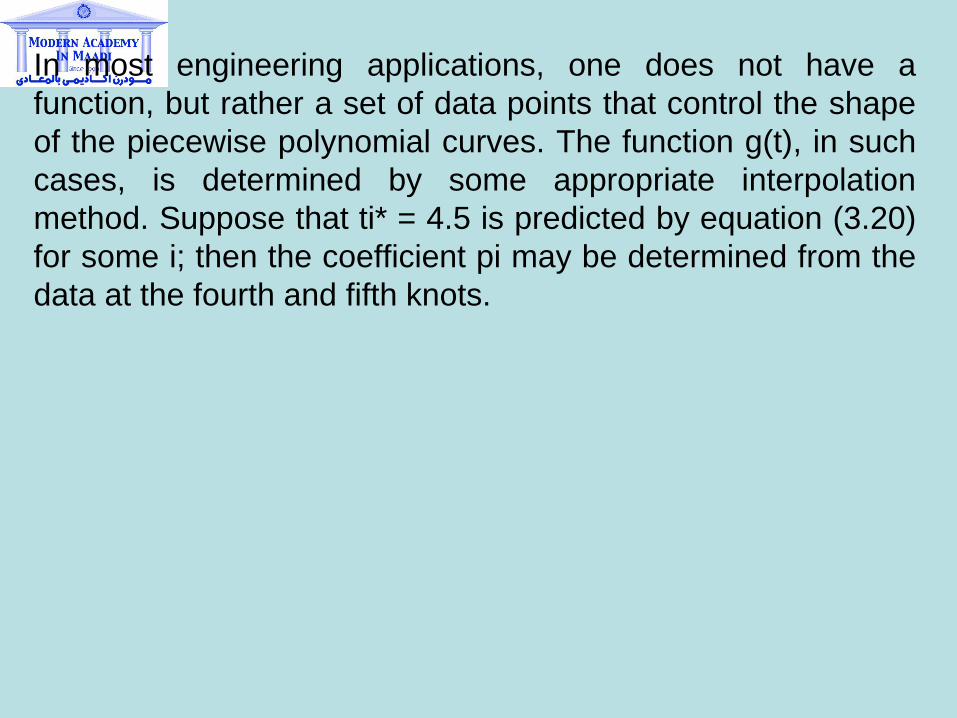
In most engineering applications, one does not have a

function, but rather a set of data points that control the shape

of the piecewise polynomial curves. The function g(t), in such

cases, is determined by some appropriate interpolation

method. Suppose that ti* = 4.5 is predicted by equation (3.20)

for some i; then the coefficient pi may be determined from the

data at the fourth and fifth knots.

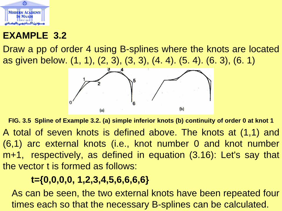
EXAMPLE 3.2

Draw a pp of order 4 using B-splines where the knots are located

as given below. (1, 1), (2, 3), (3, 3), (4. 4). (5. 4). (6. 3), (6. 1)

FIG. 3.5 Spline of Example 3.2. (a) simple inferior knots (b) continuity of order 0 at knot 1

A total of seven knots is defined above. The knots at (1,1) and

(6,1) arc external knots (i.e., knot number 0 and knot number

m+1, respectively, as defined in equation (3.16): Let's say that

the vector t is formed as follows:

t={0,0,0,0, 1,2,3,4,5,6,6,6,6}

As can be seen, the two external knots have been repeated four

times each so that the necessary B-splines can be calculated.

The internal knots occur only once, which means that the order of

continuity of thc pp is everywhere 2. The resulting 4th order curve

is shown in Figure 3.5(a).

Suppose that the vector t is reformulated as shown below.

r={0,0,0,0,1,1,1,2,3,4,5,6,6,6,6}

As explained before, with the above knot sequence vector,

continuity of the pp curve produced at knot 1 will be of order 0.

That fact is obvious from Figure 3.5(b).

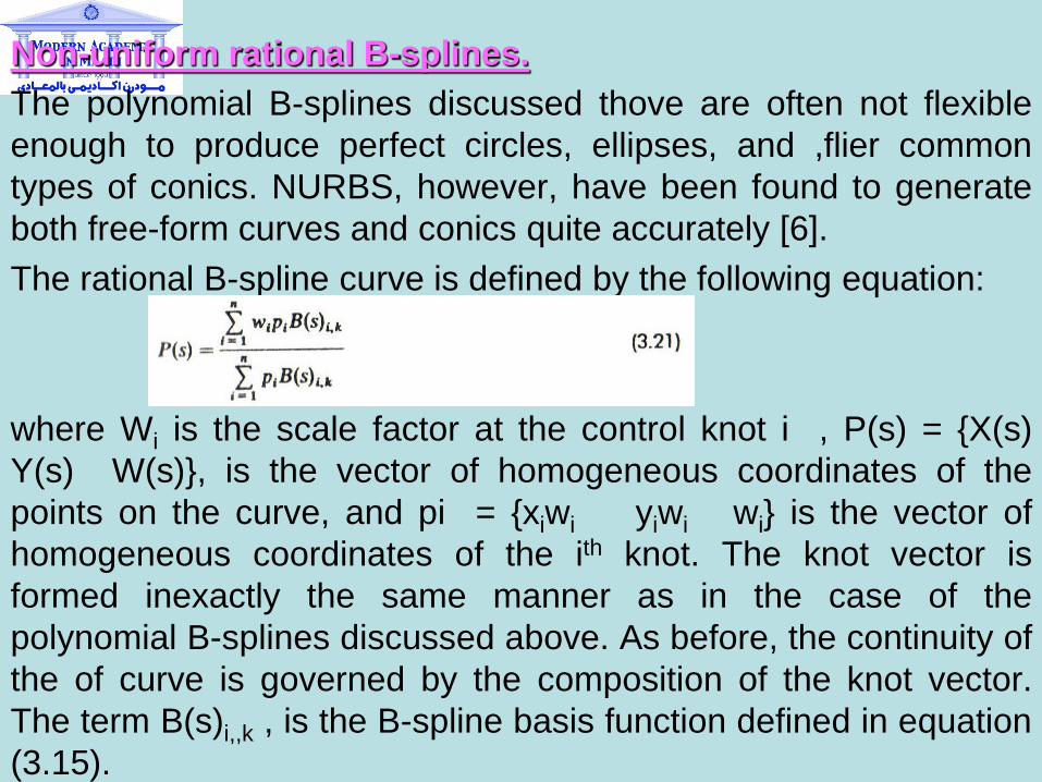
Non-uniform rational B-splines.

The polynomial B-splines discussed thove are often not flexible

enough to produce perfect circles, ellipses, and ,flier common

types of conics. NURBS, however, have been found to generate

both free-form curves and conics quite accurately [6].

The rational B-spline curve is defined by the following equation:

where Wi is the scale factor at the control knot i , P(s) = {X(s)

Y(s) W(s)}, is the vector of homogeneous coordinates of the

points on the curve, and pi = {xiwi yiwi wi} is the vector of

homogeneous coordinates of the ith knot. The knot vector is

formed inexactly the same manner as in the case of the

polynomial B-splines discussed above. As before, the continuity of

the of curve is governed by the composition of the knot vector.

The term B(s)i,,k , is the B-spline basis function defined in equation

(3.15).

3.3 Basic Curve-Fitting Techniques In many engineering applications, physical quantities are specified at a few discrete points, but not in the entire domain. The reader will find many such examples in practice. For instance, the data on strains in a structure are available at only a few selected points as measured by strain gauges. Interpolation or extrapolation procedures are used to determine values (such as strains in the example mentioned above) at points other than those specified or measured at the discrete points. Curve fitting is one of the techniques that can be used to achieve this purpose.

The geometry of a solid can be described by the topography of its surfaces, which consist of an infinite number of points. Each of these points can be uniquely described by a set of coordinates in the space. The description of the geometry of a solid surface and the storage and retrieval of this information thus, in theory, require the specification and storage. of an infinite number of sets of coordinates. This, of course, is not possible in reality. In such instances, curve-fitting techniques become extremely useful.

The essence of most curve-fitting techniques is to derive continuous functions that satisfy the values of certain variables specified at given points. The functions so derived yield approximate values of the variables at all other points. In a practical sense, it means that mathematical functions derived by curve-fitting techniques represent approximate variation of the physical quantity over a specified domain.

A number of curve-fitting techniques are described in the literatures. Here, we will introduce the three most basic techniques: (1) polynomial fitting, (2) polynomial regression with least square fit, and (3) spline interpolation. These techniques are not necessarily the most efficient ones for CAD applications. They are introduced primarily to illustrate the principles of curve-fitting by mathematical functions.

POLYNOMIAL CURVE-FITTING

The mathematical function used to represent the point values of a dependent variable Y, at discrete points Xi (i = 1, 2,.... , n + 1) may be assumed to be a polynomial function such as

Y(X) = A0 + A1 X + A2X2 + - - - + An Xn (3.22)

where A0, A1,..., An are constants to be determined by solving a set of simultaneous equations that are obtained by substituting pairs of specified values (X1, Y1) for the variables X and Y in equation (3.22).

The polynomial technique is simple to use. However, its accuracy depends on the number and the choice of data points. Equation (3.22) indicates that a quadratic function is the highest order of polynomial function that one may use for the case of three data points. Likewise, a cubic function would require tour data points. Thus, if N is the number of available data points, the order of the polynomial function n = N - 1.

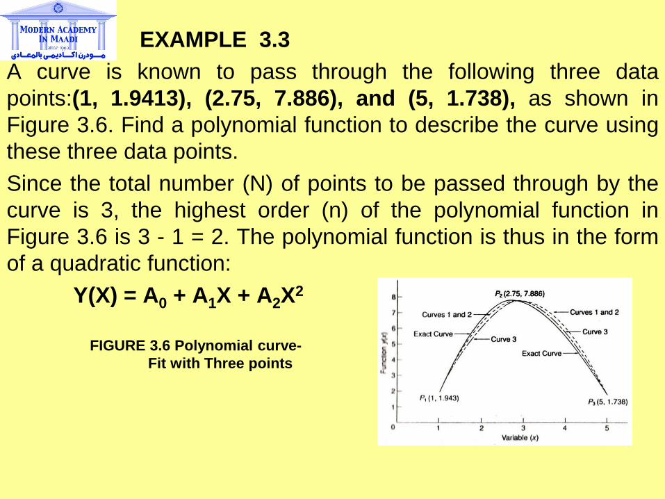
EXAMPLE 3.3

A curve is known to pass through the following three data

points:(1, 1.9413), (2.75, 7.886), and (5, 1.738), as shown in

Figure 3.6. Find a polynomial function to describe the curve using

these three data points.

Since the total number (N) of points to be passed through by the

curve is 3, the highest order (n) of the polynomial function in

Figure 3.6 is 3 - 1 = 2. The polynomial function is thus in the form

of a quadratic function:

Y(X) = A0 + A1X + A2X2

FIGURE 3.6 Polynomial curve-

Fit with Three points

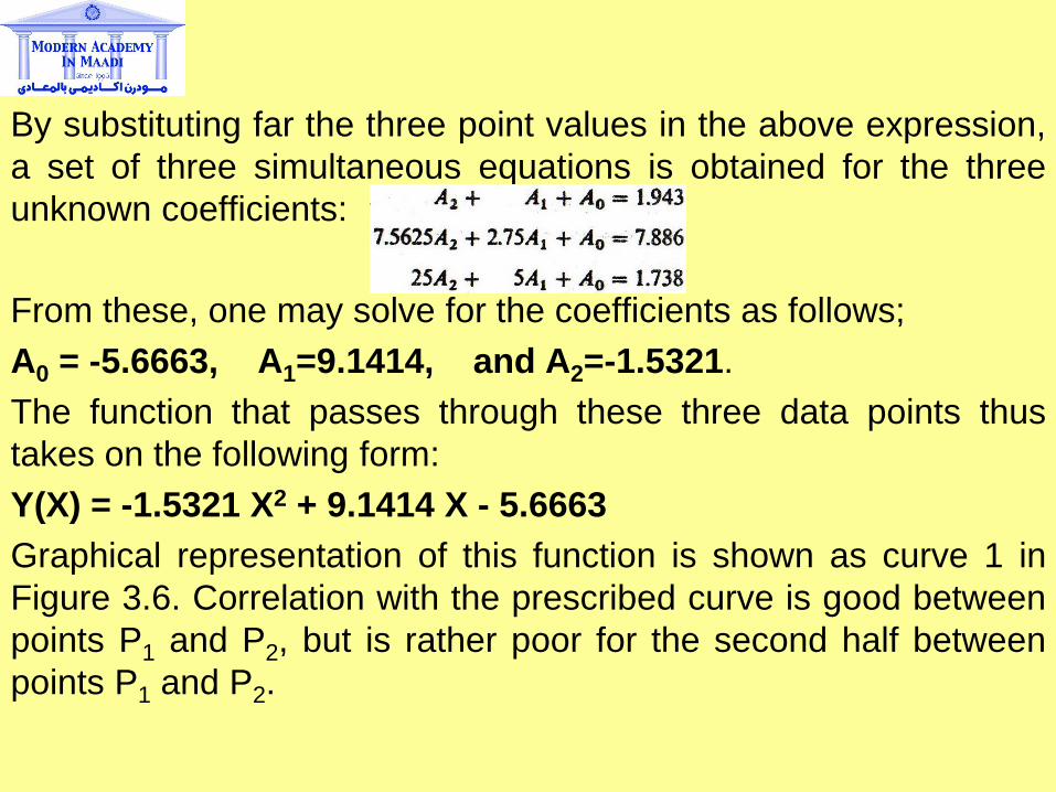
By substituting far the three point values in the above expression,

a set of three simultaneous equations is obtained for the three

unknown coefficients:

From these, one may solve for the coefficients as follows;

A0 = -5.6663, A1=9.1414, and A2=-1.5321.

The function that passes through these three data points thus

takes on the following form:

Y(X) = -1.5321 X2 + 9.1414 X - 5.6663

Graphical representation of this function is shown as curve 1 in

Figure 3.6. Correlation with the prescribed curve is good between

points P1 and P2, but is rather poor for the second half between

points P1 and P2.

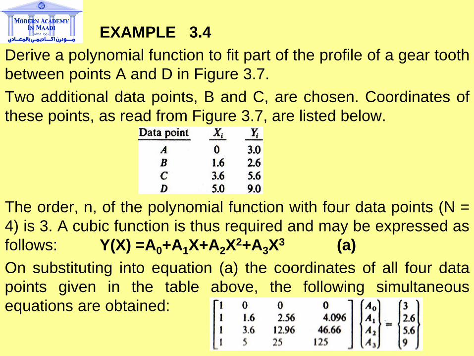
EXAMPLE 3.4

Derive a polynomial function to fit part of the profile of a gear tooth

between points A and D in Figure 3.7.

Two additional data points, B and C, are chosen. Coordinates of

these points, as read from Figure 3.7, are listed below.

The order, n, of the polynomial function with four data points (N =

4) is 3. A cubic function is thus required and may be expressed as

follows: Y(X) =A0+A1X+A2X2+A3X

3 (a)

On substituting into equation (a) the coordinates of all four data

points given in the table above, the following simultaneous

equations are obtained:

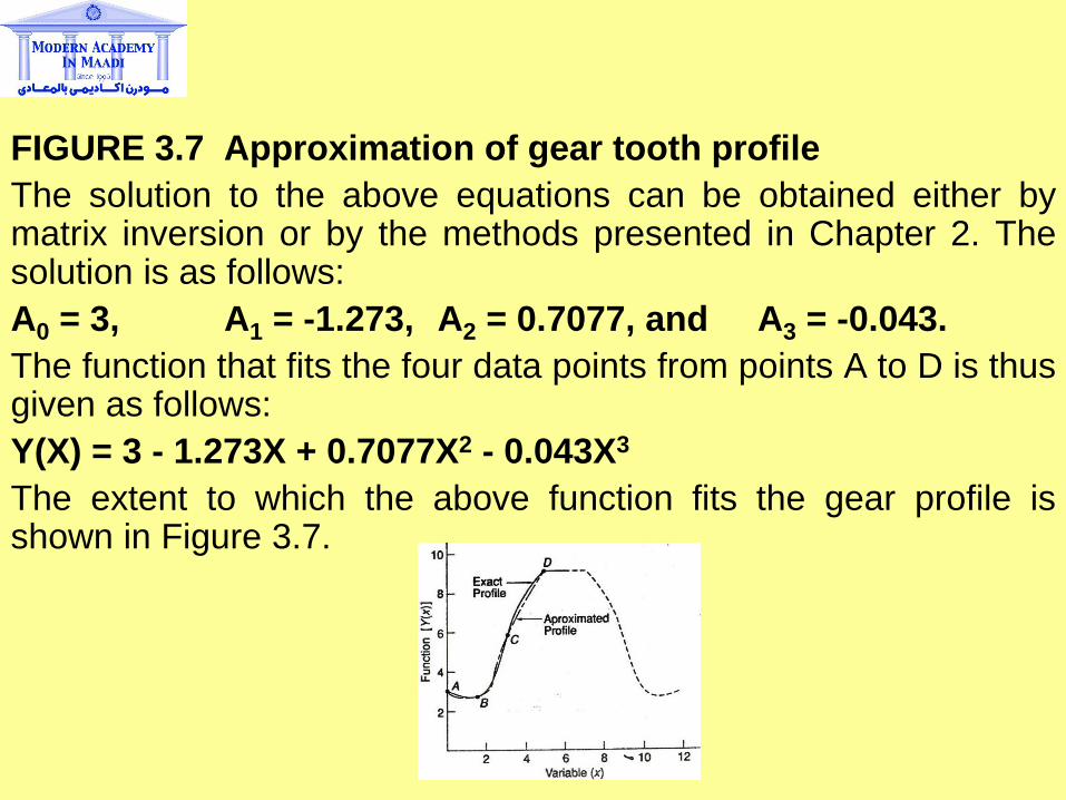
FIGURE 3.7 Approximation of gear tooth profile

The solution to the above equations can be obtained either by matrix inversion or by the methods presented in Chapter 2. The solution is as follows:

A0 = 3, A1 = -1.273, A2 = 0.7077, and A3 = -0.043.

The function that fits the four data points from points A to D is thus given as follows:

Y(X) = 3 - 1.273X + 0.7077X2 - 0.043X3

The extent to which the above function fits the gear profile is shown in Figure 3.7.

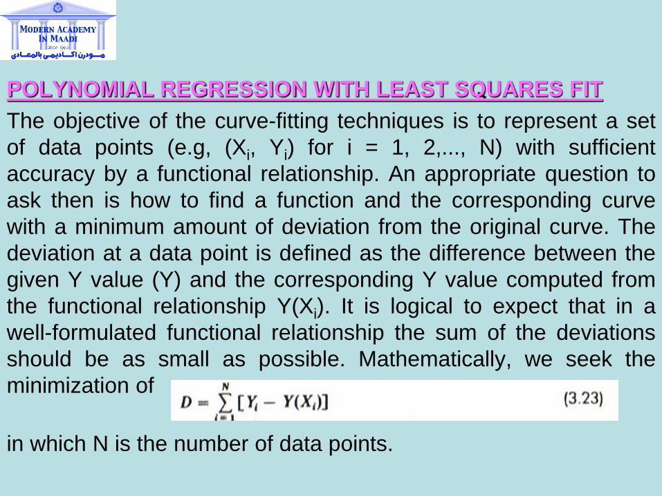
POLYNOMIAL REGRESSION WITH LEAST SQUARES FIT

The objective of the curve-fitting techniques is to represent a set

of data points (e.g, (Xi, Yi) for i = 1, 2,..., N) with sufficient

accuracy by a functional relationship. An appropriate question to

ask then is how to find a function and the corresponding curve

with a minimum amount of deviation from the original curve. The

deviation at a data point is defined as the difference between the

given Y value (Y) and the corresponding Y value computed from

the functional relationship Y(Xi). It is logical to expect that in a

well-formulated functional relationship the sum of the deviations

should be as small as possible. Mathematically, we seek the

minimization of

in which N is the number of data points.

Two major deficiencies exist in equation (3.23): (1) it does not

provide for the computation of absolute deviations, and (2) the

expression in equation (3.23), being a function of the first order,

cannot be differentiated to solve for the minimum value. An

expression for the deviation that is free of these deficiencies takes

the following form:

The function Y(X) in equation (3.24) can be expressed in many

different forms. A common choice is a polynomial similar to that

shown in equation (3.22). On substituting Y(X) from equation

(3.22) into equation (3.24), the following expression for the error

function is obtained:

Since equation (3.25) is a linear equation, the minimization of D

requires that

from which one may derive n linear algebraic equations to

solve for the coefficients A0, A1.... An.

The procedure described above involves the minimization of

the sum of the squares of the deviations. It is thus usually

referred to as the least squares method. The least squares

method gives better results than does the polynomial fitting

method when

N >n+1.

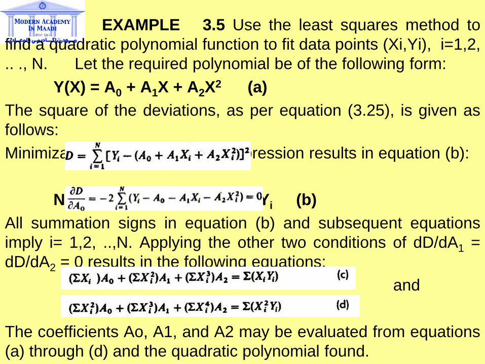
EXAMPLE 3.5 Use the least squares method to

find a quadratic polynomial function to fit data points (Xi,Yi), i=1,2,

.. ., N. Let the required polynomial be of the following form:

Y(X) = A0 + A1X + A2X2 (a)

The square of the deviations, as per equation (3.25), is given as

follows:

Minimization of D in the above expression results in equation (b):

NA0 + (SXi)Ai + (SXi2 )A2 = SYi (b)

All summation signs in equation (b) and subsequent equations

imply i= 1,2, ..,N. Applying the other two conditions of dD/dA1 =

dD/dA2 = 0 results in the following equations:

and

The coefficients Ao, A1, and A2 may be evaluated from equations

(a) through (d) and the quadratic polynomial found.

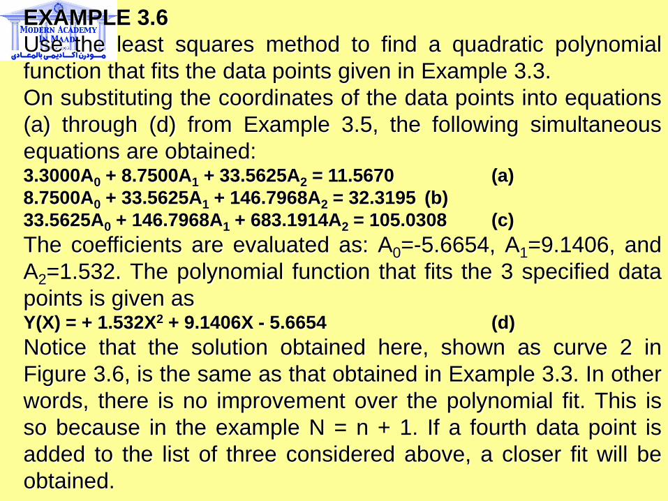
EXAMPLE 3.6

Use the least squares method to find a quadratic polynomial

function that fits the data points given in Example 3.3.

On substituting the coordinates of the data points into equations

(a) through (d) from Example 3.5, the following simultaneous

equations are obtained: 3.3000A0 + 8.7500A1 + 33.5625A2 = 11.5670 (a)

8.7500A0 + 33.5625A1 + 146.7968A2 = 32.3195 (b)

33.5625A0 + 146.7968A1 + 683.1914A2 = 105.0308 (c)

The coefficients are evaluated as: A0=-5.6654, A1=9.1406, and

A2=1.532. The polynomial function that fits the 3 specified data

points is given as Y(X) = + 1.532X2 + 9.1406X - 5.6654 (d)

Notice that the solution obtained here, shown as curve 2 in

Figure 3.6, is the same as that obtained in Example 3.3. In other

words, there is no improvement over the polynomial fit. This is

so because in the example N = n + 1. If a fourth data point is

added to the list of three considered above, a closer fit will be

obtained.

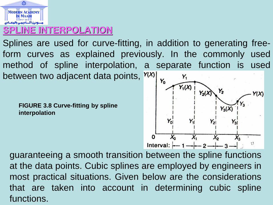
SPLINE INTERPOLATION

Splines are used for curve-fitting, in addition to generating free-

form curves as explained previously. In the commonly used

method of spline interpolation, a separate function is used

between two adjacent data points,

FIGURE 3.8 Curve-fitting by spline

interpolation

guaranteeing a smooth transition between the spline functions

at the data points. Cubic splines are employed by engineers in

most practical situations. Given below are the considerations

that are taken into account in determining cubic spline

functions.

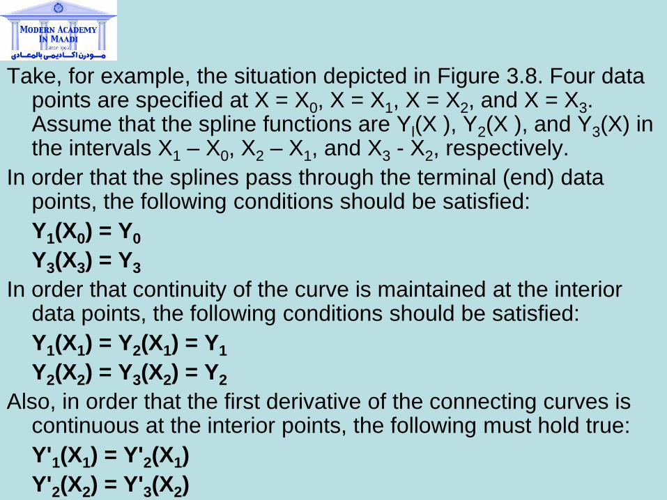
Take, for example, the situation depicted in Figure 3.8. Four data points are specified at X = X0, X = X1, X = X2, and X = X3. Assume that the spline functions are Yl(X ), Y2(X ), and Y3(X) in the intervals X1 – X0, X2 – X1, and X3 - X2, respectively.

In order that the splines pass through the terminal (end) data points, the following conditions should be satisfied:

Y1(X0) = Y0

Y3(X3) = Y3

In order that continuity of the curve is maintained at the interior data points, the following conditions should be satisfied:

Y1(X1) = Y2(X1) = Y1

Y2(X2) = Y3(X2) = Y2

Also, in order that the first derivative of the connecting curves is continuous at the interior points, the following must hold true:

Y'1(X1) = Y'2(X1)

Y'2(X2) = Y'3(X2)

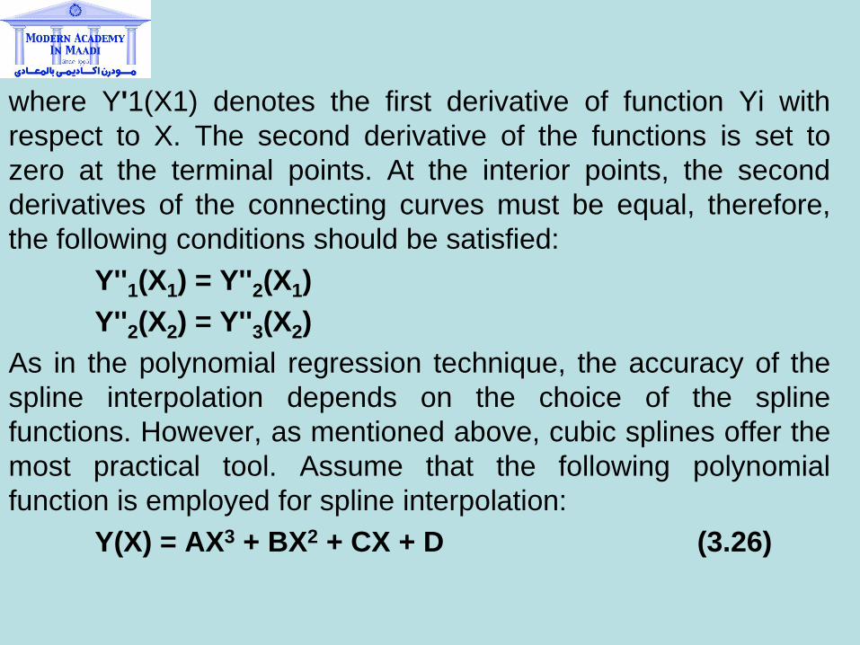
where Y'1(X1) denotes the first derivative of function Yi with

respect to X. The second derivative of the functions is set to

zero at the terminal points. At the interior points, the second

derivatives of the connecting curves must be equal, therefore,

the following conditions should be satisfied:

Y''1(X1) = Y''2(X1)

Y''2(X2) = Y''3(X2)

As in the polynomial regression technique, the accuracy of the

spline interpolation depends on the choice of the spline

functions. However, as mentioned above, cubic splines offer the

most practical tool. Assume that the following polynomial

function is employed for spline interpolation:

Y(X) = AX3 + BX2 + CX + D (3.26)

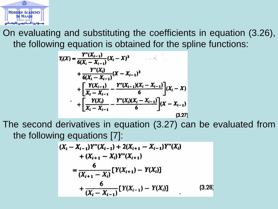
On evaluating and substituting the coefficients in equation (3.26),

the following equation is obtained for the spline functions:

The second derivatives in equation (3.27) can be evaluated from

the following equations [7]:

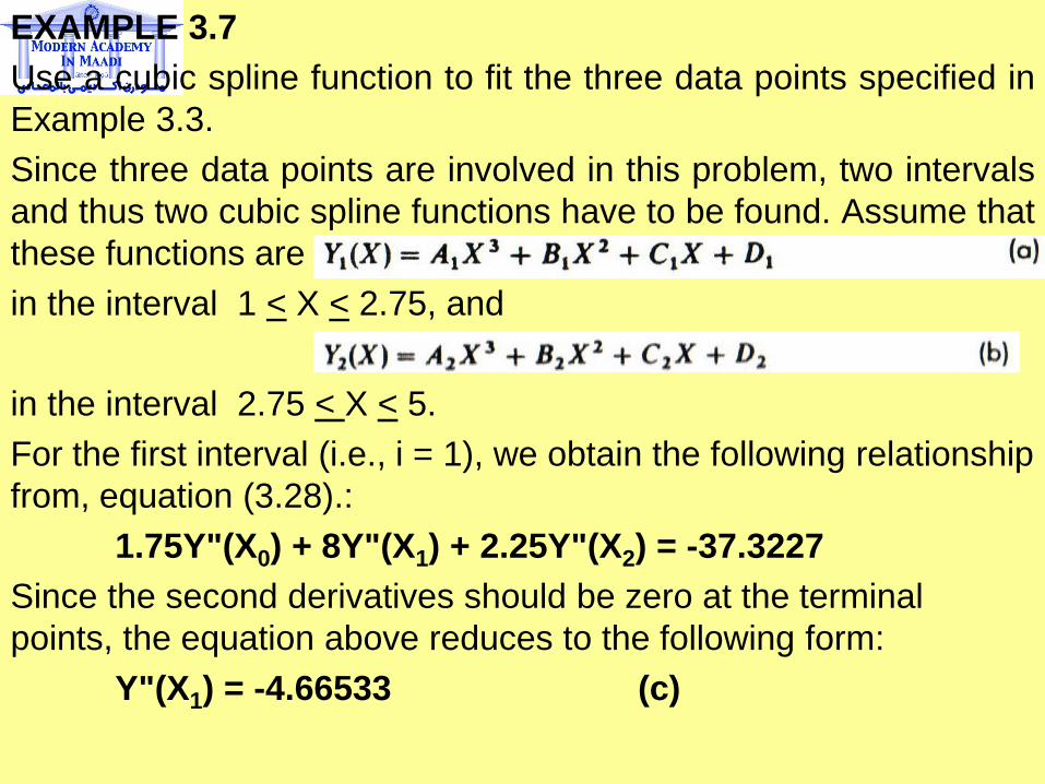
EXAMPLE 3.7

Use a cubic spline function to fit the three data points specified in

Example 3.3.

Since three data points are involved in this problem, two intervals

and thus two cubic spline functions have to be found. Assume that

these functions are

in the interval 1 < X < 2.75, and

in the interval 2.75 < X < 5.

For the first interval (i.e., i = 1), we obtain the following relationship

from, equation (3.28).:

1.75Y"(X0) + 8Y"(X1) + 2.25Y"(X2) = -37.3227

Since the second derivatives should be zero at the terminal

points, the equation above reduces to the following form:

Y"(X1) = -4.66533 (c)

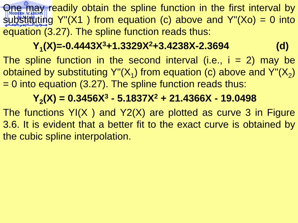
One may readily obtain the spline function in the first interval by

substituting Y"(X1 ) from equation (c) above and Y"(Xo) = 0 into

equation (3.27). The spline function reads thus:

Y1(X)=-0.4443X3+1.3329X2+3.4238X-2.3694 (d)

The spline function in the second interval (i.e., i = 2) may be

obtained by substituting Y"(X1) from equation (c) above and Y"(X2)

= 0 into equation (3.27). The spline function reads thus:

Y2(X) = 0.3456X3 - 5.1837X2 + 21.4366X - 19.0498

The functions YI(X ) and Y2(X) are plotted as curve 3 in Figure

3.6. It is evident that a better fit to the exact curve is obtained by

the cubic spline interpolation.

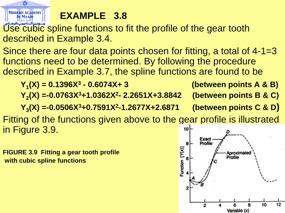
EXAMPLE 3.8

Use cubic spline functions to fit the profile of the gear tooth described in Example 3.4.

Since there are four data points chosen for fitting, a total of 4-1=3 functions need to be determined. By following the procedure described in Example 3.7, the spline functions are found to be

Y1(X) = 0.1396X3 - 0.6074X+ 3 (between points A & B)

Y2(X) =-0.0763X3+1.0362X2- 2.2651X+3.8842 (between points B & C)

Y3(X) =-0.0506X3+0.7591X2-1.2677X+2.6871 (between points C & D)

Fitting of the functions given above to the gear profile is illustrated in Figure 3.9.

FIGURE 3.9 Fitting a gear tooth profile

with cubic spline functions

3.4 Algorithms for Raster-Scan Graphics Now, the raster-scan technique is the most commonly used image display technique in computer graphics. In a raster-scan display, the intensity of each phosphor dot (picture element, pel, or pixel) is controlled separately, whether or not it contains any details of the graphics image. The image is generated on the display screen by scanning one line (of pixels) at a time, and each horizontal tine of pixels is referred to as a raster line. Most of the raster graphics display devices are operated through a frame buffer. A frame buffer consists of a large memory bank. In the simple monochrome display, the buffer contains one memory bit for each picture element in the raster display device. Thus, if there are 640 x 400 pixels on the display device (screen), the buffer contains the same number (i.e., 256,000) of memory bits in a single bit-plane. . The memory bits have binary values of either a 0 or a l. A zero value in the memory corresponds to an unlit pixel, and 1 corresponds to a lighted pixel. If there are n bit-planes in the buffer (each having the same size memory), the binary value corresponding to each pixel from each plane is loaded into a register and the values summed up. These values are then interpreted as intensity values. Ob-viously, in an n bit-plane buffer, each pixel may have 2n levels of intensity.

By varying the values of intensity within an image, a

shading effect (called a gray scale) is produced in a monochrome

composition.

For color graphics displays, there are at least 3 bit-planes (corre-

sponding to the 3 basic colors-red, green, and blue) in the frame

buffer. Each bit-plane drives a different electron color gun. By

turning on 1, 2, or all 3 guns (23 =), 8 different colors may be

produced at each pixel. By providing more than one bit-plane

corresponding to each color, display intensity of the primary colors

is individually controlled, Thus, if there are eight bit-planes for

each color, 28 shades may be produced. As explained in Chapter

1, by mixing these colors together, a total of 28x3=16,777,216

different colors can be produced.

From the above discussion, it is clear that for creating the image

of any vector, character, or solid area, a dot pattern (mask) must

be determined. The process of obtaining the dot pattern is known

as scan conversion.

In 3D graphics, where several solid areas may be involved in one

image, the priority of each area should be determined. The

priorities of the areas are used in ascertaining which areas

obscure other areas. Thus, the concept of priority is useful in

hidden surface removal algorithms, described in the next chapter.

For shaded images, a shading rule is required. By means of

appropriate shading rules, it is possible to recreate surface texture

and convey a sense of depth. In the following two sections,

algorithms for scan conversion are discussed. Shading techniques

such as those developed by Phong and Gouraud have not been

included due to space limitation.

3.5 Algorithms for Scan Conversion

STRAIGHT LINES

Equations (3.1) and (3.2) are parametric equations for straight lines. A line can thus be scan converted by finding the address of each pixel that falls on or near the line. The drawback of this approach, however, is that the calculations involve floating point (or binary fractions) calculations. Frequent rounding is thus required. An algorithm suggested by Bresenham uses integer arithmetic. This algorithm is efficient and fast, and is therefore quite popular.

RECTANGLES

A rectangle can be scan converted quite easily if its sides run along the scan lines. Let's assume that the coordinates of the lower left corner of a rectangle are (l,2) and that the rectangle is four pixels in height and five pixels in width. See Figure 3.10. It is obvious that the pixels in columns 1 through 5 belonging to rows 2 through 5 must be illuminated for a solid area representation of the rectangle. The scan conversion algorithm should therefore allocate the intensity of the rectangle to these pixels and set the intensity everywhere else on the display equal to the background value.

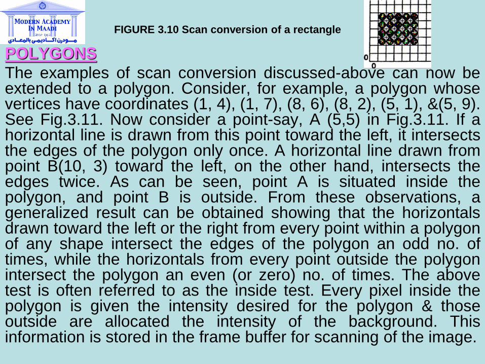
POLYGONS

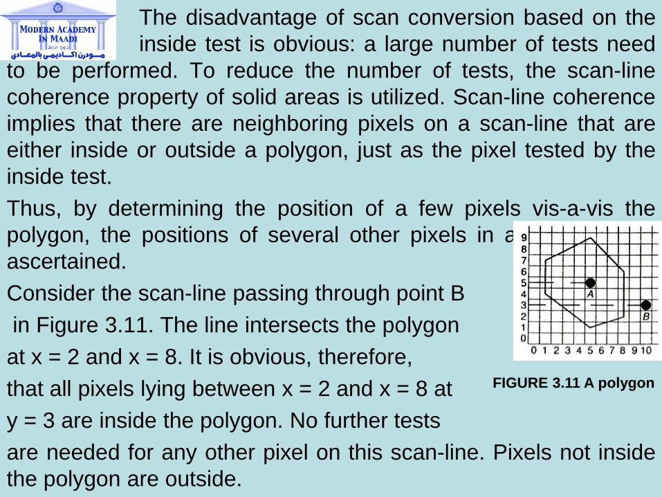
The examples of scan conversion discussed-above can now be extended to a polygon. Consider, for example, a polygon whose vertices have coordinates (1, 4), (1, 7), (8, 6), (8, 2), (5, 1), &(5, 9). See Fig.3.11. Now consider a point-say, A (5,5) in Fig.3.11. If a horizontal line is drawn from this point toward the left, it intersects the edges of the polygon only once. A horizontal line drawn from point B(10, 3) toward the left, on the other hand, intersects the edges twice. As can be seen, point A is situated inside the polygon, and point B is outside. From these observations, a generalized result can be obtained showing that the horizontals drawn toward the left or the right from every point within a polygon of any shape intersect the edges of the polygon an odd no. of times, while the horizontals from every point outside the polygon intersect the polygon an even (or zero) no. of times. The above test is often referred to as the inside test. Every pixel inside the polygon is given the intensity desired for the polygon & those outside are allocated the intensity of the background. This information is stored in the frame buffer for scanning of the image.

FIGURE 3.10 Scan conversion of a rectangle

The disadvantage of scan conversion based on the

inside test is obvious: a large number of tests need

to be performed. To reduce the number of tests, the scan-line

coherence property of solid areas is utilized. Scan-line coherence

implies that there are neighboring pixels on a scan-line that are

either inside or outside a polygon, just as the pixel tested by the

inside test.

Thus, by determining the position of a few pixels vis-a-vis the

polygon, the positions of several other pixels in a row are also

ascertained.

Consider the scan-line passing through point B

in Figure 3.11. The line intersects the polygon

at x = 2 and x = 8. It is obvious, therefore,

that all pixels lying between x = 2 and x = 8 at

y = 3 are inside the polygon. No further tests

are needed for any other pixel on this scan-line. Pixels not inside

the polygon are outside.

FIGURE 3.11 A polygon

Thus, by considering the scan-line coherence, the positions of all pixels on a horizontal line with respect to a given polygon are determined by a single test. Using the inside test scheme, many more tests (say, 640 or 720 depending on the resolution of the screen) would have been necessary, resulting in a much longer computation time. A popular algorithm that uses the scan-line coherence property is the YX' Algorithm [12].

Another form of coherence is utilized for reducing the effort required for scan conversion still further. The method, as shown below, obviates the need for determining the points of intersection of an edge with all horizontals. Also, the points of intersection are determined recursively. This other type of coherence is called edge coherence. In edge coherence it is assumed that if the ith scan-line intersects an edge, it is probable that the i + Ith scan-line also intersects the same edge. If the point of intersection of the ith scan-line has coordinates (x,, y;), then the point of intersection, if there is one, with the i + Ith scan-line will have coordinates

(xi+1 , yi+1) _ (xi + x, yi + 1) (3.29)

where x is the change in x for any unit change in

the y of the edge. x may be readily determined

from the slope of the edge. From the values obtained from

equation (3.29) and the coordinates of the end points of the

particular edge, it is easy to check whether an intersection is

possible. If no intersection is indicated, no further test is

performed on the edge. A popular algorithm based on edge

coherence is the Y-X Algorithm.

3.6 Two-Dimensional Transformations: Homogeneous

Coordinates

Thus far, we have discussed some methods that are commonly

employed for producing two-dimensional images from a given set

of data. The computer, however, provides us with the power to

view these images in a variety of ways. Images may be enlarged,

reduced, moved around (translated), or rotated using geometric

transformations implemented through transformation matrices.

There are different transformation matrices for performing different

types of imago manipulation. The structure of these matrices is

described later.

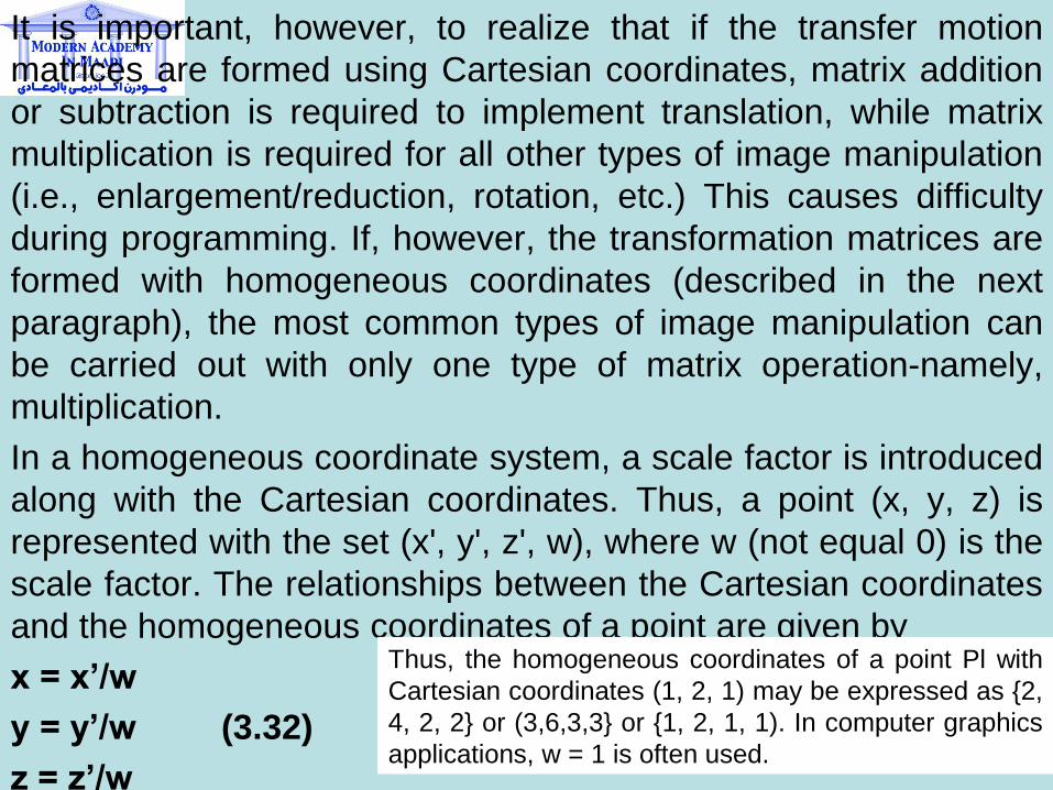
It is important, however, to realize that if the transfer motion

matrices are formed using Cartesian coordinates, matrix addition

or subtraction is required to implement translation, while matrix

multiplication is required for all other types of image manipulation

(i.e., enlargement/reduction, rotation, etc.) This causes difficulty

during programming. If, however, the transformation matrices are

formed with homogeneous coordinates (described in the next

paragraph), the most common types of image manipulation can

be carried out with only one type of matrix operation-namely,

multiplication.

In a homogeneous coordinate system, a scale factor is introduced

along with the Cartesian coordinates. Thus, a point (x, y, z) is

represented with the set (x', y', z', w), where w (not equal 0) is the

scale factor. The relationships between the Cartesian coordinates

and the homogeneous coordinates of a point are given by

x = x’/w

y = y’/w (3.32)

z = z’/w

Thus, the homogeneous coordinates of a point Pl with

Cartesian coordinates (1, 2, 1) may be expressed as {2,

4, 2, 2} or (3,6,3,3} or {1, 2, 1, 1). In computer graphics

applications, w = 1 is often used.

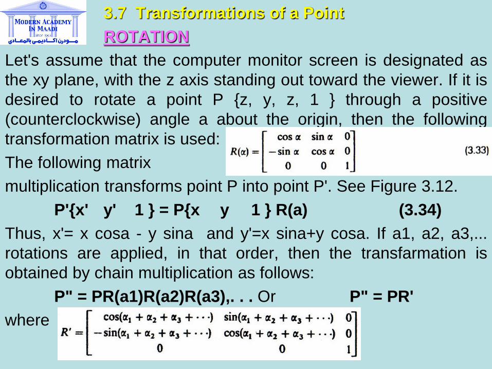
3.7 Transformations of a Point

ROTATION

Let's assume that the computer monitor screen is designated as

the xy plane, with the z axis standing out toward the viewer. If it is

desired to rotate a point P {z, y, z, 1 } through a positive

(counterclockwise) angle a about the origin, then the following

transformation matrix is used:

The following matrix

multiplication transforms point P into point P'. See Figure 3.12.

P'{x' y' 1 } = P{x y 1 } R(a) (3.34)

Thus, x'= x cosa - y sina and y'=x sina+y cosa. If a1, a2, a3,...

rotations are applied, in that order, then the transfarmation is

obtained by chain multiplication as follows:

P" = PR(a1)R(a2)R(a3),. . . Or P" = PR'

where

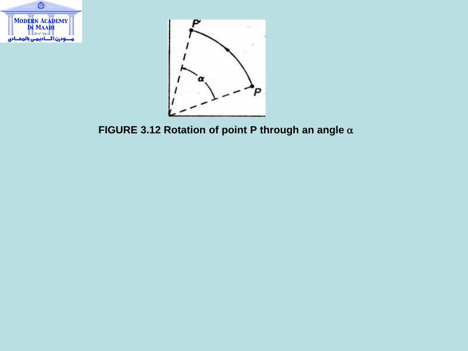
FIGURE 3.12 Rotation of point P through an angle a

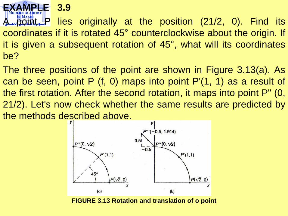
EXAMPLE 3.9

A point P lies originally at the position (21/2, 0). Find its

coordinates if it is rotated 45° counterclockwise about the origin. If

it is given a subsequent rotation of 45°, what will its coordinates

be?

The three positions of the point are shown in Figure 3.13(a). As

can be seen, point P (f, 0) maps into point P'(1, 1) as a result of

the first rotation. After the second rotation, it maps into point P" (0,

21/2). Let's now check whether the same results are predicted by

the methods described above.

FIGURE 3.13 Rotation and translation of o point

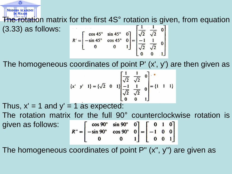
The rotation matrix for the first 4S° rotation is given, from equation

(3.33) as follows:

The homogeneous coordinates of point P' (x', y') are then given as

Thus, x' = 1 and y' = 1 as expected:

The rotation matrix for the full 90° counterclockwise rotation is

given as follows:

The homogeneous coordinates of point P" (x", y") are given as

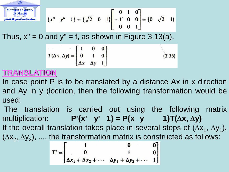
Thus, x" = 0 and y" = f, as shown in Figure 3.13(a).

TRANSLATION

In case point P is to be translated by a distance Ax in x direction

and Ay in y (locriion, then the following transformation would be

used:

The translation is carried out using the following matrix

multiplication: P'{x' y' 1} = P{x y 1}T(x, y)

If the overall translation takes place in several steps of (x1, y1),

(x2, y2), .... the transformation matrix is constructed as follows:

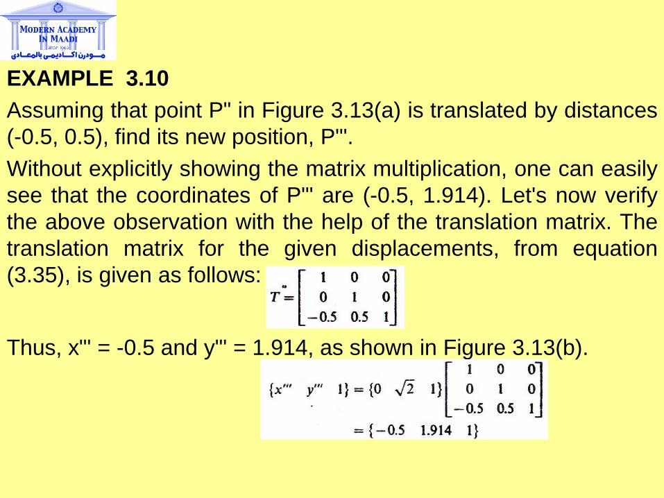
EXAMPLE 3.10

Assuming that point P" in Figure 3.13(a) is translated by distances

(-0.5, 0.5), find its new position, P"'.

Without explicitly showing the matrix multiplication, one can easily

see that the coordinates of P"' are (-0.5, 1.914). Let's now verify

the above observation with the help of the translation matrix. The

translation matrix for the given displacements, from equation

(3.35), is given as follows:

Thus, x"' = -0.5 and y"' = 1.914, as shown in Figure 3.13(b).

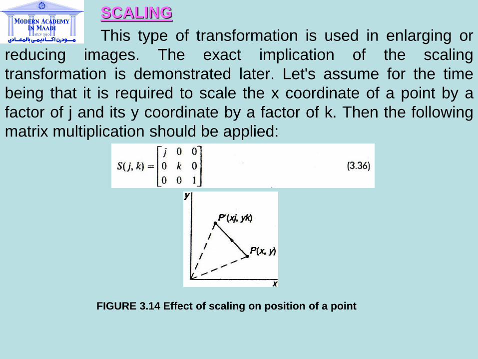
SCALING

This type of transformation is used in enlarging or

reducing images. The exact implication of the scaling

transformation is demonstrated later. Let's assume for the time

being that it is required to scale the x coordinate of a point by a

factor of j and its y coordinate by a factor of k. Then the following

matrix multiplication should be applied:

FIGURE 3.14 Effect of scaling on position of a point

And, as a result of the following transformation, point

P is mapped into paint P, as shown in Figure 3.14:

P'{x' y' 1} = P{x y 1}S( j, k)

where

x' = xj (3.37)

y'= yk (3.38)

If successive scaling of (j1 , k1), (j2, k2), . . . , is applied, the

combined scaling matrix is given as follows:

REFLECTION

Post multiplication of the homogeneous coordinates of a point with

a matrix of the form shown in equation (3.39) results in the

reflection of the point about the x axis.

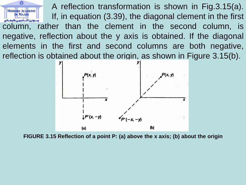
A reflection transformation is shown in Fig.3.15(a).

If, in equation (3.39), the diagonal clement in the first

column, rather than the clement in the second column, is

negative, reflection about the y axis is obtained. If the diagonal

elements in the first and second columns are both negative,

reflection is obtained about the origin, as shown in Figure 3.15(b).

FIGURE 3.15 Reflection of a point P: (a) above the x axis; (b) about the origin

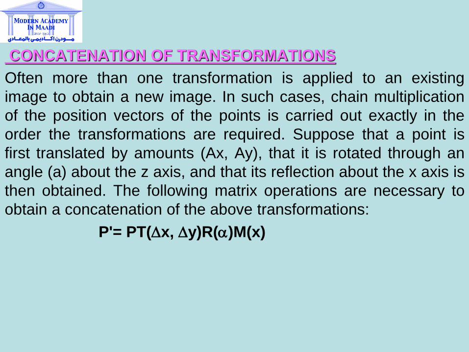
CONCATENATION OF TRANSFORMATIONS

Often more than one transformation is applied to an existing

image to obtain a new image. In such cases, chain multiplication

of the position vectors of the points is carried out exactly in the

order the transformations are required. Suppose that a point is

first translated by amounts (Ax, Ay), that it is rotated through an

angle (a) about the z axis, and that its reflection about the x axis is

then obtained. The following matrix operations are necessary to

obtain a concatenation of the above transformations:

P'= PT(x, y)R(a)M(x)

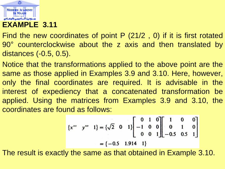
EXAMPLE 3.11

Find the new coordinates of point P (21/2 , 0) if it is first rotated

90° counterclockwise about the z axis and then translated by

distances (-0.5, 0.5).

Notice that the transformations applied to the above point are the

same as those applied in Examples 3.9 and 3.10. Here, however,

only the final coordinates are required. It is advisable in the

interest of expediency that a concatenated transformation be

applied. Using the matrices from Examples 3.9 and 3.10, the

coordinates are found as follows:

The result is exactly the same as that obtained in Example 3.10.

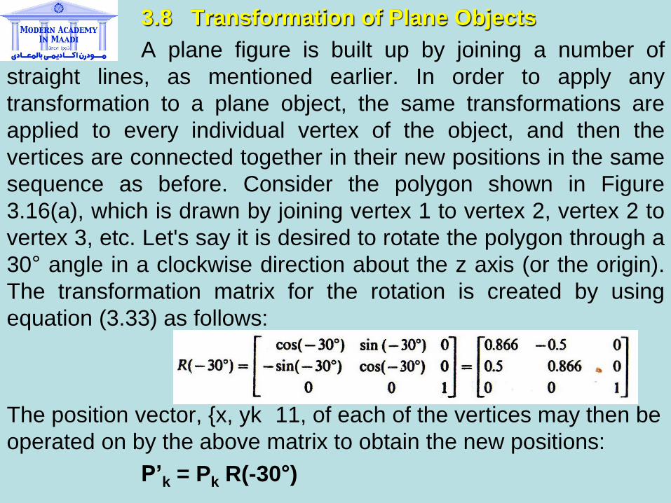
3.8 Transformation of Plane Objects

A plane figure is built up by joining a number of

straight lines, as mentioned earlier. In order to apply any

transformation to a plane object, the same transformations are

applied to every individual vertex of the object, and then the

vertices are connected together in their new positions in the same

sequence as before. Consider the polygon shown in Figure

3.16(a), which is drawn by joining vertex 1 to vertex 2, vertex 2 to

vertex 3, etc. Let's say it is desired to rotate the polygon through a

30° angle in a clockwise direction about the z axis (or the origin).

The transformation matrix for the rotation is created by using

equation (3.33) as follows:

The position vector, {x, yk 11, of each of the vertices may then be

operated on by the above matrix to obtain the new positions:

P’k = Pk R(-30°)

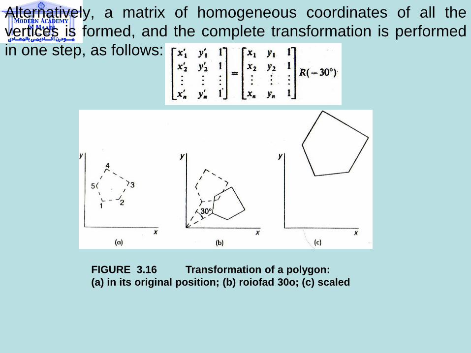
Alternatively, a matrix of homogeneous coordinates of all the

vertices is formed, and the complete transformation is performed

in one step, as follows:

FIGURE 3.16 Transformation of a polygon:

(a) in its original position; (b) roiofad 30o; (c) scaled

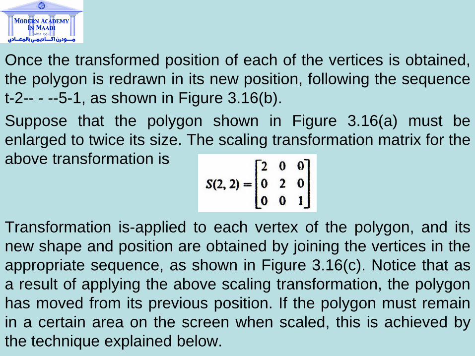
Once the transformed position of each of the vertices is obtained,

the polygon is redrawn in its new position, following the sequence

t-2-- - --5-1, as shown in Figure 3.16(b).

Suppose that the polygon shown in Figure 3.16(a) must be

enlarged to twice its size. The scaling transformation matrix for the

above transformation is

Transformation is-applied to each vertex of the polygon, and its

new shape and position are obtained by joining the vertices in the

appropriate sequence, as shown in Figure 3.16(c). Notice that as

a result of applying the above scaling transformation, the polygon

has moved from its previous position. If the polygon must remain

in a certain area on the screen when scaled, this is achieved by

the technique explained below.

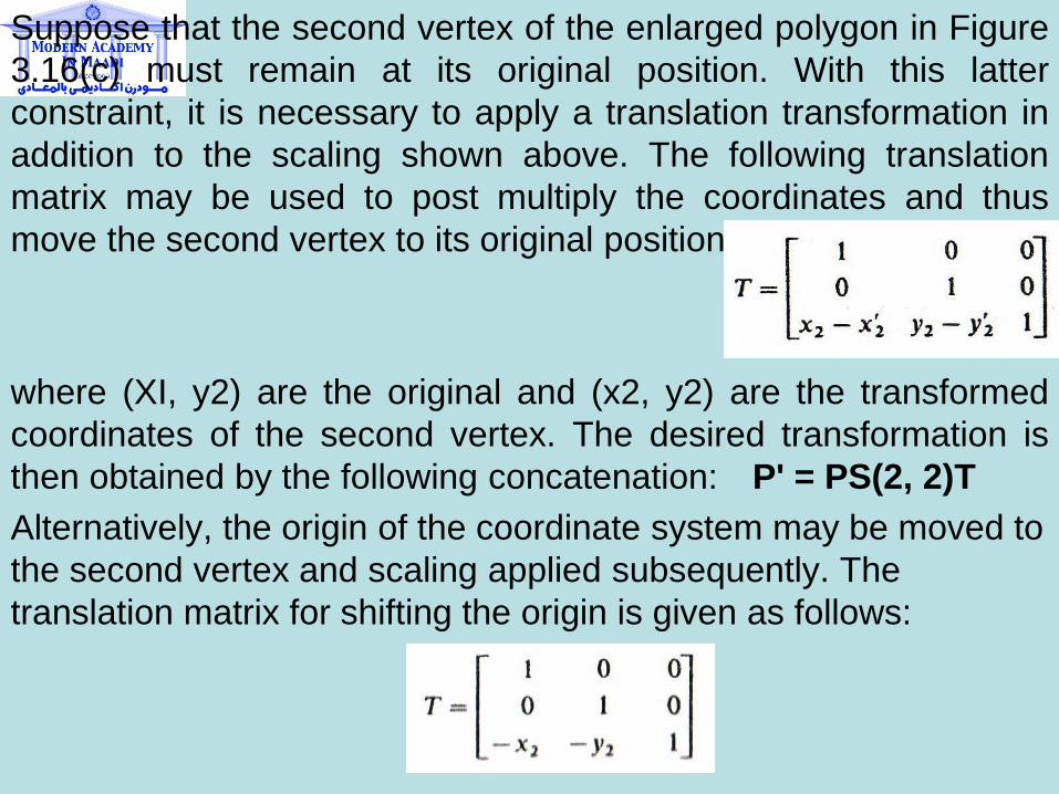
Suppose that the second vertex of the enlarged polygon in Figure

3.16(c) must remain at its original position. With this latter

constraint, it is necessary to apply a translation transformation in

addition to the scaling shown above. The following translation

matrix may be used to post multiply the coordinates and thus

move the second vertex to its original position

where (XI, y2) are the original and (x2, y2) are the transformed

coordinates of the second vertex. The desired transformation is

then obtained by the following concatenation: P' = PS(2, 2)T

Alternatively, the origin of the coordinate system may be moved to

the second vertex and scaling applied subsequently. The

translation matrix for shifting the origin is given as follows:

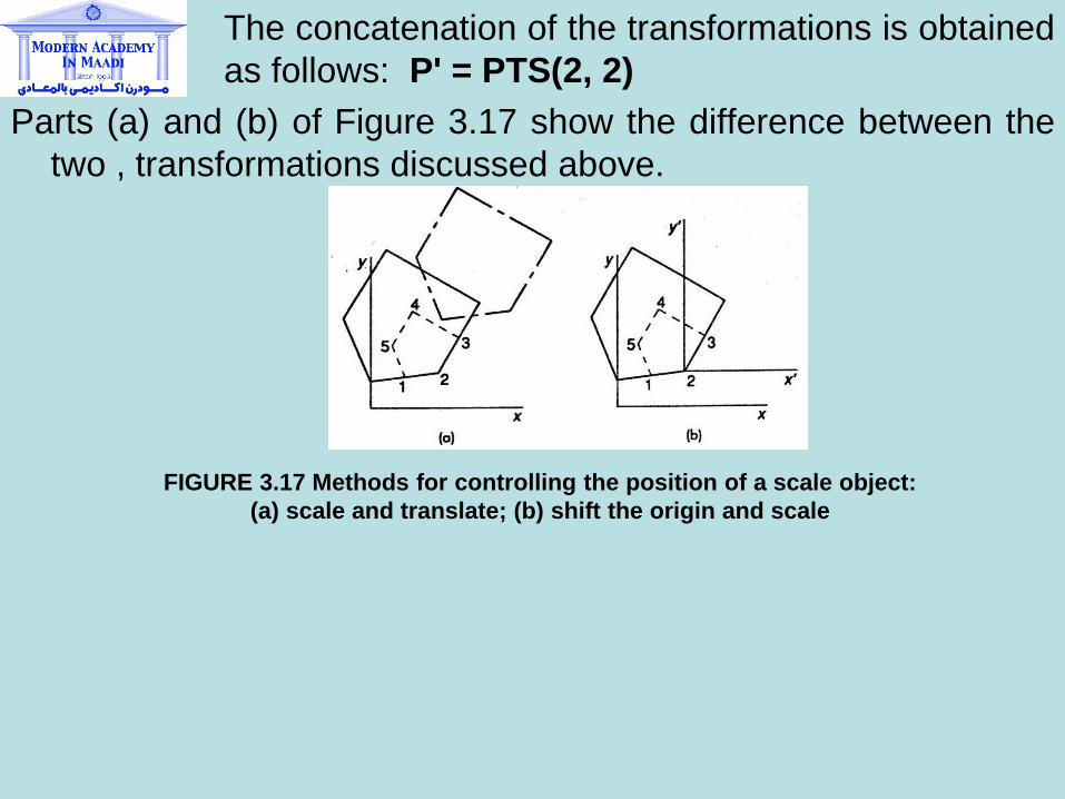
The concatenation of the transformations is obtained

as follows: P' = PTS(2, 2)

Parts (a) and (b) of Figure 3.17 show the difference between the

two , transformations discussed above.

FIGURE 3.17 Methods for controlling the position of a scale object:

(a) scale and translate; (b) shift the origin and scale

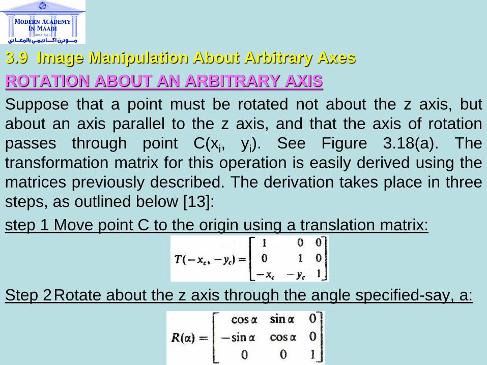
3.9 Image Manipulation About Arbitrary Axes

ROTATION ABOUT AN ARBITRARY AXIS

Suppose that a point must be rotated not about the z axis, but

about an axis parallel to the z axis, and that the axis of rotation

passes through point C(xi, yi). See Figure 3.18(a). The

transformation matrix for this operation is easily derived using the

matrices previously described. The derivation takes place in three

steps, as outlined below [13]:

step 1 Move point C to the origin using a translation matrix:

Step 2 Rotate about the z axis through the angle specified-say, a:

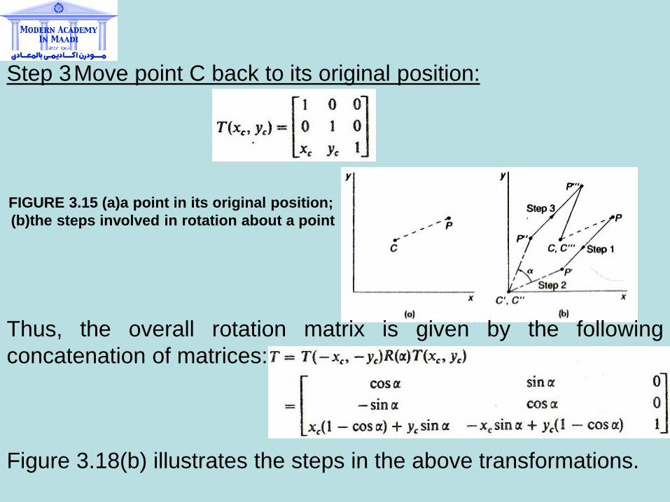
Step 3 Move point C back to its original position:

FIGURE 3.15 (a)a point in its original position;

(b)the steps involved in rotation about a point

Thus, the overall rotation matrix is given by the following

concatenation of matrices:

Figure 3.18(b) illustrates the steps in the above transformations.

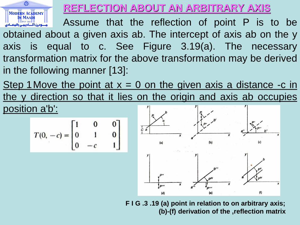
REFLECTION ABOUT AN ARBITRARY AXIS

Assume that the reflection of point P is to be

obtained about a given axis ab. The intercept of axis ab on the y

axis is equal to c. See Figure 3.19(a). The necessary

transformation matrix for the above transformation may be derived

in the following manner [13]:

Step 1 Move the point at x = 0 on the given axis a distance -c in

the y direction so that it lies on the origin and axis ab occupies

position a'b':

F I G .3 .19 (a) point in relation to on arbitrary axis;

(b)-(f) derivation of the ,reflection matrix

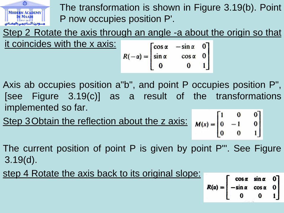
The transformation is shown in Figure 3.19(b). Point

P now occupies position P'.

Step 2 Rotate the axis through an angle -a about the origin so that

it coincides with the x axis:

Axis ab occupies position a"b", and point P occupies position P",

[see Figure 3.19(c)] as a result of the transformations

implemented so far.

Step 3 Obtain the reflection about the z axis:

The current position of point P is given by point P"'. See Figure

3.19(d).

step 4 Rotate the axis back to its original slope:

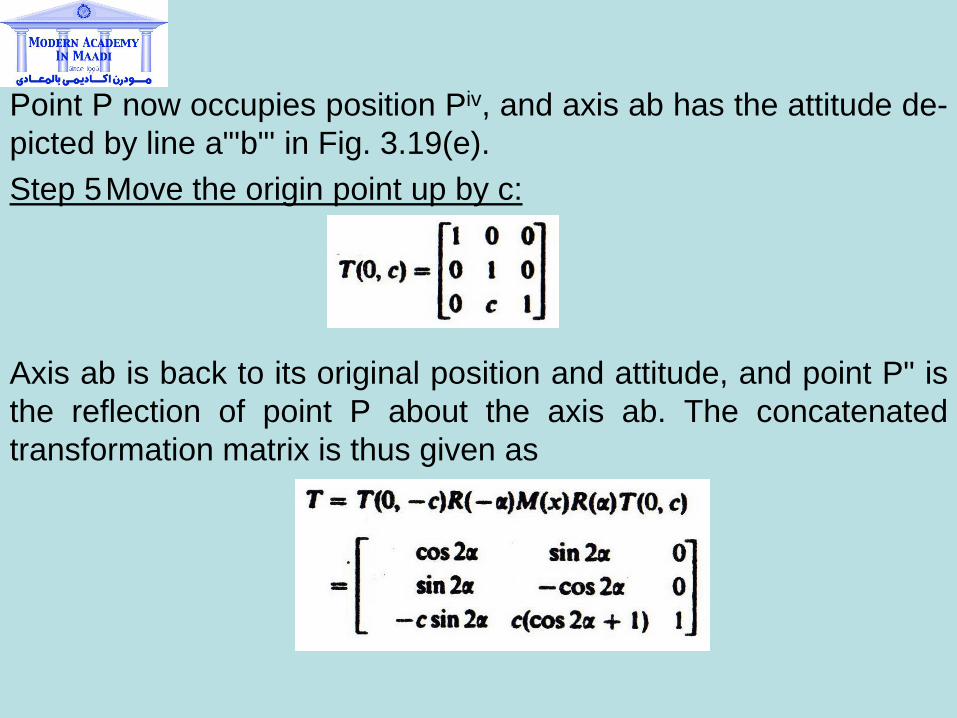
Point P now occupies position Piv, and axis ab has the attitude de-

picted by line a"'b"' in Fig. 3.19(e).

Step 5 Move the origin point up by c:

Axis ab is back to its original position and attitude, and point P" is

the reflection of point P about the axis ab. The concatenated

transformation matrix is thus given as

3.10 Graphics Packages and Graphics Standards

For application programs in a high-level language, a graphics package is required for producing (rendering) images of objects. A typical graphics package contains the following features:

Graphics primitive subroutines for points, lines, circles, symbols, and characters

Window, viewport, and clipping subroutines

Miscellaneous subroutines for entering and leaving the graphics mode, selecting colors, hard copying, etc.

Graphics packages were originally written in low-level machine language by computer hardware manufacturers and worked only on the specific computers in question. An application program that used the graphics package could thus be run only on the specific machine. This situation was unsatisfactory for developing portable programs (i.e., programs that could work on all computers and display devices). It was therefore felt that some method should be found for obviating machine dependence of graphics programs. The route taken toward this goal was the use of graphics standards.

As you are no doubt aware, English has been standardized as the language of international aviation. A pilot, therefore, flying over any territory in the world can communicate with the nearest control tower to seek help & directions. In computer programming, a similar approach was taken by standardizing FORTRAN, COBOL, Pascal, etc. Introduction of these high-level languages caused an explosion in computer utilization. What has worked in other aspects of life should work in computer graphics as well. Driven by such conviction, computer scientists in industry and academia began to develop graphics standards. In 1977 a set of specifications for graphical programming was established by the Special Interest Group on Graphics (SIGGRAPH) of the Association for Computer Machinery (ACM). These specifications were given the name CORE Graphics System (or Core). Another set of graphics standards, developed in Europe, is known as the Graphical Kernel System (GKS). The International Standard Organization (ISO) and the American National Standard Institute (ANSI) have accepted GKS as their official standard (14,153. GKS and Core consist of a no. of subroutines, which application programmers (i.e., the people who write programs as opposed to those who use somebody else's programs) may incorporate within a program for graphical images. GKS defines about 200 different subroutines.

These subroutines are independent of any programming lan-

guage. Some language bindings are also standardized, and work

is continuing on more. Language bindings allow the programmer

to call the GKS subroutines from various high-level programming

languages. Once all language bindings have been standardized, it

will be possible to call any GKS graphics subroutine from any

high-level language.

Core is a full three-dimensional graphics system. GKS is at the

moment a two-dimensional system. A draft standard-namely,

GKS-3D [16]was released in 1987 for applications involving three-

dimensional graphics. A brief discussion of GKS-3D and PHIGS,

yet another graphics standard, is given in Section 3.14.

3.11 Graphical Kernel System (GKS)

As might be expected, GKS is language and device independent.

This means that the system can be adopted for use in almost any

programming language and on almost any graphics input/output

device.

Device independence in GKS is achieved through the use of

virtual devices. A virtual device is an idealized device with defined

characteristics. In general, any commercial graphics device does

not have (lie exact characteristics of the virtual device. The

characteristics of the virtual devices, however, may be selected so

as to simulate many commercial devices.

3.12 Graphics Primitives in GKS

Four main types of graphics primitives are provided in GKS: (1)

polyline, (2) polymarker, (3) fill area, and (4) text. In the

paragraphs below, each of these primitives is described in brief;

more details may be found in specialized references.

POLYLINIE

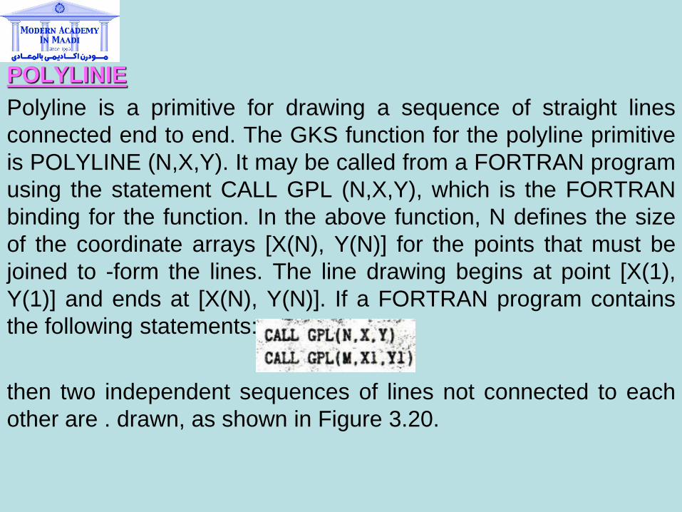
Polyline is a primitive for drawing a sequence of straight lines

connected end to end. The GKS function for the polyline primitive

is POLYLINE (N,X,Y). It may be called from a FORTRAN program

using the statement CALL GPL (N,X,Y), which is the FORTRAN

binding for the function. In the above function, N defines the size

of the coordinate arrays [X(N), Y(N)] for the points that must be

joined to -form the lines. The line drawing begins at point [X(1),

Y(1)] and ends at [X(N), Y(N)]. If a FORTRAN program contains

the following statements:

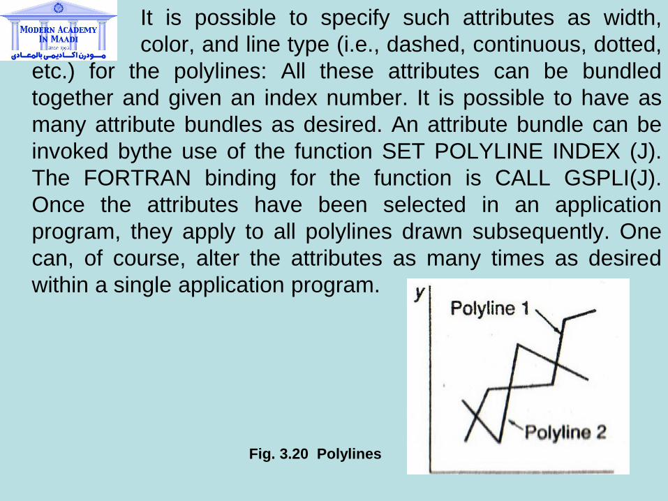
then two independent sequences of lines not connected to each

other are . drawn, as shown in Figure 3.20.

It is possible to specify such attributes as width,

color, and line type (i.e., dashed, continuous, dotted,

etc.) for the polylines: All these attributes can be bundled

together and given an index number. It is possible to have as

many attribute bundles as desired. An attribute bundle can be

invoked bythe use of the function SET POLYLINE INDEX (J).

The FORTRAN binding for the function is CALL GSPLI(J).

Once the attributes have been selected in an application

program, they apply to all polylines drawn subsequently. One

can, of course, alter the attributes as many times as desired

within a single application program.

Fig. 3.20 Polylines

POLYMARKER

At times one may wish not to connect data points, but rather to

plot them as discrete points. For such applications, function

POLYMARKER (N,X,Y) has been provided. The FORTRAN 77

binding for the polymarker is CALL GPM(N,X,Y), where N is the

number of data points and [X(N), Y(N)] are the coordinates of

those points. Attributes for the data points are selected through

the function SET POLYMARKER INDEX (N). The FORTRAN 77

binding for the above function is CALL GSPMI(N). As with the

polylines, the index number is associated with a number of

attributes that the user may select. Depending on the attributes

selected, different types of markers are drawn.