computed tomography image denoising...

i

COMPUTED TOMOGRAPHY IMAGE DENOISING BASED ON MULTI

DOSE CT IMAGE FUSION AND EXTENDED SPARSE TECHNIQUES

by

Anuyogam Venkataraman

BE, Anna University, Chennai, India, 2010

A thesis

presented to Ryerson University

in partial fulfillment of the

requirements for the degree of

Master of Applied Science

in the program of

Electrical and Computer Engineering

Toronto, Ontario, Canada, 2014

© (Anuyogam Venkataraman) 2014

ii

I hereby declare that I am the sole author of this thesis. This is a true copy of the thesis, including

any required final revisions, as accepted by my examiners.

I authorize Ryerson University to lend this thesis or dissertation to other institutions or

individuals for the purpose of scholarly research.

I further authorize Ryerson University to reproduce this thesis by photocopying or by other

means, in total or in part, at the request of other institutions or individuals for the purpose of

scholarly research.

I understand that my thesis may be made electronically available to the public.

iii

COMPUTED TOMOGRAPHY IMAGE DENOISING BASED ON MULTI

DOSE CT IMAGE FUSION AND EXTENDED SPARSE TECHNIQUES

Master of Applied Science 2014

Anuyogam Venkataraman

Electrical and Computer Engineering

Ryerson University

Abstract

With the increasing utilization of X-ray Computed Tomography (CT) in medical diagnosis, obtaining

higher quality image with lower exposure to radiation is a highly challenging task in image processing.

Sparse representation based image fusion is one of the sought after fusion techniques among the current

researchers. A novel image fusion algorithm based on focused vector detection is proposed in this thesis.

Firstly, the initial fused vector is acquired by combining common and innovative sparse components of

multi-dosage ensemble using Joint Sparse PCA fusion method utilizing an overcomplete dictionary

trained using high dose images of the same region of interest from different patients. And then, the

strongly focused vector is obtained by determining the pixels of low dose and medium dose vectors which

have high similarity with the pixels of the initial fused vector using certain quantitative metrics. Final

fused image is obtained by denoising and simultaneously integrating the strongly focused vector, initial

fused vector and source image vectors in joint sparse domain thereby preserving the edges and other

critical information needed for diagnosis. This thesis demonstrates the effectiveness of the proposed

algorithms when experimented on different images and the qualitative and quantitative results are

compared with some of the widely used image fusion methods.

iv

Acknowledgements

I would like to thank my supervisor Prof. Javad Alirezaie, for his outstanding support,

encouragement and endless patience throughout the course of my research work. It was a great

learning experience for me to complete this research under his valuable guidance. I would also

like to extend my gratitude to Dr. Paul Babyn for providing helpful insights and needful

resources without which this research work would not have been possible.

I would like to dedicate this thesis to my beloved husband who has stood by me during all my

difficult times and has been a great mental and physical support throughout my graduate studies.

I would not have been where I am today without his motivation and endurance. I also thank my

parents and sister who have always wished only the best for me. I would like to thank all my

CVIP lab friends for their timely help and especially Samira who has supported me with lots of

optimism during the tougher times and for making this journey a memorable experience.

v

TABLE OF CONTENTS

Chapter 1. Introduction ……………………………………………………………………………….1

1.1 Background………………………………………………………………………………1

1.2 Problem statement ……………………………………………………………………….2

1.3 Overview of Techniques adopted ………………………………………………………..2

1.4 Framework and Requirements …………………………………………………………...3

1.5 Major contributions……………………………………………………………………….4

1.6 Overview of the thesis ……………………………………………………………………5

Chapter 2. Sparse Representation

2.1. Introduction to Sparsity………………………………………………………………….6

2.2. Regularization…………………………………………………………………………....8

2.3. Spare Approximation…………………………………………………………………….9

2.4. Example of sparse representation and approximation…………………………………10

2.5. Uncertainty………………………………………………………………………………11

2.6. Uniqueness of sparse representation…………………………………………………….12

2.7. Necessity of sparse approximation……………………………………………………...12

2.8. Sparse coding algorithms………………………………………………………………..13

2.8.1. LASSO and Basis Pursuit………………………………………………...…………13

2.8.2. Greedy Algorithms…………………………………………………………...……...13

2.8.2.1. Matching Pursuit with Time-Frequency Dictionaries……………...……………14

2.8.2.2. Weak Matching Pursuit algorithm……………………………………...………..15

2.8.2.3. Orthogonal Matching Pursuit algorithm………………………………...……….17

2.8.2.4. Stage wise Orthogonal Matching Pursuit…………………………...…………....18

Chapter 3. Dictionaries

3.1. Comparison of analytical and adaptive dictionary….……………………..……………..21

3.2. Time-Frequency Dictionaries………………………………………………..…………...22

3.2.1. Discrete Cosine Transform ……………………………………..…………………...23

3.2.2. Overcomplete Discrete Cosine Transform………………………..………………….23

3.2.3. Overcomplete Haar Dictionary…………………………………………..…………..26

vi

3.2.4. Continuous wavelet Transform………………………………………………….….....27

3.2.5. Continuous wavelet Transform with discrete wavelet coefficients…………....….…..27

3.2.6. Discrete Wavelet Transform…………………………………………………....….….29

3.2.7. Dual Tree Complex Wavelet transform……………………………………….…....…30

3.3. Dictionary Learning……………………………………………………………….…….….30

3.3.1 Method of Optimal Directions Algorithm……………………………....….……31

3.3.2. K-SVD Algorithm……………………………………………………….….…..32

Chapter 4. Image Fusion

4.1. Introduction…………………………………………………………………………………36

4.2. Generic requirements of fusion algorithm………………………………………………….36

4.3. Preprocessing to satisfy Common Representation Format…………………………………37.

4.4. Selection methodology……………………………………………………………………...38

4.5. A brief review on area of application: Computed Tomography……………………...…….39

4.5.1. Historical Milestones of Computed Tomography…………………………………..….40

4.5.2. Working of CT………………………………………………………………………….41

4.5.3. Reconstruction methods………………………………………………………………...41

4.5.4. Computed Tomography Dose…………………………………………………………..42

4.5.5. Computed Tomography Noise…………………………………………………………..45

4.6. Fusion Methodologies………………………………………………………………………..46

4.6.1. Image fusion using multi scale approach………………………………………………..46

4.6.2. 2D-Discrete Wavelet Transform Fusion……………………………………………...…48

4.6.3. Principal Component Analysis based fusion………………………………………........51

4.7. Image Quality Measurement…………………………………………………………...…….55

Chapter 5. Proposed Methodologies

5.1. Image Fusion Using Simultaneous Controlled St-OMP……………………………………..59

5.2. Medical Image Fusion Based on Joint Sparse Method………………………………………64

5.3. Simultaneous medical image fusion and denoising using focused region in sparse domain..72

5.3.1 Dictionary learning and acquisition of initial fused image……………………………….72

5.3.2. Detection of focused region and fusion scheme…………………………………………75

Chapter 6. Results and Discussions

6.1. Implementation using Graphical User Interface………………………………………………78

6.2. Experimental setup and results of Simultaneous Controlled St-OMP………………………...80

6.3. Experimental setup and Results of Contribution II and Contribution III……………………..92

6.4. Integration of unregistered images using focused region fusion……………………...………98

vii

Chapter 7. Conclusion and Future Works

7.1. Image fusion with simultaneous controlled orthogonal matching pursuit…………………101

7.2. Image fusion with Joint Sparse Fusion……………………………………………………..102

7.3. Fusion based on focused Vector……………………………………………………………102

viii

List of Tables

Table 2.1 Pseudo algorithm of Matching Pursuit

Table 2.2 Pseudo algorithm of Weak Matching Pursuit

Table 2.3 Pseudo algorithm of Orthogonal Matching Pursuit

Table 2.4. Pseudo algorithm of Stage wise Orthogonal Matching Pursuit

Table 3.1. Pseudo algorithm of MOD dictionary learning strategy

Table 3.2. Pseudo Algorithm of KSVD Algorithm

Table 5.1. Pseudo algorithm of proposed Simultaneous Controlled St-OMP fusion

Table 5.2. Pseudo algorithm of Joint Sparse PCA fusion method

Table 6.1. Performance evaluation of proposed method for standard images quantitatively

Table 6.2. Performance evaluation of proposed method for CT images quantitatively



ix

List of Figures

Figure 1.1 Generic pixel level fusion processing chain

Figure 2.1. Depiction of sparse representation concept and the size of each matrix

Figure 2.3 Block diagram of St-OMP framework

Figure 3.1. Depiction of Simple DCT Dictionary of 16 atoms and DCT Dictionary of

64 atoms

Figure 3.2. DCT dictionary with patches

Figure 3.3. (a) DWT having one decomposition level (b) DWT having three decomposition

levels and (c) Haar Dictionary basis

Figure 3.4. Left image representing the Wavelets associated with the orientation of DTCWT and

Right image represents the Overcomplete DTCWT dictionary

Figure 4.1. Source images to be integrated: (a) Visual image (b) infrared image.

Figure 4.2. Principle of Computed Tomography


Figure 4.2. Principle of Computed Tomography

Figure.4.3. 2D Decomposition; level=3

Figure.4.4. 2D DWT Fusion framework

Figure.4.5. 2D DTCWT Fusion framework

Figure.4.6. PCA Fusion framework

Figure 5.1. Framework of proposed Simultaneous Controlled St-OMP fusion

Figure 5.2. Framework of Joint Sparse PCA fusion methodology

x

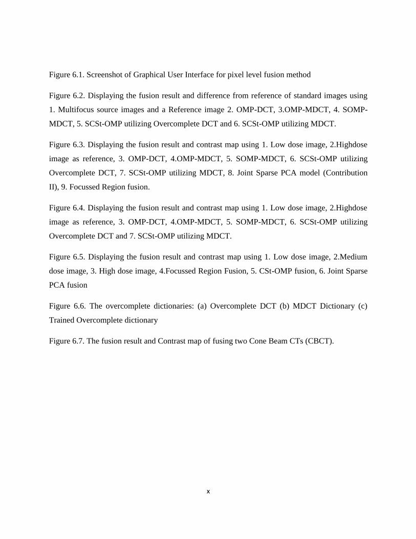
Figure 6.1. Screenshot of Graphical User Interface for pixel level fusion method

Figure 6.2. Displaying the fusion result and difference from reference of standard images using

1. Multifocus source images and a Reference image 2. OMP-DCT, 3.OMP-MDCT, 4. SOMP-

MDCT, 5. SCSt-OMP utilizing Overcomplete DCT and 6. SCSt-OMP utilizing MDCT.

Figure 6.3. Displaying the fusion result and contrast map using 1. Low dose image, 2.Highdose

image as reference, 3. OMP-DCT, 4.OMP-MDCT, 5. SOMP-MDCT, 6. SCSt-OMP utilizing

Overcomplete DCT, 7. SCSt-OMP utilizing MDCT, 8. Joint Sparse PCA model (Contribution

II), 9. Focussed Region fusion.


image as reference, 3. OMP-DCT, 4.OMP-MDCT, 5. SOMP-MDCT, 6. SCSt-OMP utilizing

Overcomplete DCT and 7. SCSt-OMP utilizing MDCT.

Figure 6.5. Displaying the fusion result and contrast map using 1. Low dose image, 2.Medium

dose image, 3. High dose image, 4.Focussed Region Fusion, 5. CSt-OMP fusion, 6. Joint Sparse

PCA fusion

Figure 6.6. The overcomplete dictionaries: (a) Overcomplete DCT (b) MDCT Dictionary (c)

Trained Overcomplete dictionary

Figure 6.7. The fusion result and Contrast map of fusing two Cone Beam CTs (CBCT).

xi

List of Acronyms PSNR: Peak Signal to Noise Ratio

CNR: Contrast to Noise Ratio

DCT: Discrete Cosine Transform

DL: Dictionary Learning

KSVD: Generalized K –Means Singular Value Decomposition

LASSO: Least Absolute Shrinkage and Selection Operator

MDCT: Modified Discrete Cosine Transform

MOD: Method of Optimal Directions

MP: Matching Pursuit

OMP: Orthogonal Matching Pursuit

St-OMP: Stage wise Orthogonal Matching Pursuit

CSt-OMP: Controlled Stage wise Orthogonal Matching Pursuit

SOMP: Simultaneous Orthogonal Matching Pursuit

SCSt-OMP: Simultaneous Controlled Stage wise Orthogonal Matching Pursuit

PI-DCT: Phase Included Discrete Cosine Transform

PCA: Principal Component Analysis

1

Chapter 1. Introduction

With the tremendous growth in imaging sensor technology in various applications such as

remote sensing, automatic object detection, computer vision and medical imaging, the need for

effective fusion algorithms is inevitable. This is due to the fact that image captured by different

sensors carry complementary information. Even the images captured by the same sensor over an

extended period of time need not contain same details. Image fusion is the process of integrating

relevant information from source images to single composite image. And the composite image

must carry all the salient details that can describe the scene better than any of the source images.

This integrated image can be used for machine perception or human perception.

1.1. Background

Extraordinary advances in medical scanning technology have revolutionized clinical

diagnosis. The arrival of various imaging modalities provides invaluable information about

pathology and anatomy of patients. Optimal exploitation of all the critical information necessary

for diagnosis in the clinical treatment is a challenging task. There are many technical hurdles to

be handled while fusing medical images. The fast and detailed insight in to the patient’s body

noninvasively makes computer tomography tremendously widespread in today's healthcare

2

system. Technological advances of CT in usage of radiological diagnosis and treatment makes it

an indispensible tool in clinical examinations.

1.2. Problem statement

Drastic increase in the number of CT examinations led to the increase in radiation dose in

the patients. Even though the clinical diagnosis is precise, increase in dose has created anxiety

among the radiological community. Hence the demand for reducing the dose arises but this

might impact the quality of the image. There is a tradeoff between noise and dose. Decreasing

the dosage leads to increase in noise that might hinder the details needed for clinical diagnosis.

Reducing the dose without compromising the image quality is a challenging task. The objective

is to improve the quality of low dose images equivalent to that of image generated with a high

dose. For instance, usage of low pass filter might remove high frequency noise but some small

content might be lost and edges will be blurred. Hence there is a compromise between image

quality and dose. Integrating multiple low dose and medium dose data of the same region of

interest in to a coherent composite image, assuring all salient information without any loss of

diagnostically relevant content would be an optimal way to enhance and preserve the important

information and reduce the noise. Therefore a great care has to be given while developing fusion

algorithm for this specific application for efficient expert interaction.

The following are the main goals in fusing low dose and medium dose CT data: 1.

Minimize noise and improve PSNR and CNR; 2. Improve composite image that provides an

invaluable roadmap for precise clinical diagnosis than any of the low dose and medium dose

images; Objective of this thesis is to provide a technical solution for integrating and denoising

low dose and medium dose images simultaneously.

1.3. Techniques adopted

Sparse representation of any image requires only limited number of prototypes to

represent the underlying salient features of the image. Any image can be represented as sparse

linear combination of basis functions in a dictionary and each basis function is gmcalled an atom.

Hence the fused image can be represented by sparse coefficients and well designed overcomplete

dictionaries. Signal can be approximated through many optimal iterative algorithms utilizing a

3

well designed dictionary. The dictionaries can be analytical or adaptive. Analytical dictionaries

are pre-specified dictionaries where the atoms are created using predefined basis functions like

curvelets, cosine functions, bandlets, etc. These fixed dictionaries are simple to implement but

they are not specialized in representing all images. But on the other hand, in adaptive

dictionaries, the atoms are generated and updated based on the training data. Learning algorithms

deal with this problem to find an optimal solution.

Multiple low dose and medium dose images of the same scene can be seen as an

ensemble of intercorrelated images. Firstly, the data in the ensemble is sparsely represented

using an overcomplete dictionary as common and innovative sparse components. It is a well

known fact that common feature has more chances to be clean and innovative components might

contain noise. Then an appropriate fusion rule is applied to combine common and innovative

components in sparse domain to enhance the underlying sparse information and simultaneously

the innovative components are denoised. Finally the fused image is recovered from the

composite vector.

1.4. Framework and Requirements

Through image fusion synergy process, the source data can be fused to obtain a

composite image with an improved quality, reduced uncertainty and increased reliability.

Generalized fusion processing chain is shown in Figure 1.1. Multiple CT images are fused only

when they “speak a common language”. Common representational block makes sure that the

preliminary condition for fusion of source images having common representation format is

satisfied. Hence before fusion, first the source images have to be aligned spatially in to the same

geometric base, temporally aligned to a common time and radiometrically calibrated in to a

common measurement scale. Image fusion block integrates the aligned data together into a

composite one. There are various fusion operations: 1. Pixel operations, 2. Sub-space

methodology and 3. Multi-scale fusion methodology.

Requirements for effective fusion algorithm are: 1. Composite image should preserve all

the necessary information, 2. The fused image should be artifact free, 3. Framework should be

rotational and shift invariant and 4. Algorithm should be temporally stable and consistent.

4

Source

Images

Common

Representation

Block

Pixel Level

Fusion

Spatial Alignment

Temporal Alignment

Radiometric

Callibration

Figure 1.1 Generic pixel level fusion processing chain

1.5. Major contributions

Motivated by the need for processing the low dose images and to address the challenges

and key technical issues faced while fusing low dose and medium dose images, our research

demonstrates the use of pixel level fusion in sparse domain for integrating multiple dose images.

Contribution I: Simultaneous Controlled Stage-wise Orthogonal Matching Pursuit (SCSt-

OMP) algorithm, which is a new efficient simultaneous sparse coding iterative framework, is

developed to fasten the approximation process of joint sparse model.

Contribution II: A hybrid Joint Sparse PCA model is proposed in [1.] that can

simultaneously fuse the common and innovative component using different fusion rules and

denoise the source innovative components.

Contribution III: Development of a novel fusion algorithm [2.], applicable for both noisy

and clean images, that determines the focused sparse vector from initial fused image and fuse the

common and innovative components of focused sparse vector, initial fused image and the

5

ensemble. The signals in the ensemble are represented sparsely by adopting SCSt-OMP

(Contribution I) utilizing the dictionary trained from high dose data set.

1.6. Overview of the thesis

This thesis is organized as follow: Sparse representation techniques that are used to

represent the source data effectively for clinical diagnosis is presented in chapter 2. All the

algorithms in chapter 2 are constructed based on assumption that the dictionary is already

known. Well designed dictionaries and effective dictionary learning methodologies for better

interpretation of images are described in chapter 3. Computed tomography technique with the

assembly of image fusion methodologies and image quality measurement is rendered in chapter

4. In chapter 5, our contributions that were developed to fuse low dose and medium dose CT

images are presented in detail. Chapter 6 explores the quantitative and qualitative analysis of

composite images obtained from proposed methodologies. The efficiency of the proposed

methods is well demonstrated by comparing with other state-of-the-art fusion methods. Finally,

in chapter 7, the thesis is concluded with a summary and avenues for extending our proposed

work.

6

Chapter 2. Sparse Representation

2.1. Introduction to Sparsity

The ultimate goal of transform coding algorithms is to find a transform that will represent

any signal with few coefficients. Previously Orthogonal Transform [1] is applied for generating

sparse approximation of the signal but finding the exact representation is almost impossible. An

example for transform domain representations is the Fourier Transform with vector space having

Fourier orthogonal basis since they can represent periodic functions sparsely.

The word “Sparse” means quantitative property of a vector. Sparsity is the measure of number of

non-zero coefficients in a vector. Computational efficiency of multiplication of non sparse vector

and matrix is better compared to the multiplication of sparse vector and matrix.

Considering a dictionary to be over complete ( ) for the given signal ,

solution obtained from the underdetermined linear system shown in figure 2.1 and the

equation is given by:

7

(2.1)

Sparse vectors are memory efficient way of mapping position and value of entries.

(2.2)

defines the number of non-zero entries of the vector. represents the -norm of the

vector . As -norm informally represents the number of non-zero entries, they are focused to

find the sparsest solution for any under determined linear system. Many image processing

applications try to obtain sparsest solution by minimizing the number of non-zero entries by

applying certain constraints. This problem is called -minimization and is formulated as:

subject to (2.3)

Solution to this problem is unattainable due to the lack of mathematical representation of -

norm.

Mathematically, -norm is formulated as:

(2.4)

is called norm. Norm is a function that represents the length of each vector in vector space.

Norm has many profiles like Euclidean distance, minimum square error, etc.

Representation of -norm following the definition of -norm is:

(2.5)

Mean absolute error of two vectors and of size can be computed by:

(2.6)

This is the most well known norm and is demanding in image processing applications. By the

definition of norm, -norm or Euclidean norm can be represented as:

(2.7)

8

-norm calculated for difference between two vectors is given as:

(2.8)

is called the Euclidean distance between vectors and of size . Mean Square Error

(MSE) is one of the important quantitative measurements to compute Peak Signal to Noise Ratio

(PSNR) of the denoised signal.

2.2. Regularization

This problem of -minimization is formulated as:

subject to (2.9)

Considering D to be a full rank matrix, this underdetermined linear system is likely to have

infinite number of solutions. Computation is highly complex to draw the best possible solution

for this problem. Lagrange multipliers are used to make this cumbersome process workable.

(2.10)

Optimal solution is obtained by equating the derivative of Lagrangian to zero:

(2.11)

Substituting this solution in constraint equation gives:

(2.12)

(2.13)

Optimal solution of -optimization is obtained by substituting Lagrange multiplier in equation

(2.10)

(2.14)

9

This problem is called the least square optimization problem and the optimal solution is instantly

obtained by solving this equation. This equation is popularly called Moore-Penrose Pseudo-

inverse [2]. Unique solution is very hard to find because of the smooth nature of Euclidean norm

even though it is computationally simple.

This problem is -minimization and is formulated as:

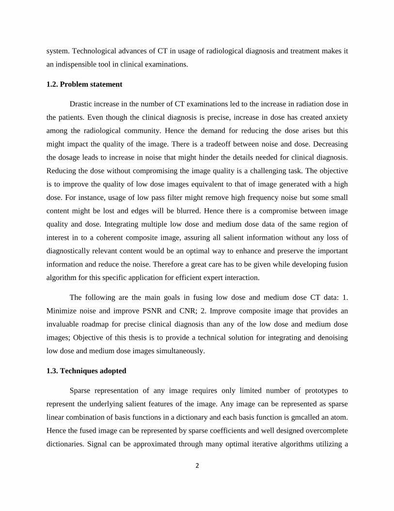
subject to (2.15)

As -norm is not smooth in nature, it has the tendency to draw best sparse solution. Thus unique

best solution from the infinitely many solutions can be drawn. Since it is mathematically

complex to draw from pool of infinite solutions, complex optimization algorithms are developed

to easily select the best unique solution.

b D

x

Figure 2.1. Depiction of sparse representation concept and the size of each matrix

2.3. Spare Approximation

1) All the sparse approximation algorithms are constructed by assuming the dictionary D to be

known.

10

The problem defined in (2.3) will have infinitely many solutions if is the span of dictionary

matrix . The solution cannot reproduce the signal b exactly since the equality constraint is

strict.

2) Considering D and b to be same as problem (2.15), applying a condition to find the solution is

given as:

subject to (2.16)

Where is the global representation error and . For this problem, the value of is flexible

since the solution is no longer required to reproduce the signal exactly and the constraint is not

too strict.

2.4. Examples of sparse representation and approximation

Sparse approximation of a randomly generated vector utilizing randomly generated overcomplete

matrix is given as:

1)

0.8147 0.6324 0.9575 0.9572 0.4218

0.9058 0.0975 0.9649 0.4854 0.9157

0.1270 0.2785 0.1576 0.8003 0.7922

0.9134 0.5469 0.9706 0.1419 0.9595

0 0.6557

1.1464 0.0357

0 0.8491

0 0.9340

0.2400

2)

0.8147 0.6324 0.9575 0.9572 0.4218

0.9058 0.0975 0.9649 0.4854 0.9157

0.1270 0.2785 0.1576 0.8003 0.7922

0.9134 0.5469 0.9706 0.1419 0.9595

0 0.6557

0 0.0357

0 0.8491

0 0.9340

0.7323

The error in second example is 0.8058 which is lower than the length of the source vector which

is 1.4229. First example has two sparse coefficients and the error is 0.4878 which is much lower

than the example with only one sparse coefficient.

11

2.5. Uncertainty

Consider the dictionary to be the concatenation of two orthogonal bases and . Simply the

dictionary is considered as the composition of identity matrix and Fourier matrix. For the

defined underdetermined system, there are many solutions that represent the signal as a

superposition of columns from the concatenated matrices that are spikes and sinusoids:

(2.17)

Optimal sparse solution represents the signal with fewer non-zero entries that is the superposition

of fewer sinusoids and spikes.

Uncertainty principle states that any function and Fourier transform of the same function cannot

be sharply localized [61].

(2.18)

Measuring the concentration in terms of standard deviation defined on and hence:

(2.19)

Signal can be represented as the linear combination of columns of identity matrix or Fourier

matrix as:

(2.20)

Where is the time-domain representation of signal b and is the frequency domain

representation of signal b. For the pair of considered orthogonal bases either or can be

sparse. Mutual coherence of the dictionary is proximity between the two orthogonal bases

which is:

(2.21)

12

If is a unit matrix and is a Fourier matrix, then mutual coherence [3] is

. Both and

cannot be sparse at the same time as is small. can also be determined as the non

diagonal entry of gram matrix as:

(2.22)

2.6. Uniqueness of sparse representation

In order to narrow the choice of well defined solution, certain constraints are applied to this

problem.

Sparsest possible solution is drawn if

(2.23)

[4] is the smallest number of linearly dependent vectors of D. Consider , the

sparse representation of the signal can be represented as:

( ) (2.24)

(2.25)

(2.26)

But the minimality nature of is contradicted. Hence the unique representation cannot

be guaranteed. But it is only upto a bounded deviation hence one can get closer to such matrices

with this scheme.

2.7. Necessity of sparse approximation

Sparse approximation algorithms are widely used in image and signal processing applications.

Obtaining the sparse approximation is not as simple as an abstract mathematical problem. It is

very challenging to store vectors containing large amount of data and computation also becomes

very tedious since Graphics Processing Units (GPUs) carry very limited amount of quickly

accessible memory. Sparse approximation techniques effectively store sparse vectors. Data can

be analyzed by the reciprocality of sparse vectors. A sparse matrix allows processes to take

13

advantage of background or zero elements and represents the underlying salient elements. Nature

of Sparsity of any matrix depends upon its structure and application.

2.8. Sparse coding algorithms

The objective of sparse problem is to obtain fewer coefficients for the given constraint

function (2.2). Obtaining exact solution for this problem is NP-hard. There are various iterative

algorithms which are used to find the objective function. During each iteration, appropriate

column vectors are chosen for obtaining the optimum global solution.

2.8.1. LASSO and Basis Pursuit

Basis Pursuit (BP) is used to substitute a complex sparse problem by an easier optimization

problem. Equation (2.2) is the formal way of defining the sparse problem. The main difficulty

with this sparse problem is the -norm. BP replaces -norm with constraint for solving the

problem with relative ease and can be defined as:

subject to (2.27)

Least Absolute Shrinkage and Selection Operator (LASSO) also known as BP de-noising

introduced in [5] replaces the sparse problem by a convex problem for efficient shrinkage and

variable selection in linear models. Derivative of the objective function is not possible due to the

constraint. This motivates the need for special optimization techniques. Grafting, which is the

stage-wise gradient descent algorithm, is developed in [6] to solve LASSO problem. However

this method is not computationally efficient. After many attempts to solve the issues faced while

solving the problem, gradient LASSO algorithm was proposed by [7] overcomes these issues.

This converges to global optimum and can efficiently handle large dimensional data set since this

algorithm does not require matrix inversion. LASSO problem can be mathematically formulated

as:

subject to (2.28)

2.8.2. Greedy Algorithms

14

Unique solution is obtained when the dictionary has , and the value of the

optimization problem is 1. Identification of columns are done when the signal is a scalar

multiple of those identified columns. Objective is to minimize the error and is represented

mathematically as:

(2.29)

Minimizing the representation error leads to:

(2.30)

Substituting in error function leads to:

(2.31)

The best solution is obtained when error is zero. Greedy pursuit iterative algorithm [8] constructs

approximation iteratively reducing the residual error. Locally optimum solution is identified at

each iteration step. Properly identifying the local optimal solutions at each step will result in a

global optimal solution.

2.8.2.1. Matching Pursuit with Time-Frequency Dictionaries

This algorithm is introduced by [9] which provides extremely flexible signal representation and

can decompose any signal in to a linear expansion of waveforms that are well localized both in

time and frequency. The property of decomposition varies with respect to the choice of time-

frequency atoms. This iterative algorithm decomposes any signal in to waveforms that well

describe the time-frequency property of the signal. Best represented signal structures that

correlate well with the given dictionary are detected and isolated by this algorithm.

Table 2.1 Pseudo algorithm of Matching Pursuit [9]

Objective: Construct an approximation for the problem P0

(P0): subject to

15

User defined input parameters: Dictionary D, Signal b and error threshold .

Initial conditions: k=0, start by setting

Intial residual (set initial solution

Initial index set

Iteration process: k=k++ (incrementing)

Sweep stage: Error computation for all . Minimizing error leads to

the optimal choice

.

Update solution stage: If the inner product between row vectors of dictionary D and

residual is and is maximum, then assign . Update the set . Set

and update the entry

Update residual stage: compute the residual .

Stopping condition: check the stopping criterion. If , global optimum solution is

obtained; Otherwise, proceed the iteration process again.

Output: is the global optimum solution obtained after iterations.

2.8.2.2. Weak Matching Pursuit algorithm

Simplified version of MP algorithm is the weak matching pursuit algorithm [9]. Greedy selection

step in weak matching pursuit algorithm is relaxed by allowing a suboptimal choice of the next

element to be added to the support set. Instead of looking for the largest inner-product value, we

select the first found that exceeds -weaker threshold. Using the Cauchy-Schuartz inequality,

(2.31)

16

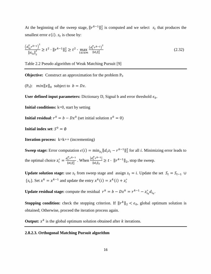
At the beginning of the sweep stage, is computed and we select that produces the

smallest error . is chose by:

(2.32)

Table 2.2 Pseudo algorithm of Weak Matching Pursuit [9]


(P0): subject to .



Initial residual (set initial solution

Initial index set



the optimal choice

. When

, stop the sweep.

Update solution stage: use from sweep stage and assign . Update the set

. Set and update the entry





2.8.2.3. Orthogonal Matching Pursuit algorithm

17

The strategy of Orthogonal Matching pursuit [8] [10] [11] makes the approximation

computationally efficient by abandoning exhaustive searches. Orthogonalization makes this

algorithm different from simple matching pursuit algorithm. Update provisional stage, which

updates the residual vector at each iteration using least square step, enhances the approximation.

The columns in dictionary D and residual should be orthogonal and already selected atoms will

not be selected in the following iterations.

Table 2.3 Pseudo algorithm of Orthogonal Matching Pursuit [8]


(P0): subject to .




Initial index set:



the optimal choice

.


residual is and is maximum, then assign . Update the set . Find the

minimizer the term such that the support is .





18

Error values in the sweep stage is represented as:

(2.33)

(2.34)

Error can be minimized if the inner product between the residual and normalized

dictionary matrix D is large.

2.8.2.4. Stage wise Orthogonal Matching Pursuit

To represent the signal sparsely faster and to solve the sparse representation optimization

problem, iterative stage wise orthogonal matching pursuit method is proposed in [12]. This

algorithm is extended from orthogonal matching pursuit algorithm. Global optimum solution is

build by adding one vector at a time in OMP algorithm, whereas many vectors are extracted at

each stage in St-OMP algorithm. Thus the number of iterations to obtain the global optimal

solution is reduced. Firstly, the residual starts out being equal to the signal. In St-OMP method,

the dot products of the signal to be approximated with the columns of dictionary are compared

and the vectors above the set threshold value are selected for the next stage. Sparse

approximation is done by applying least square method. The same process is repeated comparing

every time with the residue vector. Set threshold value should select subset of atoms with higher

correlation. Challenge lies in selecting optimum threshold value since different threshold

produces different results. Hence the results of robust St-OMP will be more sparser for optimum

threshold value.

19

Figure 2.2 Block diagram of St-OMP framework

Table 2.4. Pseudo algorithm of Stage-wise Orthogonal Matching Pursuit [12]


(P0): subject to .




Initial index set



the optimal choice

.

20


residual is and is maximum, then assign . Update the set . Find the

minimizer and the term such that the support is .





21

Chapter 3. Analytical and Adaptive

Dictionaries

Sparseland model is the basis for all the sparse image fusion algorithms described in this

thesis. All the sparse approximation algorithms are developed under the fundamental

consideration that the dictionary is known. All the sparse coding algorithms rely

heavily on costly computation with dictionary and signal on each iteration stage. Wise selection

of dictionary results in redundant representation of signal efficiently. This chapter explains the

nature of analytical and adaptive dictionaries.

3.1. Comparison of analytical and adaptive dictionary

Due to the rising need for efficient sparse representation, a variety of dictionaries have been

constructed. There are mainly two sources for dictionary development: 1) Predefined

mathematical model and 2) Realizations of training data. Analytical dictionaries such as

wavelets, Discrete Cosine Transform [13], Contourlets [14], and many more are the wise

dictionaries for fast implementation and better representation of signals in certain image

processing applications. These pre-constructed dictionaries have the ability to sparsify only the

signals having smooth boundaries. Even though these dictionaries, which are also called

22

transforms, have simple implementation, they cannot be used to sparsify many type of signals of

interest due to the analytical formulation.

By endorsing a learning point of view, learned based dictionaries overcome these limitations. On

the other hand, trained dictionaries have generating atoms as a result of learning of empirical

data instead from a theoretical model. They have the ability to sparsify any signal since they

deliver high flexibility. The implementation is complex and it’s computationally costly which do

not expose the frequency information of the signal. Hence they are limited to low dimensional

signals. In order to overcome the problems of learnt based dictionaries, these dictionaries are

handled on small patches.

3.2. Time-Frequency Dictionaries

Transformation of a signal from spatial domain to frequency domain is necessary to reduce the

observations representing the input data. Fourier transform is a widely used transform in various

image processing tasks which decomposes an image into its sine and cosine components. This

transformation exposes the frequency information of given data and divides the images based on

the frequency information thereby performing the dimensionality reduction process naturally. It

is known that Sinusoidal functions having different frequencies are orthogonal. Hence all the

signals can be effectively represented as the linear combination of a set of orthogonal sinusoidal

signals. During the earlier days, signal is represented as the combination of orthogonal basis

using Fourier Transform due to the pair-wise orthogonality nature of sinusoidal functions. This

has been widely given attention for extracting the frequency domain information of the signal.

Inner product of signal to be represented and its Fourier basis leads to the coefficients for

effective representation of the signal which is nothing but the inverse Fourier transform.

(3.1)

Signal can be represented as the combination of orthogonal waveforms by Fourier basis. To

approximate the signal, the Fourier basis creates K low frequency atoms of the dictionary. The

signals described above are smooth and have less noise.

23

3.2.1. Discrete Cosine Transform

DCT introduced in [13] is closely related to DFT but not complex. DCT decomposes the image

based on differing frequencies. Most of the energy will be accumulated in the lower frequencies

of the image. Decomposing the image based on frequency components, amount of details needed

to describe the image well can be reduced by eliminating the high frequency coefficients. Fourier

transformation works on the assumption that the signal is periodically extended which results in

discontinuous boundaries. In order to overcome this and to produce real coefficients, the signal is

assumed to be extended anti-symmetrically thereby making the boundary continuous. Due to the

efficiency of DCT, it is much preferred in practical applications.

For a signal sequence, , its number of DCT coefficients can be calculated by:

where (3.2)

And 0th

DCT coefficient is given by

(3.3)

Inverse Cosine Transform can be represented in (3.4) as

(3.4)

Two dimensional extension follows straight forwardly from single dimensional DCT, the IDCT

equation can be written as:

(3.5)

3.2.2. Overcomplete Discrete Cosine Transform

We know that every signal can be sparsely represented when the dictionary forms a basis. When

utilizing orthogonal dictionaries, salient coefficients are computed by calculating the inner

product of the signal and atoms of orthogonal dictionary. Representation coefficients are

24

computed by taking the inner product of signal and inverse of non-orthogonal dictionary and are

referred to as bi-orthogonal dictionary.

Figure 3.1. Depiction of Simple DCT Dictionary of 16 atoms and DCT Dictionary of

64 atoms

These dictionaries have limited ability to represent all the images. Due to the mathematical

computational efficiency, these orthogonal and bi-orthogonal dictionaries were predominantly

used until the development of a dictionary having more number of atoms than the signal

dimension and is called overcomplete dictionary [16].

Considering the signal length of 64, the overcomplete dictionary to be designed is presumed to

have 256 columns. In non-overcomplete case, inner product of sample and atoms shows the

representation coefficients. Transforming the sample into cosine space is done as shown in

Figure 3.2.

25

Figure 3.2. DCT dictionary with patches

Two dimensional matrix which is transformed can be represented by

1 1 1

3 15cos cos cos

16 16 16

7 21 105cos cos cos

16 16 16

In between the orthogonal bases of , non-orthogonal rows and columns are added thereby

generating an overcomplete dictionary D of size .

1 1 1

3 15cos cos cos

32 32 32

15 45 225cos cos cos

32 32 32

D

26

3.2.3. Overcomplete Haar Dictionary

The idea of using Overcomplete Haar Dictionary is first proposed in [16].

One dimensional Haar transformed matrix of size is shown below:

Overcomplete Haar transformed matrix of size is constructed by adding non

orthogonal rows in between the orthogonal bases indicated by arrows. As usual the patches are

vectorized and located at designated columns in a matrix. These columns are then normalized.

27

3.2.4. Continuous Wavelet Transform (CWT)

Wavelet transform provides flexible time frequency window to adapt to the frequencies of

different input images. This is proposed in [17] to overcome the problems of Fourier Transform.

CWT of the signal can be expressed by

(3.6)

Where defines the scale which is a positive value and represents shift which is a real number.

By shifting and scaling the basic wavelet , wavelets are generated. This basic wavelet is

well designed to be computationally efficient and easily reversible. CWT of the given

signal represents a high frequency component of the signal if the scale is larger. Undoubtedly,

window size of

will be smaller for large scale value.

3.2.5. Continuous Wavelet Transform with Discrete Wavelet Coefficients (DC-CWT)

DC-CWT overcomes the problem of intense implementation of CWT. Sampling the time scale

period parameters and values are restricted as:

and

CWT in this case is called DC-CWT and can be written as:

(3.7)

Discrete scaling and discrete wavelet functions are given by:

(3.8)

(3.9)

Where and are the FIR filters.

Convoluting and results in:

(3.10)

28

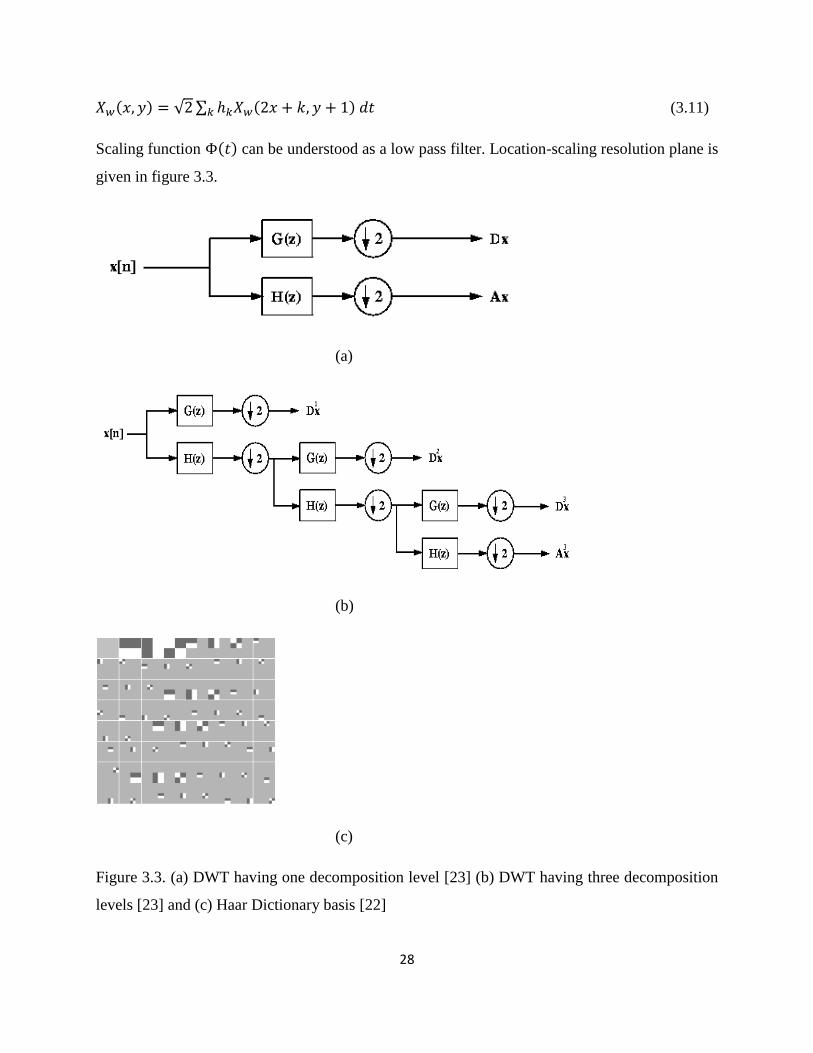
(3.11)

Scaling function can be understood as a low pass filter. Location-scaling resolution plane is

given in figure 3.3.

(a)

(b)

(c)

Figure 3.3. (a) DWT having one decomposition level [23] (b) DWT having three decomposition

levels [23] and (c) Haar Dictionary basis [22]

29

3.2.6. Discrete Wavelet Transform

Pure Discrete transforms are used in signal coding applications due to its computational

efficiency. It is the modified version of DC-CWT where both the time and time scale parameters

are discrete. Computation structure is same as DC-CWT. Simple 1D DWT having only one level

is represented in Figure 3.3. (a)

Multi-scale reconstruction of the image from transformed coefficients is done using Inverse

transform. Orthonormal filter method is used to design filters for IDWT. Shift variance property

of DWT motivates the need for complex extended DWT. DTCWT, introduced by Kingsbury

[18], was used with filters and that resulted in good shift invariance, directional selectivity and

reduced over completeness. Complex filters are applied separately to rows and columns of an

image which produces six bandpass bands at each decomposition level that are aligned at ±15,

±45 and ±75 degrees. Complex filters help in interpreting one wavelet as the real part and the

other wavelet as the imaginary part of complex-valued 2D wavelet. This complex nature

provides approximate shift invariance perpendicular to wavelet orientation. These properties can

be seen in Figure 3.4. DTCWT is vaguely represented as the union of four real orthonormal

bases of two DTCWT trees, though DTCWT is not actually the union of four orthonormal bases.

Reconstruction of the image is more accurate as the complex filters are chosen bi-orthogonal set.

Figure 3.4. Left image representing the Wavelets associated with the orientation of DTCWT and

Right image represents the Overcomplete DTCWT dictionary

30

3.3. Dictionary Learning

The prominence of dictionary learning has grown for constructing a dictionary to well

approximate a given signal. Since empirically learned dictionary can faithfully represent the

signals, they can be well used for better data fusion. Suppose a training set is generated by an

unknown model, it is not simple to identify the generating model and more importantly the

dictionary D itself. This was first addressed by Field and Olshausen in [19]. Motivated by this,

the researchers were able to develop a localized, oriented, bandpass receptive fields through

dictionary learning, which are similar to the population of simple cells in visual cortex. Later the

contributions by various other experts [16] [20] [21], resulted in the development of novel

dictionary learning algorithms. We have presented two training methods: 1) Methods of optimal

direction algorithm by Engan et al., [21] and 2) K-SVD by Aharon et al., [16].

Consider the following problem which shows that the sparse representation of signal over

an unknown dictionary . Assuming the error to be known,

subject to (3.12)

Objective of this problem is to find best representation and unknown dictionary. If the above

defined problem [24] is solved, proper representations and the generating model can be

found. This problem can also be presented by reversing roles of the penalty and constraints as:

subject to (3.13)

3.5.1 Method of Optimal Directions Algorithm

This is a frame design algorithm which aims to find true dictionary D and best representation of

the source signal. We can view the two problems (3.12) and (3.13) as nested minimization

problems. Objective of inner minimization is to obtain few non-zeros in the vector , for a

fixed dictionary D. Algorithm can be summarized as:

1) Update the dictionary in stage which is using the dictionary from

previous stage.

31

2) Using the dictionary solve instances of , one for each data set .

Solving can be done using least squares and error is evaluated using Forbenius norm:

(3.14)

(3.15)

Table 3.1. Pseudo algorithm of MOD dictionary learning strategy [21]

Objective: To find the dictionary D that sparsely represents the training vector .

Initialization:

1) Build an initial dictionary by using random entries.

2) Normalize the columns of the initially constructed dictionary.

Main Iteration: Increment by 1, then follow the steps

Sparse approximation stage: Use any efficient pursuit algorithm to find the best approximation

subject to , .

These sparsely representations for the matrix .

Dictionary update stage: Update the dictionary using, and

Stopping criterion: If change in is small enough, stop the process. Otherwise,

follow the iteration.

Output: Dictionary .

3.5.2. K-SVD Algorithm

Even though the objective of KSVD and MOD algorithms are same, difference lies in the

dictionary update stage. KSVD algorithm developed by Aharon generalizes the K-means method

for efficient dictionary learning and the atoms in the dictionary are updated sequentially. All the

32

columns in the dictionary are fixed except and . Updating the atoms can be done, along

with the coefficients that multiply them, in matrix . Modifying (3.13) by isolating the

dependency on as,

(3.16)

Error matrix is the term inside the parenthesis,

(3.17)

Optimal and to minimize the function is the best rank one approximation of . This can

be attained through Singular Value Decomposition (SVD) but this leads to a vector with more

non-zero coefficients. Minimizing the term and fixing the number of non-zero coefficients can be

achieved by selecting a subset of columns of whose entries that correspond to the original

signal from the data samples are taken and these components use the elements of in .This

may lead to the variation in existing non-zero coefficients while preserving the cardinality. To

remove the non-relevant columns by introducing a restriction matrix that multiplies from

right, is constructed with rows (number of samples in data set) and columns (number of

entries that use -atom). Restriction on the row

is defined as:

(3.18)

This is done to choose only non-zero entries. In order to achieve optimal and optimal sparse

representation , a rank one approximation via SVD is applied for the sub matrix . SVD

decomposition is applied for decomposing computation error by,

(3.19)

where is the first column of and is the first column of multiplied by .

Table 3.2. Pseudo Algorithm of KSVD Algorithm [16]

Task: To find the dictionary D that sparsely represents the training vector .

33

Initialization: Initialize

1) Build an initial dictionary by using random entries.

2) Normalize the columns of the initially constructed dictionary.

Main Iteration: Start the process by incrementing ,

Sparse approximation stage: Use any efficient pursuit algorithm to find the best approximation

subject to , .

These sparsely representations for the matrix .

Dictionary Update stage:

To minimize the optimization problem, use this stage to update both the atom and obtaining

the dictionary , for every :

1) Define the data samples that use atom ,

.

2) Compute the residual matrix and error

Obtain by restricting the pre computed error by choose only the columns

corresponding to .

Decompose the computed representation error by applying SVD decomposition

. Update the dictionary atoms by and representation by

.

Convergence criteria:

, otherwise apply another iteration.

Output: Dictionary .

34

Chapter 4. Image Fusion

Human Visual System (HVS) has an uncanny ability to visually inspect a particular scene

and mentally map the focused regions in the mind. Our human visual system can perceive

enormous focal volume even in complex challenging environment. Spatial alignment of the

object of interest, its discrete nature and its context increases the sharpness of the human

perception model. At a specified instant, human visual cortex typically perceives an object or

focal volume. Among the perceived information, a few are processed and mentally mapped but

other subset of information might be ambiguous and disregarded [30].

4.1. Introduction

Need for information fusion arose in 1950’s with a search of algorithms for integrating source

images from different sensors to obtain a composite image for identifying natural and manmade

objects with better interpretation and classification. Image fusion can be broadly defined as the

process of enhancing the perception of the scene by synergistic integration of the images of the

same scene from different sensors. The single composite image should contain all the ‘relevant’

information with increased robustness, spatial and temporal resolution for better human and

machine perception. The context of the term ‘relevant’ depends upon the application. While

35

fusing medical images, the ‘relevant’ information could be the data necessary for diagnosis.

Single image from a sensor cannot generate the accurate perception of the scene. Composite

image from the collection of images with complementary information of the same scene from

different sensors or same sensor over an extended period of time generates more description of

the scene than any of the source information. For the effective registration of source images, the

accuracy of co-alignment of sensors is very important. Determining the best framework for

obtaining the reliable composite image that enables the effective understanding of the scene in

terms of geometry and semantic interpretation is a challenging task. Benefits of fused

information include reduced uncertainty, extended spatial and temporal coverage. Recognition of

information fusion is not limited to clinical diagnosis but also extends to Geosciences, tracking

of targets in defense systems, etc.

4.2. Generic requirements of fusion algorithm

The requirements for a fusion algorithm vary with the application. General requirements of the

fusion algorithm for better representation of the scene are:

1) The fused image should preserve all the salient information while suppressing the noise

and undesired artifacts that might mislead the observer.

2) It should be highly reliable and robust to noise and misregistration.

In order to understand the challenges that we encounter when developing information fusion

algorithm, we consider two registered images of the same scene in Figure 4.1. As a result of

visual inspection, the person is clearly observed in visible image, whereas some of the details

like fence is not discernible. In contrast Infrared image of the same scene shows the fence details

clearly but the person is imperceptible.

Challenges faced for fusing these two images are:

1) Complementary information of visible and infrared images

2) There are some common objects in both the images but of extremely opposite

contrast.

3) Inputs from different sensors have different range and resolution.

36

Fusion can be simply performed by averaging or adding of source images pixel by pixel. But this

might produce undesired effects if the objects are of opposite contrast. Hence multi scale

transform fusion scheme is proposed.

(a) (b)


4.3. Preprocessing to satisfy Common Represnetation Format

Basic requirement for fusion algorithm is observation from different sensors should have

common format. Input images are compatible for fusion only when they share same

representational format. Constructing a common coordinate system is the preprocessing step for

image fusion algorithm. This conversion of source images to a common format includes:

1) Geometric and Temporal Alignment: Aligning the local spatial positions and local times

to a common coordinate system. In our thesis, we use the already registered images.

2) Feature Extraction: This process involves the extraction of characteristic features from

source images.

3) Decision Labeling: Images are transformed into multi label images by applying decision

operators.

4) Semantic Equivalence: Tranformation of input images to a same object. Images should be

semantically equivalent for feature extraction and decision labeling to be performed.

5) Radiometric Calibration: Transformation of input images to a common radiometric scale.

It’s impossible to fuse images having different radiometric calibration acquired at

different illuminations.

37

For decades, proper registering of images has been a progressive research area to make the

different source images speak a common language for further processing. The process of

aligning the multiple images of an ensemble geometrically is image registration. Basically

features of the reference image will be fixed and all the source images are aligned with respect to

common ground control point [25]. In earlier days, only the translational differences between the

source images were registered. Introduction of corner detection [28] using gradient to register the

images and introduction of segmentation to register images using optimal boundaries [26] and

approximating methods [27] facilitates the registration process to align rotational and

translational differences. Finding the acurrate transformation map that maps all the points from

fixed image to the image to be registered is the appropriate goal for effective registration.

Quality of image registration can be analysed by: 1) Transformation model: A linear model

cannot be used to register images related by non-linear transformation because that might

detoriate the registration process and 2) Precision measurement by determining the landmark

points: Locating the landmark points accurately and the use of efficient geometric transformation

model leads to a well registered image. In [29], projective transformations are used to find the

geometric relation between the images. This algorithm is constructed for the images to be

registered are capturted from different angle and field of view.

4.4. Selection methodology

Straight forward fusion techniques like arithmetic, image gradient method, etc introduce

demerits like contrast reduction in the resultant image. A good selection fusion methodology

should have noise resilience property, fused image with better contrast and should preserve all

the detailed information acclaiming high computational efficiency. Based on the mode of

operation, fusion methods are classifies as shown below [31][32]:

(1) Pixel level fusion: Pixel by pixel operation is a straight forward fusion that can be

performed in spatial domain or tranform domain. Spatial domain methods like

Principal Component Analysis (PCA), weighted average method, etc integrate pixels

using activity level measurement in a linear or non-linear fashion. In transform

domain fusion methods like Pyramid decomposition methods, Wavelet

38

Transformation method, etc. tranformed images are combined according to salience

measure. Our research uses pixel level fusion method in sparse domain.

(2) Region based methods: An image is segmented into number of regions and taking the

property of these regions into account, fusion rules are applied. Resultant fused image

is composed of focussed regions.

4.5. A brief review on area of application

This thesis applies fusion in the area of Medical Computed Tomography. The objective

of Computed Tomography [33] is to discern and visualize objects inside the human body non-

invasively. Algorithms proposed in this thesis are specifically designed for CT in clinical

applications since the issues to be considered in medical imaging and other image processing

fields are different. As the non-invasive Computed Tomography (CT) is a high dose application,

the increased radiation exposure is associated with the elevated risk of malignancy. This

increases the need for reducing the dose but low dose might lead to noise which might hinder

clinical decision making and the diagnostic process. A major area of research is devoted for

processing the low dose CT images to interpret the scene better.

4.5.1. Historical Milestones of Computed Tomography

Computed Tomography is a standard imaging modality, which has revolutionized the medical

diagnosis. CT is the first non-invasive method for acquiring cross sectional “slices” of anatomy

to understand the internal structures of the object. Beauty of this non-invasive modality cannot

be understood without the knowledge of X-rays, data processing and measurement and

instrumentation [34]. Looking back through the centuries, in 400 BC, a Greek philosopher

Democritus speculated the nature of matter as structure of invisible and indivisible particles. In

600 BC, another Greek philosopher Thales observed that amber acquires property of attracting

even light objects when rubbed with fur. The term ‘electron’ meaning amber was used since

amber acquired charge on rubbing.

The phenomenon of Faradays Electro Magnetic Induction in 1831 led Maxwell to discover that

an accelerated charge is the source of electromagnetic radiation in 1867. According to Maxwell,

electromagnetic waves which are transverse in nature can propagate through free space without

39

any material medium. Hertz in 1888 demonstrated the existence of electromagnetic waves

experimentally. In different regions of wavelength, electromagnetic waves were produced by

varying the excitation. The most important event which has revolutionized the field of imaging is

the discovery of X-rays.

In 1895, a German scientist named William Roentgen discovered when accelerated electrons

strike an anode target having high atomic weight, melting point and thermal conductivity gives

up kinetic energy and thereby produces electromagnetic rays. The physical properties of

electromagnetic waves are determined by the wavelength. Due to the unknown nature of these

rays, Roentgen called them X-rays. X-rays are shorter wavelength electromagnetic waves of

range to . These contributions are exploited by Coolidge and that led to the invention of

first rotating anode x-ray tube. First CT scanner based on a radioactive source conceived by

Hounsfield [36] and mathematical solutions to the Tomographic reconstruction problem by

Cormack [35] are some of the major breakthroughs in the development of CT. In a very short

span, CT has progressively grown to a great extent that it no longer requires optical

reconstruction techniques.

4.5.2. Working of CT

Ability of conventional X-ray radiography is limited to obtaining 2D projections for 3D

structures which results in the reduction of spatial information due to the process of averaging

[37]. Averaging produces low contrast results which are difficult to interpret even for an expert.

The need for eliminating the processing of averaging led to the development of Tomography

which has the ability to produce radiographic slices of region of interest. This is also referred to

as Tomosynthesis, if digital post processing is required. In conventional CT, X-ray tube and film

are synchronously moved in opposite directions.

The point above and below the slice are blurred and points along the center of rotation are

imaged sharply. Blurring angle determines the quality region of interest. Unlike conventional

radiography, computed tomography avoids the superimposition of blurred structures. This results

in higher contrast that enhances even the soft tissue. Four generations of CT scanners, scanners

with cone shaped X-ray beam, acquisition through slip ring technology and many other

advancements have been developed and this huge success is due to the leap in medical imaging

40

diagnosis. Clinical applications of CT have drastically increased after the subsequent growth of

helical scanning in 1980s and multi detector row technology in 1990s [43].

X-ray tube rotates perpendicularly to the length of axis of the stationary patient in a

circular orbit during data acquisition. The detector arrays are opposite to the X-ray tube that

absorbs the x-ray photons from the region of interest. The Tomogram is produced after

measuring the attenuation coefficients. Arrangement of x-ray tube and receptor array varies in

different generation scanners. Resultant image quality and dosage are interrelated.

4.5.3. Reconstruction methods

Attenuation coefficient decides the intensity of the projection image. The word image

refers to reconstructed 2D slice. The interpretation of attenuation coefficient in the object has to

be computed first. Reconstruction of internal structure of object from the measured projection

can be done through several ways. A matrix of -values for the slice is constructed. These

reconstruction algorithms [38] are customized based on projections at different angles and are

used to find the -values in each voxel of the slice perpendicular to the rotation axis. In early

days, algebraic methods were carried out for reconstructing CT images. Since they are complex

and computational intensive, computationally efficient filtered back projection methodology is

used in all the modern CT systems.

4.5.4. Computed Tomography Dose

According to the National Council on Radiation Protection & Measurements, the usage of CT in

Medical Imaging has increased more than six fold from 1980s to 2006. Approximately, around

67 million CT examinations were made in 2006 in USA alone, which was around 3 million in

1980 [39]. This rapid increase in usage of CT is due to its fast scanning speed and isotropic

spatial resolution of 0.3mm to 0.4mm which enables physicians to diagnose precisely in less time

by providing invaluable information than other imaging modalities. But the potential risk of

developing radiation induced cancer is associated with the increase of ionizing radiation

exposure. Hence reducing the radiation dose in Computed Tomography as reasonably achievable

as possible is a must to increase the benefit/risk ratio.

41

Figure 4.2. Principle of Computed Tomography [44].

Quantification of radiation dose in CT can be done using several methods such as scanner

radiation output, organ dose and effective dose for evaluating the risk of developing induced

malignancy. Volume CT dose index is a standard way of representing scanner output

level. These quantitative measures [41] do not directly represent the patient dosage rather they

represent the scanner output.

The accuracy of is doubtful for cone beam CT scanners. Organ dose is used to measure

the radiation risk association with patients’ organs according to age and sex specifications.

Energy dose is the ratio of absorbed energy to structure mass and its unit is Gray.

42

(4.1)

Since the weighting factor of different organ with respect to radiation varies, equivalent dose

of specific tissue is expressed as:

(4.2)

Considering the radio sensitivity of different organs [40], effective dose represents the weighted

sum of relative doses of individual organs and is expressed in units. Considering the tissue

weighting factor, effective dose is given by:

(4.3)

Quality of CT result is determined by the amount of radiation dose. Trade off between the image

quality and dosage level should be understood for reducing the CT dose without compromising

the image quality. Image quality is assessed by contrast-to-noise ratio (CNR) and signal to noise

ratio (SNR). Dose and SNR are be related as [40]:

(4.4)

The aspects to be considered for dose reduction are: 1) Defining and understanding the expected

image quality for each diagnostic task which allows high noise level and low dose without

compromising the clinical diagnosis and 2) To reduce image noise that might hinder important

details necessary for diagnosis. Quantum noise and electronic noise are associated with CT.

Quantum noise is determined by incident radiation and photons collected by receptor. At low

dosage values, quantum noise affects the quality of image. Fluctuation of electronic components

in CT system results in electronic noise which degrades the image quality. Optimizing the

detector and collimator in the CT system for dose performance of a CT system is very important

to reduce peripheral radiation dose. Various other factors that influence the dose are tube current,

exposition time, slice thickness and minimizing the detector size. Improving the reconstruction

algorithm and effective data processing algorithms optimally reduce noise without sacrificing the

diagnostic valuable information is important.

43

4.5.5. Computed Tomography Noise

Visual noise and increased blurring of the image impairs the visibility of anatomic structures. To

evaluate the quality of image quantitatively, signal to noise ratio is defined as the ratio of signal

level to noise level.

(4.5)

where is the mean and is the standard deviation of image. Considering two registered images

and to differentiate noise and structure, two disjoint subset of projections and

having same number of samples with and are used to

reconstruct images and . Assuming the noise in and to be uncorrelated, the

reconstructed image can be represented by [42]:

, (4.6)

(4.7)

The ideal noise free signal, is assumed to have zero noise

where is a statistical expectation operator.

Since the noise in the projections is uncorrelated, noise in corresponding reconstructed image

will also be uncorrelated. Covariance of the noises of reconstructed images is given by:

(4.8)

Local noise is estimated for each orientation to assess the difference between diagnostic detail

and noise. Reconstructed of the dataset is given by:

(4.9)

Noise can be represented as the difference between the two datasets:

(4.10)

can be represented as the linear combination of random variables with weights:

44

(4.11)

The reconstructed image include noise free signal, hence the variances can be expressed as:

(4.12)

Assuming that the noise in the projections is uncorrelated and amount of noise is approximately

equal, the relation between the standard deviation in average and input data set is given by:

(4.13)

4.6. Fusion Méthodologies

4.6.1. Image fusion using multi scale approach

Motivated by the ability of the human visual system to analyze the information at different

scales, researchers proposed the multi-scale fusion is methods. Basically, multi-scale transform

fusion, like pyramid fusion, is the transformation of synergistic combination of different levels of

information representation into an image mosaic. Firstly desired transformation is applied over

the source images. Secondly, fusion rule is applied for transformed coefficients at different levels

and each decomposition level represents different bands of image frequencies. Lastly, fused

image is recovered by applying inverse transform. Framework of pyramid based fusion is shown

in Figure 4.2.

Laplacian pyramid framework [45] supports the convolution of Laplacian decomposition map

and Gaussian pyramid of weighting map at each decomposition level. Fusion using pyramid

involves the following process:

1) The source images to be fused are decomposed to pyramid coefficients belonging to a

different frequency band which are obtained as a result of low pass filtering and sub-

sampling by a factor of 2.

45

Decision Map

Figure 4.2. Pyramid image fusion results

2) The scalar weighting map for each pixel is calculated by combining the quality

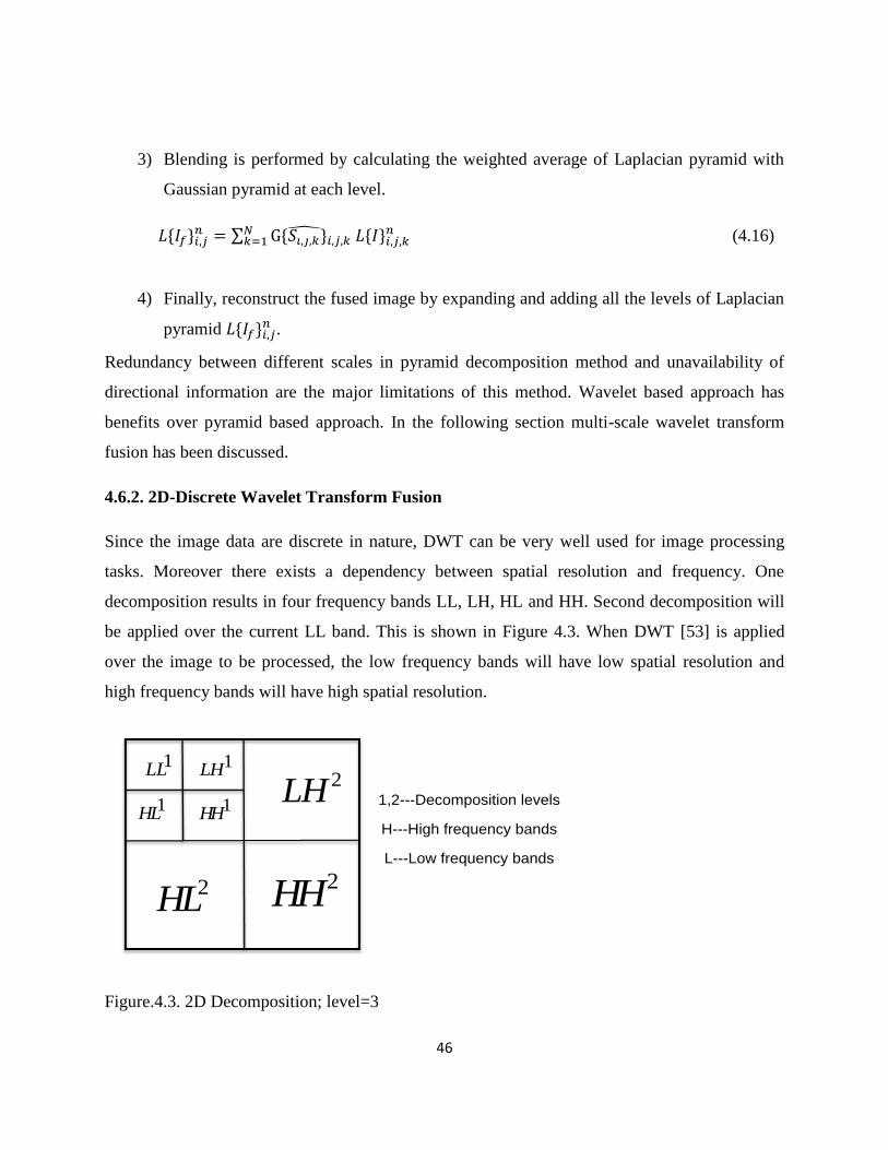
metrics contrast and the photometric measure luminance whose unit is candela per

square metre . This is represented by:

(4.14)

(4.15)

where represents the normalized weighting map, and are the weighting

components. Then the Gaussian pyramid of normalized weight map is

calculated.

46

3) Blending is performed by calculating the weighted average of Laplacian pyramid with

Gaussian pyramid at each level.

(4.16)

4) Finally, reconstruct the fused image by expanding and adding all the levels of Laplacian

pyramid .

Redundancy between different scales in pyramid decomposition method and unavailability of

directional information are the major limitations of this method. Wavelet based approach has

benefits over pyramid based approach. In the following section multi-scale wavelet transform

fusion has been discussed.

4.6.2. 2D-Discrete Wavelet Transform Fusion

Since the image data are discrete in nature, DWT can be very well used for image processing

tasks. Moreover there exists a dependency between spatial resolution and frequency. One

decomposition results in four frequency bands LL, LH, HL and HH. Second decomposition will

be applied over the current LL band. This is shown in Figure 4.3. When DWT [53] is applied

over the image to be processed, the low frequency bands will have low spatial resolution and

high frequency bands will have high spatial resolution.

2HH2HL

2LH1HH

1HL

1LH1LL

1,2---Decomposition levels

H---High frequency bands

L---Low frequency bands

Figure.4.3. 2D Decomposition; level=3

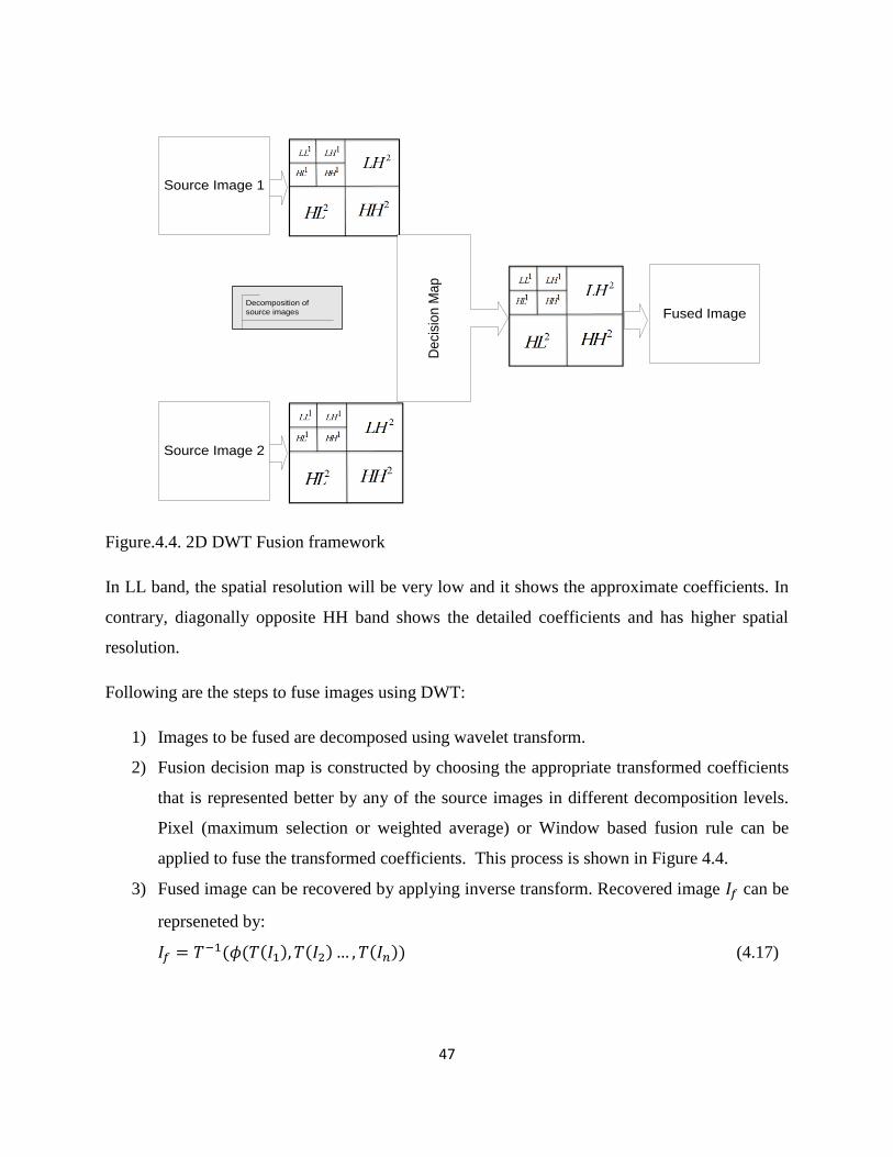
47

De

cisi

on

Ma

p

Source Image 1

Source Image 2

Fused ImageDecomposition of

source images

Figure.4.4. 2D DWT Fusion framework

In LL band, the spatial resolution will be very low and it shows the approximate coefficients. In

contrary, diagonally opposite HH band shows the detailed coefficients and has higher spatial

resolution.

Following are the steps to fuse images using DWT:

1) Images to be fused are decomposed using wavelet transform.

2) Fusion decision map is constructed by choosing the appropriate transformed coefficients

that is represented better by any of the source images in different decomposition levels.

Pixel (maximum selection or weighted average) or Window based fusion rule can be

applied to fuse the transformed coefficients. This process is shown in Figure 4.4.

3) Fused image can be recovered by applying inverse transform. Recovered image can be

reprseneted by:

(4.17)

48

Work flow of DTCWT Fusion [51] is presented in Figure 4.5. First, the Source images to be

fused are decomposed into detailed and approximate coefficients using DTCWT. Fusion rule is

applied to form decision map. Fused image is recovered by applying inverse transform.

(4.18)

Decision Map

1I2I

1( )DTCWT I 2( )DTCWT I

IDTCWT

Figure.4.5. 2D DTCWT Fusion framework

4.6.3. Principal Component Analysis based fusion

49

This unsupervised dimension reduction technique is based on the idea of projecting the high

dimensional information into a low dimensional sub-space. Specifically, this technique is carried

out by constructing the covariance matrix from the input images [47] [46].

To understand this best known linear sub-space transformation technique, we consider an image

having rows and columns as a one dimensional vector . Finding the low dimensional

subspace in which the input image resides from the dimensional space is the basic idea of

this statistical technique. If is a array that represents a set of

orthonormal basis functions, the transformation into a single dimensional vector of reduced

length can be represented as follows:

(4.19)

where is a column vector and has the length . Approximation of can be

reconstructed from by applying inverse transform as:

(4.20)

Error obtained from recovered vector and the input vector should be minimal.

To adequately represent the source images as the linear combination of orthogonal basis, we seek

the orthonormal vectors with . For a given training set of images

represented by one dimensional vectors, directions are selected along the training vectors

having largest variances. The dimension is reduced to by discarding the directions having

minimal variance.

Lower dimensional representation enhances the generalization and the visualization. Hence it

provides better understanding of essentialities in the information. Manipulations performed in

low dimensional space is computationally efficient than manipulating high dimensional data

since the latter requires more memory and consumes more time.

Considering the spatially and temporally aligned source images to be fused and of size

, the orthonormal vectors are . Columns vectors of source images can

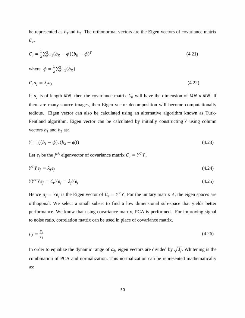
50

be represented as and . The orthonormal vectors are the Eigen vectors of covariance matrix

.

(4.21)

where

(4.22)

If is of length , then the covariance matrix will have the dimension of . If

there are many source images, then Eigen vector decomposition will become computationally

tedious. Eigen vector can also be calculated using an alternative algorithm known as Turk-

Pentland algorithm. Eigen vector can be calculated by initially constructing using column

vectors and as:

(4.23)

Let be the eigenvector of covariance matrix ,

(4.24)

(4.25)

Hence is the Eigen vector of . For the unitary matrix , the eigen spaces are

orthogonal. We select a small subset to find a low dimensional sub-space that yields better

performance. We know that using covariance matrix, PCA is performed. For improving signal

to noise ratio, correlation matrix can be used in place of covariance matrix.

(4.26)

In order to equalize the dynamic range of , eigen vectors are divided by . Whitening is the

combination of PCA and normalization. This normalization can be represented mathematically

as:

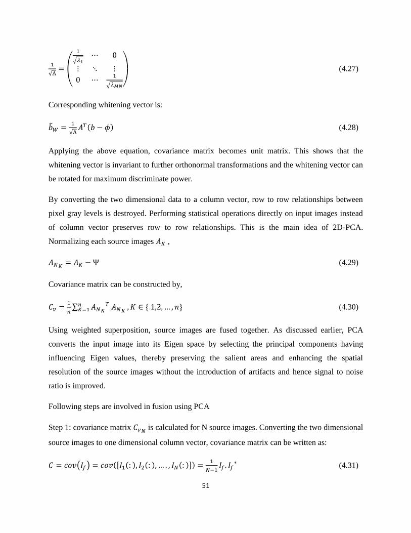
51

(4.27)

Corresponding whitening vector is:

(4.28)

Applying the above equation, covariance matrix becomes unit matrix. This shows that the

whitening vector is invariant to further orthonormal transformations and the whitening vector can

be rotated for maximum discriminate power.

By converting the two dimensional data to a column vector, row to row relationships between

pixel gray levels is destroyed. Performing statistical operations directly on input images instead

of column vector preserves row to row relationships. This is the main idea of 2D-PCA.

Normalizing each source images ,

(4.29)

Covariance matrix can be constructed by,

(4.30)

Using weighted superposition, source images are fused together. As discussed earlier, PCA

converts the input image into its Eigen space by selecting the principal components having

influencing Eigen values, thereby preserving the salient areas and enhancing the spatial

resolution of the source images without the introduction of artifacts and hence signal to noise

ratio is improved.

Following steps are involved in fusion using PCA

Step 1: covariance matrix is calculated for N source images. Converting the two dimensional

source images to one dimensional column vector, covariance matrix can be written as:

(4.31)

52

where is the fused image.

Step 2: Eigen space of the covariance matrix can be calculated by:

(4.32)

where is the eigenvector and is the influencing Eigen value

Step 3: Eigen vector can be normalized by:

(4.33)

Step 4: Normalized Eigen vector of maximum Eigen value is selected. Final fused image is

reconstructed by considering these Eigen vectors as weightings.

Figure.4.6. PCA Fusion framework

53

4.7. Image Quality Measurement

Assessing the performance of a fusion result is done based on quantitative and qualitative

measures. Qualitative analysis is the measure of observers’ experience and can be done by

quantifying the subjective evaluation done by experts. Measuring the quality of image

mathematically without any human observer is image quality metric. There are mainly two

different ways of quantitatively measuring the quality of fused image based on spatial and

spectral similarity: 1) Non-reference method which states the quality of the fused image without

requiring any reference. This is very challenging due to the lack of ground truth. 2) Reference

method which requires both reference and composite image for IQ metric evaluation. Brief

reviews on some of the metrics which are used in thesis are presented as follows:

Entropy: It measures the amount of details in the image; the high entropy indicates high details.

Since the first order entropy doesn’t consider the spatial correlation, therefore we employed the

second order entropy as quality evaluation which will enable us to measure the transition

between gray levels. The second order entropy is based on the co-occurrence matrix and its

probability as given bellow [45][54],

(4.34)

where

Absolute mean brightness error (AMBE) [45]: It measures the shift in mean intensity of the

fused image from mean intensity of the original image and it is given as [54],

(4.35)

Mutual information [54]:

To find the mutual information of registered image I1 and reference image Ir,

1

1

1

,

1 , 2

( , )( , ) ( , ) log

( ), ( )

r

r

r

I I

r I I

I I

p a bMI I I p a b

p a p b

(4.36)

54

where 1 , ( , )rI Ip a b

is the joint probability a pixel (x, y) in I1 has a gray-level a and the same pixel

in B has a gray level b.

Normalized mutual information may vary if the number of pixels which are common

to the source images changes. Even a small variation may lead to inaccuracies in this spatial

alignment. So normalized mutual information can be used:

1 1

1 1

1 1

1 1

1

2 2

1

2 2

11

, 2 ,

1

2

( , )

( ) log ( ) ( ) log ( )

( , )

min( ( ) log ( ) , ( ) log ( ) )( , )

( , )

( , ) log ( , )

( , )

( ) log ( )

r r

r r

r r

r

I I I I

r

I I I I

rr

I I I I

r

I I

MI I I

p a p a dxdy p b p b dxdy

MI I I

p a p a dxdy p b p b dxdyNMI I I

MI I I

p a b p a b dxdy

MI I I

p a p a dxdy

2. ( ) log ( )r rI Ip b p b dxdy

(4.37)

PSNR [54]: It is Peak Signal to Noise Ration which is used to measure the reconstruction quality

of fused image. PSNR of the fused image If is calculated using the standard formula:

2

10( ) 10logf

MPSNR I

MSE

(4.39)

where M is the maximum possible pixel value of the image and MSE is the Mean Square error.

While the SNR and RMSE are given as follows, where r(x,y) is the reference image and t(x,y) is

the fused image .

(4.38)

(4.40)

55

SSIM [55]: It is the Structure Similarity Index which provides structural information of objects

in the image. This measure is based on similarity of contrast of local patch , structure of

local patch and luminance of local patch . PSNR estimate perceived errors where as

SSIM assumes image degradation as the perceived change in structural information. Structural

information considers the spatially close pixels having strong inter-dependencies that carry the

salient details. Range of SSIM is between -1 and 1, and value 1 occurs only for identical data set.

Contrast to Noise Ratio (CNR)

There is a tradeoff between radiation quality and contrast and effect or influence of this can be

described using Contrast to Noise Ratio (CNR) [56]. CNR has certain properties which are given

below:

1) Relates to contrast difference between larger object and background of the image.

2) Relates to exposure factors.

3) Doesn’t incorporate any information about resolution.

56

Chapter 5. Proposed Methodologies

5.1. Image Fusion Using Simultaneous Controlled St-OMP

The goal of integrating the source images using sparse representation method is to enhance the

important details without the introduction of distortion. Signal can effectively be represented by

sparse representation as the linear combination of effective sparse model and well designed

dictionary. Salient features of the images can be represented with least number of coefficients

using sparse representation which is effective than traditional multi transform methods because

of the nature of sparsity and overcompleteness of dictionary. Sparsity results in many zero

coefficients thereby leading to the improvement of computational efficiency. It is not necessary

for the atoms to be orthogonal in overcomplete dictionary and number of atoms are more than

number of image pixels. We utilize Modified Cosine Transform Dictionary generated by cosine

basis functions incorporated with shift variations. We use sparse approximation and utilize

effective dictionaries to fuse low dose and medium dose CT images. The process of image fusion

using sparse representation contains two stages: Signal approximation stage and fusion stage. In

signal approximation stage, all the patches of the source images are transformed into linear

combination of atoms of, MDCT dictionary tailoring matching pursuit methodology specifically

designed for fusion application. Generally, the approximation solution is achieved by matching

pursuit algorithms through an iterative process. Locally optimum solution is obtained in each

iteration when residual vector closely resemble the vector to be approximated and global

57

optimum solution is obtained after the sequence of locally optimum solutions. Due to the

computational efficiency of OMP over BP, it is used to solve the optimization problem in

applications. In fusion stage, global approximated solution of source images are integrated by

applying absolute maximum fusion rule.

Inspired by [52], we are proposing a simultaneous approximation method which adopts CSt-

OMP for representing the several source images as linear combination of elementary signals at

once. St-OMP discussed in previous chapter that uses many atoms each stage solves the

optimization problem in less iteration. St-OMP uses threshold value in the aim of selecting

highest matching atoms from the well designed dictionary. So the approximation depends upon

the threshold value and every atom above the threshold value contributes to reconstruct the

signal. So lower threshold might allow more non-zero entries at each stage. In contrast, high

threshold allows only few non-zero entries each stage to reconstruct the signal. But this takes

more iteration to find the approximate solution due to the dependency on threshold value and it is

computationally intense due to the calculation of pseudo inverse at each stage. In order to

overcome this, CSt-OMP is proposed to approximate a single input signal at a time.

We propose Simultaneous CSt-OMP that adopts a different atom selection strategy that solves

the optimization problem more efficiently and in less time. Considering a matrix of size

whose columns are source images, Simultaneous CSt-OMP solves the following

optimization problem:

subject to (5.1)

where is the coefficient matrix having non zero coefficients.

58

Figure 5.1. Framework of proposed Simultaneous Controlled St-OMP fusion

In this algorithm, number of atoms to be added at each stage is pre-declared thereby reducing the

dependency on preset threshold value. Framework of the proposed method is shown in figure

5.1. The residual matrix starts out to be the corresponding training signals itself. The objective of

each iteration is to minimize the optimal simultaneous representation error at each stage.

Hard thresholding selects the matching atoms when the inner product of row vectors of

dictionary and residual is maximum and these selected atoms are stored in a local dictionary

to be updated. In the seletion strategy, largest matching atom is selected. Covariance of

largest matching atom with is computed and the least correlated atom is chosen as the

second representative since it contributes more on signal reconstruction. The process should be

repeated unless the reconstruct error is optimally minimum. Due to the less dependency on

threshold value, at the same time using two atoms in each stage and approximating

simultaneously makes this algorithm efficient than SOMP algorithm.

59

Table 5.1. Pseudo algorithm of proposed Simultaneous Controlled St-OMP fusion


(P0): subject to and fuse the approximated coefficients

User defined input parameters: Dictionary D, Signal matrix for source images and error

threshold .

Sparse coding stage


Initialize residual matrix (set initial solution

Initial index set


Sweep stage: Calculate the correlation of residual and dictionary D.

Hard Thresholding stage: and store the atoms in local dictionary .

Update solution stage: If the inner product between row vectors of local dictionary

and residual is and is maximum, it is the most relevant first atom. Calculate the covariance

between maximum matching and , then select the least representative as second atom.

Update the solution: Obtain the approximation , by

the solution to

Stopping condition: check the stopping criterion. If , global simultaneous optimum

solution is obtained; Otherwise, proceed the iteration process again.

Approximation stage output: is the global optimum solution obtained after iterations.

Fusion stage

60

Output: Reconstructed final fused image .

We assume the source images to be spatially aligned. If the source images are not registered,

proper registration algorithms should be used to align the image spatially and temporally in order

to avoid geometric distortion. Consider geometrically registered source images. The fusion

process is given below:

1) Source image is divided into possible patches using sliding window

technique and then all the patches are transformed into -dimensional column vector.

2) Using CSt-OMP, find the sparse approximation of corresponding vectors.

3) Fusion rule to be applied

Choosing the appropriate fusion rule determines the quality of final fused image. There

are two important concerns to be addressed for fusion using pixel level algorithms 1)

Activity level measurement identifies the salient coefficients of the source images. 2)

Coefficient combination uses the salient coefficients from the source images in to the

fused image. Weighted average fusion scheme smoothens the salient information. Thus

maximum absolute fusion rule is applied to preserve the salient information.

(5.2)

(5.3)

4) Fused vector is calculated by:

(5.4)

5) Final fused image is recovered from vector by reshaping this to block size of

. Each pixel position of the fused image is the summation of several block

values. Final image is obtained by dividing each pixel of the final image by number of

summations occurred at that pixel.

6) The overcompleteness nature of dictionary and the sliding window technique makes this

algorithm shift invariant.

61

5.2. Medical Image Fusion Based on Joint Sparse Method

Image fusion using sparse representation methodology guarantees robustness which can extract

the underlying information from source images effectively. As we have seen in previous

chapters, sparse representation techniques are used to represent signals with the fewest number

of non-zero coefficients.

For a signal , sparse representation assumes the representation of the signal as a linear

combination of given atoms from the overcomplete dictionary where ( ).

Overcomplete dictionary has the capability to sparsify the signal efficiently since number of

atoms exceeds number image pixels. Every signal can be represented as , where

is the sparse vector that contain few salient entries. Since dictionary has more number of

columns than rows, is an under-determined system and there can be infinite solutions.

Finding the approximate solution for the signal is not easy due to the strict equality constraint.

Hence, the following optimization problem is solved to find the best approximation:

subject to (5.5)

where represents the number of non zero coefficients which can be positive or negative in

and is the representation error. Since the above defined optimization problem is NP-hard,

greedy algorithms are used to solve due to the computational efficiency and less intense nature.

Non-zero sparse coefficients of the source images are considered to be the salient features for

fusion. In this section the problem of fusion and denoising low dose CT images can be

simultaneously addressed. Low dose and medium dose CT images of the same region of interest

possess their own characteristics and also share common information. Sparse coefficient vectors

are estimated for representing the ensemble of source images to be fused using the matching

pursuit methodology. Proposed algorithm effectively extracts the common and complementary

information and integrates effectively.

This thesis proposes a new algorithm inspired by joint sparse representation model for

compressed sensing [62], which employs different rules to extract common and innovative

62

sparse components from the source images. Inspired by [62] [48] and [60], a novel image fusion

algorithm is proposed which integrates the source vectors in sparse domain using Principal

Component Analysis.

Low dose and medium dose images of the same region of interest to be fused form an ensemble.

Sparse theory states that any signal can be sparsely represented. In the same way, the ensemble

of signals are represented by where will also have joint sparse nature. That

means all the data in an ensemble will have a common sparse component and each image will

have innovative sparse components. Assuming the sparse basis is known where is

approximately represented. For the signal , let the measurement matrix be of size .

And the measurement matrix will have different entries for different .

Joint sparse model I: Sparse common component many innovative components

In this model, all the source signals will have common components and each signal will have an

innovative component and this can be represented as:

, (5.6)

where and . This means the is the common component of and

in basis . Whereas are the unique proportions of ensemble having

in the same basis . We use joint sparse model I for our experiment.

Joint sparse model II: Common sparse model

In this model, all the signals which are taken over an extended period of time are constructed

from same basis but having different coefficients :

, (5.7)

Thus all the signals can be represented sparsely with non-zero coefficients using different

coefficient in the same basis having elements.

For a signal , there is a common component

and innovative components

. Signal can be represented as:

63

(5.8)

Where is the overcomplete dictionary and is the noise component.

Innovative components might contain noise. The above equation can be sparsely represented by:

1

1

1

2

0

0 0

0n

C

I

n

I n

D D nB

D n

BD D n

(5.9)

This can be generally written as:

(5.10)

if

1

1

0

0 0, ,

0n

C

I

n

I

D DB

DB D

BD D

and

1

2

n

n

nn

n

(5.11)

Extracting the among the source images is the most challenging task.

Sparse vector can be calculated using any of the sparse approximation techniques for solving the

following optimization problem,

subject to

(5.12)

In our proposed method, we apply simultaneous controlled stage wise orthogonal matching

pursuit proposed in the previous section to solve it. Selection of efficient dictionary plays an

important role in extracting the salient features from the source images. As we know the

limitations of fixed dictionaries, we use dictionary learning technique to learn the basis vectors

that are capable of well representing the signal.

64

The source images are traversed from left top to right bottom using sliding window technique

and divide the image into number of patches. These patches are then converted

lexiographically into column vectors for each image . As discussed all the source

images are constructed using the same subset of atoms in the dictionary. Sparse coefficients are

considered as image features where the coefficient of each patch is calculated separately by

solving the optimization problem under the overcomplete dictionary . The signal in the

ensemble can be represented as:

(5.13)

Where and denotes the sparse coefficients of common and innovative information and

JSM can be represented as:

(5.14)

where is the ensemble assuming the signals are noiseless and

, Dictionary

and

But ensemble of low dose and medium dose images can be represented as:

(5.15)

where is the noise. can be obtained by solving the optimization problem using the

Simulataneous CSt-OMP method with appropriate error tolerance. The detailed steps of the

algorithm are summarized:

1) We assume the source images have common representation format. All the

images to be integrated are divided into patches using sliding window technique

and are lexicographically transformed to -dimensional column vectors. Each source

image will have patches.

65

2) Mean values of patches of the source images is

subrtracted from the patches and can be represented as:

(5.16)

where is the joint representation of a common component

and two innovative

components

and can be calculated by solving the optimization problem.

3) Appropriate fusion rules are applied to integrate the sparse vectors. Fused innovative

sparse vector is obtained by integrating innovative sparse vectors using PCA rule.

Using PCA, orthogonal directions enhancing the variance of the innovative sparse vectors

is obtained. Unlike other fusion rules in sparse domain, PCA preserves salient features

while eliminating the artifacts since innovative components might have noise. PCA

converts sparse vector into its Eigen space which is done by selecting principal

component having influencing Eigen values. Covariance matrix of sparse vectors is

calculated as:

(5.17)

Then the Eigen space of the covariance matrix is calculated by:

(5.18)

where is the Eigen vector and

is the Eigen value. Normalized Eigen vector of

maximum Eigen value is chosen as the weightings of the images to be fused.

(5.19)

Innovative fused vector is obtained by:

(5.20)

4) Fused innovative vector and sparse vector of common component are fused using

“choose-max” rule since the common components are noiseless, that is the vector with

66

maximum norm is considered as the salient feature. Weighted average fusion rule is

used to fuse the mean values.

(5.21)

JSR MODEL

We

igh

ted

Ave

rag

e F

usio

n

1I

2I

NI

Reconstructed

fused image

from fused vector

1

ib

2

ib

N

ib

'

1b

'

2b

'

Nb

1m

2m

Nm

C

1I

NI

2I

SCSt-OMP

Figure 5.2. Framework of Joint Sparse PCA fusion methodology

Weighted average fusion of mean values can be done by:

(5.22)

67

where the weighting parameter

5) Final fused vector is calculated by combining with the overcomplete dictionary:

(5.23)

Lastly, is reshaped into a block of size . All the blocks are appropriately placed

in the specific location of the fused image. Many block values represent single pixel value

due to the usage of sliding window technique and hence final fused image is obtained by

average processing at each pixel location.

Table 5.2. Pseudo algorithm of Joint Sparse PCA fusion method

Objective: To integrate the source images

User defined input parameters: Dictionary D, source images mage and error threshold

.


Initialize residual matrix: (set initial solution

Initial index set:


Sparse coding stage:

-Common and innovative vectors through JSR

-Patches of the original images are subtracted from the mean of patches

-Stopping condition: check the stopping criterion. If , global simultaneous optimum


68

Fusion stage:

-PCA fusion to integrate innovative vectors

-weighted average rule to fuse and common component

-weighted average of mean values

Output: Reconstructed final fused image .

5.3. Simultaneous medical image fusion and denoising using focused region in sparse

domain

To the best of our knowledge only the contributed methods in this thesis are used to fuse low

dose and medium dose images and denoise them simultaneously. It is necessary to know that

most of the fusion algorithms are developed based on the assumption that the images are noise

free. Such algorithms are effective for noise free images and presence of noise might

compromise the quality of fusion. Since the proposed hybrid Sparse PCA method seems to show

promising results, a novel image fusion is proposed which uses an initial fused image from the

previous method. Then in sparse domain, pixels of fused image similar to the pixels of the

original image are determined and considerably focused region map is obtained. Final fused

image is obtained after simultaneous dictionary learning, fusion and denoising in sparse domain.

This algorithm is designed for both noisy and noise free source images.

5.3.1 Dictionary learning and acquisition of initial fused image

First step starts out to be dividing the source images in to using sliding window

technique and lexicographically ordered as -dimensional column vectors . From the previous

section we know that, an ensemble of intercorrelated images has a common component and

multiple innovative components. Initial fused vector

is obtained by Joint Sparse PCA method

that employs different fusion rules for integrating common, innovative sparse components and

mean of patches. Dictionary learnt from high dose patches are used for representing the signal.

Integrated image is obtained by:

69

(5.24)

where

is the fused vector of common and innovative sparse vectors and

is the fusion of

mean of patches and dictionary is trained using high dose patches.

Dictionary learning method is used for joint sparse fusion method. Proposed method uses a

dictionary learning method specifically for joint sparse model. Let us assume an ensemble ,

containing low dose and medium dose images.

Mathematical definition of objective function can be written as:

subject to (5.25)

where this function denotes sparsity, denotes the number of non zero coefficients.

Optimization problem subject to certain amount of error tolerance is give by:

subject to (5.26)

Where represenets the dictionary that governs the optimality of sparse representation. Firstly,

joint sparse coding is done and is obtained through proposed simultaneous controlled OMP by

fixing the dictionary and the general equation can be represented as:

1

1

0

0 0

0N

CC I

IC

N

C I I

D Ds

Dn

sD D

(5.27)

Then the dictionary is updated keeping fixed by solving the problem given below:

(5.28)

This can be extensively written as

70

1

1

...min [ .... ] [ ]

...C IN

C C

N C ID D

I I

S S D D

(5.29)

Optimum is obtained by setting the gradient function to zero:

(5.30)

For

and

Then we yield,

(5.31)

When rank of the matrix H is not then according to Land weber [61],

(5.32)

where noise intensity . Iterative joint sparse coding stage change and hence

spectral norm has to be calculated again. A good initial point hasten the computation since

Hermitian matrix’s spectral norm is known for its enhanced Eigen value [61].

If SVD of is , dictionary is initially updated by

(5.33)

Due to the diagonal dominance theory [61], optimum of the equation (5.32) is obtained. We

normalize the atoms in the dictionary so that and if , the corresponding

coefficient is scaled but when , any non-zero column of is substituted after the

normalization of atoms.

71

5.3.2. Detection of focused region and fusion scheme

Source vectors and initial fused vector are compared and similar points are determined. Using

certain quantitative measures like RMSE and correlation, proper focused vector

is

designed. Source image vectors, focused vector and initial fused vector are jointly represented as

common and innovative components using a trained dictionary after subtracting from the mean

of the corresponding patches.

= (5.34)

where is obtained by applying PCA fusion for integrating innovative components

. (5.35)

Final fused vector is obtained by

(5.36)

where

is the composite vector of common and complementary components and is

obtained by applying weighted average rule to fuse the mean of patches of JSR components.

Finally, the final image is constructed by positioning the blocks in designated location and

averaging each pixel location.

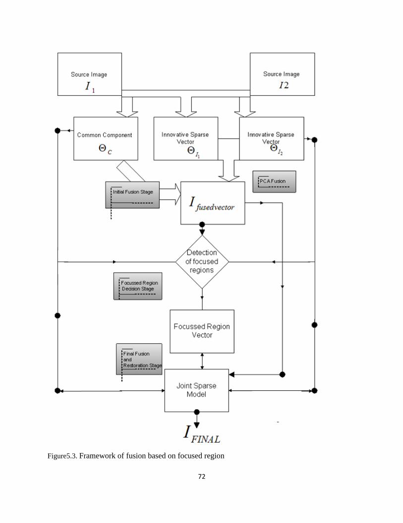
72

Figure5.3. Framework of fusion based on focused region

73

Table 5.3. Pseudo algorithm of fusion based on focussed region

Objective: To integrate the source images

User defined input parameters: Dictionary D, source images and error threshold .


Intialize residual matrix (set initial solution

Initial index set


Initial fused image stage:

objective function is solved by 1

1

...min [ .... ] [ ]

...C IN

C C

N C ID D

I I

S S D D

1, ,.....,

N

C

I I obtained at the end of all iterations.

Initial fused image is obtained by 1

( , ,....., )N

C

initial I II

Focused region detection stage: Focused vector is selected by comparing

1, , ,...,

N

C

initial I I

Final fusion stage: Final fused vector is 1( , , ,....., )final Initial focussed NJSR

Stopping condition: check the stopping criterion. If , global simultaneous optimum


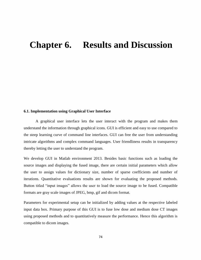
74

Chapter 6. Results and Discussion

6.1. Implementation using Graphical User Interface

A graphical user interface lets the user interact with the program and makes them

understand the information through graphical icons. GUI is efficient and easy to use compared to

the steep learning curve of command line interfaces. GUI can free the user from understanding

intricate algorithms and complex command languages. User friendliness results in transparency

thereby letting the user to understand the program.

We develop GUI in Matlab environment 2013. Besides basic functions such as loading the

source images and displaying the fused image, there are certain initial parameters which allow

the user to assign values for dictionary size, number of sparse coefficients and number of

iterations. Quantitative evaluations results are shown for evaluating the proposed methods.

Button titled “input images” allows the user to load the source image to be fused. Compatible

formats are gray scale images of JPEG, bmp, gif and dicom format.

Parameters for experimental setup can be initialized by adding values at the respective labeled

input data box. Primary purpose of this GUI is to fuse low dose and medium dose CT images

using proposed methods and to quantitatively measure the performance. Hence this algorithm is

compatible to dicom images.

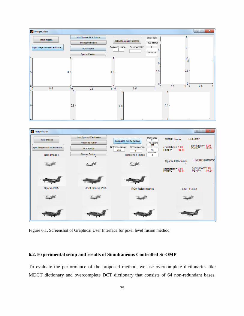
75

Figure 6.1. Screenshot of Graphical User Interface for pixel level fusion method

6.2. Experimental setup and results of Simultaneous Controlled St-OMP

To evaluate the performance of the proposed method, we use overcomplete dictionaries like

MDCT dictionary and overcomplete DCT dictionary that consists of 64 non-redundant bases.

76

Overcomplete dictionaries which can also contain non-orthogonal atoms, overcomes the

limitations of fixed dictionary. MDCT dictionary used in our proposed method is created with 6

shifts in the first part, 4 in the middle and 2 in the last and is shown in Figure 6.6 (b).

Overcomplete DCT is constructed using 29 frequency divisions from to without any phase.

Constructed dictionaries contain 841 atoms and are used to approximately represent the images

in sparse domain using the conventional OMP fusion method and the proposed method.

Two parameters decide the efficiency of sparse coding stage: 1) Selection of appropriate size of

sliding window and 2) Global representation error. We know that dictionary size is large for

larger sliding window size and computational efficiency becomes lower. Decreasing the size of

sliding window makes the sparse coding algorithm to perform faster. But with smaller sliding

window, the patches might miss some of the salient information. After trial and error,

appropriate sliding window size of is chosen so that the important features of the low dose

images are not being missed. And the patches are chosen without any overlapping. We set the

stopping criterion as global representation error . Threshold value used in the proposed

method is 0.6 and 16 atoms are used to represent the images sparsely.

Performance of the proposed algorithm is compared with well known methods like OMP fusion

and SOMP fusion methods. SCST-OMP is the extended version of SOMP fusion method with

the following differences: 1) Fusion algorithm in [52] is developed using Overcomplete DCT

dictionary of size which is shown in Figure 6.6.(a). 2) Core idea of SOMP is to extract

one atom in each stage.

Proposed algorithms are developed in MATLAB GUI 2013 environment for measuring the

realistic computational time. Experiment is performed on natural images and some of the

provided CT phantoms with the assumption that they all have common representation format.

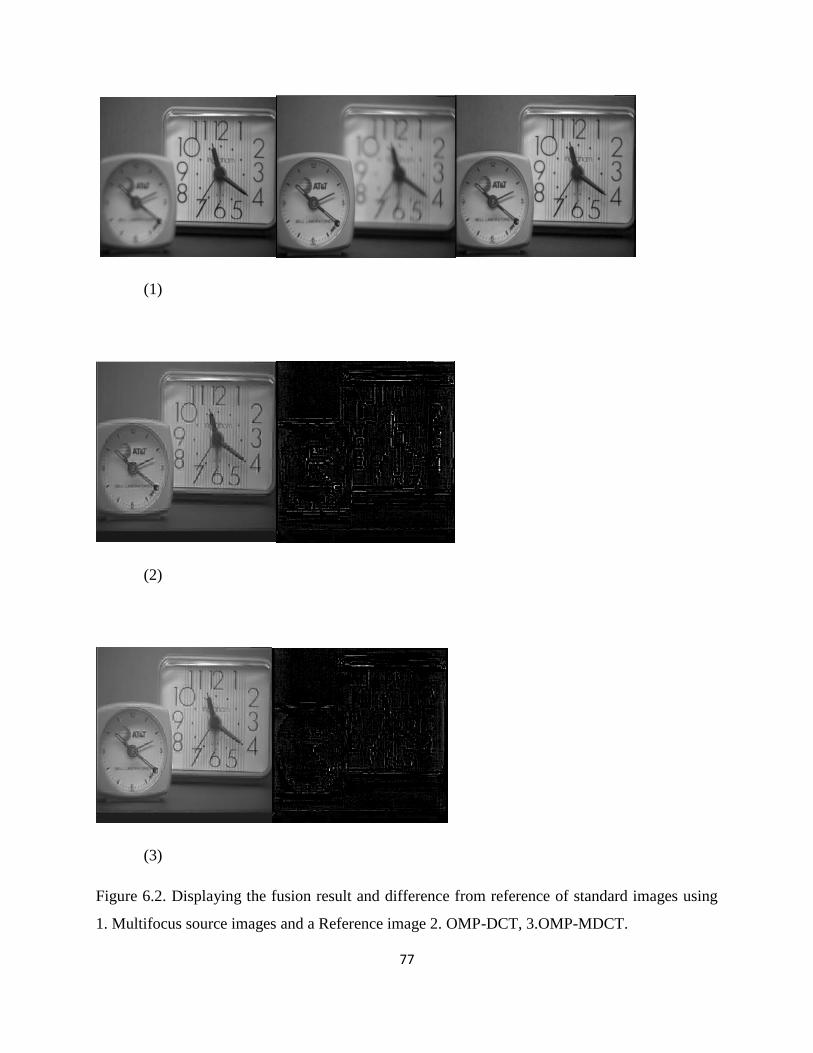
77

(1)

(2)

(3)


1. Multifocus source images and a Reference image 2. OMP-DCT, 3.OMP-MDCT.

78

(4)

(5)

(6)


4. SOMP-MDCT, 5. SCStOMP-DCT and 6. SCStOMP- MDCT.

79

In order to validate the performance, we investigate the performance of the proposed method by

performing the experiment on standard images and CT images. All the source images used were

geometrically registered. Firstly the proposed method is experimented on multi focus clock

images. First row of the Figure 6.1 presents the source images having two clocks to be fused and

a reference image. First source image is captured by focusing the big clock and second source

image is captured by focusing the small clock. Visually, the fusion result of OMP-DCT and

OMP-MDCT seem to have low spatial resolution and the difference is more obvious. We can see

that OMP-DCT fusion result contains artifacts. Results using simultaneous fusion methodology

have clear details and better spatial resolution than OMP fusion methods. Proposed fusion

method utilized MDCT dictionary contain clear clocks.

Table 6.1. Performance evaluation of proposed method for standard images quantitatively

Source Images Methodology PSNR

(db)

SSIM Correlation MI

Clock

(Multifocus)

OMP-DCT 28.8290 3.2442 0.8966 0.9966 0.5011

OMP-MDCT 29.9021 3.1751 0.8999 0.9973 0.5147

SOMP-MDCT 31.2682 2.9144 0.9666 0.9980 0.5142

SCSt-OMP DCT 31.5374 2.9239 0.9667 0.9981 0.5164

SCSt-OMP MDCT 31.5420 2.9252 1.9669 0.9981 0.5205

The objective evaluation on the fusion results of all the methods with reference image of

the clock image is listed in Table 6.1. Best quantitative results are represented in bold. Proposed

method outperforms other methods quantitatively. Simultaneous fusion methods perform way

better than the OMP fusion methods qualitatively and quantitatively.

80

(1)

(2)

(3)


image as reference, 3. OMP-DCT.

81

(4)

(5)

(6)

Figure 6.3. Displaying the fusion result and contrast map using 4.OMP-MDCT, 5. SOMP-

MDCT, 6. SCSt-OMP utilizing Overcomplete DCT.

82

(7)

(8)

(9)

Figure 6.3. Displaying the fusion result and contrast map using 7. SCSt-OMP utilizing MDCT

(Contribution I), 8. Joint Sparse PCA model (Contribution II), 9. Focussed Region fusion

(Contribution III)

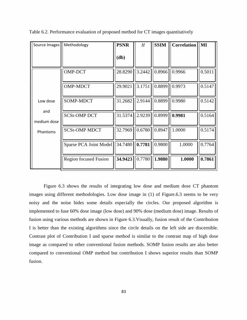
83


Source Images Methodology PSNR

(db)

SSIM Correlation MI

Low dose

and

medium dose

Phantoms

OMP-DCT 28.8290 3.2442 0.8966 0.9966 0.5011

OMP-MDCT 29.9021 3.1751 0.8899 0.9973 0.5147

SOMP-MDCT 31.2682 2.9144 0.8899 0.9980 0.5142

SCSt-OMP DCT 31.5374 2.9239 0.8999 0.9981 0.5164

SCSt-OMP MDCT 32.7969 0.6780 0.8947 1.0000 0.5174

Sparse PCA Joint Model 34.7480 0.7781 0.9800 1.0000 0.7764

Region focused Fusion 34.9423 0.7780 1.9880 1.0000 0.7861

Figure 6.3 shows the results of integrating low dose and medium dose CT phantom

images using different methodologies. Low dose image in (1) of Figure.6.3 seems to be very

noisy and the noise hides some details especially the circles. Our proposed algorithm is

implemented to fuse 60% dose image (low dose) and 90% dose (medium dose) image. Results of

fusion using various methods are shown in Figure 6.3.Visually, fusion result of the Contribution

I is better than the existing algorithms since the circle details on the left side are discernible.

Contrast plot of Contribution I and sparse method is similar to the contrast map of high dose

image as compared to other conventional fusion methods. SOMP fusion results are also better

compared to conventional OMP method but contribution I shows superior results than SOMP

fusion.

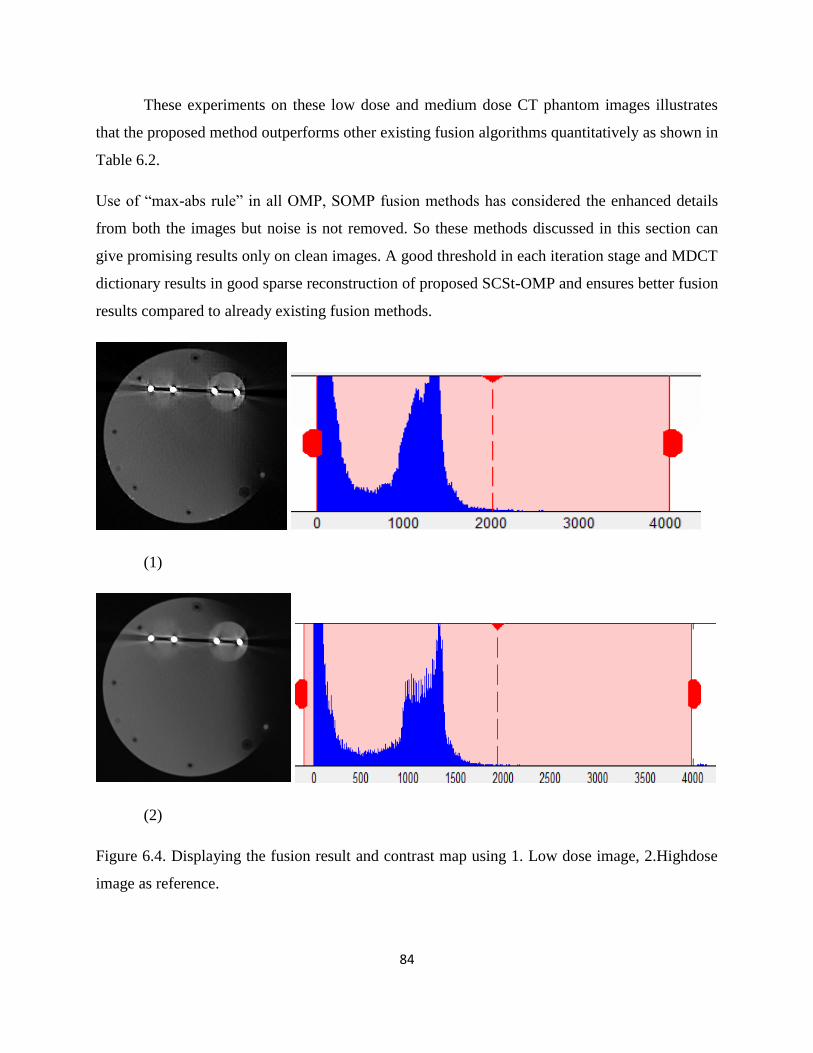
84

These experiments on these low dose and medium dose CT phantom images illustrates

that the proposed method outperforms other existing fusion algorithms quantitatively as shown in

Table 6.2.

Use of “max-abs rule” in all OMP, SOMP fusion methods has considered the enhanced details

from both the images but noise is not removed. So these methods discussed in this section can

give promising results only on clean images. A good threshold in each iteration stage and MDCT

dictionary results in good sparse reconstruction of proposed SCSt-OMP and ensures better fusion

results compared to already existing fusion methods.

(1)

(2)


image as reference.

85

(3)

(4)

(5)

Figure 6.4. Displaying the fusion result and contrast map using 3.OMP-MDCT, 4. SCSt-OMP

utilizing Overcomplete DCT and 5. SCSt-OMP utilizing MDCT.

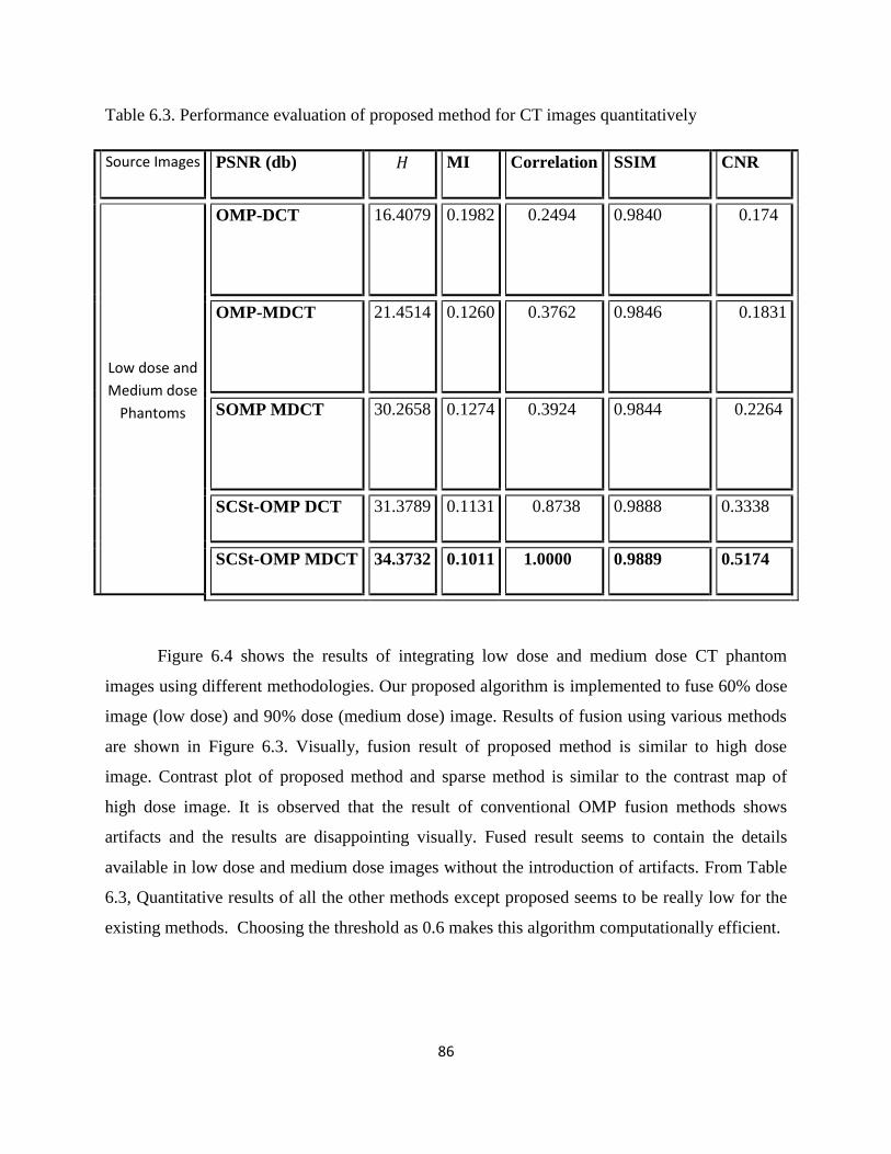
86


Source Images PSNR (db) MI Correlation SSIM CNR

Low dose and

Medium dose

Phantoms

OMP-DCT 16.4079 0.1982

0.2494

0.9840

0.174

OMP-MDCT 21.4514 0.1260

0.3762

0.9846 0.1831

SOMP MDCT 30.2658

0.1274

0.3924

0.9844 0.2264

SCSt-OMP DCT 31.3789 0.1131 0.8738 0.9888 0.3338

SCSt-OMP MDCT 34.3732 0.1011 1.0000 0.9889 0.5174

Figure 6.4 shows the results of integrating low dose and medium dose CT phantom

images using different methodologies. Our proposed algorithm is implemented to fuse 60% dose

image (low dose) and 90% dose (medium dose) image. Results of fusion using various methods

are shown in Figure 6.3. Visually, fusion result of proposed method is similar to high dose

image. Contrast plot of proposed method and sparse method is similar to the contrast map of

high dose image. It is observed that the result of conventional OMP fusion methods shows

artifacts and the results are disappointing visually. Fused result seems to contain the details

available in low dose and medium dose images without the introduction of artifacts. From Table

6.3, Quantitative results of all the other methods except proposed seems to be really low for the

existing methods. Choosing the threshold as 0.6 makes this algorithm computationally efficient.

87

6.3. Experimental setup and Results of Contribution II and Contribution III

Under this section, the experiments are performed on low dose and medium dose CT

images using proposed Joint Sparse PCA and fusion using focused vector. As similar to previous

section, the same five evaluation criteria are used to assess the quality of the fused image.

Learning-based dictionaries are used for efficient sparse representation than fixed dictionaries.

We use a patch size of and the dictionary learned from high dose images has the size

. For the noise intensity of , we set the stopping error criterion as .

(1)

Figure 6.5. Displaying the fusion result and contrast map using 1. Low dose image (source image)

88

(2)

(3)

Figure 6.5. Displaying the fusion result and contrast map using 1. Low dose image (source image),

2.Medium dose image (source image), 3. High dose image (reference image).

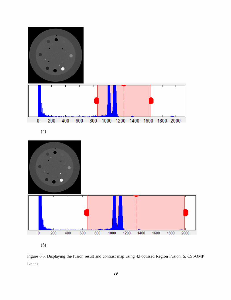
89

(4)

(5)

Figure 6.5. Displaying the fusion result and contrast map using 4.Focussed Region Fusion, 5. CSt-OMP

fusion

90

(6)

Figure 6.5. Displaying the fusion result and contrast map using 6. Joint Sparse PCA fusion


Source Images PSNR (db) MI Correlation SSIM CNR

Low dose and

Medium dose

Phantoms

CSt-OMP fusion 27.7356 0.0357 0.999

0.9609

23.4655

Joint Sparse PCA

fusion

27.7925 0.0418

0.999

0.9644 22.5055

Focused Region

fusion

29.5398 0.035 1.0000 0.9777

20.5025

Figure 6.3 (6) and (7) are the fused images of Joint Sparse PCA fusion and Region

focused image fusion methods. All the details are clearly discernible. Especially the circular

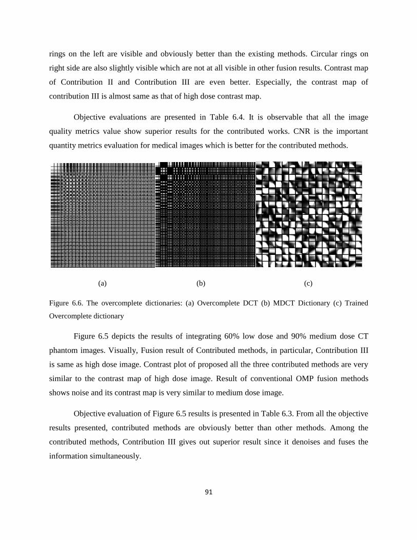
91

rings on the left are visible and obviously better than the existing methods. Circular rings on

right side are also slightly visible which are not at all visible in other fusion results. Contrast map

of Contribution II and Contribution III are even better. Especially, the contrast map of

contribution III is almost same as that of high dose contrast map.

Objective evaluations are presented in Table 6.4. It is observable that all the image

quality metrics value show superior results for the contributed works. CNR is the important

quantity metrics evaluation for medical images which is better for the contributed methods.

(a) (b) (c)

Figure 6.6. The overcomplete dictionaries: (a) Overcomplete DCT (b) MDCT Dictionary (c) Trained

Overcomplete dictionary

Figure 6.5 depicts the results of integrating 60% low dose and 90% medium dose CT

phantom images. Visually, Fusion result of Contributed methods, in particular, Contribution III

is same as high dose image. Contrast plot of proposed all the three contributed methods are very

similar to the contrast map of high dose image. Result of conventional OMP fusion methods

shows noise and its contrast map is very similar to medium dose image.

Objective evaluation of Figure 6.5 results is presented in Table 6.3. From all the objective

results presented, contributed methods are obviously better than other methods. Among the

contributed methods, Contribution III gives out superior result since it denoises and fuses the

information simultaneously.

92

6.4. Integration of unregistered images using Focused Region fusion

To confirm the effective performance of the focused region based sparse fusion, further,

unregistered low dose images of the same region of interest is fused. The fused result is

evaluated using Contrast Noise Ratio (CNR) and contrast map. Maximum iteration of K-SVD is

set to 40. High dose resolution CT set is incorporated during the training process for enhancing

the details and the trained dictionary is shown in Figure 6.6.(c). Source images are two Cone

Beam CTs (CBCT) of the same patient at two different times. The goal is to denoise the CBCTs

using the high resolution CT as learning set.

(1)

Figure 6.7. Displaying the fusion result and Contrast map of fusing two Cone Beam CTs (CBCT) 1. Low

dose image with CNR 22.8330

93

(2)

(3)

Figure 6.7. Displaying the fusion result and Contrast map of fusing two Cone Beam CTs (CBCT) 2.

Another low dose image with CNR of 22.1172, 3.Fusion result of proposed method with CNR of 21.4806

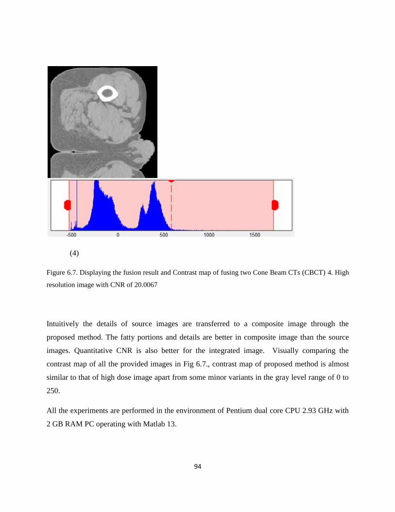
94

(4)

Figure 6.7. Displaying the fusion result and Contrast map of fusing two Cone Beam CTs (CBCT) 4. High

resolution image with CNR of 20.0067

Intuitively the details of source images are transferred to a composite image through the

proposed method. The fatty portions and details are better in composite image than the source

images. Quantitative CNR is also better for the integrated image. Visually comparing the

contrast map of all the provided images in Fig 6.7., contrast map of proposed method is almost

similar to that of high dose image apart from some minor variants in the gray level range of 0 to

250.

All the experiments are performed in the environment of Pentium dual core CPU 2.93 GHz with

2 GB RAM PC operating with Matlab 13.

95

Chapter 7. Conclusion and Future

Works

7.1. Image fusion with simultaneous controlled orthogonal matching pursuit

Medical Image fusion plays a vital role in clinical diagnosis. We proposed a simultaneous

sparse fusion method where the images are integrated in sparse domain. Sparse coding and

fusion process is done parallelly by simultaneous controlled orthogonal matching pursuit (SCSt-

OMP) utilizing MDCT dictionary. Experiments are done in low dose and medium dose images

to check the performance of the proposed method and results are compared with the conventional

sparse fusion methods and SOMP fusion method. Based on the qualitative and quantitative

analysis, the proposed method produces superior results than SOMP fusion method and OMP

fusion method. Use of SCSt-OMP methods increases the computational efficiency since each

stage allows multiple atoms but sliding window technique makes the process slightly time

consuming. Even though the fusion results are superior, this fusion assumes the source images to

be noiseless. But source images are prone to noise and for noisy images, the fused result will

have reduced PSNR. Tuning the error stopping criterion with respect to the noise intensity would

be the ideal idea for further improvement.

96

7.2. Image fusion with Joint Sparse Fusion

Another method based on Joint Sparse Representation (JSR) is aimed to effectively integrate

multi-dosage images to enhance the details necessary for diagnosis. This framework makes use

of the proposed SCSt-OMP method for simultaneous sparse coding in JSR. And PCA fusion is

used to integrate the innovative component sparse vector. It’s necessary to note that many fusion

algorithms are developed with the assumption that the source images are noise free. Since our

algorithm is experimented on multi-dosage images, low dose CT images are prone to noise.

Unlike traditional fusion methods, the proposed Joint Sparse fusion method simultaneously fuses

and denoises the image by tuning the error threshold with respect to the noise intensity. Visually

and quantitatively, the experimental results show that the proposed method has effectively

expressed the geometric structures and edges and has proved to outperform some of the state-of-

the-art fusion algorithms. Objective results and contrast map shows that combination of PCA

fusion and weighted average fusion works great for fusing multi-dosage images than the other

combinations.

7.3. Fusion based on Focused Vector

In this paper a novel sparse image fusion method is proposed for fusing low dose CT images

based on focused vector. This method is the extension of the proposed Joint Sparse PCA fusion

method where fusion result is constructed from initial fused image and focused vector. In this

method, sparse coding stage utilizes a dictionary trained from high resolution CT images and

denoises the low dose image by fusing low dose and medium dose CT images in sparse domain.

The results of the proposed method outperform all the other existing fusion methods presented

here in terms of qualitative and quantitative measurements when tested on both noisy and

noiseless images. Contrast map the fusion result of this proposed method is almost same as high

dose image. This framework effectively fuses the information without the introduction of

artifacts, transfers the details from source images to composite image, suppresses noise without

losing any detail. The dictionary used here is trained off-line. This work can be further refined

exploiting dictionaries that are trained so that they will be suitable for different source images.

97

References

[1] S.Mallat, “A wavelet tour of signal processing”, Academic Press, 1999.

[2] EricWeisstein.MathWorld[Online]: http://mathworld.wolfram.com/MoorePenroseMatrixInverse.html

[3] T. Strohmer, and R. Heath Jr, “ Grassmannian frames with applications to coding and

communications”, Appl. Comp. Harm. Anal., vol.14(3): 257--275, 2003.

[4] David L. Donoho, Michael Elad ,“Optimally sparse representation in general (nonorthogonal)

dictionaries via minimization”, Proceedings of the National Academy of Sciences, Vol. 100, No. 5. (04

March 2003), pp. 2197-2202.

[5] Tibshirani. R, “Regression shrinkage and selection via the lasso.”, Vol. 58, No. 1, pp. 267-288., 1996

[6] Simon Perkins , James Theiler, “Online Feature Selection Using Grafting “, International Conference

on Machine Learning 2013.

[7] Jinseog Kim, Yuwon Kim and Yongdai Kim,” A gradient-based optimization algorithm for

lasso”, Journal of Computational and Graphical Statistics Volume 17, Issue 4, 2008.

[8] Tropp, J.A.,“Greed is good: algorithmic results for sparse approximation”, Information Theory, IEEE

Transactions on (Volume:50 , Issue: 10 , Page: 2231 - 2242), Oct. 2004.

[9] Mallat, S.G. ,“Matching pursuits with time-frequency dictionaries”, Signal Processing, IEEE

Transactions on (Volume:41 , Issue:12, Page: 3397 - 3415 ), Dec. 1993.

[10] S. Chen, S.A. Billings and W. Luo, "Orthogonal least squares methods and their application to non-

linear system identification," International Journal of Control, vol. 50, no. 5, pp. 1873-1896, 1989.

[11] Y.C. Pati, R. Rezaiifar and P.S. Krishnaprasad, "Orthogonal matching pursuit: recursive function

approximation with applications to wavelet decomposition," Conference Record of The Twenty

Seventh Asilomar Conference on Signals, Systems and Computers, 1993.

[12] David L. Donoho , Yaakov Tsaig , Iddo Drori , Jean-luc Starck,“Stage wise Orthogonal Matching

Pursuit”, IEEE Transactions on Information Theory, January 2012; 58:1094-1121

[13] Ahmed, N, Natarajan, T, Rao K. R, "Discrete Cosine Transform", IEEE Transactions on Computers

C–23 (1), pp. 90–93, January 1974.

[14] M. N. Do and M. Vetterli, “The contourlet transform: an efficient directional multiresolution image

representation”, IEEE Transactions on Image Processing, vol. 14, no. 12, pp. 2091–2106, Dec. 2005.

[15] Rubinstein, R., “Dictionaries for Sparse Representation Modeling”, Proceedings of the

IEEE (Volume:98 , Issue: 6 ,pp. 1045 - 1057), June 2010.

[16] Michal Aharon, Michael Elad, and Alfred Bruckstein (2006), "K-SVD: An Algorithm for Designing

Overcomplete Dictionaries for Sparse Representation", pp. 4311 - 4322.

http://www-stat.stanford.edu/~tibs/lasso/lasso.pdf

http://ieeexplore.ieee.org/search/searchresult.jsp?searchWithin=p_Authors:.QT.Tropp,%20J.A..QT.&searchWithin=p_Author_Ids:37273007000&newsearch=true

http://ieeexplore.ieee.org/xpl/RecentIssue.jsp?punumber=18


http://ieeexplore.ieee.org/xpl/tocresult.jsp?isnumber=29493

http://ieeexplore.ieee.org/search/searchresult.jsp?searchWithin=p_Authors:.QT.Mallat,%20S.G..QT.&newsearch=true




http://www.researchgate.net/journal/0018-9448_IEEE_Transactions_on_Information_Theory

http://ieeexplore.ieee.org/search/searchresult.jsp?searchWithin=p_Authors:.QT.Rubinstein,%20R..QT.&searchWithin=p_Author_Ids:37391099500&newsearch=true




http://intranet.daiict.ac.in/~ajit_r/IT530/KSVD_IEEETSP.pdf

http://intranet.daiict.ac.in/~ajit_r/IT530/KSVD_IEEETSP.pdf

98

[17] S. Mallat, “A Wavelet Tour of Signal Processing”, 2nd ed. San Diego, CA: Academic, 1999.

[18] N. G. Kingsbury, "Complex wavelets for shift invariant analysis and filtering of signals," Applied

and Computational Harmonic Analysis, no. 10, pp. 234-252, 2001.

[19] Olshausen BA, and Field DJ. (1996). "Emergence of Simple-Cell Receptive Field Properties by

Learning a Sparse Code for Natural Images." Nature, 381: 607-609.

[20] K. Engan, S. O. Aase, J. H. Husoy, “Method of Optimal Directions for Frame Design,” in Proc.

ICASSP’99, Phoenix, USA, pp. 2443--2446, March, 1999.

[21] K. Engan, B. Rao, and K. Kreutz-Delgado, “Frame design using FOCUSS with method of optimized

directions (MOD)”, in Proc. NORSIG ‘99, Oslo, Norway, Sept. 1999, pp. 65--69.

[22] Ren Ng, Ravi Ramamoorthi, Pat Hanrahan,“Triple product wavelet integrals for all-frequency

relighting”, ACM Transactions on Graphics (TOG) - Proceedings of ACM SIGGRAPH 2004, Volume 23

Issue 3, August 2004 Pages 477-487.

[23] Chui, Charles K. (1992). “An Introduction to Wavelets.” San Diego: Academic Press.

[24] Michael Elad, “Sparse and Redundant Representations: From Theory to Applications in Signal and

Image Processing”, Springer, August 2010.

[25] Ishita Dea, Bhabatosh Chandab, "A simple and efficient algorithm for multifocus image fusion using

morphological wavelets", Journal Signal Processing archive Volume 86 Issue 5,Pages 924-936, May

2006.

[26] A. Goshtasby and C. Page, "A Multiple Image Segmentation Technique with Subpixel Accuracy,"

Proc. Computer Vision and Pattern Recognition, 1983, pp. 157-158.

[27] A. Goshtasby, "Registration of Images with Geometric Distortions," IEEE Trans. Geoscience and

Remote Sensing, vol. 26, no. 1, 1988, pp. 60-64.

[28] L. Kitchen, A. Rosenfeld, "Gray-level corner detection" Pattern Recognition Lett. , 1 : 2 (1982) pp.

95–102.

[29] L. Zagorchev and A. Goshtasby, "A comparative study of transformation functions for nonrigid

image registration," IEEE Trans. Image Processing, vol. 15, no. 3, 2006, 529-538.

[30] Deubel, H. and Schneider, W.X.(1996),”Saccade target selection and object recognition: evidence for

a common attentional mechanism.”, Vision Res., 36: 1827–1837.

[31] Ardeshir Goshtasby, A; Nikolov, SG,”Image fusion: Advances in the state of the art.”, Information

Fusion: Special Issue on Image Fusion: Advances in the State of the Art, Vol. 8 (2), 04.2007, pp. 114 -

118.

[32] Gemma Piella, “A general framework for multiresolution image fusion: from pixels to regions.”,

Information Fusion 4 (4), pp. 259-280, 586, 2003.

[33] R. A. Brooks and G. DiChiro, “Principles of computer assisted tomography (CAT) in radiographic

and radioisotopic imaging,” Phys. Med. Biol., vol. 21, pp. 689- 732, 1976.

http://www.google.de/search?hl=de&tbo=p&tbm=bks&q=inauthor:%22Michael+Elad%22

99

[34] Tinsu Pan, “Computed Tomography: from Photon Statistics to Modern Cone-Beam CT”, The

Journal of Nuclear Medicine, 2009;50:1194.

[35] Cormack AM,” Early two-dimensional reconstruction and recent topics stemming from it.”, Med

Phys 7(4):277. Nobel Lecture, 8 December, 1979.

[36] Hounsfield, GN. 1973. “Computerized transverse axial scanning (tomography): Part I”, Brit J Radiol

46:1016–1022.

[37] Kak A. and Slaney Malcolm,”Principles of Computed Tomography Imaging”, 1988.

[38] Mikael Sandborg ,“Computed Tomography: Physical principles and biohazards ”, Report /

Department of Radiology, Linköping University, 1990-1997, ISSN 1102-1799; 81.

[39] Jones DG, Shrimpton P C,” Survey of CT practice in the UK Part 3: Normalised organ doses

calculated using Monte Carlo techniques”, National Radio logical Protection Board, Chilton, United

Kingdom 1991; NRPB-R250.

[40] ICRP, International Commission on Radiological Protection. 1990 Recommendations of the

International Commission on Radiological Protection. 1991; Annals of the ICRP, Publication 60, Oxford:

Pergamon.

[41] National Council on Radiation Protection & Measurements, “Report No. 160 - Ionizing Radiation

Exposure of the Population of the United States (2009)”.

[42] Borsdorf, A., FriedrichAlexander, Raupach, R. , Hornegger, J. ,“Separate CT-reconstruction for 3D

wavelet based noise reduction using correlation analysis”, Nuclear Science Symposium Conference

Record, 2007. NSS '07. IEEE,P: 2633 – 2638.

[43] Hu H, He HD, Foley WD, Fox SH,”Four multidetector-row helical CT: image qualityand volume

coverage speed”, Radiology 2000; pp.55-62.

[44] http://www.iambiomed.com/equipments/ct.php

[45] A. Saleem, A. Beghdadi and B. Boashash,” Image fusion-based contrast enhancement”, Journal on

Image and Video Processing, 2012, pp.1-17.

[46] Y. Zhou, “Principle Component Analysis Based image Fusion Routine with Application to Stamping

Split Detection”, Ph.D. dissertation, Dept. of Automotive Engineering , University of Clemson, August

2010, pp. 76-91.

[47] M. R.Metwalli, A.H. Nasr, O. S. Farag Allah, and S. El-Rabaie, ”Image fusion based on Principal

Component Analysis and High-pass Filter”, Presented at IEEE/ ICCES 2009 international Conference,

Dec. 14-16,2009, pp. 63 - 70.

[48] H. Yin, S. Li,” Multimodal image fusion with joint sparsity model”, Opt Eng, 2011.

[49]B. Yang and S. Li,Multifocus Image Fusion and Restoration With Sparse Representation, IEEE

transactions on Instrumentation and Measurement, Vol. 59, No. 4, April 2010, pp. 884–892.

[50] http://bigwww.epfl.ch/sage/soft/snr/.

http://www.iambiomed.com/equipments/ct.php

100

[51] Junli Tao, Shutao Li, Bin Yang, “Multimodal Image Fusion Algorithm Using Dual-Tree Complex

Wavelet Transform and Particle Swarm Optimization”, 6th International Conference on Intelligent

Computing, ICIC 2010, Changsha, China, August 18-21, 2010.

[52] Bin Yang, Shutao Li ,“Pixel-level image fusion with simultaneous orthogonal matching pursuit”,

Information FusionVolume 13, Issue 1, January 2012, pp.10–19.

[53] Hui Li, Manjunath, Mitra.S.K,”Multi-sensor image fusion using the wavelet transform”, Image

Processing, 1994. Proceedings. ICIP-94., IEEE International Conference Volume:1, pp: 51 – 55.

[54] Xydeas, C.S., Petrovic. V.,“ Objective image fusion performance measure”, Electronics Letters

(Volume:36 , Issue: 4 ),pp:308-309.

[55] Zhou Wang, Bovik, A.C., Sheikh, H.R., Simoncelli.E.P.,”Image Quality Assessment: From Error

Visibility to Structural Similarity”, Image Processing, IEEE Transactions on Volume:13, Issue:4 ,

pp:600-612.

[56] CJ Martin, “The importance of radiation quality for optimisation in radiology”, Biomedical Imaging

and Intervention Journal, 2007, pp. e38.

[57] S.G. Nikolov., P.R. Hill., D.R. Bull., C.N. Canagarajah., "Wavelets for image fusion", A. Petrosian,

F. Meyer (Eds.), Wavelets in Signal and Image Analysis, Computational Imaging and Vision Series,

Kluwer Academic Publishers, Dordrecht, The Netherlands (2001). pp. 213–244.

[58] P. Burt, R. Kolczynski,"Enhanced image capture through fusion", Proceedings of the 4th

International Conference on Computer Vision, 1993, pp. 173-182.

[59] L. Rebollo‐Neira and D. Lowe, "Optimized orthogonal matching pursuit approach,"IEEE Signal

Processing Letters, pp.137–140, 2002.

[60] Qiheng Zhang ; Yuli Fu ; Haifeng Li ; Jian Zou ,“Dictionary learning method for joint sparse

representation-based image fusion”, Opt. Eng. 52(5), 057006 (May 22, 2013), pp. 1-11.

[61] Aline Bonami,Bruno Demange, and Philippe Jaming, “Hermite functions and uncertainty principles

for the Fourier and the windowed Fourier transforms”,Volume 19,2003, pp. 23-55.

[62] M. F. Duarte, S. Sarvotham, D. Baron, M. B. Wakin, and R. G. Baraniuk, “Distributed Compressed

Sensing of Jointly Sparse Signals”, Proceedings of the 39th Asilomar Conference on Signals, Systems

and Computation, 2005, pp.1537-1541.

101

List of Publications

1. Anuyogam Venkataraman, Javad Alirezaie, Paul Babyn and Alireza Ahmadian, “Medical Image

Fusion Based on Joint Sparse Method”, 2nd Middle East Conference on Biomedical Engineering,

February 2014, pp. 103-106.

2. Anuyogam Venkataraman, Javad Alirezaie, Paul Babyn and Alireza Ahmadian, “Multi dose

Computed Tomography Image Fusion Based on Hybrid Sparse Methodology”, accepted in 36th

Annual International IEEE EMBS Conference 2014 to, Chicago, Illinois, USA.

computed tomography image denoising...

Documents