comparison between heidler function and the pulse...
TRANSCRIPT

Ryerson UniversityDigital Commons @ Ryerson
Theses and dissertations
1-1-2010
Comparison Between Heidler Function And ThePulse Function For Modeling The LightningReturn-Stroke CurrentKhaled ElrodeslyRyerson University
Follow this and additional works at: http://digitalcommons.ryerson.ca/dissertationsPart of the Electrical and Computer Engineering Commons
This Thesis is brought to you for free and open access by Digital Commons @ Ryerson. It has been accepted for inclusion in Theses and dissertations byan authorized administrator of Digital Commons @ Ryerson. For more information, please contact [email protected].
Recommended CitationElrodesly, Khaled, "Comparison Between Heidler Function And The Pulse Function For Modeling The Lightning Return-StrokeCurrent" (2010). Theses and dissertations. Paper 1323.
Comparison between Heidler Function and
the Pulse Function for Modeling the
Lightning Return-Stroke Current
By
Khaled Elrodesly
Bachelor of Science
Electronics and Electrical Communications Engineering
Ain Shams University, Cairo, Egypt, 2008
A thesis
presented to Ryerson University
in partial fulfillment of the
requirements for the degree of
Master of Applied Science
in the Program of
Electrical and Computer Engineering
Toronto, Ontario, Canada, 2010
©Khaled Elrodesly, 2010

ii
AUTHOR DECLARATION
I hereby declare that I am the sole author of this thesis or dissertation.
I authorize Ryerson University to lend this thesis or dissertation to other institutions or
individuals for the purpose of scholarly research.
Khaled Elrodesly
---------------------
I further authorize Ryerson University to reproduce this thesis or dissertation by
photocopying or by other means, in total or in part, at the request of other institutions or
individuals for the purpose of scholarly research.
Khaled Elrodesly
---------------------

iii
ABSTRACT
Comparison between Heidler Function and the Pulse Function for Modeling Lightning
Return-Stroke Current
Master of Applied Science, 2010
Khaled Elrodesly
Electrical and Computer Engineering
Ryerson University
In the past, many functions were considered for simulating the lightning return-
stroke current. Some of these functions were found to have problems related to their
discontinuities or the discontinuities of their derivatives at onset time. Such problems
appear in the double exponential function and its modifications. However, other functions
like the Pulse function and Heidler function do not suffer from such problems.
One of the main objectives of this work is to simulate the lightning return-stroke
current full wave, including the decay part, using either Heidler function or the Pulse
function. This work is not only necessary for the evaluation and development of lightning
return-stroke modeling, but also for the calculation of the lightning current waveform
parameters.
Although the lightning return-stroke current, measured at the CN Tower, is
simulated using the Pulse function and Heidler function, the simulation of the CN Tower
lightning current derivative signal is considered using the derivative of the Pulse and
Heidler functions.

iv
First, we build a modeling environment for each function, which can be described
as parameter estimation system. This system, which represents an automated approach
for estimating the analytical parameters of a given function, is capable to best fit the
function with the measured data. Using these analytical parameters transforms the
discrete data into a continuous signal, from which the current waveform parameters can
be estimated.
This analytical parameters estimation system is recognized as a curve fitting
system. For curve fitting technique, the initial value of each analytical parameter and its
feasible region, where the optimal value of this analytical parameter is located, must be
specified. The more accurate the initial point is the easier and faster the optimal value can
be estimated. On choosing the best approach of the initial condition, which gives the
nearest location to the optimal point, applying the estimation system and achieving the
analytical model that fits the CN Tower measured current derivative, the current
waveform parameters can be easily studied.
In order to be sure that the analytical parameter extraction system gives the best
fit of a function, it needs to be evaluated. Instead of going through the measured data, we
first use artificial digital data as a productive way to evaluate the system. Also, a
comparison between both the Pulse and Heidler functions is performed.
The described fitting process is applied on 15 flashes, containing 31 return
strokes. The calculated current waveform parameters were used to form statistics to
determine the probability distribution of the value of each parameter, including the range
and the 50% probability level, which is fundamental in building lightning protection
systems.

v
ACKNOWLEDGEMENTS
I feel deeply indebted to my supervisor, Professor Dr. Ali Hussein, for his
patience, guidance, constant supervision, creative advising and personal involvement
throughout the progression of this work. He has been, for me, not only a source of
inspiration and encouragement but also a model of ideal academic relations. Much of
what I have learned during the progress of this thesis I owe, in fact, to Professor Hussein.
Working under the supervision of a very great investigator of the highest academic and
human caliber like Professor Hussein has formed me and will continue to be an
unforgettable and a unique experience of my life.
I would like to express my great appreciation and gratitude to Dr. Kaamran
Raahemifar for his guidance, advice and moral support. My thanks go to all my
Professors at Ryerson University who taught me during my graduate study at the
University.
I am thankful to the Department of Electrical and Computer Engineering, Ryerson
University for offering all facilities, financial resources and the academic environments
that made this work possible
I would like to express my deepest appreciation to my parents and brother for
their moral support, patience and unconditional love.

vi
TABLE OF CONTENTS
1. CHAPTER 1: INTRODUCTION ...................................................................... 1
2. CHAPTER 2: LIGHTNING PHYSICS ........................................................... 5
2.1 ELECTRIFICATION OF THUNDERSTORMS ...................................................7
2.1.1 Precipitation Thesis ................................................................................................. 8
2.1.2 Convection Thesis .................................................................................................. 9
2.1.3 Tri-pole Modification ............................................................................................. 9
2.2 LIGHTNING CATEGORIES ...............................................................................11
2.2.1 Cloud-to-cloud ..................................................................................................... 11
2.2.2 Cloud to earth ....................................................................................................... 11
2.3 LIGHTNING FORMATION ................................................................................13
2.4 LIGHTNING TO TALL STRUCTURES ............................................................14
2.5 CN TOWER AND ITS MEASUREMENT SYSTEM .........................................16
2.6 CURRENT WAVEFORM PARAMETERS .........................................................21
3. CHAPTER 3: SIMULATING FUNCTIONS .............................................. 23
3.1 DOUBLE EXPONENTIAL FUNCTION .............................................................24
3.2 JONES MODIFICATION .....................................................................................27
3.3 HEIDLER FUNCTION .........................................................................................32
3.4 PULSE FUNCTION ..............................................................................................44
4. CHAPTER 4: CURRENT FITTING TECHNIQUE ................................ 51
4.1 CURVE FITTING ................................................................................................51
4.1.1 Least Square Regression ....................................................................................... 52

vii
4.1.2 Non Linear Regression ......................................................................................... 54
4.1.3 Goodness of the Fit ............................................................................................... 57
4.2 MODELING ENVIRONMENT ...........................................................................58
4.2.1 Artificial Signal Concept ...................................................................................... 58
4.2.2 Modeling Using Artificial Signal ......................................................................... 60
4.3 INITIAL CONDITION .........................................................................................68
4.3.1 Initial Condition for the Pulse Function ............................................................... 68
4.3.2 Initial Condition for Heidler Function .................................................................. 75
5. CHAPTER 5:RESULTS AMD DISCUSSIONS ......................................... 82
5.1 ESTIMATING τ2 ..................................................................................................86
5.2 ESTIMATING IMAX ...............................................................................................91
5.3 APPLYING CONSTRAINTS ..............................................................................92
5.3.1 Condition of Current Derivative Zero Crossing .................................................. 93
5.3.2 Time of Maximum Steepness Condition ............................................................. 96
5.4 CURRENT WAVEFORM PARAMETERS ........................................................99
5.5 Cumulative Distripution ......................................................................................100
5.5.1 Current Peak ....................................................................................................... 100
5.5.2 Maximum Steepness .......................................................................................... 101
5.5.3 Risetime to the Current Peak .............................................................................. 102
5.5.4 Decay time from the Current Peak .................................................................... 103
5.5.5 Current Pulse Width .......................................................................................... 104
5.5.6 Charge ................................................................................................................ 105
6. CHAPTER 6: CONCLUSIONS AND RECOMMENDATIONS ....... 107
REFERENCES ......................................................................................................... 109

viii
List of Figures
Figure 2.1: Earth-Atmosphere charge .................................................................................6
Figure 2.2: World map showing frequency of Lightning ...................................................7
Figure 2.3: Dipole Models ..................................................................................................8
Figure 2.4: Precipitation Thesis ..........................................................................................8
Figure 2.5: Convection Thesis ............................................................................................9
Figure 2.6: Charge Reversal Temperature ........................................................................10
Figure 2.7: Different types of lightning ............................................................................11
Figure 2.8: Lighting Formation Process ...........................................................................14
Figure 2.9: Branching of upward-initiated lightning ........................................................15
Figure 2.10: CN Tower and its surrounding .....................................................................17
Figure 2.11: CN Tower and the lightning measurement location .....................................18
Figure 2.12: Schematic of old Rogowski coil connection ................................................19
Figure 2.13: Schematic of new Rogowski coil connection ...............................................20
Figure 2.14: Demonstration of current maximum steepness ............................................22
Figure 2.15 Demonstration of current peak and risetime of current .................................22
Figure 3.1: Current simulation using double exponential function with I = 10 kA, τ1 = 5
µs and τ2 = 0.5 µs ..............................................................................................................24
Figure 3.2: Current Derivative simulation using double exponential derivative function
with I = 10 kA, τ1 = 5 µs and τ2 = 0.5 µs ..........................................................................26
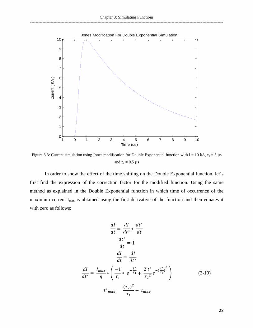
Figure 3.3: Current simulation using Jones modification for double exponential function
with I = 10 kA, τ1 = 5 µs and τ2 = 0.5 µs ..........................................................................28
Figure 3.4: Current Derivative simulation using double exponential derivative function
with I = 10 kA, τ1 = 5 µs and τ2 = 0.5 µs ..........................................................................30

ix
Figure 3.5: Current simulation using double exponential and Jone modification for double
exponential derivative function with I = 10 kA, τ1 = 5 µs and τ2 = 0.5 µs .......................31
Figure 3.6: Current Derivative simulation using double exponential and Jone
modification for double exponential derivative function with I = 10 kA, τ1 = 5 µs and τ2 =
0.5 µs .................................................................................................................................31
Figure 3.7: Current simulation using Heidler function with I = 10 kA, τ1 = 0.3 µs, τ2 = 3
us and n = 7 .......................................................................................................................37
Figure 3.8: Current derivative simulation using Heidler derivative function with I = 10
kA, τ1 = 0.3 µs, τ2 = 3 µs and n = 7 ..................................................................................38
Figure 3.9: Current simulation using Pulse function with I = 10 kA, τ1 = 0.5 µs, τ2 = 10
µs and n = 5 ........................................................................................................................45
Figure 3.10: Current derivative simulation using Pulse function derivative with I = 10 kA,
τ1 = 0.5 µs, τ2 = 10 µs and n = 5 ........................................................................................47
Figure 4.1: Example of the criteria for “best fit” based on minimizing the sum of the
residual ..............................................................................................................................52
Figure 4.2: Example of the criteria for “best fit” based on minimizing the sum of the
absolute value of the residual ............................................................................................53
Figure 4.3: Example of the criteria for “best fit” based on minimizing the maximum error
of any individual point ......................................................................................................54
Figure 4.4: Artificial signal production simulation for current and current derivative with
rate 10 ns ...........................................................................................................................60
Figure 4.5: Curve fitting results using Pulse function artificial signal with I = 10 kA, τ1 =
0.07 µs, τ2 = 1 µs and n =6 .................................................................................................61
Figure 4.6: Curve fitting results using Heidler function artificial signal with I = 10 kA, τ1
= 0.1 µs, τ2 =2 µs and n =5 ...............................................................................................62
Figure 4.7: Current fitting results using Pulse current function and the corresponding
current derivative simulation with Heidler artificial signal of parameters I = 10 kA, τ1 =
0.1 µs, τ2 = 2 µs and n = 5 .................................................................................................63

x
Figure 4.8: Current derivative fitting results using Pulse current derivative function and
the corresponding current simulation with Heidler artificial signal of parameters I = 10
kA, τ1 = 0.1 µs, τ2 = 2 µs and n = 5 ..................................................................................64
Figure 4.9: Current derivative fitting results using Pulse current derivative function and
the corresponding current simulation with Heidler artificial signal of parameters I = 10
kA, τ1 = 0.1 µs, τ2 = 2 µs and n = 5 ...................................................................................65
Figure 4.10: Current derivative fitting results using Heidler current derivative function
and the corresponding current simulation with Pulse artificial signal of parameters I = 10
kA, τ1 = 0.07 µs, τ2 = 1 µs and n = 6 .................................................................................66
Figure 4.11: Current fitting results using Heidler current function and the corresponding
current simulation with Pulse artificial signal of parameters I = 10 kA, τ1 = 0.07 µs, τ2 = 1
µs and n = 6 ........................................................................................................................67
Figure 4.12: Relative error value for the estimated values of τ1, τ2 and n with the change
of its value individually using the Pulse function initial condition estimation .................72
Figure 4.13: Relative error value for the estimated values of n with the change of τ1 and
τ2 using the Pulse function initial condition estimation ....................................................73
Figure 4.14: Relative error value for the estimated values of τ2 with the change of τ1 and
n using the Pulse function initial condition estimation .....................................................73
Figure 4.15: Relative error value for the estimated values of τ1 with the change of τ2 and
n using the Pulse function initial condition estimation .....................................................74
Figure 4.16: Relative error value for the estimated values of τ1, τ2 and n with the change
of its value individually using Heidler function initial condition estimation ...................79
Figure 4.17: Relative error value for the estimated values of n with the change of τ1 and
τ2 using Heidler function initial condition estimation ......................................................80
Figure 4.18: Relative error value for the estimated values of τ2 with the change of τ1 and
n using Heidler function initial condition estimation .......................................................80
Figure 4.19: Relative error value for the estimated values of τ1 with the change of τ2 and
n using Heidler function initial condition estimation .......................................................80

xi
Figure 5.1: First impulse of the measured signal ..............................................................83
Figure 5.2: Fitting result of the Pulse and Heidler functions for the measured current
derivative signal and the corresponding current signal .....................................................84
Figure 5.3: Fitting result of the Pulse and Heidler functions for the measured current
derivative signal and the corresponding current signal .....................................................85
Figure 5.4: Fitting the rising portion of the Pulse and Heidler functions .........................86
Figure 5.5: Classifications of the measured current signal parts ......................................87
Figure 5.6: Fitting result of the Pulse and Heidler functions on the integration of the
measured signal decay part (current decay part) ................................................................88
Figure 5.7: Fitting result of the Pulse and Heidler functions for the measured current
derivative signal with fixed τ2 and the corresponding current ...........................................89
Figure 5.8: Fitting result of the Pulse and Heidler functions for the measured current
derivative signal with fixed τ2 and the corresponding current ..........................................90
Figure 5.9:Fitting result of the Pulse and Heidler functions for the measured current
derivative signal with fixed τ2 and Imax and the current .....................................................92
Figure 5.10: Fitting result of the Pulse and Heidler functions for the measured current
derivative signal with fixed τ2, Imax and with forcing time constraints of the zero crossing
of the current derivative signal and the corresponding current .........................................95
Figure 5.11: Fitting result of the Pulse and Heidler functions for the measured current
derivative signal with fixed τ2, Imax and with forcing time constraints of the maximum
steepness of current signal and the corresponding current ...............................................98
Figure 5.12: Cumulative distribution of the current peak ................................................100
Figure 5.13: Cumulative distribution of the maximum steepness ..................................101
Figure 5.14: Cumulative distribution of the risetime to the current peak ........................102
Figure 5.15: Cumulative distribution of the decay time from the current peak ...............103
Figure 5.16: Cumulative distribution of the current pulse width .....................................104
Figure 5.17: Cumulative distribution of the charge .........................................................105

xii
List of Tables
Table 2.1: Ground Lightning Categories ...........................................................................12
Table 4.1: Simulation results of the current, current derivative and current derivative with
adjusted initial value of the parameters using the Pulse function .....................................65
Table 4.2: Simulation results of the current and current derivative using Heidler function
............................................................................................................................................67
Table 5.1: Parameters‟ initial and final values for the Pulse and Heidler functions fitting
process and the associated R2 ............................................................................................85
Table 5.2: Parameters‟ initial and final values for the Pulse and Heidler functions fitting
process with fixed τ2 and the associated R2 .......................................................................90
Table 5.3: Parameters‟ initial and final values for the Pulse and Heidler functions fitting
process with fixed τ2 and Imax and the associated R2 ..........................................................92
Table 5.4: Parameters‟ initial and final values for the Pulse and Heidler functions fitting
process with fixed τ2, Imax and with forcing time constraints of the zero crossing of the
current derivative signal and the associated R2..................................................................95
Table 5.5: Parameters‟ initial and final values for the Pulse and Heidler functions fitting
process with fixed τ2, Imax and with forcing time constraints of the maximum steepness of
current signal and the associated R2...................................................................................98
Table 5.6: Current waveform parameters value calculated from the Pulse function ........99
Table 5.7: Summary of the current waveform parameters cumulative statistics
distribution ......................................................................................................................106

Chapter 1: Introduction
----------------------------------------------------------------------------------------------------------------------------- ---------------
1
Chapter 1
Introduction
Lightning is one of the most common and most spectacular natural phenomena. Although
beautiful, destructive causing loss of life and properties, frequent blackouts, communication
network interruption, etc. Recent systematic studies, however, show that lightning is necessary to
maintain fine weather electric field.
Atmospheric electricity has fascinated scientists for centuries. Much has been learned
about lightning since Benjamin Franklin‟s 1752 famous experiment as if a kite and a key to proof
lightning as a giant electric discharge. In the 1930`s, the lightning research was motivated by the
need to reduce the damage of lightning on power systems and to understand its physical process.
In the 1960‟s, the lightning research was primarily related to the unexpected vulnerability of
solid-state electronics due to the induced voltage and current from lightning, which results in
hazards to both ground base and airborne systems. The most exposed of these are power lines,
telecommunications systems, aircrafts and spacecrafts.
The present studies of lightning emphasizes the design of lightning protection circuits,
which necessitate the estimation of the lightning return-stroke current waveform parameters as
the peak, the risetime to the peak, maximum rate of rise (maximum steepness) and the charge.
The lightning-generated electromagnetic pulse (LEMP) is also of great importance. The return-
stroke model represents a relation between the current and the generated fields. The accuracy of
the model will be affected by the characteristics of the structure being modeled e.g.
discontinuities, conductivity, grounding, elevation etc... Modeling the return-stroke current
represents a step towards calculating lightning return-stroke generated electric and magnetic
fields and return-stroke model evaluation.
Due to the random nature of lightning, the lightning return-stroke current has been
studied using the direct measurement of the current at elevated structures. The 553 m Canadian
National (CN) Tower located in Toronto represents a hub for capturing lightning. Lightning
strikes to the CN Tower have been observed since 1978. Since 1991, the tower has been
equipped with a lightning current derivative measurement system. The measured return stroke
current derivative signal is modeled in this thesis using different simulating functions.

Chapter 1: Introduction
----------------------------------------------------------------------------------------------------------------------------- ---------------
2
As a first step towards the evaluation and development of a return-stroke model, Heidler
function and its modified form have been widely used to simulate the lightning return-stroke
current [1-3]. More recently, the derivative of Heidler function and the derivative of its modified
form have been successfully used to simulate the lightning return-stroke current derivative,
measured at the CN Tower [4, 5].
An in-depth investigation of Heidler function and its derivative is carried out in order to
evaluate its suitability to simulate the lightning return-stroke current and its derivative,
respectively, especially for tall-structures where reflections from tall-structure discontinuities
present some difficulty in the simulation. As a part of the evaluation of Heidler function, it is
compared with other relevant functions, such as the Pulse function.
In the past, many functions were considered for simulating the lightning return-stroke
current [6-10]. Some of these functions were found to have problems related to their
discontinuities or the discontinuities of their first and second derivatives at the onset time [6-10].
Such problems appear in the double exponential function and its modifications (Jones [6],
Gardner [7], etc). However, other functions like the Pulse function and Heidler function do not
suffer from such problems [8].
Therefore, one of the objectives of this work is to simulate the current and the current
derivative measured at the tower using either Heidler function or the Pulse function. Although
this work is fundamental for the evaluation and development of CN Tower lightning return-
stroke modeling, it is also necessary for the determination of at least some of the waveform
parameters of the current measured at the CN Tower, including the charge.
For high signal-to-noise ratio and fast rate of rise currents, measured at the CN Tower, it
has been possible to determine the current wavefront parameters (peak, maximum rate of rise
and the 10% to 90% risetime) [9]. However, other important current parameters, such as the
pulse width, decay time and the return-stroke charge, have been difficult to determine because of
current reflections from CN Towers structure discontinuities.
All current waveform parameters (peak, maximum rate of rise, risetime …) will be
obtained from Heidler or the Pulse functions by matching these functions to the measured current
derivative and current before the arrival of current reflections and when current reflections are
minimized at much later time.

Chapter 1: Introduction
----------------------------------------------------------------------------------------------------------------------------- ---------------
3
Both Heidler, and the Pulse functions satisfy the requirements of the analytical
representation of the lightning return-stroke current. In order to compare the two functions in
terms of their representations of the measured signal, the first step is to build individually a
modeling environment for each function which can be described as lightning return-stroke
current parameters extraction system. This system, which represents an automated approach for
extracting the analytical parameters of the functions, is capable to best fit the function with the
measured data. Using these analytical parameters transforms the discrete data into a continuous
signal, from which parameters can be determined.
This analytical parameters extraction system is recognized as a curve fitting system. For
curve fitting technique, the initial value of each analytical parameter and its feasible region,
where the optimal value of this analytical parameter is located, must be specified. The more
accurate the initial point is the easier and faster the optimal value can be reached. Since the
whole system performance is affected by the chosen initial point, the choice is considered a key
point in reaching optimal fitting results. The initial point search process represents by itself a
similar curve fitting but on a smaller scale with some approximation
On choosing the best approach to find an initial condition, which gives the nearest
location to the optimal point, we apply the extraction system achieving the analytical model -that
fits the CN Tower measured current derivative-, the current waveform parameters can be easily
studied. Although the current signal is used here for the simulation, the current derivative
measured signal is also considered for simulation. The current derivative signal represents the
current change rate with time. Any error in the current usually leads to lager error in the current
derivative.
In order to be sure that the parameter extraction system gives the best fit, we need to
develop a method for evaluating this system. Therefore, instead of using the measured data, we
first use an artificial data produced by known function in order to evaluate the parameter
extraction system.
The artificial data will be free from any reflections and noise. It can be produced by
having a signal source represented by an analytical function that resembles the original lightning
signal. This function forms a continuous signal. This signal is made to pass through a digitizer
having the same rate of the measured signal, which produces the so called artificial signal.

Chapter 1: Introduction
----------------------------------------------------------------------------------------------------------------------------- ---------------
4
After applying the parameter extraction system on the artificial signal, a comparison can
be carried out between the simulating functions and the function used for producing the artificial
function. This comparison will be a good test on the ability of simulating function to fit the
measured signal.
In Chapter 2, a description of lightning physics, categories and the return-stroke
associated with its formation process is given. Also lightning triggering and lightning quantities
being measured are considered. The CN Tower and its measuring system are described. Finally,
the lightning return-stoke current waveform parameters that are important in the establishment of
protection systems are defined.
In Chapter 3, the requirements for the analytical function representation of lightning
return-stroke current are introduced. Different functions that are used for lightning return-stoke
current modeling is introduced. Analytical analysis will be carried out for each function through
defining its parameters, showing its effect on the function and investigating the function behavior
using its first and second derivatives. Finally, comparison among them is made based on the
fulfillment of the requirements. Each function is analyzed by deriving its first and second
derivatives.
In Chapter 4, the analytical parameter extraction system for Heilder and the Pulse
functions is developed for each function individually as a first step in the comparison between
both functions. Since initial value for each analytical parameter that represents the guide for
reaching its optimal point is very important, the mechanism of generating initial values will be
investigated. The use of artificial signals is introduced and is used to evaluate the analytical
parameter extraction system.
In Chapter 5, the developed analytical parameter extraction system is used to fit the
measured current derivative signal through which some constraints are imposed to overcome the
problems of the measured signal. Also, all steps of fitting up to the final stage will be shown.
Comparison between Heidler and the Pulse function is achieved. Finally, the current waveform
parameters are calculated for several signals and cumulative statistics are carried out.
In Chapter 6, the conclusion and the recommendations are provided.

Chapter 2: Lightning Physics
--------------------------------------------------------------------------------------------------------------------------------------------
5
Chapter 2
Lightning Physics
Lightning is one of the most common and most spectacular natural phenomena. In
ancient cultures people were terrified from such a scary phenomenon and some may have
believed that lightning is gods‟ weapons, which are used to punish humans [11, 12]. Systematic
studies of thunderstorm electricity began in 1752 when an experiment, carried out by Benjamin
Franklin, proved that lightning is a giant electric discharge [13]. Lightning and thunderstorms
have been subject of numerous scientific investigations. Yet the exact mechanism by which a
cloud is electrified has not been fully understood.
Definition of Lightning:
“Transient high current electric discharge, which occurs when some region of the
atmosphere gain such a large charge that electric field associated with it can cause an electric
break down of air. “
A total discharge is termed a flash and has time duration of about half a second. A flash is
made up of various discharge components, among which are typically three or four high current
pulses called return strokes. Each return stroke last for up to milliseconds, the separation time
between strokes being typically several tens of milliseconds. Lightning appears to “Flicker”
because the human eye cannot resolve the individual light pulse associated with each stroke [11,
12].
Although lightning has been known as one of the most dangerous environmental
phenomena, it was found to be a source for generating the necessary molecules from which life
could evolve at the period of the time during which life evolved on earth. Since it is a source of
forest ignition, it plays an important role in determining the composition of trees and plants in
the world forests taking into consideration that these fires are small and did not damage the trees.

Chapter 2: Lightning Physics
--------------------------------------------------------------------------------------------------------------------------------------------
6
It also produces a chemical around its hot discharge channel that does not exist in the
atmosphere, the so called fixed nitrogen, which in is necessary for plantation [11-13].
Moreover, lightning plays important role in maintaining the fine-weather electric field
(100 V/m) pointing downward keeping 300 kV voltage between the earth and the electro sphere
as shown in Figure 2.1. On average, a negative charge of 106
Coulombs is distributed on the
surface of the earth and an equivalent positive charge is distributed throughout the atmosphere.
Total atmospheric current of the order of 1 kA is continuously depleting these charges, which is
replaced by the effect of thunderstorms and lightning [11, 12].
Figure 2.1: Earth-Atmosphere charge [12]
.

Chapter 2: Lightning Physics
--------------------------------------------------------------------------------------------------------------------------------------------
7
It is also very important to mention that lightning transient high currents reaching the
earth can be devastating to modern society‟s infrastructures. They frequently cause blackouts,
outage of power and they can destroy or interrupt the operations of communication networks,
aircrafts, spacecrafts and electric and electronic devices. They also results in the over voltages
induced in the electrical networks (by the indirect effects of lighting strokes). So the necessity of
protection from lightning hazards has made the lightning phenomenon an important area of
research since the seventies [11, 12]. Figure 2.2 shows world map and how frequent it hit by
lightning.
Figure 2.2: World map showing frequency of Lightning
2.1 Electrification of Thunderstorms
Benjamin Franklin identified one of the basic difficulty that the cloud of the thunder
guest are most commonly in negative state of electricity but sometimes it is positive. Since then,
it has been accepted that lightning is the transfer of either positive or negative charge. Much
microphysical process might cause the charge separation, with result that whole object is neutral
but one region has more positive or negative charge than other. Charge separation is measured in
volts. Typical lightning bolt represents a potential difference of hundred million volts [13].
After Franklin‟s observation the charge distribution of rainy cloud configured as dipole in
which positive charge in one region of cloud and negative in the other region as shown in

Chapter 2: Lightning Physics
--------------------------------------------------------------------------------------------------------------------------------------------
8
Figure 2.3. Investigators have invocated two different models for the emergence of the dipole
structure, namely the Precipitation and Convection model.
Figure 2.3: Dipole Models
2.1.1 Precipitation Model
It assumes that the raindrops, hailstones and graupels (particles which are ice pallets of
millimeter to centimeter size) representing large particles are pulled by gravity downwards
through air. They pass through smaller water droplets and ice crystals leading to collusions
between large particles and small ones causing the transfer of negative charge to the large
particles. The lower region of the cloud then accumulates negative charged particles and the
upper region is positive charged particles leading to the formation of the electric dipole [13].
Figure 2.4: Precipitation Model [13]
Chapter 2: Lightning Physics
--------------------------------------------------------------------------------------------------------------------------------------------
9
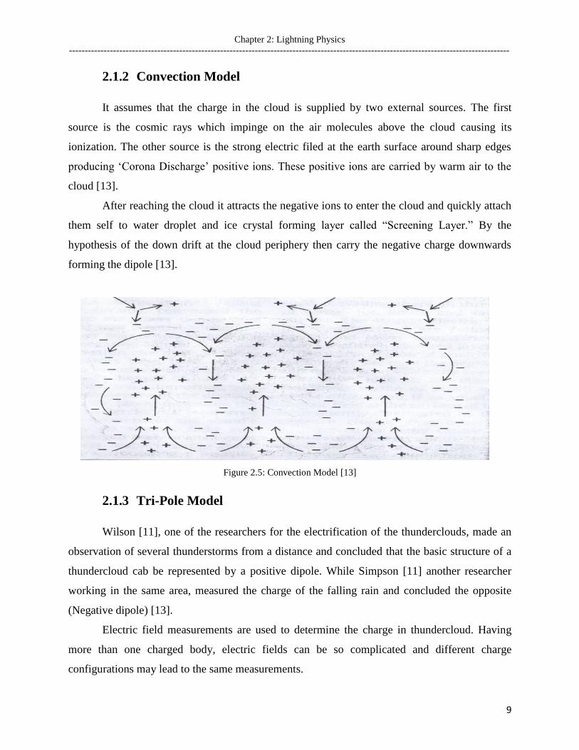
2.1.2 Convection Model
It assumes that the charge in the cloud is supplied by two external sources. The first
source is the cosmic rays which impinge on the air molecules above the cloud causing its
ionization. The other source is the strong electric filed at the earth surface around sharp edges
producing „Corona Discharge‟ positive ions. These positive ions are carried by warm air to the
cloud [13].
After reaching the cloud it attracts the negative ions to enter the cloud and quickly attach
them self to water droplet and ice crystal forming layer called “Screening Layer.” By the
hypothesis of the down drift at the cloud periphery then carry the negative charge downwards
forming the dipole [13].
Figure 2.5: Convection Model [13]
2.1.3 Tri-Pole Model
Wilson [11], one of the researchers for the electrification of the thunderclouds, made an
observation of several thunderstorms from a distance and concluded that the basic structure of a
thundercloud cab be represented by a positive dipole. While Simpson [11] another researcher
working in the same area, measured the charge of the falling rain and concluded the opposite
(Negative dipole) [13].
Electric field measurements are used to determine the charge in thundercloud. Having
more than one charged body, electric fields can be so complicated and different charge
configurations may lead to the same measurements.

Chapter 2: Lightning Physics
--------------------------------------------------------------------------------------------------------------------------------------------
10
Many observations have established that thunderclouds can be modeled as tri-poles, in
which the main region of negative charge is centered between of two positive charges regions
[13].
Although the Convection theory leads more naturally to the tri-pole model, the corona
discharges from sharp edges that produce flux of positive charge toward the base of cloud is not
enough for forming the tri-pole. The perception model can only account for simple dipole.
Several modifications are needed to account for the lower positive charge region and the fact that
rain generally carries positive charge.
Several modifications were proposed, but the final observation that the collision between
ice crystals and grauples particles is dependent on the temperature called charge reversal
temperature. Below this temperature negative charge is transferred to the small particles and vice
versa [13].
Figure 2.6: Charge Reversal Temperature [13]

Chapter 2: Lightning Physics
--------------------------------------------------------------------------------------------------------------------------------------------
11
2.2 Lightning Categories
Lightning can be classified into several categories, but in our work we will mention two
main categories which are the dominant categories:
2.2.1 Cloud-to-cloud
Lightning discharges may occur between areas of cloud having different potentials
without contacting the ground. These are most common between the anvil and lower reaches of a
given thunderstorm. This lightning can sometimes be observed at great distances at night as so-
called "heat lightning". In such instances, the observer may see only a flash of light without
thunder. The "heat" portion of the term is a folk association between locally-experienced warmth
and the distant lightning flashes [11, 12].
Figure 2.7: Different types of lightning
2.2.2 Cloud to earth
Lighting between cloud and earth can be categorized in terms of the direction of motion,
upward or downwards, and the sign of the charge, positive or negative, of the leader that initiate
the discharge Table 2.1 [12].

Chapter 2: Lightning Physics
--------------------------------------------------------------------------------------------------------------------------------------------
12
Table 2.1: Ground Lighting Categories [12]
Negative Cloud to
Ground Lightning
Downward Initiated
Negative Charge
Positive Cloud to
Ground Lightning
Downward Initiated
Positive Charge
Negative Ground to
Cloud Lightning
Upward Initiated
Negative Charge
Positive Ground to
cloud Lightning
Upward Initiated
Positive Charge

Chapter 2: Lightning Physics
--------------------------------------------------------------------------------------------------------------------------------------------
13
Negative cloud to ground is the most common lightning; it accounts for over 90 % of the
world cloud to ground flashes [11, 12].
2.3 Lightning Formation
As a thundercloud having a certain amount of charge moves over an area, an equal but
opposite charge is induced on the earth‟s surface below it, as this charges accumulates more and
more, the air path between the cloud and earth is ionized forming Leader extending downwards.
The negative charged leaders called a "stepped leader“, the stepped leader may branch into a
number of paths as it continues to descend. When a stepped leader approaches the ground, the
presence of opposite charges on the ground enhances the electric field at the ground level,
especially at relative tall structures. When the electric field becomes strong enough at certain
points, a conductive discharge (called a streamer) extends in the upward direction. Then the
lightning strike begins as an extremely large negative electric current (return stroke current)
along the path defined by the return stroke, which has speed of about one third of the speed of
light at the attachment point, but in the opposite direction from ground to cloud [11, 12]. The
whole process is shown in Figure 2.8.
During the strike, successive portions of air become a conductive discharge channel as
the electrons and positive ions of air molecules are pulled away from each other and forced to
flow in opposite directions. The electrical discharge rapidly superheats the discharge channel,
causing the air to expand rapidly and produce a shock wave heard as thunder. The rolling and
gradually dissipating rumble of thunder is caused by the time delay of sound coming from
different portions of a long stroke [11, 12].
A single stroke flash happens when the first return stroke ceases to flow and no more
charge is available to sustain the flash. High speed videos (examined frame-by frame) show that
most lightning strikes are made up of multiple individual strokes. A typical strike is made of 3 to
4 strokes. Successive stokes are usually separated by a relatively large amount of time, typically
40 to 50 milliseconds. Subsequent strokes can cause a noticeable "strobe light" effect. Each
subsequent stroke is preceded by intermediate dart leader, which is usually but weaker than the

Chapter 2: Lightning Physics
--------------------------------------------------------------------------------------------------------------------------------------------
14
initial stepped leader. A subsequent stroke usually re-uses the discharge channel taken by the
previous stroke [11, 12].
Figure 2.8: Lighting Formation Process [12]
The variations in successive discharges are the result of smaller regions of charge within
the cloud being depleted by successive strokes. The sound of thunder from lightning is prolonged
by successive strokes.
2.4 Lightning to Tall Structures
The upward-initiated lightning can occur at mountain tops and at manmade tall
structures, such as towers and sky scrapers. Upward-initiated lightning can be triggered
artificially using rockets trailing conducting wires.
Tall manmade structures are struck by both downward-initiated and upward-initiated
flashes. Upward initiated flashes are branched in the upward direction as shown in Figure 2.9

Chapter 2: Lightning Physics
--------------------------------------------------------------------------------------------------------------------------------------------
15
[14], while downward-initiated flashes are branched downward but are rare to occur at elevated
objects.
The frequency of occurrence of upward-initiated lightning increases with the height of
the structure. For structures smaller or equal 50 meters in height 90% of flashes are downward-
initiated, while for structures higher than 400 meters only 5% of flashes are downward-initiated
[5, 6].
Figure 2.9: Branching of upward-initiated lightning

Chapter 2: Lightning Physics
--------------------------------------------------------------------------------------------------------------------------------------------
16
Many research projects have been conducted with tall man-made structures and the
discovery of upward-initiated lightning is generally attributed to McEachron (1939), who studied
lightning flashes to the Empire State Building in New York City [12]. He observed that most of
the flashes to the Empire State Building are upward-initiated and start at the top of the structure
[17, 18].
After McEachron, many other researchers studied lightning to tall structures including
Berger in Lugano Switzerland on two towers located on Mount San Salvadore [11], Hagenguth
and Anderson at the Empire State Building [12], Garbafnaty at the two 40 m television towers,
one located at Monte Sasso Di Pale and the second located at Monte Rosa [14-18].
In all these studies, it was observed that lightning to tall structures, in the most cases, was
initiated by a leader travelling from the top of the structure towards the cloud. According to
Berger and his measurements, about 85% of lightning flashes were initiated by upward moving
stepped leader. In 1991, studies conducted on CN Tower showed that only 2.8% of the flashes in
that year were downward initiated flashes. Also, studies at the 530 meters high Ostankino
Television tower is Moscow showed that more than 90% of flashes were upward initiated [12].
2.5 CN Tower and Its Lightning Measurement System
The Toronto CN Tower, shown in Figure 2.10 (located at 43.64 N and 79.40 W), was
formerly the world's tallest manmade freestanding structure. It was surpassed in height by the
rising Burj Khalifa, Dubai on 12 September 2007. The work on the tower began in 1973 and
after 40 month of construction, the tower was opened to the public on June 26, 1976 .With a
height of 553 meter and large number of lightning strikes per year, the CN Tower represents an
ideal location for studying the lightning phenomenon. While the flash density in Toronto is about
2 flashes per square kilometer per year, the tower receives tens of strikes each year, for example
in 1991 the tower was hit by 72 flashes [19-21]. Simultaneous measurements of parameters CN
Tower lightning strikes began in 1991. The measurements system can be divided into video
monitoring system, current measurement system and field measurement. There location is shown
in Figure 2.11.

Chapter 2: Lightning Physics
--------------------------------------------------------------------------------------------------------------------------------------------
17
Figure 2.10: CN Tower and its surrounding
The video monitoring system consists of two VHS cameras with 30 frames / sec and
connected to VCRs for recording, one is placed at the Rosebrugh building of the University of
Toronto and the other one at the Ontario Hydro Technology Building. The location of the
cameras provides almost perpendicular views with an angel of 82.5 between them [20]. The
system is used for lighting flash trajectory tracking and also to determine the numbers of strokes

Chapter 2: Lightning Physics
--------------------------------------------------------------------------------------------------------------------------------------------
18
per flash. In some cases the strokes are shorter than the camera resolution that why in 1996 a
high speed camera with 500 frames / sec was installed.
Figure 2.11: CN Tower and the lightning measurement location

Chapter 2: Lightning Physics
--------------------------------------------------------------------------------------------------------------------------------------------
19
The current measurement system located at the CN Tower consists of two Rogowski
coils. A Rogowski coil has the property that its induced voltage is proportional to the time
variation of the net current which represents the current derivative.
The first (old) coil placed at 474 meters AGL (Above Ground Level). It encircles 1/5th
of
the CN Tower‟s steel structure. Assuming a uniform distribution of the current in the azimuth
direction along the CN Tower‟s steels structure, the measured current is estimated to be 20% of
the total current. The 3 meters long coil consists of two 1.5 meters segment, which are
terminated with a resistor at one end (resistor are used to absorb reflections and to damp
oscillations in the coil), and connected to the impedance matching box at the other end. The
impedance matching box is connected to a Sony-Tektronics RTD-710A digitizer through 165
meters of a 50 Ω tri-axial cable. The impedance of the coil seen through the matching box is
made to be 50 Ω, which is the same as the impedance of the tri-axial cable. A schematic of the
coil connection and coil placement at the CN Tower are shown in Figure 2.12.
Figure 2.12: Schematic of old Rogowski coil connection
The second (new) Rogowski coil is placed at 509 meters AGL. It encircles 100% of the
total lightning current. It consists of four, 1.5 meters long segments for a total length of 6 meters.
It is connected to a Sony-Tektronics RTD-710A digitizer through an optical fiber. Two segments
of the coil are connected to the matching box 1 and the other two segments are connected to the

Chapter 2: Lightning Physics
--------------------------------------------------------------------------------------------------------------------------------------------
20
matching box 2. Both boxes are connected to a third matching box to ensure that the impedance
looking into the third box is 50 Ω. A 30 dB attenuator is inserted between the third matching
box and the fiber optical transmitter to limit the output of the new coil to below saturation level.
A schematic of the new Rogowski coil is shown in Figure 2.13.
Figure 2.13: Schematic of new Rogowski coil connection
The data obtained with the new Rogowski coil has considerably better signal-to-noise
ratio (SNR) as compared to data obtained with the old Rogowski coil because the new coil
measure 100% of the total current and it is connected to the digitizer through an optical link.
The field measurement system is allocated at the Rosebrugh building of the University of
Toronto (2.0 km north of the tower). It consists of two field sensors to measure the azimuth
component of the magnetic field and the vertical component of the electric field. The two sensors
are connected to two different channels of the digitizer through coaxial cables. The magnetic

Chapter 2: Lightning Physics
--------------------------------------------------------------------------------------------------------------------------------------------
21
field sensor and the electric field sensor not only measure the fields resulting from the direct
strikes to the tower but also any fields created by the lightning strikes in the vicinity if the tower.
Since the measurement systems are placed at different locations and there is no time
synchronization between them, a Global Positioning System (GPS) has been used. The GPS
represents a master clock to time synchronize all measurements.
2.6 Current Waveform Parameters
Researchers are interested in five major current waveform parameters for lightning
return-stroke studies, namely the current peak, current maximum steepness, risetime to the
current peak (10% level to 90% level of the peak), current pulse width half peak and charge
transferred.
Since the radiated electromagnetic field directly depends on the derivative of the
lightning return-stroke current, the current maximum steepness represents an important
parameter. The current derivative also influences overvoltages caused by lightning striking
power lines and therefore knowledge of maximum steepness is important for protection of tall
structures, power lines as well as static sensitive equipments.
The current peak is taken to be the first peak of the current due to the presence of
another higher peak called the absolute peak. The absolute peak appears due to reflections from
the CN Tower structure discontinuities.
The risetime to the current peak is taken from 10% to 90% of the peak level. This
indicates how fast the signal is. Signals with slow risetime may not have a first peak. This occurs
when reflections arrive before the arrival of the first current peak. In case of currents with low
peaks, it is usually hard to determine the peak due to large SNR.
Figure 2.14 and 2.15 show a CN Tower measured current derivative signal and its
current obtained by numerical integration. The absolute current is also indicated so it can be
compared with the current peak. Other current parameters such as the current pulse width half
peak and charge will be indicated in the later model.

Chapter 2: Lightning Physics
--------------------------------------------------------------------------------------------------------------------------------------------
22
Figure 2.14 Demonstration of current maximum steepness
Figure 2.15: Demonstration of current peak and risetime to the current peak
0 1 2 3 4 5 6 7
-5
0
5
10
15
20
25
30
35
Time (us)
dI/
dt
(kA
/us)
Maximum Steepness
0 1 2 3 4 5 6 7
2
4
6
8
10
12
Time (us)
I (k
A)
Current Peak
Current Rise
Absloute Peak
90 % Current Peak Level
10 % Current Peak Level

Chapter 3: Simulating Functions
----------------------------------------------------------------------------------------------------------------------------- ---------------
23
Chapter 3
Simulating Functions
Different simulating functions have been proposed to model the lightning return-stroke
current using direct measurements preformed at tall structures, such as the CN tower. A suitable
function should fulfill the requirements of the analytical representation of the lightning return-
stroke current [22, 23]:
1. A good approximation to the observed waveshape of the current at the base of the
return stroke channel.
2. Enable the determination of the lightning current waveform parameters:
a. Maximum current
b. Maximum current steepness
c. Risetime to the current peak
d. Current decay time
e. Current pulse width half peak
f. The charge transfer through the channel
3. No discontinuity should appear in first and second derivative especially at the onset
time (t=0).
4. The current function should be differentiable in order to compute the lightning-
generated fields.
5. It should allow the variation of the location of the maximum current steepness.
6. It should be as simple as possible.
In this chapter, four functions will be investigated, namely, the Double Exponential
function, Jones modified Double Exponential function, the Pulse function and Heidler function.
Each of these functions is individually analyzed to:
Check the discontinuity for the current and current derivative at onset
Give initial indication which function best describe the base current of the return
stroke
Chapter 3: Simulating Functions
----------------------------------------------------------------------------------------------------------------------------- ---------------
24
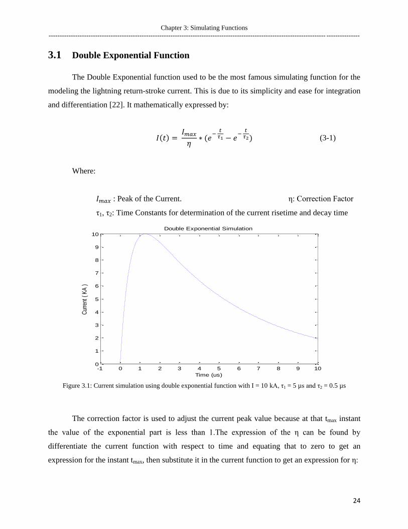
3.1 Double Exponential Function
The Double Exponential function used to be the most famous simulating function for the
modeling the lightning return-stroke current. This is due to its simplicity and ease for integration
and differentiation [22]. It mathematically expressed by:
(3-1)
Where:
: Peak of the Current. η: Correction Factor
τ1, τ2: Time Constants for determination of the current risetime and decay time
Figure 3.1: Current simulation using double exponential function with I = 10 kA, τ1 = 5 µs and τ2 = 0.5 µs
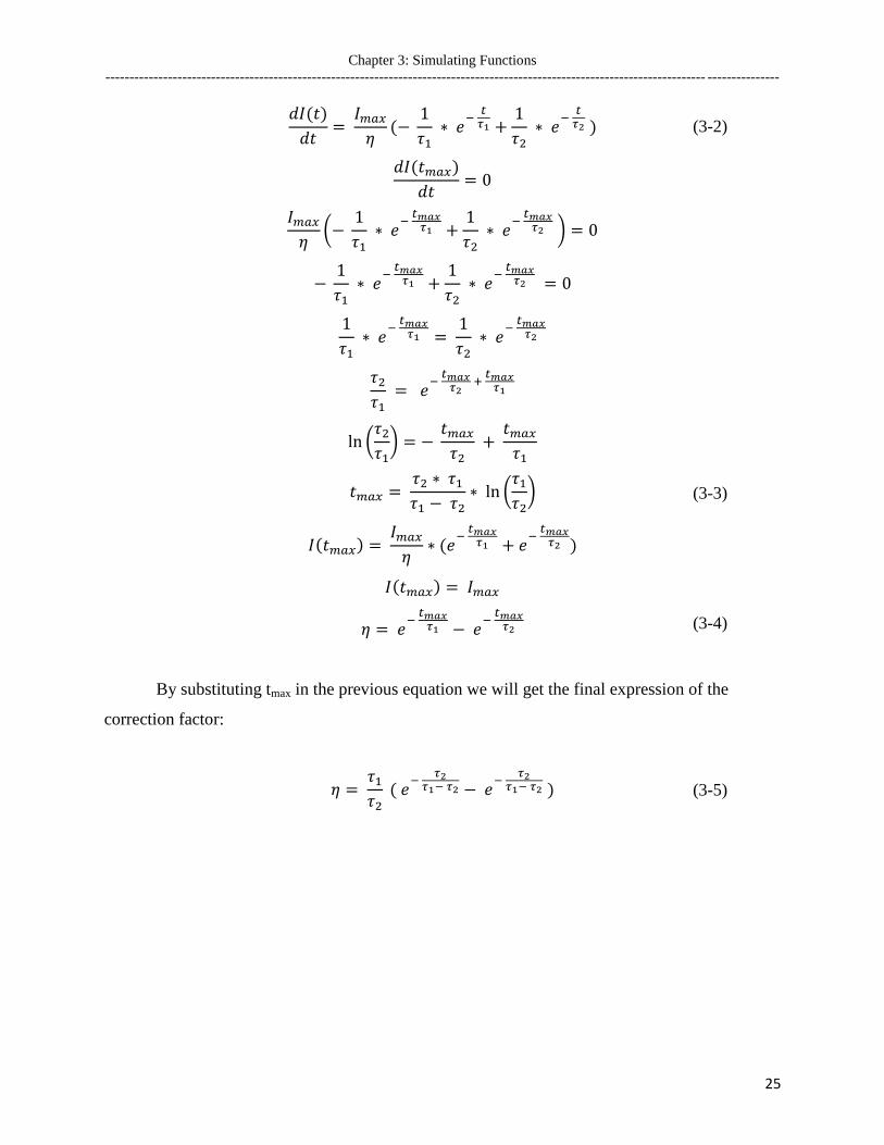
The correction factor is used to adjust the current peak value because at that tmax instant
the value of the exponential part is less than 1.The expression of the η can be found by
differentiate the current function with respect to time and equating that to zero to get an
expression for the instant tmax, then substitute it in the current function to get an expression for η:
-1 0 1 2 3 4 5 6 7 8 9 100
1
2
3
4
5
6
7
8
9
10
Time (us)
Cur
rent
( K
A )
Double Exponential Simulation
Chapter 3: Simulating Functions
----------------------------------------------------------------------------------------------------------------------------- ---------------
25
(3-2)
(3-3)
(3-4)
By substituting tmax in the previous equation we will get the final expression of the
correction factor:
(3-5)

Chapter 3: Simulating Functions
----------------------------------------------------------------------------------------------------------------------------- ---------------
26
Figure 3.2: Current Derivative simulation using Double Exponential Function derivative function with I = 10 kA, τ1
= 5 µs and τ2 = 0.5 µs
The current derivative simulation in Figure 3.2 shows the discontinuity at the onset time t
= 0. The discontinuity value can be calculated as follows:
(3-6)
As shown in Figure 3.2, it is clear to conclude that the maximum steepness value occurs
at the onset time t = 0. In order to derive an expression for the time of occurrence, through which
the current derivative value equals to zero, lets differentiae the Double Exponential function two
times with respect to time and equating it to zero as follows:
(3-7)
-1 0 1 2 3 4 5 6 7 8 9 10-5
0
5
10
15
20
25
30
Time (us)
Cur
rent
Der
ivat
ive
( K
A /
us
)
Double Exponential Derivative Simulation

Chapter 3: Simulating Functions
----------------------------------------------------------------------------------------------------------------------------- ---------------
27
(3-8)
The time of occurrence of the maximum steepness should occur during the rising edge
and before the occurrence of the peak of the current but in the Double Exponential Function that
condition is not satisfied and it occur at the onset time t = 0, in which the time of occurrence of
the second derivative equal to zero at two times of the location of the maximum current which
means the theoretical maximum steepness occurs after the peak of the current.
3.2 Jones Modification
Several modifications have been imposed for the Double Exponential function using
different functions and numerical techniques to eliminate the discontinuity. Time shifting is one
of the imposed modifications. It was introduced by Jones [6]. Figure 3.3 shows the current
simulation. Its mathematically expressed by:
(3-9)
Chapter 3: Simulating Functions
----------------------------------------------------------------------------------------------------------------------------- ---------------
28
Figure 3.3: Current simulation using Jones modification for Double Exponential function with I = 10 kA, τ1 = 5 µs
and τ2 = 0.5 µs
In order to show the effect of the time shifting on the Double Exponential function, let‟s
first find the expression of the correction factor for the modified function. Using the same
method as explained in the Double Exponential function in which time of occurrence of the
maximum current tmax is obtained using the first derivative of the function and then equates it
with zero as follows:
(3-10)
-1 0 1 2 3 4 5 6 7 8 9 100
1
2
3
4
5
6
7
8
9
10
Time (us)
Curr
ent
( K
A )
Jones Modification For Double Exponential Simulation

Chapter 3: Simulating Functions
----------------------------------------------------------------------------------------------------------------------------- ---------------
29
(3-11)
The previous equation does not have general solution to get an expression for
numerical method will be used instead to get the value of . Consequently could be
deduced. Now let‟s investigate the correction factor by substituting in the current
expression (3-9) through which the expression of the correction factor can be obtained:
(3-12)
Since we are concerned with the onset time, then let‟s study the first derivative at t = 0:
(3-13)

Chapter 3: Simulating Functions
----------------------------------------------------------------------------------------------------------------------------- ---------------
30
Figure 3.4: Current Derivative simulation using Double Exponential function derivative function with I = 10 kA, τ1
= 5 µs and τ2 = 0.5 µs
Reduction in the value of the discontinuity at the onset time of the current derivative is
achieved in Jones modification compared with the value of the discontinuity at the onset time of
the current derivative appeared in the Double Exponential function using the same values of the
analytical parameters as shown in Figure 3.5 and 3.6. Also, in Jones‟s modification the
maximum steepness appears during the rising edge and before the occurrence of the maximum
current.
-1 0 1 2 3 4 5 6 7 8 9 10-5
0
5
10
15
20
Time (us)
Cur
rent
Der
ivat
ive
( K
A /
us
)
Jones Modification For Double Exponential Derivative Simulation

Chapter 3: Simulating Functions
----------------------------------------------------------------------------------------------------------------------------- ---------------
31
Figure 3.5: Current simulation using Double Exponential function and Jone modification for Double Exponential
function derivative with I = 10 kA, τ1 = 5 µs and τ2 = 0.5 µs
Figure 3.6: Current Derivative simulation using Double Exponential function and Jone modification for Double
Exponential function derivative with I = 10 kA, τ1 = 5 µs and τ2 = 0.5 µs
-1 0 1 2 3 4 5 6 7 8 9 100
1
2
3
4
5
6
7
8
9
10
Time (us)
Cur
rent
( K
A )
Current Simulation Using Double Exponential and Jones Modfication For Double Exponential
Jones Modification For Double Exponential
Double Exponential
-1 0 1 2 3 4 5 6 7 8 9 10-5
0
5
10
15
20
25
30
Time (us)
Cur
rent
Der
ivat
ive
( K
A /
us
)
Current Derivative Using Double Exponential and Jones Modification For DoubelExponential
Jones Modification For Double Exponential
Double Exponential

Chapter 3: Simulating Functions
----------------------------------------------------------------------------------------------------------------------------- ---------------
32
3.3 Heidler Function
Another set of functions have been proposed to solve the discontinuity It use the idea of
decoupling between the current rise function x(t) and the current decay function y(t), in which at
the current rising function y(t) = 1 and at the current decay function x(t) = 1 .The current
function can be written as :
(3-14)
All of the those functions having same current decay function y(t):
(3-15)
The current rise x(t) can be modeled as:
(3-16)
For t = 0 the current rise will depend on f(t) and g(t) which can be any function,
trigonometric or polynomial, but taking into consideration the elimination of the onset
discontinuity. The exponent n play very important role in decoupling between the rising and
decay current functions when it is value is large, while having low value leading to smooth
change between the both functions. By substituting of both functions in the current function we
get:
(3-17)

Chapter 3: Simulating Functions
----------------------------------------------------------------------------------------------------------------------------- ---------------
33
(3-18)
Where:
For high exponent value n and t < T then A = 1 and B = 0, on the other hand if t > T then
A = 0 and B = 1, so at time t = T A(t) and B(t) behaves like switch or by another word unit step
function. Only a condition should be applied that f(T) = y(T) for smooth changing of the curve at
the switch time.
Although the discontinuity problem could be eliminated by choosing suitable f(t) and g(t)
as stated before but the problem of maximum steepness location cannot vary between 0% to 90%
of the current level, so modification should be applied to overcome such problem or by choosing
different function putting into consideration that no discontinuity should appear. One of those
functions is the power function having the form of:
(3-19)
Where: ki, mi < n
In order to avoid discontinuities at t = 0 ki, mi > 1. Using such function can lead to the
concave shape of current having maximum steepness location approaching 90% of current level.
Considering simple case as following:
(3-20)
It can be shown that the slow rise of current is associated with the low value of n and the
maximum current steepness increases by the increasing of n.

Chapter 3: Simulating Functions
----------------------------------------------------------------------------------------------------------------------------- ---------------
34
Although using the previous simplification of power function would overcome most of
the problems, but a much simpler function have been proposed that can do the job easier. This
function has been proposed by F. Heidler named by Heidler function. Heidler Function is very
frequent used in several standards:
(3-21)
Now let‟s do the same analysis as we did for the Double Exponential function by
deriving the correction factor using of the first derivative:
(3-22)
It is very obvious that the first derivative equals to zero at the onset time t = 0. The
maximum current occurs at tmax having the first derivative of the current equal to zero:

Chapter 3: Simulating Functions
----------------------------------------------------------------------------------------------------------------------------- ---------------
35
And since I(tmax) does not equal zero, then:
(3-23)
In order to get a general expression for tmax we need to solve the previous equation, but
unfortunately there is no general solution for such equation. So instead we will use the iterative
method to get and approximate expression for tmax:

Chapter 3: Simulating Functions
----------------------------------------------------------------------------------------------------------------------------- ---------------
36
(3-24)
Assuming the starting value of tmax = 0:
So the general form of the tmax:
(3-25)
Substituting in the current function to get the correction factor:
(3-26)
To get the exact value of tmax is so complicated so instead a simplification is considered
using the first term only which gives reasonable correction factor value with very small error,
putting into consideration that n > 3 and
> 10. By using that approximation the correction
factor will be:

Chapter 3: Simulating Functions
----------------------------------------------------------------------------------------------------------------------------- ---------------
37
(3-27)
Substituting in the correction factor equation (3-26):
(3-28)
Figure 3.7: Current simulation using Heidler function with I = 10 kA, τ1 = 0.3 µs, τ2 = 3 µs and n = 7
0 0.2 0.4 0.6 0.8 1 1.2 1.4 1.6 1.8 20
1
2
3
4
5
6
7
8
9
10
Time (us)
Cur
rent
( K
A )
Heidler Function Simulation

Chapter 3: Simulating Functions
----------------------------------------------------------------------------------------------------------------------------- ---------------
38
Figure 3.8: Current derivative simulation using Heidler derivative function with I = 10 kA, τ1 = 0.3 µs, τ2 = 3 µs and
n = 7
Starting with the first derivative result, differentiae it one more time with respect to t to
derive the tms:
0 0.2 0.4 0.6 0.8 1 1.2 1.4 1.6 1.8 2-10
0
10
20
30
40
50
60
70
Time (us)
Cur
rent
Der
ivat
ive
( K
A /
us
)
Heidler Function Derivative Simulation

Chapter 3: Simulating Functions
----------------------------------------------------------------------------------------------------------------------------- ---------------
39
(3-29)
It is very obvious to notice that the second derivative equals to zero at the onset time t =
0. This makes the Heidler function suitable to analytical represents the lightning return-stroke
current.
(3-30)
In order to get the general from of the time of occurrence of the maximum steepness,
equation (3-30) should be solved. And since there is no general solution for that equation,
numerical method will be used to get the value for tms. Having the maximum steepness of the
current occurs at the rising edge so the current can be simplified by assuming that decay part of
the current function y(t) = 1:
(3-31)

Chapter 3: Simulating Functions
----------------------------------------------------------------------------------------------------------------------------- ---------------
40
(3-32)
(3-33)

Chapter 3: Simulating Functions
----------------------------------------------------------------------------------------------------------------------------- ---------------
41
(3-34)
Let f1 =
:
By substituting the tms at the approximated current derivative equation (3-32), the value
of the maximum steepness will be:

Chapter 3: Simulating Functions
----------------------------------------------------------------------------------------------------------------------------- ---------------
42
(3-35)
Let f2
:
Now let`s find the value of the current at the time of occurrence of the maximum
steepness:

Chapter 3: Simulating Functions
----------------------------------------------------------------------------------------------------------------------------- ---------------
43
(3-36)
Let f3 =
:
The time of occurrence of the maximum steepness, the value of maximum steepness and
the current value all together depends on the value of k as shown the f1, f2, f3. If n is very large:
(3-37)
(3-38)
Or it can be simply proved by substituting at

Chapter 3: Simulating Functions
----------------------------------------------------------------------------------------------------------------------------- ---------------
44
(3-39)
Although estimating the current maximum steepness was done using an approximation, it
gives an over view about how the and maximum steepness value behaves, also it gives an
indication regarding the dependency between n and time of occurrence of the maximum
steepness and its value.
3.4 Pulse Function
The pulse function is a new function that is used to represent the lightning return-stroke
current [24], and it is mathematically defined by:
(3-40)
Where:
: Maximum Current. η: Correction Factor
τ1, τ2: Time Constants for determination of the current rise and decay time

Chapter 3: Simulating Functions
----------------------------------------------------------------------------------------------------------------------------- ---------------
45
Figure 3.9: Current simulation using Pulse function with I = 10 kA, τ1 = 0.5 µs, τ2 = 10 µs and n = 5
Similar to Heidler function, the correction factor of the pulse can be estimated by using
the first derivative to get the location of the peak of the current tmax and by substituting with the
tmax at the current function (3-40) we get the correction factor.
(3-41)
0 1 2 3 4 5 6 7 8 9 100
1
2
3
4
5
6
7
8
9
10
Time (us)
Curr
ent
( K
A )
Pulse Function Simulation

Chapter 3: Simulating Functions
----------------------------------------------------------------------------------------------------------------------------- ---------------
46
The pulse function does not have discontinuity of the current derivative at the onset time
same as Heilder function.
(3-42)
Substitute with tmax at the current expression (3-40):

Chapter 3: Simulating Functions
----------------------------------------------------------------------------------------------------------------------------- ---------------
47
(3-43)
Figure 3.10: Current derivative simulation using Pulse function derivative with I = 10 kA, τ1 = 0.5 µs, τ2 = 10 µs and
n = 5
0 1 2 3 4 5 6 7 8 9 10-2
0
2
4
6
8
10
Time (us)
Curr
ent
Derivative (
KA
/ u
s )
Pulse Function Derivative Simulation

Chapter 3: Simulating Functions
----------------------------------------------------------------------------------------------------------------------------- ---------------
48
(3-44)
Also we can conclude the second derivative posses no discontinuities at the onset time.
Therefore both functions Heidler and the Pulse satisfies the conditions for analytically
representation of the lightning return-stroke current.

Chapter 3: Simulating Functions
----------------------------------------------------------------------------------------------------------------------------- ---------------
49
(3-45)
Since previous equation (3-45) does not have a general form, the expression of the time
of occurrence of the maximum steepness cannot be estimated. The same approximation
established in Heidler function can be used for the Pulse function, in which the tms occurs at the
rising edge and the decay part of the function can be approximated to y(t) = 1.
(3-46)
(3-47)
(3-48)
(3-49)

Chapter 3: Simulating Functions
----------------------------------------------------------------------------------------------------------------------------- ---------------
50
By substituting the tms at the approximated current derivative equation (3-47), the value
of the maximum steepness will be:
(3-50)
The value of the current at the time of occurrence of the maximum steepness:
(3-51)

Chapter 4: Curve Fitting Technique
----------------------------------------------------------------------------------------------------------------------------- ---------------
51
Chapter 4
Curve Fitting Technique
4.1 Curve Fitting
Data is often given for a discrete value along a continuum. However, estimates may be
required at points between the discrete values or mathematical models may be needed to predict
values that would have been obtained if the experiment had been conducted using larger values
of the independent variables than used in the experiment.
The process of finding a mathematical description that fits a given set of data is known as
“Curve Fitting.” There are two general approaches for curve fitting that are distinguished from
each other on the basis of the amount of error associated with the data.
First, when the data exhibit significant degree of error or noise, in this case the strategy is
to derive a curve that represents a general trend of data. Because any individual data point may
be incorrect there is no need for the line to intersect with these points. An example of this nature
is “Least Square Regression.”
Second, where the data is known to be very precise, the basic approach is to fit a curve or
a series of curves that pass directly through each of the points. The estimation of values between
well-known discrete points is called Interpolation.
In many cases, having a set of data points derived from an experiment where a substantial
error is associated with the data, the second approach (interpolation) is not useful and may yield
to unsatisfactory results when used to estimate the intermediate points or predict further future
points. The lightning return-stroke current measured at the CN Tower is such type of data and
the first approach (Least Square Regression) will be used.

Chapter 4: Curve Fitting Technique
----------------------------------------------------------------------------------------------------------------------------- ---------------
52
4.1.1 Least Square Regression
One strategy for fitting a “best” line through the data would be to minimize the sum of
the residual for all available data, as in:
(4-1)
Where:
n is the total number of points
yi is the y value of data points corresponding to xi
is the value of the model formula evaluated at xi
However, this is an inadequate criterion, as shown in Figure 4.1 which depicts the fit of a
straight line to two points. Obviously the best fit is the line connecting the points. However, any
straight line passing thorough the midpoint of the connecting line results in a minimum value of
equation 4-1.
Figure 4.1: Example of the criteria for “best fit” based on minimizing the sum of the residual

Chapter 4: Curve Fitting Technique
----------------------------------------------------------------------------------------------------------------------------- ---------------
53
Therefore, another logical criterion might be to minimize the sum of the absolute values
of the discrepancies, as in:
(4-2)
Figure 4.2 demonstrates why this criterion is also inadequate. For the four points shown,
any straight line falling within the dashed line will minimize the sum of the absolute values.
Thus, this criterion also does not yield a unique best fit.
Figure 4.2: Example of the criteria for “best fit” based on minimizing the sum of the absolute value of the residual
A third strategy for fitting a best line is the minimax criterion. In this technique, the line
is chosen to minimize the maximum distance that an individual point falls from the line. As
depicted in Figure 4.3, this strategy is illustrated for regression because it gives undue influence
to an outlier, that is, a single point with a large error. It should be noted that the minimax
principle is sometimes well suited for fitting a sample function as well as a complicated function.
A strategy that overcomes the shortcoming of the aforementioned approaches is to
minimize the sum of the squares of the residuals between the measured y and the y calculated.

Chapter 4: Curve Fitting Technique
----------------------------------------------------------------------------------------------------------------------------- ---------------
54
This criterion has a number of advantages, including the fact that it yields a unique
solution for a given set of data.
(4-3)
Figure 4.3: Example of the criteria for “best fit” based on minimizing the maximum error of any individual point
4.1.2 Non Linear Regression
There are many cases in engineering field where nonlinear models must be fitted to the
data. In the present context, these models are defined as those that have a nonlinear dependence
on their parameters. As with linear least square, nonlinear regression is based on determining the
values of the parameters that minimize the sum of the square of the residuals. However, for the
nonlinear case the solution must proceed in an iterative way.
The Gauss-Newton method is one algorithm for minimizing the sum for the squares of
the residual between data and a nonlinear equation. The key concept underlying the technique is
that a Taylor expansion is used to express the original nonlinear equation in an approximate,
linear form. Then, least square theory can be used to obtain new estimates of the parameters that
move in the direction of minimizing the residual.
Chapter 4: Curve Fitting Technique
----------------------------------------------------------------------------------------------------------------------------- ---------------
55
To illustrate how this is done, first the relationship between the nonlinear equation and
the data can be expressed generally as:
(4-4)
Where:
is a function of the independent variable xi and nonlinear function
of the parameters .
is a random error
The nonlinear model can be expanded in a Taylor series around the parameter values and
curtailed after the first derivative:
(4-5)
Where:
j is the initial guess j+1 is the prediction
Thus, the original model is linearized with respect to the parameters and substituting it on
equation 4-4:
(4-6)
It can be reformatted in the matrix form:
(4-7)
Where:

Chapter 4: Curve Fitting Technique
----------------------------------------------------------------------------------------------------------------------------- ---------------
56
is the matrix of partial derivatives of the function evaluated at the guess j.
is the partial derivative of the function with respect to k
th parameter evaluated
at the ith
data point.
D is a vector contains the differences between the measurements and the
function values
contains the changes of the parameter values.
Applying the least square theory on equation 4-7 results in the following normal
equation:
(4-8)
Thus, the approach consists of solving equation 4-8 for , which can be employed to
compute improved values for the parameters, as in:
This procedure is repeated until the solution converges and until it falls below an
acceptable stopping criterion.
(4-9)

Chapter 4: Curve Fitting Technique
----------------------------------------------------------------------------------------------------------------------------- ---------------
57
4.1.3 Quality of Fit
In general, Curve fitting using Least Square Regression is a process of finding a
mathematical model that fits a given set of data points. The term “Model” in this context means a
mathematical formula for a line or curve optimally passes through or near the data points. In
Least Square curve fitting, the condition for the optimal solution is the sum of the squares of the
difference between the model and the data points is minimized.
After fitting the data with one or more models, the comparison between models should be
based on the goodness of the model to the fitted data. There are several ways to investigate the
goodness of the fit. But two methods are commonly used which are visual inspection and
coefficient of determination or R2.
R2 measures how successful the fit is in explaining the variation of the data. It is deifned
as the square of the correlation between the response values and the predicted response values. It
is also called the square of the multiple correlation coefficient and the coefficient of multiple
determination. R2 is defined as the ratio of the sum of squares of the regression (SSR) and the
total sum of squares (SST).
(4-10)
Where:
is the y value predicted by the model for xi
is the mean of the observed data y values
R-square can take on any value between 0 and 1, with a value closer to 1 indicating that a
greater proportion of variance is accounted for by the model. For example, an R-square value of
0.8234 means that the fit explains 82.34% of the total variation in the data about the average.

Chapter 4: Curve Fitting Technique
----------------------------------------------------------------------------------------------------------------------------- ---------------
58
4.2 Modeling Environment
As mentioned before in the previous chapter, there are several functions that can be used
to model lightning return-stroke currents for tall structures, some have major problems because
the discontinuity in the current derivative at the onset time, such as the double exponential
function and its Jones modification. However, other functions like the Pulse and Heidler
functions do not suffer from such problems. This makes the Pulse and Heidler functions
qualified to simulate the lightning return-stroke current.
A comparison between the Pulse and Heilder Functions is to be performed to determine
which function most fit the measured data and can be used to describe the return-stroke current
for tall structure. In order to do such comparison, the first step is to build a modeling
environment for each function individually which can be described as lightning return-stroke
current parameters extraction system for the analytical function. This system which represents an
automated approach for extracting the parameters of the analytical functions is capable to best fit
the function with the measured data. The estimation of the analytical parameters transforms the
discrete data into a continuous signal, from which the current waveform parameters can be
calculated. This parameters extraction system is recognized as a curve fitting system.
Although the measured current signal has been used for simulation, the possibility of
using the measured current derivative signal for simulation is considered. As the current
derivative represents the behavior of how the current changes with time. Any error in the current
usually leads to lager error in the current derivative.
4.2.1 Artificial Digital Signals
The measured data recorded form the CN Tower exhibit some problems:
Noise problem: No electric measurement is free of noise that is why measurement
systems are equipped with different stages of filters. Even the final digitized data
for computerized systems need to have its data filtered.
Reflection problem: This is due to the discontinuities of the structure where the
lightning current flows. The return stroke current will be diluted by reflections,

Chapter 4: Curve Fitting Technique
----------------------------------------------------------------------------------------------------------------------------- ---------------
59
causing the deformation of the measured current. Example: the reflection from the
space deck, the restaurant and the ground base of the CN tower.
The resolution (accuracy) problem: This is a major problem appearing in any
measurement system in any area of research. It can be divided in to two
categories: horizontal time resolution and vertical measured data resolution.
Due to the previous problems, uncertainty exists in the modeling environment of each
function for producing the best results. So this modeling environment needs to be evaluated.
Instead of getting through the measured signal, using artificial signal would be productive to
evaluate the modeling environment through which a comparison between different simulation
functions could be preformed, allowing further development to produce a tool that can be used to
estimate the required current waveform parameters from the measured signal.
The artificial signal can be defined as a signal free of any reflections and noise. It can be
produced the same way as in case of the measured signal in which a signal source producing a
continuous signal then passing through digitizer with digitization rate same as in the measuring
system to produce the artificial signal. The signal source in case of the artificial signal is that
produced by the analytical functions with their analytical parameters being set.
.
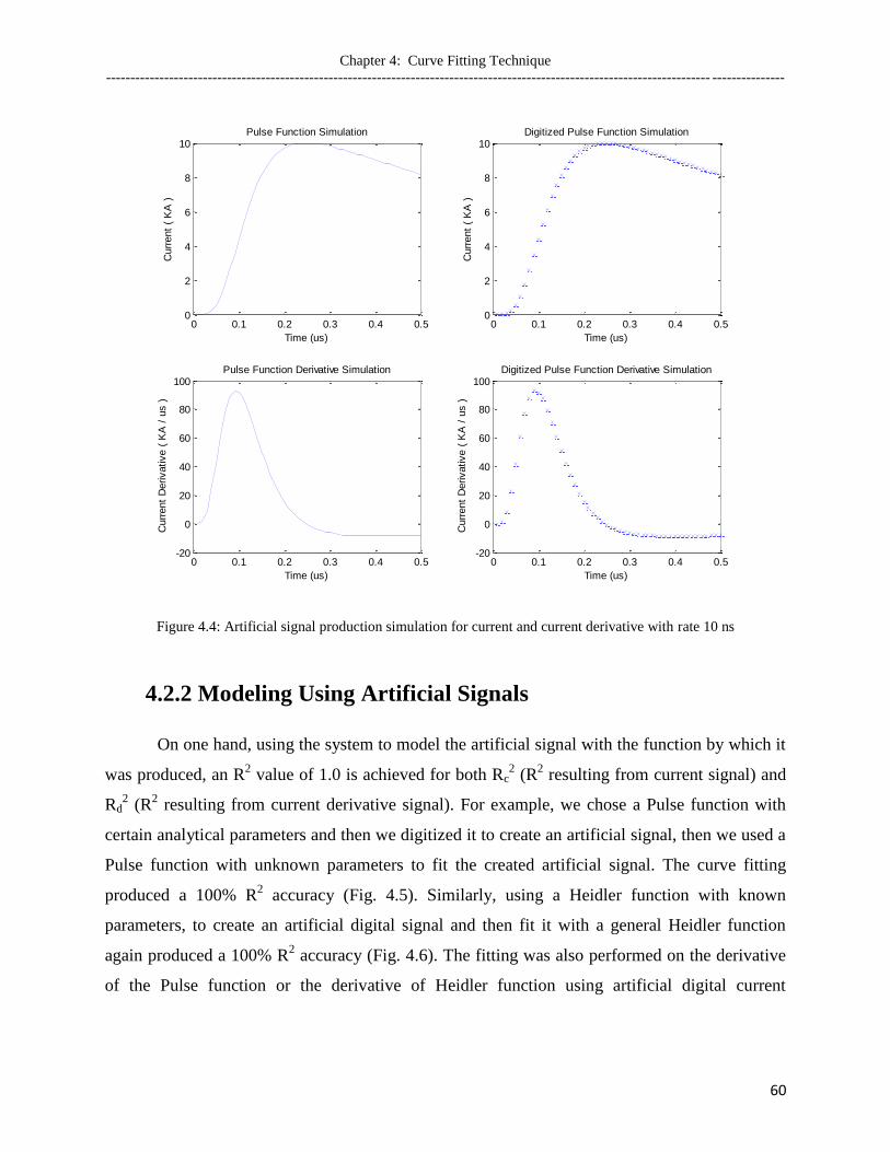
Chapter 4: Curve Fitting Technique
----------------------------------------------------------------------------------------------------------------------------- ---------------
60
Figure 4.4: Artificial signal production simulation for current and current derivative with rate 10 ns
4.2.2 Modeling Using Artificial Signals
On one hand, using the system to model the artificial signal with the function by which it
was produced, an R2 value of 1.0 is achieved for both Rc
2 (R
2 resulting from current signal) and
Rd2 (R
2 resulting from current derivative signal). For example, we chose a Pulse function with
certain analytical parameters and then we digitized it to create an artificial signal, then we used a
Pulse function with unknown parameters to fit the created artificial signal. The curve fitting
produced a 100% R2 accuracy (Fig. 4.5). Similarly, using a Heidler function with known
parameters, to create an artificial digital signal and then fit it with a general Heidler function
again produced a 100% R2 accuracy (Fig. 4.6). The fitting was also performed on the derivative
of the Pulse function or the derivative of Heidler function using artificial digital current
0 0.1 0.2 0.3 0.4 0.50
2
4
6
8
10
Time (us)
Curr
ent
( K
A )
Pulse Function Simulation
0 0.1 0.2 0.3 0.4 0.50
2
4
6
8
10
Time (us)
Curr
ent
( K
A )
Digitized Pulse Function Simulation
0 0.1 0.2 0.3 0.4 0.5-20
0
20
40
60
80
100
Time (us)
Curr
ent
Derivative (
KA
/ u
s )
Pulse Function Derivative Simulation
0 0.1 0.2 0.3 0.4 0.5-20
0
20
40
60
80
100
Time (us)
Curr
ent
Derivative (
KA
/ u
s )
Digitized Pulse Function Derivative Simulation

Chapter 4: Curve Fitting Technique
----------------------------------------------------------------------------------------------------------------------------- ---------------
61
derivative signals (Figs. 4.5 and 4.6). This means that the system was able to retrieve the exact
value of the analytical function parameters from the digitized signal.
Since the artificial signal is formed from the same function being used for fitting and with
condition that the minimum number of points in the signal equal to or greater than the number of
the function unknowns (4 parameters values in each function), then the exact solution can be
obtained. This means the accuracy of the parameters value and the fitting result do not depend on
the number of points in the signal being used or the rate of digitization except the previous
condition is satisfied. Both the Pulse function and Heidler function give the same accuracy in the
result.
Figure 4.5: Curve fitting results using Pulse function artificial signal with I = 10 kA, τ1 = 0.07 µs, τ2 = 1 µs and n =6
0 0.05 0.1 0.15 0.2 0.25 0.3 0.35 0.4 0.45 0.50
5
10
Time ( s )
Curr
ent
( kA
)
0 0.05 0.1 0.15 0.2 0.25 0.3 0.35 0.4 0.45 0.5-50
0
50
100
Time ( s )
Curr
ent
Derivative (
kA
/
s )
Artificial Current (Pulse)
Current Fitting Result
Artificial Derivative Current (Pulse)
Current Derivative Fitting Result

Chapter 4: Curve Fitting Technique
----------------------------------------------------------------------------------------------------------------------------- ---------------
62
Figure 4.6: Curve fitting results using Heidler function artificial signal with I = 10 kA, τ1 = 0.1 µs, τ2 =2 µs and n =5
On the other hand, having the artificial data produced from one function and simulated
using the other function represents a real fitting with artificial signal. Figure 4.7 shows the fitting
of the pulse function to the artificial current signal produced from Heidler function and the
simulation of the corresponding current derivative. It can be concluded that fitting the current
produce better accuracy (Rc2 = 0.9997) than fitting the current derivative (Rd
2 = 0.9954).
0 0.05 0.1 0.15 0.2 0.25 0.3 0.35 0.4 0.45 0.50
5
10
Time ( s )
Curr
ent
( kA
)
0 0.05 0.1 0.15 0.2 0.25 0.3 0.35 0.4 0.45 0.5-50
0
50
100
150
Time ( s )
Curr
ent
Derivative (
kA
/
s )
Artificial Current (Heidler)
Current Fitting Result
Artificial Current Derivative (Heidler)
Current Derivative Fitting Result

Chapter 4: Curve Fitting Technique
----------------------------------------------------------------------------------------------------------------------------- ---------------
63
Figure 4.7: Current fitting results using Pulse current function and the corresponding current derivative simulation
with Heidler artificial signal of parameters I = 10 kA, τ1 = 0.1 µs, τ2 = 2 µs and n = 5
Performing the same fitting technique on the current derivative is shown in Figure 4.8.
The fitting results showed a decrease in comparison with fitting the current (Rc2 = 0.9970 and Rd
2
= 0.9513). It can be recognized from Fig. 4.8 that the fit to the maximum current derivative was
not achieved, which leads to lower current peak.
0 0.05 0.1 0.15 0.2 0.25 0.3 0.35 0.4 0.45 0.50
5
10
Time ( s )
Curr
ent
( kA
)
0 0.05 0.1 0.15 0.2 0.25 0.3 0.35 0.4 0.45 0.5-50
0
50
100
150
Time ( s )
Curr
ent
Derivative (
kA
/
s )
Artificial Current Derivative (Heidler)
Current Derivative Simulation
Artificial Current (Heidler)
Curve Fitting Result

Chapter 4: Curve Fitting Technique
----------------------------------------------------------------------------------------------------------------------------- ---------------
64
Figure 4.8: Current derivative fitting results using Pulse current derivative function and the corresponding current
simulation with Heidler artificial signal of parameters I = 10 kA, τ1 = 0.1 µs, τ2 = 2 µs and n = 5
The current derivative curve fitting results can be improved by setting a better initial
value for each parameter using the values of the parameters obtained from the current fitting.
Figure 4.9, in addition to Rc2 = 0.9993 and Rd
2 = 0.99649, shows the best fit for the current
derivative. Table 1 presents the results of the different fitting approaches of the Pulse function
including fitting of the current, current derivative, current derivative with its parameters being
adjusted along the value of the parameters that is used to set the Heidler function to produce the
artificial signal.
In case of the current derivative fitting with the initial values being adjusted, the error in
the estimated parameters value and the value from current fitting is small. On one hand, this can
be understood as a fine tuning for the results obtained from current fitting. On the other hand, the
current fitting can be used to evaluate the nearest initial values of the parameters for current
derivative fitting. It can be concluded that when fitting the current derivative, the corresponding
current simulation becomes very reasonable and the R-square for the current is high while the
0 0.05 0.1 0.15 0.2 0.25 0.3 0.35 0.4 0.45 0.50
5
10
Time ( s )
Curr
ent
( kA
)
0 0.05 0.1 0.15 0.2 0.25 0.3 0.35 0.4 0.45 0.5-50
0
50
100
150
Time ( s )
Curr
ent
Derivative (
kA
/
s )
Artificial Current Derivative (Heidler)
Current Derrivative Fitting Result
Artificial Current (Heidler)
Current Simulation

Chapter 4: Curve Fitting Technique
----------------------------------------------------------------------------------------------------------------------------- ---------------
65
reverse process is not correct. Also, the pulse function derivative fitting is proved to be very
sensitive to the initial value of its parameters.
Figure 4.9: Current derivative fitting results using Pulse current derivative function and the corresponding current
simulation with Heidler artificial signal of parameters I = 10 kA, τ1 = 0.1 µs, τ2 = 2 µs and n = 5
Table 4.1: Simulation results of the current, current derivative and current derivative with adjusted initial value of
the parameters using the Pulse function
I (kA)
τ1 (µs)
τ2 (µs)
n
Rc
Rd
Heidller (Artificial signal with
10 ns digitization rate)
10
0.1
2
5
------
------
Pulse function current fitting
10.024
0.02892
2.126
20.98
0.99997
0.99537
Pulse function current
derivative fitting
9.6
0.03834
1.729
9.417
0.99702
0.95139
Pulse function current
derivative fitting with current
fitting result initial condition
9.8
0.02835
2.103
23.24
0.99929
0.99649
0 0.05 0.1 0.15 0.2 0.25 0.3 0.35 0.4 0.45 0.50
5
10
Time ( s )
Curr
ent
( kA
)
0 0.05 0.1 0.15 0.2 0.25 0.3 0.35 0.4 0.45 0.5-50
0
50
100
150
Time ( s )
Curr
ent
Derivative (
kA
/
s )
Artificial Current Derivative (Heidler)
Current Derivative Fitting Result
Artificial Current (Heidler)
Current Simulation

Chapter 4: Curve Fitting Technique
----------------------------------------------------------------------------------------------------------------------------- ---------------
66
In case of using the pulse function to produce the artificial signal and Heidler function
represent the fitting function, a similar behavior is obtained. For the current fitting shown in
Figure 4.10, the resultant Rc is 0.9999 and Rd is 0.9946. For the current derivative fitting shown
in Figure 4.11, the resultant Rc is 0.9969 and Rd is 0.9979. The values of the parameters for the
current and current derivative fitting are shown in Table 4.2. On using the analytical parameters
values obtained from the current fitting to set their initial values for the current derivative fitting,
it gives the same result as obtained from the current normal derivative fitting. Heidler function
current derivative fitting is not sensitive to the initial values of the parameters, which makes the
Heidler function derivative fit the signal much easier than using the Pulse function derivative.
Figure 4.10: Current fitting results using Heidler current derivative function and the corresponding current
simulation with Pulse artificial signal of parameters I = 10 kA, τ1 = 0.07 µs, τ2 = 1 µs and n = 6
We can conclude form all the previous simulating results, including the use of the
artificial signals, that the quality of the fit for the simulated current and the current derivative in
case of fitting the current derivative is the best, resulting in highest RD and reasonably high RC.
Also, the Pulse function is found to be very sensitive to the initial point of the parameters while
Heidler function is not for current derivative fitting
0 0.05 0.1 0.15 0.2 0.25 0.3 0.35 0.4 0.45 0.50
5
10
Time ( s )
Curr
ent
( kA
)
0 0.05 0.1 0.15 0.2 0.25 0.3 0.35 0.4 0.45 0.5-50
0
50
100
Time ( s )
Curr
ent
Derivative (
kA
/
s )
Artificial Current Signal (Pulse)
Current Derivative Simulation
Artificial Current Signal (Pulse)
Current Fitting Result

Chapter 4: Curve Fitting Technique
----------------------------------------------------------------------------------------------------------------------------- ---------------
67
Figure 4.11: Current derivative fitting results using Heidler current function and the corresponding current
simulation with Pulse artificial signal of parameters I = 10 kA, τ1 = 0.07 µs, τ2 = 1 µs and n = 6
Table 4.2: Simulation results of the current and current derivative using Heidler function
I (kA)
τ1 (us)
τ2 (us)
n
Rc
Rd
Pulse (Artificial signal
with 10 ns digitization
rate)
10
0.07
1
6
------
------
Heidler function
current fitting
9.98
0.1606
0.9125
3.206
0.9999
0.9946
Heidler function
current derivative
fitting
10.053
0.1593
0.9304
3.168
0.9969
0.9979
0 0.05 0.1 0.15 0.2 0.25 0.3 0.35 0.4 0.45 0.50
5
10
Time ( s )
Curr
ent
( kA
)
0 0.05 0.1 0.15 0.2 0.25 0.3 0.35 0.4 0.45 0.5-50
0
50
100
Time ( s )
Curr
ent
Derivative (
kA
/
s )
Artificial Current Signal (Pulse)
Current Simulation
Artificial Current Signal (Pulse)
Current Derrivative Fitting Result

Chapter 4: Curve Fitting Technique
----------------------------------------------------------------------------------------------------------------------------- ---------------
68
4.3 Initial Conditions
The parameters extraction system is recognized as a curve fitting system. It uses four
analytical function parameters to simulate the measured signal. For any curve fitting technique
the initial value of each parameter and the feasible region where its optimal value exists should
be specified. The more accurate the initial value accompanied by tighter feasible region, the
easier and faster the optimal value can be estimated. In order to do so, it is very important when
looking for the initial value of each parameter to make it independent on the rest of the
parameters as any small error in independent parameters lead to significant error in the
dependant parameters.
As defined in the previous chapter, Heidler function analytical parameters are the same as
those for the Pulse function. These parameters are: Imax, τ1, τ2 and n. The initial value of Imax for
both simulating functions can be estimated using the measured current directly, in which the
peak is its value. The initial value of the rest of the parameters can be deduced using the current
functions for both Heidler and the Pulse functions.
Since the current fitting leads to parameter values very near to the optimal ones, in
addition to its simplicity, the use of the current function is highly recommended for the initial
value search. Also, the approximation by equating the decay part y(t) to unity during the rise
portion produces a separation, which helps in finding the initial values of the parameters τ1 and n
from τ2.
4.3.1 Initial Conditions for the Pulse Function
In case of the Pulse function, we use the approximated current equation 3-46:
Although the value of Imax is known from the measured current and knowing two other
data points is in principal enough for calculating τ1 and n, but for better accuracy three points
will be used to eliminate Imax and η from the equations. The three points should be chosen such
that they occur before the maximum current for the approximation to be applicable.

Chapter 4: Curve Fitting Technique
----------------------------------------------------------------------------------------------------------------------------- ---------------
69
(4-11)
(4-12)
(4-13)
Dividing equation (4-11) over (4-12) to eliminate Imax and η:
(4-14)
The same procedure is done for equation (4-12) and (4-13) to eliminate Imax and η:
(4-15)
Having two equations in two unknowns, simplification is needed to eliminate one of the
parameters. This can be done by taking normal logarithmic for both sides of both equations (4-
14) and (4-15):
(4-16)
(4-17)
Divide (4-16) by (4-17) to eliminate n:

Chapter 4: Curve Fitting Technique
----------------------------------------------------------------------------------------------------------------------------- ---------------
70
(4-18)
Equation (4-18) represents one equation in one unknown τ1. Since it does not have a
general solution for τ1, τ1 can be calculated numerically. Substituting τ1 in equation (4-16), n will
be in the form of:
(4-19)
Using the same procedure for estimating τ2 by applying the original Pulse function
equation (3-40) on two data points where the data points time of occurrence should be after the
peak of the current time of occurrence during the decay portion.
(4-20)
(4-21)
Dividing the previous two equations to eliminate the Imax and η:
(4-22)
Simplify the equation (4-22) to get τ2 in terms of the measured data points and the
calculated other parameters τ1and n:
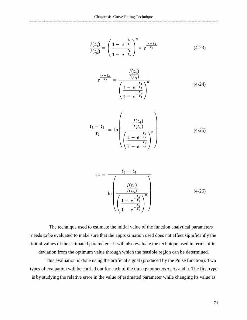
Chapter 4: Curve Fitting Technique
----------------------------------------------------------------------------------------------------------------------------- ---------------
71
(4-23)
(4-24)
(4-25)
(4-26)
The technique used to estimate the initial value of the function analytical parameters
needs to be evaluated to make sure that the approximation used does not affect significantly the
initial values of the estimated parameters. It will also evaluate the technique used in terms of its
deviation from the optimum value through which the feasible region can be determined.
This evaluation is done using the artificial signal (produced by the Pulse function). Two
types of evaluation will be carried out for each of the three parameters τ1, τ2 and n. The first type
is by studying the relative error in the value of estimated parameter while changing its value as

Chapter 4: Curve Fitting Technique
----------------------------------------------------------------------------------------------------------------------------- ---------------
72
shown in Figure 4.12. The second type is by studying the relative error in the value of estimated
parameter while changing the values of the other two parameters as shown in Figures 4.13-4.15.
Figure 4.12: Relative error value for the estimated values of τ1, τ2 and n with the change of its value individually
using the Pulse function initial condition estimation
It can be concluded from the previous figure that the values of the relative error in the
estimation of τ2 are relatively small compared to the relative error in each of τ1 and n. Also, the
values of the relative error due to the estimation of parameters vary proportionally with the
variation of the parameters.
4 6 8 10 12 14 160
0.1
0.2
n
Rela
tive E
rror
% Relative Error of The Estimated n
0.06 0.065 0.07 0.075 0.08 0.085 0.09 0.095 0.1 0.105
0.6
0.8
1
1 ( s )
Rela
tive E
rror
%
Relative Error of The Estimated 1
5 10 15 20 25 300.011
0.012
0.013
2 ( s )
Rela
tive E
rror
%
Relative Error of The Estimated 2

Chapter 4: Curve Fitting Technique
----------------------------------------------------------------------------------------------------------------------------- ---------------
73
Figure 4.13: Relative error value for the estimated values of n with the change of τ1 and τ2 using the Pulse function
initial condition estimation
Figure 4.14: Relative error value for the estimated values of τ2 with the change of τ1 and n using the Pulse function
initial condition estimation
5 10 15 20 25 300.06
0.08
0.1
0.12
0
0.05
0.1
0.15
0.2
0.25
2 ( s )
1 ( s )
Rela
tive E
rror
of
n %
0
5
10
15
0.060.070.080.090.10.11
0
0.05
0.1
0.15
0.2
0.25
n
1 ( s )
Rela
tive E
rror
of
2 %

Chapter 4: Curve Fitting Technique
----------------------------------------------------------------------------------------------------------------------------- ---------------
74
Figure 4.15: Relative error value for the estimated values of τ1 with the change of τ2 and n using the Pulse function
initial condition estimation
For studying the effect of varying τ1and τ2 on the relative error of n, as shown in Figure
4.13, the value of the relative error of n is highly dependent on the changing of τ2 while changing
τ1 does not have significant effect. For studying the effect of varying τ1 and n on the relative
error of τ2, as shown in Figure 4.14, the value of the relative error of τ2 is dependent on the
change in n while changing τ1 does not have any effect. Finally, for studying the effect of
varying n and τ2 on the relative error of τ1, as shown in Figure 4.15, the value of the relative error
of τ1 is dependent on n and highly dependent on τ2.
0
5
10
15
510
1520
2530
0
0.2
0.4
0.6
0.8
1
1.2
1.4
2 ( s )n
Rela
tive E
rror
of
1 %

Chapter 4: Curve Fitting Technique
----------------------------------------------------------------------------------------------------------------------------- ---------------
75
4.3.2 Initial Conditions for Heidler Function
In case of the Heidler function, we use the approximated current equation 3-31:
Although the value of Imax known from the measured current and knowing two other data
points is in principle enough for calculating τ1 and n, but for better accuracy three points will be
used to eliminate Imax and η from the equations:
(4-27)
(4-28)
(4-29)
Divide equation (4-27) by (4-28) to eliminate Imax and η:
(4-30)
Simplify this equation to get single parameter in one side and the other parameters along
with the data on the other side:
(4-31)

Chapter 4: Curve Fitting Technique
----------------------------------------------------------------------------------------------------------------------------- ---------------
76
(4-32)
(4-33)
(4-34)
(4-35)
The separation between the τ1 and n is achieved in equation (4-35). The same technique
carried out, divide equation (4-28) by (4-29) and simplify to get the second equation of τ1 and n:
(4-36)
Having two equations in two unknowns, simplification is needed to eliminate one of the
parameters. This can be done by taking normal logarithmic for both sides of both equations (4-
35) and (4-36) then dived both equations to eliminate n:
(4-37)
Simplify the previous equation:
(4-38)

Chapter 4: Curve Fitting Technique
----------------------------------------------------------------------------------------------------------------------------- ---------------
77
(4-39)
(4-40)
The previous equation represents one equation with one unknown n. Since it does not
have a general solution for n, n can be calculated numerically. Substituting in the n on of the
previous equation, τ1 will be in the form of:
(4-41)
Using the same procedure for finding τ2 by applying the original current Heidler function
equation (3-21) on two data points where the data points time of occurrence should be after the
peak current time of occurrence during the decay portion.
(4-42)
(4-43)
Dividing the two equations to eliminate the Imax and η:

Chapter 4: Curve Fitting Technique
----------------------------------------------------------------------------------------------------------------------------- ---------------
78
(4-44)
Simplify the previous equation to get τ2 in terms of the measured data points and the
calculated other parameters τ1and n:
(4-45)
(4-46)
(4-47)
(4-48)
The evaluation is done using the artificial signal (Produced by Heidler function). The
same two types of evaluation done for the initial value of the analytical parameters of the Pulse
function will be repeated for the analytical parameters of Heidler function. The first type results
are shown in Figure 4.16. The second type results are shown in Figures 4.17, 4.18 and 4.19.

Chapter 4: Curve Fitting Technique
----------------------------------------------------------------------------------------------------------------------------- ---------------
79
Figure 4.16: Relative error value for the estimated values of τ1, τ2 and n with the change of its value individually
using Heidler function initial condition estimation
It can be concluded from the previous figure that the values of the relative error in
estimation of τ2 are negligible. It is clear that the relative error due to the estimation of n is
inversely proportional with the change in n, while the relative error due to the estimation of τ1 is
directly proportional with the change in τ1. However, the relative error in τ2 follows a non
uniform behavior with the change in τ2.
2 4 6 8 10 12 14 160
0.1
0.2
n
Rela
tive E
rror
% Relative Error of The Estimated n
0 0.1 0.2 0.3 0.4 0.5 0.6 0.7 0.8 0.9 10
1
2
1 ( s )
Rela
tive E
rror
%
Relative Error of The Estimated 1
5 10 15 20 25 306
6.5
7x 10
-5
2 ( s )
Rela
tive E
rror
%
Relative Error of The Estimated 2

Chapter 4: Curve Fitting Technique
----------------------------------------------------------------------------------------------------------------------------- ---------------
80
Figure 4.17: Relative error value for the estimated values of n with the change of τ1 and τ2 using Heidler function
initial condition estimation
Figure 4.18: Relative error value for the estimated values of τ2 with the change of τ1 and n using Heidler function
initial condition estimation
510
1520
2530
0
0.5
10
0.5
1
1.5
2 ( s )
1 ( s )
Rela
tive E
rror
of
n %
2 4 6 8 10 12 14 160
0.5
1
-0.5
0
0.5
1
1.5
2
2.5
3
3.5
1 ( s )
n
Rela
tive E
rror
of
2 %

Chapter 4: Curve Fitting Technique
----------------------------------------------------------------------------------------------------------------------------- ---------------
81
Figure 4.19: Relative error value for the estimated values of τ1 with the change of τ2 and n using Heidler function
initial condition estimation
For studying the effect of varying τ1and τ2 on the relative error of n, as shown in Figure
4.17, the value of the relative error of n is inversely proportional to the change of τ2 while
directly proportional with the change of τ1. For studying the effect of varying τ1 and n on the
relative error of τ2, as shown in Figure 4.18, the value of the relative error of τ2 is directly
proportional with high values of τ1 and inversely proportional to low values of n and is constant
otherwise. Finally, In the case of studying the effect of varying n and τ2 on the relative error of τ1
as shown in Figure 4.19, the value of the relative error of τ1 is inversely proportional to the
change in both n and τ2.
It is very clear that the relative error value for the estimated initial value of the parameters
is very small and acceptable for both functions. Also the effect of changing other parameters on
the relative error of the initial value of the estimated parameter vanishes as the parameters value
increases. In general the approximation used to estimate the initial values of the parameters is
acceptable.
0
5
10
155 10 15 20 25 30
0
0.2
0.4
0.6
0.8
2 ( s )
n
Rela
tive E
rror
of
1 %

Chapter 5: Results & Discussions
----------------------------------------------------------------------------------------------------------------------------- ---------------
82
Chapter 5
Results & Discussions
In Chapter 4, the initial value estimation of the analytical parameters of the functions and
the idea of using the artificial digital signals for evaluating the analytical parameters estimation
system were discussed. The evaluation of the initial value estimation process has proved the
success of the used method and showed how near the initial values of the analytical parameters is
with respect to the optimal ones. Since the initial value estimation process resulted in analytical
parameters values very near to the optimal one and the least square technique is used to concise
this value to the optimal, then the system can be applied on the measured signal.
As discussed before, the measured signal has some problems, but the major ones are the
reflections due to the discontinuities in the tower structure and the limited duration of the
measured signal, is less than the duration of the full signal. Previously, researches used to study
only the first impulse of the measured current derivative signal just before the current peak, as
shown in Figure 5.1, before the arrival of reflections in the measured signal. The first current
derivative impulse represents the rising edge of the current waveform. This led to some
limitations in calculating the current waveform parameters, specially the decay time, the current
pulse width at half peak level and the charge. In order to calculate all the current waveform
parameters, the fitting function should fit the first impulse of the derivative and should have the
same decay behavior as in the measured current signal.

Chapter 5: Results & Discussions
----------------------------------------------------------------------------------------------------------------------------- ---------------
83
Figure 5.1: First impulse of the measured signal
Due to the existence of the mentioned problems, it is necessary when judging the quality
of the fit to use some guidelines along with R2. These guidelines are the maximum steepness
time of occurrence, zero crossing time of the current derivative and the peak value of the current
waveform. Applying the initial value estimation for the analytical parameters along with the least
square curve fitting method and using both functions as simulating functions, keeping in mind
the guidelines and R2 for judging the quality of the fit, the comparison between the Pulse
function and Heidler function can be performed on fitting the current derivative signal measured
at the CN Tower through which the current waveform parameters can be calculated.
A complete analysis is carried out for each function individually to understand its
behavior while fitting the measured signal. The effect of the reflections on the fitting process has
been investigated while applying a set of conditions on the fitting process until the best fitting is
achieved. The last step after achieving the best fitting for each function is the comparison to
determine which one fits better the CN Tower measured signal, and then use the better function
to calculate the current waveform parameters.
0 0.5 1 1.5 2 2.5 3 3.5 4 4.5 5-5
0
5
10
15
Time (s)
Curr
ent
(kA
)
0 0.5 1 1.5 2 2.5 3 3.5 4 4.5 5-20
0
20
40
Time (s)
Curr
ent
Derivative (
kA
/
s)
First Impulse
First Impulse

Chapter 5: Results & Discussions
----------------------------------------------------------------------------------------------------------------------------- ---------------
84
Figures 5.2 and 5.3 show the result of applying the derivative of the Pulse and Heidler
functions to fit the current derivative measured signal at the CN Tower and the simulation of the
corresponding current with the integration of the measured signal. The initial values of the
analytical parameters, the values of the analytical parameters after the fitting process and the
corresponding R2 are listed in Table 5.1. It is clear that the initial values of Imax, τ1 and n are far
from the final values.
Using the curve fitting process, it is very clear that the maximum steepness value and
time of occurrence have not been achieved, the zero crossing is shifted away which leads to
wrong risetime value. Consequently the guidelines for judging the quality of the fit were not
fulfilled. Also the decay of the fitted signal is very slow with respect to the measured signal
which leads to very large decay time and charge on calculating from the fitting functions. As a
result, the fitting process needs to be improved for both functions.
Figure 5.2: Fitting results of the Pulse and Heidler functions for the measured current derivative signal and the corresponding
current
0 5 10 15 20 25 30 35 40 45 50-5
0
5
10
15
Time (s)
Curr
ent
(kA
)
0 5 10 15 20 25 30 35 40 45 50-20
0
20
40
Time (s)
Curr
ent
Derivative (
kA
/
s)
Pulse Derivative
Heidler Derivative
Measured Current Derivative Signal
Pulse Function
Heidler Function
Current Signal
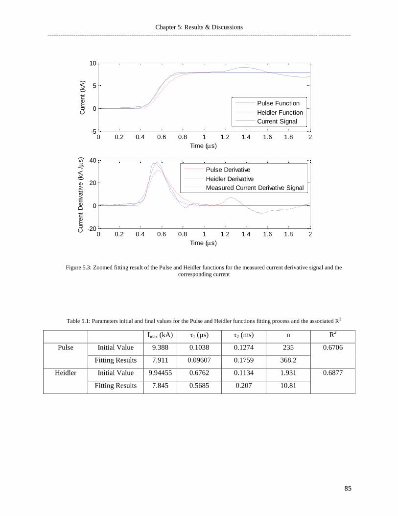
Chapter 5: Results & Discussions
----------------------------------------------------------------------------------------------------------------------------- ---------------
85
Figure 5.3: Zoomed fitting result of the Pulse and Heidler functions for the measured current derivative signal and the
corresponding current
Table 5.1: Parameters initial and final values for the Pulse and Heidler functions fitting process and the associated R2
Imax (kA) τ1 (µs) τ2 (ms) n R2
Pulse Initial Value 9.388 0.1038 0.1274 235 0.6706
Fitting Results 7.911 0.09607 0.1759 368.2
Heidler Initial Value 9.94455 0.6762 0.1134 1.931 0.6877
Fitting Results 7.845 0.5685 0.207 10.81
0 0.2 0.4 0.6 0.8 1 1.2 1.4 1.6 1.8 2-5
0
5
10
Time (s)
Curr
ent
(kA
)
0 0.2 0.4 0.6 0.8 1 1.2 1.4 1.6 1.8 2-20
0
20
40
Time (s)
Curr
ent
Derivative (
kA
/
s)
Pulse Derivative
Heidler Derivative
Measured Current Derivative Signal
Pulse Function
Heidler Function
Current Signal

Chapter 5: Results & Discussions
----------------------------------------------------------------------------------------------------------------------------- ---------------
86
5.1 Estimating τ2
As explained in Chapter 3, the structure of Heidler function and the Pulse function is
divided into current rise portion x(t) and current decay portion y(t) as in equation (3-14). By
studying the effect of the rise portion x(t) for both functions when t >> τ1, during the decay of the
signal, the functions seem to be insensitive to the rise portion (x(t) ≈ 1). For further investigation,
Figure 5.4 shows the simulation of the rising portion of the function using parameters values
from Table 4.2. It is very clear that the rising portion of the function saturates just after reaching
the peak of the current. It reaches 99% of the maximum value at 0.6 µs for the Pulse function and
at 0.65 µs for Heidler function. In this case the decay portion of the function will be the
dominating part.
Figure 5.4: Fitting the rising portion of the Pulse and Heidler functions
0 5 10 15 20 25 30 35 40 45 500
5
10
15
Time (s)
Curr
ent
(kA
)
0 0.5 1 1.50
5
10
15
Time (s)
Curr
ent
(kA
)
Pulse Function (Rise portion)
Heidler Function (Rise portion)
Pulse Function (Rise portion)
Heidler Function (Rise portion)
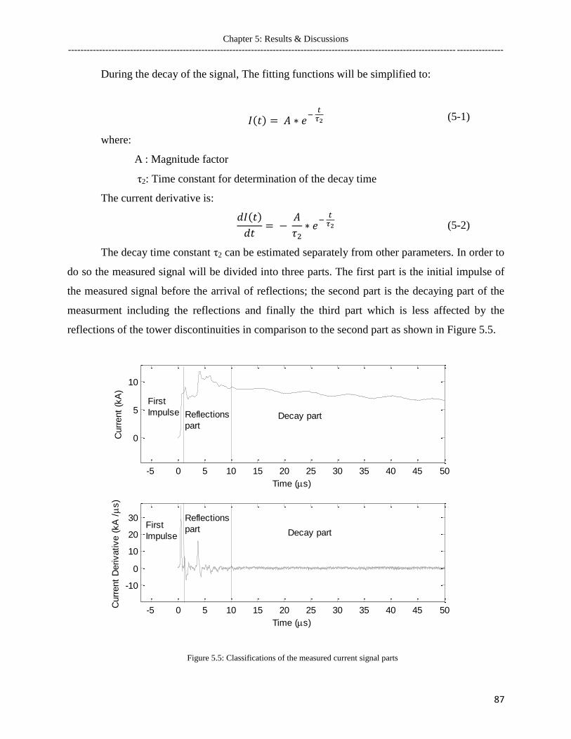
Chapter 5: Results & Discussions
----------------------------------------------------------------------------------------------------------------------------- ---------------
87
During the decay of the signal, The fitting functions will be simplified to:
(5-1)
where:
A : Magnitude factor
τ2: Time constant for determination of the decay time
The current derivative is:
(5-2)
The decay time constant τ2 can be estimated separately from other parameters. In order to
do so the measured signal will be divided into three parts. The first part is the initial impulse of
the measured signal before the arrival of reflections; the second part is the decaying part of the
measurment including the reflections and finally the third part which is less affected by the
reflections of the tower discontinuities in comparison to the second part as shown in Figure 5.5.
Figure 5.5: Classifications of the measured current signal parts
-5 0 5 10 15 20 25 30 35 40 45 50
0
5
10
Time (s)
Curr
ent
(kA
)
-5 0 5 10 15 20 25 30 35 40 45 50
-10
0
10
20
30
Time (s)
Curr
ent
Derivative (
kA
/
s)
Decay part
Decay part
Reflections
part
First
Impulse
Reflections
partFirst
Impulse

Chapter 5: Results & Discussions
----------------------------------------------------------------------------------------------------------------------------- ---------------
88
The current derivative measured signal contains high frequency noise, which results in
the failure of estimating τ2 from the current derivative directly. Therefore, we use the current,
which is the integration of the measured current derivative signal, for the estimation of τ2. The
process of integrating the current derivative signal filters the high frequency noise without
affecting the decay behavior of the current. Using this method to estimate τ2 reduces the
unknown analytical parameters of the function to three, namely τ1, n and Imax.
Applying the curve fitting process on the decay part of the signal using the fitting
function of equation (5-1), A and τ2 can be estimated. Figure 5.6 shows the result of the fitting
process with τ2 value of 0.1239 ms and A value of 9.72 kA. The magnitude factor A is not
important because its value is affected by the reflection while τ2 represents the decay behavior of
the current, which is the integration of the measured signal.
Figure 5.6: Simulation of the fitting result of the Pulse and Heidler functions on the integration of the measured signal decay
part (current decay part)
The rest of the parameters can be estimated by applying the simulating functions on the
first impulse of the current derivative as shown in Figures 5.7 and 5.8. The decay part for both
0 5 10 15 20 25 30 35 40 45 506
6.5
7
7.5
8
8.5
9
9.5
10
Time (s)
Curr
ent
(kA
)
Decay part of the measured signal Integration (Current)
Current fitting of the decay part

Chapter 5: Results & Discussions
----------------------------------------------------------------------------------------------------------------------------- ---------------
89
functions has been substantially improved. For the Pulse function, the current derivative fitting is
acceptable but the corresponding current has lower values, the peak current is not achieved and
its time of occurrence is shifted. For Heidler function, although the current derivative fitting is
not as good as the Pulse function but the corresponding current is much better than that of the
Pulse function. The problem in Heidler function fitting is that the value of the peak current and
its time of occurrence have not been simultaneously achieved.
Table 5.2 contains the initial value of the analytical parameters and the value of the
analytical parameters after the fitting process and the corresponding R2. It is very important to
note that the value of τ2 is fixed before and after the fitting process of the first impulse as it was
obtained from the corresponding decay part of the signal. Using the value of τ2 in the estimation
of the initial value of other analytical parameters initial value yields very accurate initial values
for τ1 and Imax, close to the optimal one.
Figure 5.7: Simulation of fitting result of the Pulse and Heidler functions for the measured current derivative signal with
fixed τ2 and the corresponding current signal
0 5 10 15 20 25 30 35 40 45 50-5
0
5
10
15
Time (s)
Curr
ent
(kA
)
0 5 10 15 20 25 30 35 40 45 50-20
0
20
40
Time (s)
Curr
ent
Derivative (
kA
/
s)
Pulse Derivative
Heidler Derivative
Measured Current Derivative Signal
Pulse Function
Heidler Function
Current Signal

Chapter 5: Results & Discussions
----------------------------------------------------------------------------------------------------------------------------- ---------------
90
Figure 5.8: Zoomed simulation of fitting result of the Pulse and Heidler functions for the measured current derivative signal
with fixed τ2 and the corresponding current signal
Table 5.2: Parameters‟ initial and final values for the Pulse and Heidler functions fitting process with fixed τ2 and the
associated R2
Imax (kA) τ1 (µs) τ2 (ms) n R2
Pulse Initial Value 7.6 0.07679 0.1239 876.3 0.9006
Fitting Results 7.5 0.07775 0.1239 1108
Heidler Initial Value 7.586 0.559 0.1239 11.54 0.8963
Fitting Results 7.667 0.5684 0.1239 10.83
0 0.2 0.4 0.6 0.8 1 1.2 1.4 1.6 1.8 2-5
0
5
10
Time (s)
Curr
ent
(kA
)
0 0.2 0.4 0.6 0.8 1 1.2 1.4 1.6 1.8 2-20
0
20
40
Time (s)
Curr
ent
Derivative (
kA
/
s)
Pulse Derivative
Heidler Derivative
Measured Current Derivative Signal
Pulse Function
Heidler Function
Current Signal
Chapter 5: Results & Discussions
----------------------------------------------------------------------------------------------------------------------------- ---------------
91
5.2 Estimating Imax
Since the value of the peak of the current is a common problem, it can be adjusted by
forcing the value of the peak of the current Imax to have a certain value. This value can be
estimated by visual investigation of the integration of the measured current derivative signal. By
assigning the value of Imax, the number of analytical parameters will be reduced to two: n and τ1.
Using the value of τ2, previously obtained, and assigning to Imax its measured value (7.9
kA), and applying the curve fitting process on the first impulse, the other analytical parameters
can easily estimated. As shown in Figure 5.9, although the Pulse function current improves, the
maximum steepness value and its time of occurrence, as well as the zero crossing of the current
derivative need to be improved to best fit the measured signal. Heidler function shows the same
problems as the Pulse function.
The values of the analytical parameters, before and after the fitting process and the
corresponding R2 are listed in Table 5.3. Imax and τ2 values are the same as the fitting process
involved on n and τ1. It is very clear that R2 of both functions is reduced slightly but the current
simulation is improved.

Chapter 5: Results & Discussions
----------------------------------------------------------------------------------------------------------------------------- ---------------
92
Figure 5.9: Zoomed simulation of fitting result of the Pulse and Heidler functions for the measured current derivative signal
with fixed τ2 and Imax and the corresponding current signal
Table 5.3: Parameters‟ initial and final values for the Pulse and Heidler functions fitting process with fixed τ2 and Imax and the
associated R2
Imax (kA) τ1 (µs) τ2 (ms) n R2
Pulse Initial Value 7.9 0.06962 0.1239 1410 0.8986
Fitting Results 7.9 0.0773 0.1239 1166
Heidler Initial Value 7.9 0.5611 0.1239 14.44 0.8959
Fitting Results 7.9 0.5689 0.1239 10.6
0 0.2 0.4 0.6 0.8 1 1.2 1.4 1.6 1.8 2-5
0
5
10
Time (s)
Curr
ent
(kA
)
0 0.2 0.4 0.6 0.8 1 1.2 1.4 1.6 1.8 2-20
0
20
40
Time (s)
Curr
ent
Derivative (
kA
/
s)
Pulse Function
Heidler Function
Current Signal
Pulse Derivative
Heidler Derivative
Measured Current Derivative Signal

Chapter 5: Results & Discussions
----------------------------------------------------------------------------------------------------------------------------- ---------------
93
5.3 Applying Constraints
Another way for improving the fitting process is by introducing a constraint to force the
analytical parameters to reach their optimal values. This constraint is applied by adjusting either
the time of occurrence of the zero crossing of the current derivative or the time of occurrence of
the maximum steepness of the current to its measured value. The analytical analysis preformed
in chapter 3 can be used to define the suitable constraints for each function. We refer to these
constraints as time-forcing constraints.
Using the known values of τ2 and Imax, which were previously estimated, τ1 can be
expressed in terms of n or vice versa. Accordingly, the number of analytical parameters of the
functions will be reduced to one.
5.3.1 Condition of Current Derivative Zero Crossing
Firstly, the time-forcing constraint will be applied to adjust the zero crossing of the
current derivative to its measured value. For the Pulse function, applying the constraint using
equation (3-42), n can be expressed in terms of τ1:
(5-3)
By substituting n in the Pulse function equation (3-40) and its derivative, equation (3-41),
the only unknown analytical parameter will be τ1. The function and its derivative can be
reformatted as follows:
(5-4)

Chapter 5: Results & Discussions
----------------------------------------------------------------------------------------------------------------------------- ---------------
94
(5-5)
For Heidler function, applying the constraint using equation (3-27), τ1 can be expressed
in terms of n:
(5-6)
By substituting n in Heidler function equation (3-21) and its derivative equation (3-22),
the only unknown analytical parameter will be n. The function and its derivative can be
reformatted as follows:
(5-7)
(5-8)
The equations of the simulating functions (5-5) and (5-8), representing the Pulse and
Heidler functions after using the time forcing constraint for the zero crossing, respectively, are
applied on the measured current derivative first impulse to find the optimal value of τ1 or n. An
overshoot for the maximum steepness value of the current signal occurred leading to a very fast
rise in the current signal as shown in Figure 5.10. Consequently the zero crossing constraint was
not possible to apply to achieve the optimal value of the analytical parameters.

Chapter 5: Results & Discussions
----------------------------------------------------------------------------------------------------------------------------- ---------------
95
The resultant R2 value of the fitting process is very poor and proves that such condition
causes the analytical parameters to deviate from their optimal values. The initial values of the
analytical parameters, values of the parameters after the fitting process and the corresponding R2
are listed in Table 5.4.
Figure 5.10: Zoomed simulation of fitting result of the Pulse and Heidler functions for the measured current derivative signal
with fixed τ2, Imax and with forcing time constraints of the zero crossing of the current derivative signal and the corresponding
current signal
Table 5.4: Parameters‟ initial and final values for the Pulse and Heidler functions fitting process with fixed τ2, Imax and with
forcing time constraints of the zero crossing of the current derivative signal and the associated R2
Imax (kA) τ1 (µs) τ2 (ms) n R2
Pulse Initial Value 7.9 0.02476 0.1239 ------------- 0.216
Fitting Results 7.9 0.03476 0.1239 -------------
Heidler Initial Value 7.9 ------------- 0.1239 22.81 0.4424
Fitting Results 7.9 ------------- 0.1239 20.38
0 0.2 0.4 0.6 0.8 1 1.2 1.4 1.6 1.8 2-5
0
5
10
Time (s)
Curr
ent
(kA
)
0 0.2 0.4 0.6 0.8 1 1.2 1.4 1.6 1.8 2-50
0
50
100
Time (s)
Curr
ent
Derivative (
kA
/
s)
Pulse Function
Heidler Function
Current Signal
Pulse Derivative
Heidler Derivative
Measured Current Derivative Signal

Chapter 5: Results & Discussions
----------------------------------------------------------------------------------------------------------------------------- ---------------
96
5.3.2 Time of Maximum Steepness Condition
Secondly, the time-forcing constraint will be applied to adjust the time of occurrence of
the maximum steepness of the current signal to its measured value. For the Pulse function,
applying the constraint using equation (3-49), n can be expressed in terms of τ1:
(5-9)
By substituting n in the Pulse function equation (3-40) and its derivative equation (3-41),
the only unknown parameter will be τ1. The function and its derivative can be reformatted as
follows:
(5-10)
(5-11)
Similarly, for Heidler function, applying this constraint using equation (3-34), τ1 can be
expressed in terms of n:
(5-12)
By substituting n in Heidler function equation (3-21) and its derivative equation (3-22),
the only unknown parameter will be n. The function and its derivative can be reformatted as
follows:

Chapter 5: Results & Discussions
----------------------------------------------------------------------------------------------------------------------------- ---------------
97
(5-13)
(5-14)
Equations (5-11) and (5-14) representing the Pulse and Heidler functions after using the
time-forcing constraint for the time of occurrence of the maximum steepness, respectively, are
applied on the measured current derivative first impulse to find the optimal value of τ1 or n. The
best fit is achieved for both functions as shown in Figure 5.11.
Table 5.5 contains the initial values of the analytical parameters, the values of the
analytical parameters after the fitting process and the associated R2 of the fitting process. The
Pulse function followed the guidelines and the highest R2 value supported this guidelines. It is
very clear that the Pulse function better fits the measured current derivative and it also better
simulates the current signal than those of Heidler function.

Chapter 5: Results & Discussions
----------------------------------------------------------------------------------------------------------------------------- ---------------
98
Figure 5.11: Zoomed simulation of fitting result of the Pulse and Heidler functions for the measured current derivative signal
with fixed τ2, Imax and with forcing time constraints of the maximum steepness of current signal and the corresponding
current signal
Table 5.5: Parameters‟ initial and final values for the Pulse and Heidler functions fitting process with fixed τ2, Imax and with
forcing time constraints of the the maximum steepness of current signal and the associated R2
Imax (kA) τ1 (µs) τ2 (ms) n R2
Pulse Initial Value 7.9 0.05181 0.1239 ------------- 0.8771
Fitting Results 7.9 0.07797 0.1239 -------------
Heidler Initial Value 7.9 ------------- 0.1239 12.36 0.8371
Fitting Results 7.9 ------------- 0.1239 9.629
0 0.2 0.4 0.6 0.8 1 1.2 1.4 1.6 1.8 2-5
0
5
10
Time (s)
Curr
ent
(kA
)
0 0.2 0.4 0.6 0.8 1 1.2 1.4 1.6 1.8 2-20
0
20
40
Time (s)
Curr
ent
Derivative (
kA
/
s)
Pulse Function
Heidler Function
Current Signal
Pulse Derivative
Heidler Derivative
Measured Current Derivative Signal

Chapter 5: Results & Discussions
----------------------------------------------------------------------------------------------------------------------------- ---------------
99
5.4 Current Waveform Parameters
The described fitting process represents the best method to reach the optimal fit for
simulating the measured signal. The objective is not only simulating the full measured signal
including the decay part but also calculating all current waveform parameters. Using this fitting
process for the Pulse function, all current waveform parameters can be calculated, which leads to
the establishment of extensive cumulative statistics regarding each waveform parameter. For the
current derivative signal, shown in Figure 5.11, the waveform parameters calculated from the
simulation using the Pulse function and those obtained manually, if possible, are compared in
Table 5.6
Table 5.6: Current waveform parameters value calculated from the Pulse function
Current waveform parameter Manual Pulse Function
Current peak ( kA ) 7.9 7.9
Maximum Steepness ( kA / µs ) 36.98 38.5735
Risetime ( µs ) 0.25 0.2343
Decay time ( µs ) ------------- 285.97
Current pulse width half maximum ( µs ) ------------- 89.204
Charge ( C ) ------------- 0.9393
It is very important to emphasize the better accuracy and the easiness achieved when
using the simulated function to calculate the current waveform parameters in comparison with
estimating the parameters using traditional manual methods. Also, having the simulating
function at hand it was possible to determine other parameters that were never determined before
using manual methods, such as the decay time, the charge and the waveform pulse width at half
the current peak.
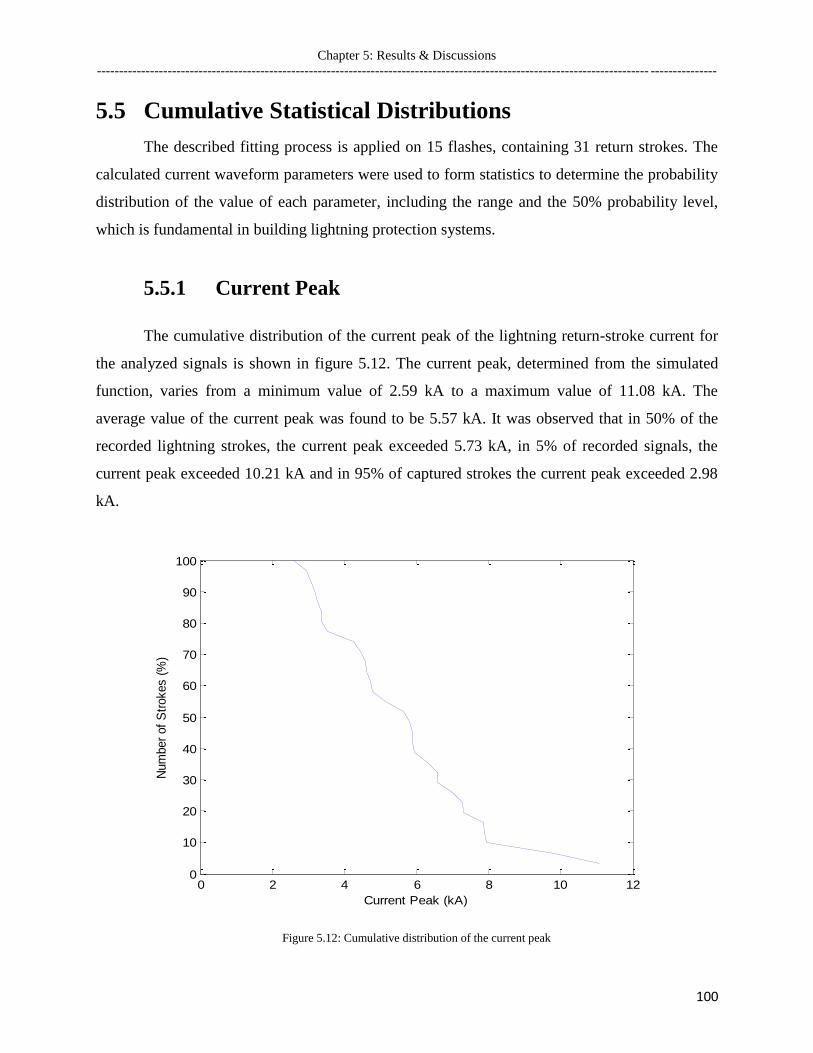
Chapter 5: Results & Discussions
----------------------------------------------------------------------------------------------------------------------------- ---------------
100
5.5 Cumulative Statistical Distributions
The described fitting process is applied on 15 flashes, containing 31 return strokes. The
calculated current waveform parameters were used to form statistics to determine the probability
distribution of the value of each parameter, including the range and the 50% probability level,
which is fundamental in building lightning protection systems.
5.5.1 Current Peak
The cumulative distribution of the current peak of the lightning return-stroke current for
the analyzed signals is shown in figure 5.12. The current peak, determined from the simulated
function, varies from a minimum value of 2.59 kA to a maximum value of 11.08 kA. The
average value of the current peak was found to be 5.57 kA. It was observed that in 50% of the
recorded lightning strokes, the current peak exceeded 5.73 kA, in 5% of recorded signals, the
current peak exceeded 10.21 kA and in 95% of captured strokes the current peak exceeded 2.98
kA.
Figure 5.12: Cumulative distribution of the current peak
0 2 4 6 8 10 120
10
20
30
40
50
60
70
80
90
100
Num
ber
of
Str
okes (
%)
Current Peak (kA)

Chapter 5: Results & Discussions
----------------------------------------------------------------------------------------------------------------------------- ---------------
101
5.5.2 Maximum Steepness
For the maximum steepness, its cumulative distribution is shown in Figure 5.13. The
lightning signals analyzed had a minimum value of 11.65 kA/µs and maximum value of 54.68
kA/µs for the maximum steepness. The average value for the maximum steepness was found to
be 31.33 kA/µs. In 95% of the signals, the maximum steepness came to be higher than 14.31
kA/µs and in 5% of the cases the maximum steepness was higher than 51.21 kA / µs. The 50%
probability value for the maximum steepness was found to be 34.31 kA/µs.
Figure 5.13: Cumulative distribution of the maximum steepness
0 10 20 30 40 50 600
10
20
30
40
50
60
70
80
90
100
Num
ber
of
Str
okes (
%)
Maximmum Steepness (kA/ s)

Chapter 5: Results & Discussions
----------------------------------------------------------------------------------------------------------------------------- ---------------
102
5.5.3 Risetime to the Current Peak
The 10% to 90% risetime to the current peak for each of the analyzed signals was
determined from the simulated function. Figure 5.14 shows the cumulative distribution of the
current risetime. The minimum recorded risetime to the current peak was 124 ns while the
maximum recorded value was 524 ns with an average of 242.3 ns. It is important realize this
large range of variation in the current risetime when designing lightning protection systems. For
the analyzed signals, the current risetime exceeds 143 ns, 211 ns and 481 ns in 95%, 50% and
5% of the cases, respectively.
.
Figure 5.14: Cumulative distribution of the risetime to the current peak
0 0.1 0.2 0.3 0.4 0.5 0.60
10
20
30
40
50
60
70
80
90
100
Num
ber
of
Str
okes (
%)
Risetime (s)

Chapter 5: Results & Discussions
----------------------------------------------------------------------------------------------------------------------------- ---------------
103
5.5.4 Decay Time from the Current Peak
The decay time of the current peak is an important waveform parameter. The 90% to 10%
current decay time from the current peak for each of the analyzed signals was determined. The
cumulative distribution of the current decay time is shown in Figure 5.15. The minimum value of
the current decay time was found to be 65.88 µs with maximum value of 537.13 µs. The average
value of the current decay time is 255.64 µs. In 95% of the cases, the current decay time exceeds
75.26 µs and in 5% of the cases, it exceeds 523.6 µs. The 50% probability value of the current
decay time is 261.3 µs.
Figure 5.15: Cumulative distribution of the decay time from the current peak
0 100 200 300 400 500 6000
10
20
30
40
50
60
70
80
90
100
Num
ber
of
Str
okes (
%)
Decay Time (s)

Chapter 5: Results & Discussions
----------------------------------------------------------------------------------------------------------------------------- ---------------
104
5.5.5 Current Pulse Width
The current pulse width at the half current peak level for each of the analyzed signals was
calculated by determining the time difference between the time at the 50% level of current peak
at the decay side of the current pulse and the 50% level of the current peak at the rising side of
the current pulse. Figure 5.16 shows the cumulative distribution of the current pulse width. The
minimum recorded current pulse width is 21.47 µs and the maximum recorded value is 157.51
µs, with an average of 83.99 µs. The large range of variation in current pulse width is important
to take into consideration by engineers working on lightning protection methods. For the
analyzed signals, the current pulse width 75.23 µs, 261.3 µs and 512.3 µs in 95%, 50% and 5%
of the cases, respectively.
Figure 5.16: Cumulative distribution of the current pulse width
0 20 40 60 80 100 120 140 1600
10
20
30
40
50
60
70
80
90
100
Num
ber
of
Str
okes (
%)
Current Pulse Width Half Peak (s)
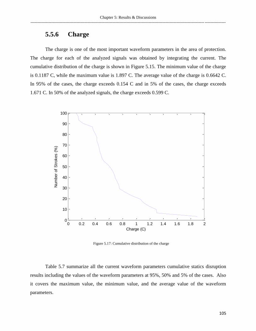
Chapter 5: Results & Discussions
----------------------------------------------------------------------------------------------------------------------------- ---------------
105
5.5.6 Charge
The charge is one of the most important waveform parameters in the area of protection.
The charge for each of the analyzed signals was obtained by integrating the current. The
cumulative distribution of the charge is shown in Figure 5.15. The minimum value of the charge
is 0.1187 C, while the maximum value is 1.897 C. The average value of the charge is 0.6642 C.
In 95% of the cases, the charge exceeds 0.154 C and in 5% of the cases, the charge exceeds
1.671 C. In 50% of the analyzed signals, the charge exceeds 0.599 C.
Figure 5.17: Cumulative distribution of the charge
Table 5.7 summarize all the current waveform parameters cumulative statics disruption
results including the values of the waveform parameters at 95%, 50% and 5% of the cases. Also
it covers the maximum value, the minimum value, and the average value of the waveform
parameters.
0 0.2 0.4 0.6 0.8 1 1.2 1.4 1.6 1.8 20
10
20
30
40
50
60
70
80
90
100
Num
ber
of
Str
okes (
%)
Charge (C)

Chapter 5: Results & Discussions
----------------------------------------------------------------------------------------------------------------------------- ---------------
106
Table 5.7: Summary of the current waveform parameters cumulative statistics distribution
Waveform Parameter Minimum Maximum Average 5% 50% 95%
Current Peak ( kA ) 2.895 11.08 5.572 10.21 5.73 2.98
Maximum Steepness
( kA/µs ) 11.65 54.68 31.3261 51.21 34.31 14.31
Risetime to Current Peak
( µs ) 0.124 0.524 0.2423 0.481 0.211 0.143
Decay Time from current
peak ( µs ) 65.88 537.13 255.64 523.6 261.3 75.26
Current Pulse Width
( µs ) 21.47 157.51 83.99 512.3 261.3 75.23
Charge ( C ) 0.1187 1.897 0.6642 1.671 0.5986 0.1542

Chapter 6: Conclusions and Recommendations
----------------------------------------------------------------------------------------------------------------------------- ---------------
107
Chapter 6
Conclusions and Recommendations
The main purpose for the study was to model the lightning return-stroke current,
measured at the CN Tower through which the current waveform parameters are calculated.
Although many simulating functions have been proposed, Heidler function and the Pulse
function were considered for the lightning return-stroke current modeling.
From the previous results it was concluded that the current derivative fitting yield better
results for simulating the measured signal than the current fitting. The initial values of the
analytical parameters of a given function were estimated. Using artificial digital signals, free of
noise and reflection, proved to be very efficient in the process of initial value estimations and the
evaluation simulation functions.
Previously, the fitting process involved the first impulse only of the measured current
derivative signal ignoring the decaying part to avoid reflections due to the tower‟s structure
discontinuities. The decoupling behavior of the Pulse and Heidler functions helped in dividing
the signal into three parts and in avoiding the use of the second part of the signal, which is highly
distorted by the reflection, in the fitting process. The third part was used for estimating the decay
time constant (τ2) and the other parameters were estimated from the first part of the signal
(mainly the rise portion of the signal). Results showed that τ2 and Imax have the same value for
both simulating functions (the Pulse and Heidler functions).
Finally, using a time forcing constraint for the maximum steepness of the current for
fitting the rising part of the signal with the estimated values of τ2 and Imax, the fitting process was
reduced to a single parameter estimation and the comparison between the Pulse and Heidler
functions was carried out. Although Heidler function is widely used in fitting the return-stroke
current signal, the Pulse function proved to be the better fit for the lightning return-stroke current
measured at the CN Tower.
The described fitting process represents the best method to reach the optimal value for
simulating the measured signal, not only by fitting the full measured signal including the decay
part but also by calculating all current waveform parameters. Using this fitting process for the
Pulse function all current waveform parameters were calculated. The calculated current

Chapter 6: Conclusions and Recommendations
----------------------------------------------------------------------------------------------------------------------------- ---------------
108
waveform parameters for 15 flashes, containing 31 return strokes, were used to form statistics to
determine the probability distribution of the value of each parameter, including the range and the
50% probability level, which is fundamental in building lightning protection systems.
The cumulative distribution can be improved by analyzing more lightning return-stroke
current signals. Using the lighting return-stroke currents collected from the tower since 1991, a
more extensive statistics can be achieved.
Also, the Pulse function can be improved for better fitting of the lighting return-stroke
current, which results in more accurate current waveform parameter values. This can be done by
introducing another term of forming a modified Pulse function, which will have eight analytical
parameters.
Although this work was preformed for modelling the CN Tower lightning return-stroke
current signals, it can be equally used for other lightning-related signals. Furthermore, this
research can be applied to a variety of signals, including those encountered in biomedical
applications, such as the heart-related electrical signals.

References
----------------------------------------------------------------------------------------------------------------------------- ---------------
109
REFERENCES
[1] F. Rachidi, W.Janischewskyj, A. M. Hussein, C. A. Nucci, S. Guerrieri, B. Kordi, and J. S.
Chang, “Current and Electromagnetic field associated with lightning return-stroke to tall
tower”, IEEE Transaction on Electromagnetic Compatibility, vol. 43, no. 3, pp. 356-367,
August 2001.
[2] V. A. Rakov and M. A. Uman, “Review and evaluation of lightning return stroke models
including some aspects of their application,” IEEE Transactions on Electromagnetic
Compatibility, vol. 40, no. 4, pp. 403-426, November 1998.
[3] Z. Feizhou and L. Shanghe, “A New Function to Represent the Lightning Return-Stroke
Current”, IEEE Transactions on Electromagnetic Compatibility, vol. 44, no. 4, pp. 595-
597, November 2002.
[4] M. Milewski and A. M. Hussein, “Evaluation of tall-structure lightning return-stroke model
using CN Tower data,” 19th
International Conference on Electromagnetic Disturbances,
pp. 180-185, Bialystok, Poland, Sept. 23-25, 2009.
[5] M. Milewski and A.M. Hussein, “Lightning Return-Stroke Transmission Line Model
Based on CN Tower Lightning Data and Derivative of Heidler Function”, IEEE Canadian
Conference on Electrical and Computer Engineering, pp. 1861-1866, Niagara Falls,
Ontario, May 4-7, 2008.
[6] K. Bitner and A.M. Hussein, “Modelling of the CN Tower lightning return-stroke current
derivative,” 28th
International Conference on Lightning Protection, pp. 261-266,
Kanazawa, Japan, September 2006.
[7] R.D. Jones, “On the use of tailored return-stroke current representation to simplify the
analysis of lightning effect on systems”, Transactions of the American Institute of
Electrical Engineers, Electromagnetic Compatibility, pp. 95-96, 1977.
[8] R.L. Gardner, Baker L., Baum C.E., Andersh D.J., “Comparison of lightning with public
domain HEMP waveforms on the surface of an aircraft”, 6th
EMC Symposium, pp.175-180,
Zurich, 1985.
[9] A.M. Hussein, W. Janischewskyj, M. Milewski, V. Shostak, W. Chisholm, J.S. Chang
”Current waveform parameters of CN Tower lightning return strokes,” Journal of
Electrostatics, vol. 60, pp.149-162, March 2004.

References
----------------------------------------------------------------------------------------------------------------------------- ---------------
110
[10] Vladimir A. Rakov, Martin A. Uman, Lightning Physics and Effects, Cambridge University
Press, Florida, 2003.
[11] Martin A. Uman, The Lightning Discharge, Academic Press Inc., Orlando, Florida, 1987.
[12] Earle R. Williams, “The Electrification of Thunderstorm,” Scientific America, no. 11, pp.
88-99, November 1988.
[13] Martin A. Uman, Understanding Lightning, Bek Technical Publications Inc., Carnegie,
Pennsylvania, 1971.
[14] R.B. Anderson, A.J. Eriksson, “Lightning Parameters for Engineering Applications,”
Electra, vol. 96, pp.65-105, 1980.
[15] W. Janischewskyj, A.M. Hussein, V. Shostak and P. Dzurevych, “Characterization of the
Current Wavefront Parameters of Lightning Strikes to the CN Tower in Toronto,” 8th
International Symposium on High Voltage Engineering, Yokohama, Japan, 1993.
[16] K.B. McEachron, “Lightning to the Empire State Building,” Journal of the Franklin
Institute, vol. 227, pp. 149-217, 1939.
[17] K.B. McEachron, “Lightning to the Empire State Building,” Transactions AIEE, vol. 60,
pp. 885-889, September 1941.
[18] A.M. Hussein, W. Janischewskyj, J.S. Chang, V. Shostak, W.A. Chisholm, P. Dzurevych
and Z.I. Kawasaki, “Simulation Measurment of Lightning Paramters for Strokes to the
Toronto Canadian National Tower,” Journal of Geophysical Reaserch, vol. 100, no. D5,
pp. 8853-8861, May 1995.
[19] W. Janischewskyj, A.M. Hussein, V. Shostak, I. Rusan, J.-X. Li and J.S. Chang, “Statistics
of Lightning Strikes to the Toronto National Canadian Tower (1978-1995),” IEEE
Transactions on Power Delivery, vol. 12, no. 3, pp. 1210-1221, July 1997.
[20] A.M. Hussein, W. Janischewskyj, M. Milewski, V. Shostak, J.S. Chang and W. Chishlom,
“Return-Stroke Current Waveform Parameters of Lightning to the CN Tower (1992-
2001),” International Conference of Lightning Protection, pp. 161-166, Cracow, Poland,
September 2003.
[21] V. Shostak, M. Wiacek and D. Tam, Report on the New Rogowski Coil Calibration, The
University of Toronto, Toronto, Canada, May 1998.

References
----------------------------------------------------------------------------------------------------------------------------- ---------------
111
[22] F. Heidler, J.M. Cavetic, B.V. Santic, “Calculation of Lightning current parameters”, IEEE
Transactions on Power Delivery. Vol. 14, No. 2, pp. 399-404, April 1999.
[23] F. Heidler, J.M. Cavetic, “A Class of Analytical Functions to Study the Lightning Effects
Associated with the Current Front”, European Transaction on Electrical Power. Vol. 12,
No. 2, pp. 141 – 150, April 2002.
[24] Chen Yazhou, Liu Shanghe, Wu Xiaorong, Zhang Feizhou, "A New Kind of Channel-base
Current Function," 3rd
International symposium on Electromagnetic Compatibility, pp.
304-307, May 2002.