comparison of conventional and advanced pavement design

Comparison of Conventional and

Advanced Pavement Design Methods with

Ontario Case Studies

by

Faraz Forghani

A thesis

presented to the University of Waterloo

in fulfillment of the

thesis requirement for the degree of

Master of Applied Science

in

Civil Engineering

Waterloo, Ontario, Canada, 2020

©Faraz Forghani 2020

ii

AUTHOR'S DECLARATION

This thesis consists of material all of which I authored or co-authored: see Statement of Contributions

included in the thesis. This is a true copy of the thesis, including any required final revisions, as accepted

by my examiners.

I understand that my thesis may be made electronically available to the public.

iii

Statement of Contributions

This thesis is partially the product of co-authored publications as follows, but modified slightly to

respect the flow of this thesis:

Chapter 5

▪ Forghani, F., Tighe, S., Henderson, V., Becke, M., Soares, R., & Haichert, R. (2020). Impact

of Road Geometry and Thickness on Pavement Behaviour using PSIPave 3D™.

Transportation Association of Canada.

iv

Abstract

Many methods have been used to effectively design a pavement structure that carries the required traffic

loads. In Canada, American Association of State Highway and Transportation Officials 93 (AASHTO

93), Shell Pavement Design (Shell), and Mechanistic-Empirical Pavement Design Guide (MEPDG) are

examples of pavement design methods. AASHTO 93 and Shell simplify the effects of loading by using

equivalent single axle loads which do not truly capture the effect of truck configurations. Other

parameters that AASHTO 93 and Shell do not address are environmental conditions, loading effects of

truck configurations, road geometry, or the behaviour of materials within the pavement structure.

MEPDG has begun to address some of these limitations, but the models have not been finalized and

require local calibrations for result accuracy.

University of Waterloo has partnered with PSI Technologies Inc. to evaluate the conventional design

strategies in Canada using a mechanistic pavement design method, PSIPave 3DTM. This method uses

three-dimensional modelling to evaluate the pavement responses under traffic loads considering the

effects of road geometry and truck configuration. PSIPave 3DTM outputs the normal and shear strains

anywhere in the pavement structure. Designs were provided for three road sections in Hamilton, Ontario

using AASHTO 93, Shell and MEPDG. The pavement structure for each road design were ran in

PSIPave 3DTM to evaluate different cases of geometry, tire types and bus configurations.

Based on these findings, the greatest impact of geometry was observed in the subgrade side slope but

was found to have minimal effects on the normal strains under the loading. In comparison to the

traditional dual tires (11R22.5), the super singles (455/55R22.5) were found to cause more damage

(fatigue and shear) in the upper layers and it was found that the effect of tire pressure dissipates as the

structure is investigated closer to the subgrade layer. The effect of changing bus configurations has an

effect on the strains as well. As the single axle is changed to a tandem axle, a major strain reduction

occurred. In terms of fatigue damage, an increase by a factor of approximately 2 was observed for the

number of load repetitions to fatigue failure whereas changing to dual tires on a single axle only causes

an increase by a factor of 1.34.

v

Acknowledgements

I would like to express my sincerest thanks to my supervisors Professor Susan Tighe and Professor

Vimy Henderson for their continuous support throughout my research and for their tremendous

knowledge, motivation, and patience. I am honored to have been under their supervision throughout

my time at the university. I would also like to thank the rest of the thesis committee: for their comments

and useful feedback towards improving my thesis.

I would like to acknowledge the staff at PSI Technologies Inc. for providing feedback and access to

PSIPave 3DTM, including Dan Pickel, Roberto Soares, Rielle Haichert, Curtis Berthelot, and Austin

Huang. I would also like to thank Mike Becke from the City of Hamilton for providing data for this

research.

I also want to thank my friends and classmates at Centre for Pavement and Transportation Technology

(CPATT) for their assistance and support. This would not have been possible without their help and

guidance.

Lastly, I would of course like to thank my parents for providing me with the support throughout my

studies and getting me to where I am today.

Thank You

vi

Table of Contents

AUTHOR'S DECLARATION .............................................................................................................. ii

Statement of Contributions ................................................................................................................... iii

Abstract ................................................................................................................................................. iv

Acknowledgements ................................................................................................................................. v

List of Figures ....................................................................................................................................... ix

List of Tables ........................................................................................................................................ xi

List of Abbreviations .......................................................................................................................... xiii

Chapter 1 INTRODUCTION .................................................................................................................. 1

1.1 Research Motivation .................................................................................................................... 2

1.2 Research Objectives ..................................................................................................................... 3

1.3 Outline of the Thesis .................................................................................................................... 4

Chapter 2 LITERATURE REVIEW ....................................................................................................... 5

2.1 Background .................................................................................................................................. 5

Design Methodologies .......................................................................................................... 6

Conventional Pavement Design Methods ............................................................................. 7

2.1.2.1 American Association of State Highway and Transportation Officials 93 (AASHTO

93) .............................................................................................................................................. 8

2.1.2.2 Shell Flexible Design Charts (Shell) ............................................................................ 11

2.1.2.3 Mechanistic-Empirical Pavement Design Guide (MEPDG) ........................................ 12

PSIPave 3DTM ..................................................................................................................... 16

Fatigue Damage .................................................................................................................. 17

2.2 Summary .................................................................................................................................... 17

Chapter 3 METHODOLOGY AND DATA ......................................................................................... 19

3.1 Methodology .............................................................................................................................. 19

3.2 Design Inputs ............................................................................................................................. 21

Borehole Data ..................................................................................................................... 21

Traffic ................................................................................................................................. 21

3.2.2.1 MEPDG ........................................................................................................................ 22

3.3 Road Information ....................................................................................................................... 22

North Service Road ............................................................................................................. 22

Cannon Street ...................................................................................................................... 24

vii

Stone Church Road .............................................................................................................. 25

3.4 Modulus Values .......................................................................................................................... 27

Chapter 4 DESIGN AND ANALYSIS ................................................................................................ 28

4.1 Conventional Designs ................................................................................................................. 28

AASHTO 93 ........................................................................................................................ 28

4.1.1.1 North Service Road (NSR) ........................................................................................... 28

4.1.1.2 Cannon Street (CS) ....................................................................................................... 31

4.1.1.3 Stone Church Road (SCR) ............................................................................................ 33

Shell ..................................................................................................................................... 34


4.1.2.2 Cannon Street (CS) ....................................................................................................... 36


MEPDG ............................................................................................................................... 37


4.1.3.2 Cannon Street (CS) ....................................................................................................... 39


4.2 PSIPave 3DTM Analysis .............................................................................................................. 41

North Service Road ............................................................................................................. 41

4.2.1.1 Geometry ...................................................................................................................... 41

4.2.1.2 Layers Thicknesses and Material Properties ................................................................ 42

4.2.1.3 Loading ......................................................................................................................... 43

Cannon Street ...................................................................................................................... 44

4.2.2.1 Geometry ...................................................................................................................... 44


4.2.2.3 Loading ......................................................................................................................... 45

Stone Church Road .............................................................................................................. 46

4.2.3.1 Geometry ...................................................................................................................... 47


4.2.3.3 Loading ......................................................................................................................... 48

Chapter 5 RESULTS AND DISCUSSIONS ........................................................................................ 51

5.1 Impact of Road Geometry .......................................................................................................... 51

PSIPave 3D™ Normal Strains ............................................................................................ 51

viii

PSIPave 3D™ Shear Strains ............................................................................................... 53

5.1.2.1 Shear Strains in the Side Slope .................................................................................... 56

5.2 Impact of Tire Type ................................................................................................................... 60

PSIPave 3D™ Normal Strains ............................................................................................ 61

PSIPave 3D™ Shear Strains ............................................................................................... 64

5.3 Impact of Configuration ............................................................................................................. 65

PSIPave 3DTM Normal Strains ............................................................................................ 66

5.3.1.1 Fatigue Comparison ..................................................................................................... 69

PSIPave 3DTM Shear Strains ............................................................................................... 71

Chapter 6 CONCLUSION .................................................................................................................... 74

References ............................................................................................................................................. 76

Appendix A AASHTO 93 Designs ....................................................................................................... 80

Appendix B PSIPave Geometry Charts ................................................................................................ 81

ix

List of Figures

Figure 1-1: Severe Pavement Distress .................................................................................................... 1

Figure 1-2: Flow Chart of Research Objectives ..................................................................................... 3

Figure 2-1: Flexible Pavement Structure ................................................................................................ 5

Figure 2-2: AASHTO 93 Nomograph .................................................................................................... 9

Figure 2-3: MEPDG Pavement Rehabilitation Selection Process (Ministry of Transportation Ontario,

2019) ..................................................................................................................................................... 15

Figure 3-1: PSIPave Survey Van .......................................................................................................... 19

Figure 3-2: North Service Road (Google, 2020) .................................................................................. 23

Figure 3-3: NSR Frost Susceptibility Criteria Chart ............................................................................ 24

Figure 3-4: Cannon Street .................................................................................................................... 24

Figure 3-5: CS Frost Susceptibility ...................................................................................................... 25

Figure 3-6: Stone Church Road ............................................................................................................ 26

Figure 3-7. SCR Frost Susceptibility .................................................................................................... 26

Figure 4-1 PSIPave 3DTM North Service Road Geometry ................................................................... 42

Figure 4-2 NSR PSIPave 3DTM B-Train Loading Input ....................................................................... 43

Figure 4-3: Tire Types (OTRUSA, 2020) ............................................................................................ 44

Figure 4-4: NSR PSIPave 3DTM Tractor-Trailer Loading Input ........................................................... 46

Figure 4-5: Bus Configurations in Ontario (Government of Ontario, 2019) ........................................ 47

Figure 4-6: SCR PSIPave 3DTM Bus 1 Configuration .......................................................................... 49

Figure 4-7: SCR PSIPave 3DTM Bus 2 Configuration ........................................................................ 49

Figure 4-8: SCR PSIPave 3DTM Bus 3 Configuration ........................................................................ 49

Figure 5-1: NSR Peak Tensile Strain in Asphalt Binder (μm/m) ......................................................... 52

Figure 5-2: NSR Peak Compressive Strain in Subgrade (μm/m) ......................................................... 53

Figure 5-3: NSR Peak Shear Strain in Asphalt Top Course (μm/m) .................................................... 54

Figure 5-4: NSR Peak Shear Strain in Granular Subbase (μm/m) ....................................................... 54

Figure 5-5: NSR Peak Shear Strain in Silty Clay Subgrade (μm/m) .................................................... 55

Figure 5-6: NSR Shear Strain Contour for AASHTO 93 Thicknesses, 3.95 m Shoulder, 6.4:1 Side

Slope ..................................................................................................................................................... 56

Figure 5-7: NSR Shear Strain Contour for MEPDG Thicknesses, 0.7 m Shoulder, 1.7:1 Side Slope . 57

Figure 5-8: NSR Peak Shear Strain in Subgrade Side Slope (μm/m) ................................................... 58

Figure 5-9: NSR Shear Strain for AASHTO 93 Thicknesses, 0.7 m Shoulder, 1.7:1 Side Slope ........ 59

x

Figure 5-10: NSR Shear Strain for AASHTO 93 Thicknesses, 3.95 m Shoulder, 6.4:1 Side Slope ... 60

Figure 5-11: CS Peak Tensile Strain in Asphalt Binder Course (μm/m) ............................................. 61

Figure 5-12: CS Peak Compressive Strain in Subgrade (μm/m) ......................................................... 62

Figure 5-13: CS Vertical Displacement in Subgrade (11R22.5) .......................................................... 63

Figure 5-14: CS Peak Shear Strain in Asphalt Top Course (μm/m) .................................................... 64

Figure 5-15: CS Peak Shear Strain in Subbase (μm/m) ....................................................................... 64

Figure 5-16: CS Peak Shear Strain in Subgrade (μm/m) ..................................................................... 65

Figure 5-17: SCR Peak Tensile Strain in Asphalt Binder Course (μm/m) .......................................... 66

Figure 5-18: SCR Peak Compressive Strain in Subgrade (μm/m) ....................................................... 67

Figure 5-19: SCR Tensile Strain in Asphalt Binder Course (Bus 1) ................................................... 68



Figure 5-22: SCR Peak Shear Strain in Asphalt Top Course (μm/m) ................................................. 71

Figure 5-23: SCR Peak Shear Strain in Base (μm/m) .......................................................................... 72

Figure 5-24: SCR Peak Shear Strain in Subbase (μm/m) .................................................................... 72

Figure 5-25: SCR Peak Shear Strain in Subgrade (μm/m) .................................................................. 73

xi

List of Tables

Table 2-1: City of Hamilton Recommended Minimum Pavement Thicknesses .................................... 6

Table 2-2: Flexible Pavement Design Methods in Canada (Tighe, Pavement Asset Design and

Management Guide, 2013) ..................................................................................................................... 7

Table 2-3: Inputs for AASHTO 93 Method ........................................................................................... 8

Table 2-4: Inputs for Shell .................................................................................................................... 11

Table 2-5: Inputs for MEPDG .............................................................................................................. 13

Table 2-6: Inputs for PSIPave 3DTM ..................................................................................................... 16

Table 2-7: Benefits and Challenges of Each Pavement Design Method .............................................. 18

Table 4-1: Traffic Data for North Service Road ................................................................................... 29

Table 4-2: AASHTO 93 Inputs for North Service Road (Hajek et al., 2008) ...................................... 30

Table 4-3: Design for North Service Road (AASHTO 93) .................................................................. 31

Table 4-4: Traffic Data for Cannon Street............................................................................................ 32

Table 4-5: AASHTO 93 Inputs for Cannon Street ............................................................................... 32

Table 4-6: Design for Cannon Street (AASHTO 93) ........................................................................... 33

Table 4-7: Traffic Data for Stone Church Road ................................................................................... 33

Table 4-8. AASHTO 93 Inputs for Stone Church Road ....................................................................... 34

Table 4-9: Design for Stone Church Road (AASHTO 93)................................................................... 34

Table 4-10: Finding the MAAT for Shell Design (Government of Canada, 2019) ............................. 35

Table 4-11: Design for North Service Road (Shell) ............................................................................. 36

Table 4-12: Design for Cannon Street (Shell) ...................................................................................... 37

Table 4-13: Design for Stone Church Road (Shell) ............................................................................. 37

Table 4-14. NSR AASHTOWare Outputs for MEPDG ....................................................................... 38

Table 4-15: CS AASHTOWare Outputs for MEPDG .......................................................................... 39

Table 4-16: SCR AASHTOWare Outputs for MEPDG ....................................................................... 40

Table 4-17: Final Designs for NSR ...................................................................................................... 42

Table 4-18: Load per Axle for North Service Road ............................................................................. 44

Table 4-19: Final Designs for CS ......................................................................................................... 45

Table 4-20: Load per Axle for Cannon Street ...................................................................................... 46

Table 4-21: Final Designs for SCR ...................................................................................................... 48

Table 4-22: Load per Axle for Stone Church Road .............................................................................. 50

Table 5-1: North Service Road Thickness and Load Summary ........................................................... 51

xii

Table 5-2: Cannon Street Thickness and Load Summary .................................................................... 61

Table 5-3: Stone Church Road Thickness and Load Summary ........................................................... 66

Table 5-4: Allowable Number of Fatigue Repetitions ......................................................................... 70

Table 5-5: Predicted Number of Load Repetitions .............................................................................. 70

xiii

List of Abbreviations

AADT Average Annual Daily Traffic

AADTT Average Annual Daily Truck Traffic

AASHO American Association of State Highway Officials

AASHTO American Association of State Highway Transportation Officials

CGRA Canada Good Roads Association

CL Silty Clay

CPATT Centre for Pavement and Transportation Technology

CS Cannon Street

DDHV Directional Design Hour Volume

DF Directional Factor

EB Eastbound

ESAL Equivalent Single Axle Load

FEM Finite Element Modelling

FHWA Federal Highway Administration

FWD Falling Weight Deflectometer

GPR Ground Penetrating Radar

HMA Hot Mix Asphalt

IRI International Roughness Index

LIDAR Light Detection and Ranging

LTPP Long-Term Pavement Performance

MAAT Mean Annual Air Temperature

ME Mechanistic Empirical

MEPDG Mechanistic-Empirical Pavement Design Guide

MMAT Mean Monthly Air Temperature

MTO Ministry of Transportation Ontario

NCHRP National Cooperative Highway Research Program

NSR North Service Road

ON Ontario

OPAC Ontario Pavement Analysis of Costs

PCC Portland Cement Concrete

PG Performance Grade

PSI Pavement Serviceability Index

SCR Stone Church Road

SN Structural Number

SP Superpave

TAC Transportation Association of Canada

USCS United Soil Classification System

WB Westbound

1

Chapter 1

INTRODUCTION

A pavement structure allows the safe and smooth transportation of people and goods which stimulates

economic growth. Each road should provide a smooth, durable, and skid-resistant surface. A typical

flexible pavement structure consists of Hot Mix Asphalt (HMA), granular base, and granular subbase.

The primary goal in pavement design is to design a structure that can distribute the stresses from traffic

to the underlying layers without damaging the subgrade. Pavements will start to deteriorate at a faster

rate if proper design, construction, and maintenance procedures are not followed.

Pavement distresses, such as rutting and cracking, not only lead to a decrease in the lifetime of the

pavement but can also cause user discomfort and dangerous accidents. An example of a severe

pavement distress is shown in Figure 1-1. This figure highlights the importance of considering the

effects of climate and drainage in the pavement structure. The surface of this road could be slightly

sloped towards the ditches to help mitigate the moisture damage to the HMA layer. Moreover, these

geometry parameters also have an impact on the strains and having a better understanding of the

pavement behaviour can be beneficial in coming up with a design that is more representative of the

road’s conditions.

Figure 1-1: Severe Pavement Distress

2

Through the introduction of better design strategies, the need for maintenance can be minimized which

saves on direct and user costs (traffic delays). A better design strategy will also maximize the

investment by the owner.

1.1 Research Motivation

With pavement design continuously undergoing development, it is beneficial to highlight and compare

the features of each method. The purpose of this comparison is so that the designers are aware of the

implications of using each method. Empirical methods such as American Association of State Highway

and Transportation Officials 93 (AASHTO 93), the most common design method used in Canada

(Tighe, Pavement Asset Design and Management Guide, 2013), does not consider the effects of climate

nor truly account for material behaviour under loads. These methods convert all types of load into an

equivalent single axle load which does not properly represent the impact of different truck

configurations.

Shell Pavement Design Method (Shell) considers the Mean Annual Air Temperature (MAAT) in its

analysis and introduces a mechanistic aspect that uses layer elastic theory to calculate the strains and

stresses based on the given inputs. The designer refers to a set of charts to obtain the pavement layer

thicknesses. In addition to climate, Mechanistic-Empirical Pavement Design Guide (MEPDG) also

includes axle load spectra in its analysis. However, MEPDG is still undergoing development and does

not consider the impact of road geometry and shear stresses on the pavement performance.

Additionally, accurate results require the local calibration of the global pavement distress models which

can be a costly and time-consuming task. Not all of the current tools consider many of the important

factors that have an impact on pavement performance such as climate, geometry, shear stresses and the

configuration of trucks. Therefore, the limitations of conventional design methods are becoming

apparent.

Currently, there are a few pavement design methods available to designers to help determine the

required thicknesses for a pavement structure. Pavement design strategies can be further developed to

address these inputs in the design process. The main motivation of this research is to compare and

accomplish designs with each pavement design method to show the benefits and limitations of each

tool.

3

1.2 Research Objectives

The objectives of this research are the following:

1) Describe and highlight the features of three common pavement design methods including the

benefits and limitations of each.

a. Design a reconstruction pavement structure using each of the discussed pavement design

methods for three selected roads in Hamilton, ON. The roads are North Service Road,

Cannon Street, and Stone Church Road.

2) Using PSIPave 3DTM, evaluate the impact of geometry, bus configurations and tire types on

pavement performance. The nine pavement structures developed in objective 1 will be used in

PSIPave 3DTM.

3) Analyze the outputs from PSIPave 3DTM and using the normal and shear strains, compare each

pavement structure obtained from conventional design methods.

Figure 1-2 presents an overall schematic of the objectives. As a summary, the objectives are to show

the contributions and limitations of current pavement design tools, and how considerations on road

geometry and shear strains can further enhance pavement design strategies using Ontario case

studies.

Figure 1-2: Flow Chart of Research Objectives

Identify the benefits and limitations of conventional pavement design methods

Pavement structure design for North Service Road, Canon Street and Stone Church Road

Receive a thickness from AASHTO 93, Shell and MEPDG

Analyze each pavement structure using PSIPave 3DTM

4

1.3 Outline of the Thesis

Chapter 1 Introduction: This chapter provides a short background about the topic, the research

motivation, the research objectives, and the outline for the rest of this thesis.

Chapter 2 Literature Review: This chapter provides background information about design

methodologies, conventional pavement design methods (in detail including their model, inputs,

drawbacks), PSIPave 3DTM, and fatigue damage analysis.

Chapter 3 Methodology and Data: This chapter provides information on the methodology of the

study and relevant information about the three road sections considered in this work.

Chapter 4 Design and Analysis: This chapter shows the design process for AASHTO 93, MEPDG,

and Shell. These designs are then analyzed in PSIPave 3DTM to evaluate the effect of road geometry,

wide-base tires versus conventional dual-tires, and bus configurations.

Chapter 5 Results and Discussions: This chapter discusses the results obtained from PSIPave 3DTM

considering the peak normal and shear strains in PSIPave 3DTM.

Chapter 6 Conclusions: This chapter presents the key conclusions derived from the results.

5

Chapter 2

LITERATURE REVIEW

2.1 Background

The function of a pavement structure is to distribute the stresses from the load effectively throughout

the layers. 64.1% of the pavements in Canada are flexible and 0.3% are rigid according to a survey by

Transportation Association of Canada (TAC) in 2010 (Tighe, Pavement Asset Design and Management

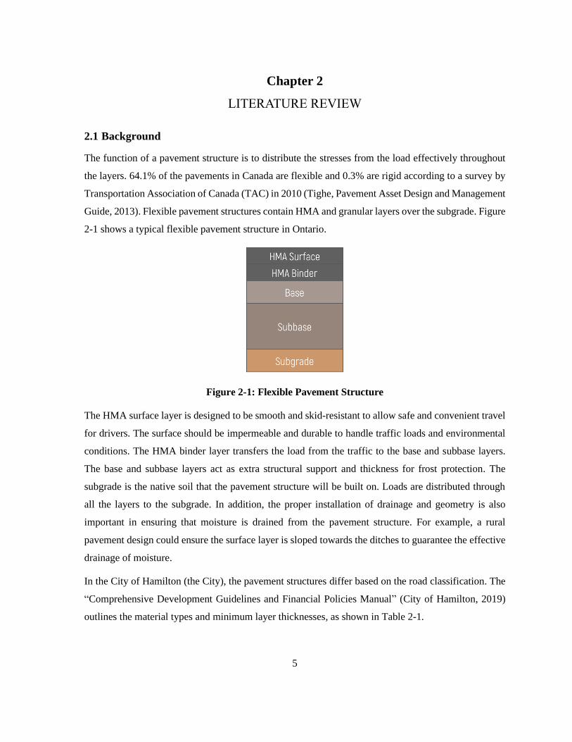
Guide, 2013). Flexible pavement structures contain HMA and granular layers over the subgrade. Figure

2-1 shows a typical flexible pavement structure in Ontario.

Figure 2-1: Flexible Pavement Structure

The HMA surface layer is designed to be smooth and skid-resistant to allow safe and convenient travel

for drivers. The surface should be impermeable and durable to handle traffic loads and environmental

conditions. The HMA binder layer transfers the load from the traffic to the base and subbase layers.

The base and subbase layers act as extra structural support and thickness for frost protection. The

subgrade is the native soil that the pavement structure will be built on. Loads are distributed through

all the layers to the subgrade. In addition, the proper installation of drainage and geometry is also

important in ensuring that moisture is drained from the pavement structure. For example, a rural

pavement design could ensure the surface layer is sloped towards the ditches to guarantee the effective

drainage of moisture.

In the City of Hamilton (the City), the pavement structures differ based on the road classification. The

“Comprehensive Development Guidelines and Financial Policies Manual” (City of Hamilton, 2019)

outlines the material types and minimum layer thicknesses, as shown in Table 2-1.

6

Table 2-1: City of Hamilton Recommended Minimum Pavement Thicknesses

City of

Hamilton

Top Course

Asphalt Binder Course

Granular

A

Granular

B II

Roads (Rural and Urban)

Collector 40 mm Superpave

9.5 PG 58-28

100 mm Superpave

19 PG 58-28 150 mm 300 mm

Arterial

50 mm Superpave

12.5 FC1 or FC2

PG 58H or V-28

110 mm Superpave

19 PG 58-28H or V-

28

150 mm 450 mm

The mixes used by the City are Superior Performing Asphalt Pavements (Superpave) mixes which bring

a new performance-based asphalt binder specification. The performance grade (PG) is selected based

on the climate of the design location. To select the performance grade, 7-day maximum pavement

temperature and minimum pavement temperature of the region are determined. The maximum and

minimum pavement temperatures are selected to be resistant against rutting and cracking, respectively

(The Federal Highway Administration, 1995). A PG58-28 binder is designed considering a 7-day

maximum pavement temperature of 58°C and a minimum pavement temperature of -28°C. Granular

materials, which are commonly used for the base and subbase, are a mix of aggregates. The design

thickness of the HMA mixes and granular materials shown in Table 2-1 can also be obtained by using

conventional pavement design methods.

Design Methodologies

Pavement structures have been designed with the following methodologies, but each come with their

limitations:

▪ Experience-based methodology is based on previous experience in the region. Given the

pavement type, the designer refers to a set of tables and deduces the pavement thicknesses.

The designer should refer to experience tables specific to a given region as thicknesses can

vary depending on different traffic loads and climates. Table 2-1 is an example of

experience-based methodology.

▪ Empirical methodology is developed based on experiments and experience. For example, the

AASHTO 93 empirical model is based on a road test further explained in Section 2.1.2.1.

7

This model simplifies the design process by minimizing laboratory and field testing for each

specific design.

▪ Mechanistic-empirical methodology calculates the stresses, strains, and deflection and

relates these responses to the pavement performance. This methodology typically requires

more inputs, but they result in better predicted outputs. The most common mechanistic-

empirical method is MEPDG which is used to predict the pavement distresses. This

pavement design method is explained in Section 2.1.2.3.

The methods commonly used across Canada are shown in Table 2-2 based on the Table outlined in the

2013 Pavement Asset Design Management Guide by Transportation Association of Canada.

Table 2-2: Flexible Pavement Design Methods in Canada (Tighe, Pavement Asset Design and

Management Guide, 2013)

Agency General Design Methods

Alberta AASHTO 93

British Columbia AASHTO 93

Saskatchewan Shell Method

Asphalt Institute

Manitoba AASHTO 93/MEPDG (new construction)

Canada Good Roads Association (CGRA)/MEPDG (rehabilitation)

Ontario

AASHTO 93

Ontario Pavement Analysis of Costs (OPAC)

Routine (Empirical) Method

Quebec AASHTO 93

Chausée 2

New Brunswick AASHTO 93

Rebound Values

Prince Edward Island Asphalt Institute

Nova Scotia AASHTO 93

Correlation Charts using AADT and grain size of subgrade

Newfoundland and Labrador Standard Section Used

Yukon State of Alaska Design Method

Public Works and Government

Services Canada (Federal)

AASHTO 93

State of Alaska Design Method

Conventional Pavement Design Methods

The pavement design methods considered in this research are: AASHTO 93, Shell, and MEPDG. The

following section will discuss the basis, limitations, inputs, and outputs of the conventional pavement

8

design methods compared in this thesis. It will also discuss the capability of each method to accomplish

rehabilitation designs.

2.1.2.1 American Association of State Highway and Transportation Officials 93 (AASHTO 93)

AASHTO 93 is an empirical pavement design method developed by the American Association of

State Highway and Transportation Officials in 1961, but the explanation and design procedure will be

based on the 1993 revision used in Ontario (American Association of State Highway and

Transportation Officials, 1993). This method is based on a 27 million-dollar test in Ottawa, IL for

both flexible and rigid pavement structures (Pavement Interactive, n.d.). Performance measurements

such as roughness, distress, strains, and pavement serviceability index (PSI) were collected during

this test phase.

Based on these measurements, a series of empirical equations and nomographs were developed. The

AASHTO 93 equation outputs the structural number of the pavement structure which represents the

structural strength of the given pavement structure based on the given road conditions (American

Association of State Highway and Transportation Officials, 1993). The inputs for a flexible pavement

design (asphalt) are shown in Table 2-3.

Table 2-3: Inputs for AASHTO 93 Method

Inputs Description

Reliability Probability of intended performance

S0 Standard error of traffic and performance prediction

W18 Number of 80 kN single-axle loads

∆ PSI The change between initial and terminal serviceability index

Mr Resilient modulus of the subgrade

A guide is available in Ontario to help designers determine what inputs to use as typical values for an

AASHTO 93 design (Hajek et al., 2008). Once all the inputs are obtained, the required structural

number is calculated with Equation 2-1.

log10(W18) = 𝑍𝑅𝑆0 + 9.36 log10(𝑆𝑁 + 1) − 0.20 +log10 (

∆PSI4.2 − 1.5

)

0.40 +1094

(𝑆𝑁 + 1)5.19

+ 2.32 log10(𝑀𝑅) − 8.07

Equation 2-1

9

where

W18 = Number of 80KN single axle loads

ZR = Standard normal variate

S0 = Standard error of traffic and performance prediction

SN = Structural number

∆PSI = The difference between initial and terminal serviceability

MR = Resilient modulus of the subgrade

Alternatively, the nomograph, shown in Figure 2-2, could be used to obtain the required structural

number. This figure shows a typical design process for the given values.

Figure 2-2: AASHTO 93 Nomograph

Once the required structural number is determined, the designer needs to select the thicknesses for

each layer. To find the structural number of the design, Equation 2-2 can be used (American

Association of State Highway and Transportation Officials, 1993).

𝑆𝑁∗ = ∑ 𝑎1𝐷1 + 𝑎𝑖𝐷𝑖𝑚𝑖

𝑛

𝑖=2

Equation 2-2

where

n = number of layers

ai = Material coefficient of layer i

Di = Thickness of layer i

10

mi = Drainage coefficient of layer i

The inputs and coefficients for Ontario could be found in the “Adaptation and Verification of

AASHTO Pavement Design Guide for Ontario Conditions” (Hajek et al., 2008). The structural

number of the selected layer composition must be greater than the required structural number in order

to satisfy the design requirement.

Other than designing new and reconstructed pavement structures, the AASHTO 1993 method also

provides a guideline for overlay design. The overlay structural number is determined by taking the

difference between the expected structural number (considering future traffic) and the effective

structural number of current structures shown in Equation 2-3. The coefficients for selected

rehabilitation methods such as pulverizing are shown in the AASHTO design document for Ontario

(Hajek et al., 2008).

𝑆𝑁𝑂𝐿 = 𝑆𝑁𝑓 − 𝑆𝑁𝑒𝑓𝑓

Equation 2-3 (Hajek et al., 2008)

where

SNOL = The structural number of the required overlay

SNf = The expected structural number considering future traffic

SNeff = The effective structural number (measured from falling weight deflectometer testing)

The challenges associated with AASHTO 93 are the following:

▪ This method is solely based on observations and measurements made during a two-year test

with only a specific climate in mind. The only climate consideration in AASHTO 93 is the time

it takes for the moisture to be drained through a drainage coefficient. The Long-Term Pavement

Performance (LTPP) program has indicated that under normal traffic, 36% of the pavement

deteriorations are caused by climate and subgrade (The Federal Highway Administration,

2016). Therefore, proper consideration of climate in the design process will be beneficial in the

long-term performance of the pavement structure.

▪ For the traffic input, mixed traffic is converted to 80 kN equivalent single axle loads (ESAL)

which has been shown to simplify the effects of traffic on the pavement performance (Dinegdae

& Birgisson, 2016).

▪ It does not truly account for material behaviour under loading.

11

▪ Material properties are indicated through a layer coefficient. No matter what type of HMA is

used, the layer coefficient for it is 0.44 and therefore AASHTO 93 cannot distinguish between

quality differences of the same material.

▪ Engineering judgement is required as AASHTO 93 does not consider extra thickness for frost

protection.

AASHTO 93 simplifies the design process with a global equation. Many regions and agencies continue

using the method because the inputs are easy to gather and do not require much laboratory or field

testing.

2.1.2.2 Shell Flexible Design Charts (Shell)

Shell is a mechanistic-empirical model developed by Shell International Petroleum Co. in 1963 and

further updated in 1978. This method treats the pavement structure as a three-layer system which

designs based on the maximum horizontal tensile strain at the bottom of the asphalt layer and the

maximum vertical compressive strain at the top of the subgrade (Shell International Petroleum

Company Limited, 1978). The purpose of the horizontal tensile strain is to control bottom-up cracking

(fatigue cracking) and vertical compressive strain is to control subgrade deformation (rutting). These

failure methods are briefly discussed in Section 2.1.2.3. Table 2-4 shows the inputs for Shell’s flexible

design method.

Table 2-4: Inputs for Shell

Inputs Description

ESAL Traffic volume (80 kN equivalent single axle load)

Dynamic Modulus Subgrade and unbound materials moduli

MAAT Mean annual air temperature

Mix Code Fatigue/stiffness characteristics of asphalt

Shell also adopts the standard 80 kN equivalent single axle load for its traffic parameter. The dynamic

modulus values could be assigned from Chart E of the manual based on the material type if laboratory

testing is not feasible or available. The MAAT can be calculated by referring to the climatic information

from a given weather station in the region. The mix code contains three parts that determine the

properties of the HMA.

12

▪ S and F variables determine the fatigue and stiffness characteristics (1 used for typical mixes

and 2 used for mixes that have high void percentages or are open-graded).

▪ The last part of the mix code determines the penetration resistance of the HMA, which is

now replaced by a performance grade system. Two penetration values can be chosen: 50 or

100.

Based on these inputs, the designer refers to a chart that corresponds to these inputs and determines the

design thicknesses of the structural layers. The total unbound layer thickness can be initially chosen by

the designer and Shell provides the breakdown of the base and subbase layers based on their

corresponding modulus.

The Shell method does provide steps for overlay design as well. The process involves using the MAAT

and using deflection measurements to estimate the asphalt effective thickness, subgrade modulus, and

original design life. Future design life and the overlay thickness are determined whether the original

failure criterion was based on subgrade strain or asphalt fatigue.

The challenges associated with Shell are the following:

▪ Only allows for flexible pavement designs.

▪ Also uses ESAL which has been shown to simplify the effects of traffic on the pavement

performance (Dinegdae & Birgisson, 2016).

▪ Limited set of design charts available therefore interpolation is required if a value is in-

between.

▪ Engineering judgement is required as Shell does not consider extra thickness for frost

protection.

2.1.2.3 Mechanistic-Empirical Pavement Design Guide (MEPDG)

MEPDG is a mechanistic-empirical model, which was developed under the National Cooperative

Highway Research Program (NCHRP) (Li et al., 2011). This method was first completed in 2004 but

is still undergoing further updates and development. The mechanistic aspect of this method calculates

the stresses, strains, and deflections, and the empirical aspect relates these responses to predict the

pavement distresses throughout its lifetime. MEPDG uses Jacob Uzan Layered Elastic Analysis

(JULEA) and 2D-FEM to output the stresses and strains (Li et al, 2011). This method does not output

layer thicknesses, but instead requires thicknesses to do its analysis. A design with this method involves

13

changing the pavement thickness until a satisfactory result is achieved in all failure criteria. As this is

an iterative design process, the designer finds the optimal design for a given project based on the

performance threshold determined by the region. This method allows for three hierarchical levels

available for design (ARA, Inc., ERES Consultants Division, 2004):

▪ Level 1: Site specific data – laboratory and field testing are required to find the properties for

materials, traffic distribution, climate in the chosen site.

▪ Level 2: Agency database or values estimated through correlations

▪ Level 3: Typical values used in the region

Table 2-5 shows the inputs for MEPDG.

Table 2-5: Inputs for MEPDG

Inputs Description

Environment Temperature and moisture

Materials Properties and thicknesses of each material used

Traffic Loads, classifications, configuration and forecasting

Reliability Probability that design will be under distress limits

Aguib has identified environment and traffic as two primary inputs in pavement performance (Aguib,

2013). Additionally, it was found that temperature was the most impactful factor in climate. In Virginia,

it was found that a 5% increase in temperature has a potential to reduce the pavement service life by

20% (Qiao et al., 2013). At hot temperatures, the asphalt layers become soft which can lead to surface

rutting whereas at cold temperatures, the asphalt layers can experience low-temperature cracking.

Consequently, moisture advects through the surface cracks and causes debonding of the asphalt

membranes with the aggregates which further damages the pavement (Yang & Ning, 2011). MEPDG

can predict the accumulation of damage to predict pavement performance over time. One of the goals

for pavement design is to minimize the distresses. TAC predicts that MEPDG will be the most used

pavement design method after calibration and validation (Tighe, 2013). A study in Manitoba that used

default and local load spectra values, concluded that default MEPDG values are not representative of

local conditions (Ahammed et al., 2011).

The design process is carried out through the software “AASHTOWare Pavement ME Design” which

enhances the use of MEPDG. The outputs are pavement distresses such as terminal international

roughness index (IRI), permanent deformation of total pavement, bottom-up fatigue cracking, top-

14

down fatigue cracking, and thermal cracking. Based on the road classification, the predicted distresses

outputted by MEPDG would have to be below a given set of thresholds set by the region. The design

is considered satisfactory if it is below the threshold for all predicted distresses. These distresses are

briefly discussed below and predicted based on empirical transfer functions (Huang, 2004):

▪ IRI measures the longitudinal surface profile (roughness) in the wheel path.

▪ Bottom-up fatigue cracking is caused as a result of the maximum tensile strain at the bottom of

the HMA layer and propagates towards the surface.

▪ Top-down cracking is caused as a result of the critical shear strain in thick pavements and

cracks initiate on the surface layer of the pavement structure. However, the top-down

cracking failure mechanism is still not fully understood and therefore it is not used as an

acceptance criterion.

▪ Permanent deformation (total pavement) is caused as a result of HMA and subgrade rutting.

HMA rutting could occur due to a weak mix, subgrade rutting is caused as a result of the

maximum compressive strain on the subgrade due to traffic loading. The subgrade deflects

and the pavement structure follows the same path downwards, causing ruts in the wheel path

which leads to major rideability issues.

▪ Thermal cracking is a challenge in areas that experience cold climates and has two types: low-

temperature cracking and thermal fatigue cracking. Low-temperature cracks are formed as a

result of shrinkage due to the hardening of the binder. Thermal fatigue cracks are caused by the

tensile strains in the pavement due to the variation in temperature.

Tighe et al. (2008) has found that distresses such as rutting and alligator cracking will worsen in the

future, but low-temperature cracking will be less prominent.

This method can also be used for rehabilitation purposes. The condition of the pavement must be

assessed at the time of rehabilitation. Existing material moduli can be backcalculated from the

deflection basins obtained from Falling Weight Deflectometer (FWD) testing. Cores could also help

provide insight into the material type and thicknesses. These inputs are entered into MEPDG with local

calibration factors and ran with the expected traffic and climate of the given test section to see if the

performance criteria pass in all the distress types. If any of the distresses fall below the performance

threshold set by the region, the design must provide a thicker overlay to pass the design and reran to

15

check for passing (Module 8: Asphalt Overlays of Asphalt Pavements). The pavement rehabilitation

selection process is shown in Figure 2-3.

Figure 2-3: MEPDG Pavement Rehabilitation Selection Process (Ministry of Transportation

Ontario, 2019)

The challenges associated with MEPDG are the following:

▪ This method relies on significant input from the user, which may require further

laboratory/field testing based on the level of hierarchy chosen.

▪ The license of AASHTOWare is expensive to purchase.

▪ Since the transfer functions are empirical, local calibration of the models are required to output

more accurate results. Local calibration is the process of changing the coefficients for the global

16

models to reduce the standard error between predicted and observed local distresses (Tarefder

& Rodriguez-Ruiz, 2013). This is a time-consuming and costly task.

▪ As the method is undergoing development, some of the global models are still not fully

calibrated and finalized.

PSIPave 3DTM

Finite element modelling (FEM) has been used before in pavement design, but most designers refer to

general-use FEM software such as ABAQUS. Liu et al. (2017) found that ABAQUS takes too much

time for pavement structural analysis purposes. PSI Technologies Inc., an engineering firm based in

Saskatchewan, Canada that specializes in transportation infrastructure and mine water management,

has developed a three-dimensional modelling tool used to analyze pavement structures and determine

the displacements, stresses, and strains at any location. This tool considers the impact of road geometry

on normal stresses and shear stresses which are only attainable through a three-dimensional analysis.

Shear forces are generated from braking, accelerating and standard motion of the wheel that occurs

while driving (Global Road Technology, 2016). Literature has found that shear stresses are one of the

major causes of deteriorations, such as rutting and top-down cracking, observed in the pavement (Su et

al., 2008). These peak shear stresses occur at the edge of the tires and are more critical in thick HMA

pavements while longitudinal strains are the critical strains in thin HMA pavements (Al-Qadi & Wang,

2009). This is likely due to the thick HMA layers effectively reducing the longitudinal tensile strains.

Considering these factors, pavement designs can be analyzed in PSIPave 3DTM for a better

understanding of the pavement behavior. Table 2-6 shows the inputs for PSIPave 3DTM.

Table 2-6: Inputs for PSIPave 3DTM

Inputs Description

Material Properties Layer thicknesses, modulus of each layer, and Poisson's ratio

Truck Configuration Maximum load per axle, interaxle spacing, group spread, track width,

tire type and pressure

Road Geometry Road width, shoulder width, side slope, surface slope, ditch depth

Designs could use typical modulus values for the region. The cross section of the pavement depends

on whether it is an urban or rural pavement design. The pavement structure will include shoulders for

rural designs and include curbs for urban designs. The loading is based on any truck of the designer’s

choosing, with fully customizable axle/tire configurations. In addition to the truck configuration, the

17

type of tire used is also an important consideration in evaluating the pavement responses in PSIPave

3DTM. The truck loading is transferred through the tire to the pavement layers therefore tire-pavement

interaction is valuable in calculating the pavement responses. Once all the inputs are obtained and

entered, PSIPave 3DTM generates a mesh on the given pavement structure and performs a finite element

analysis to determine the stresses, strains, and displacements anywhere along the structure. These

results can then be used by a designer for further analysis, such as fatigue damage analysis.

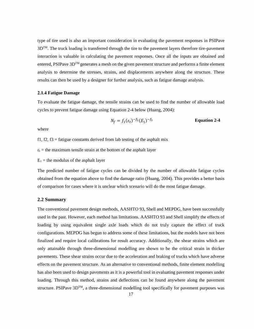
Fatigue Damage

To evaluate the fatigue damage, the tensile strains can be used to find the number of allowable load

cycles to prevent fatigue damage using Equation 2-4 below (Huang, 2004):

𝑁𝑓 = 𝑓1(𝜀𝑡)−𝑓2(𝐸1)−𝑓3 Equation 2-4

where

f1, f2, f3 = fatigue constants derived from lab testing of the asphalt mix

εt = the maximum tensile strain at the bottom of the asphalt layer

E1 = the modulus of the asphalt layer

The predicted number of fatigue cycles can be divided by the number of allowable fatigue cycles

obtained from the equation above to find the damage ratio (Huang, 2004). This provides a better basis

of comparison for cases where it is unclear which scenario will do the most fatigue damage.

2.2 Summary

The conventional pavement design methods, AASHTO 93, Shell and MEPDG, have been successfully

used in the past. However, each method has limitations. AASHTO 93 and Shell simplify the effects of

loading by using equivalent single axle loads which do not truly capture the effect of truck

configurations. MEPDG has begun to address some of these limitations, but the models have not been

finalized and require local calibrations for result accuracy. Additionally, the shear strains which are

only attainable through three-dimensional modelling are shown to be the critical strain in thicker

pavements. These shear strains occur due to the acceleration and braking of trucks which have adverse

effects on the pavement structure. As an alternative to conventional methods, finite element modelling

has also been used to design pavements as it is a powerful tool in evaluating pavement responses under

loading. Through this method, strains and deflections can be found anywhere along the pavement

structure. PSIPave 3DTM, a three-dimensional modelling tool specifically for pavement purposes was

18

developed by PSI Technologies Inc. This research investigates how to address limitations of current

methods and whether considering parameters that accurately represent the road conditions such as road

geometry, truck configurations, and tire types will have a major effect on the pavement performance.

The benefits and drawbacks of each pavement design method are shown in Table 2-7. Some engineering

judgement is required when designing with all of these tools such as ensuring the pavement structure

is sufficient to protect against frost damage.

Table 2-7: Benefits and Challenges of Each Pavement Design Method

Pavement Design

Methods Benefits Drawbacks

AASHTO 93

- There is an alternative to solving

the complex empirical equation

with a chart - When there is uncertainty or not a

lot of inputs available to the

designer, this method is a good

option for design.

- Free

- Its empirical nature does not

accurately replicate the pavement

conditions.

- Does not truly account for material

behavior under loading

- Does not consider climate other than

the climate of the test location and

through drainage properties.

- Uses ESAL which simplifies the

impact of traffic on pavement

performance

Shell - Does not require many inputs

- Simplified the design process

with a set of charts

- Only allows for flexible pavement

designs

- Requires interpolation as there is

only a set of limited charts available

- Uses ESAL which simplifies the

impact of traffic on pavement

performance

MEPDG

-Gives the damage accumulation

over time using performance

prediction models if pavement

thicknesses and other inputs are

known.

- Requires a lot of inputs for the

highest-level accuracy, lab and field

testing are required which means

longer and more expensive designs.

- It must be locally calibrated for

accurate results.

- Still undergoing development

- Expensive design software

19

Chapter 3

METHODOLOGY AND DATA

3.1 Methodology

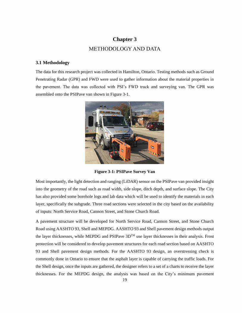
The data for this research project was collected in Hamilton, Ontario. Testing methods such as Ground

Penetrating Radar (GPR) and FWD were used to gather information about the material properties in

the pavement. The data was collected with PSI’s FWD truck and surveying van. The GPR was

assembled onto the PSIPave van shown in Figure 3-1.

Figure 3-1: PSIPave Survey Van

Most importantly, the light detection and ranging (LiDAR) sensor on the PSIPave van provided insight

into the geometry of the road such as road width, side slope, ditch depth, and surface slope. The City

has also provided some borehole logs and lab data which will be used to identify the materials in each

layer, specifically the subgrade. Three road sections were selected in the city based on the availability

of inputs: North Service Road, Cannon Street, and Stone Church Road.

A pavement structure will be developed for North Service Road, Cannon Street, and Stone Church

Road using AASHTO 93, Shell and MEPDG. AASHTO 93 and Shell pavement design methods output

the layer thicknesses, while MEPDG and PSIPave 3DTM use layer thicknesses in their analysis. Frost

protection will be considered to develop pavement structures for each road section based on AASHTO

93 and Shell pavement design methods. For the AASHTO 93 design, an overstressing check is

commonly done in Ontario to ensure that the asphalt layer is capable of carrying the traffic loads. For

the Shell design, once the inputs are gathered, the designer refers to a set of a charts to receive the layer

thicknesses. For the MEPDG design, the analysis was based on the City’s minimum pavement

20

thicknesses outlined in Table 2-1. If these thicknesses provide satisfactory results, it will be selected as

the MEPDG design. Otherwise, the thicknesses will be increased until the predicted distresses are below

the thresholds set by region. These thickness designs are then be compared using PSIPave 3DTM. The

designer can get a better understanding of the pavement behaviour by using three-dimensional

modelling which provides information about the strains, stresses and displacements anywhere in the

structure. Each road section is used to evaluate a different scenario:

▪ North Service Road will be used to evaluate a total of twelve cases to assess the impact of

geometry (three different design thicknesses with four different geometric cases).

o Geometry Case 1: Narrow shoulder, steep slope

o Geometry Case 2: Narrow shoulder, gradual slope

o Geometry Case 3: Wide shoulder, steep slope

o Geometry Case 4: Wide shoulder, gradual slope

▪ Cannon Street will be used to evaluate a total of six cases to assess the impact of wide-base

tires versus conventional dual tires (three different design thicknesses with two different tires).

o Tire Type 1: Conventional dual tires (11R22.5)

o Tire Type 2: New generation wide-base tires (455/55R22.5)

▪ Stone Church Road will be used to evaluate a total of nine cases to assess the impact of different

bus loading and axle configurations.

o Bus 1: Single axles, single tires

o Bus 2: Tandem drive axle, single tires

o Bus 3: Articulated bus with dual tires

The cases will be explained more in detail in Section 4.2. Results of each case will be discussed

thoroughly.

21

3.2 Design Inputs

Borehole Data

The borehole and coring data for each road were provided by the City. Using this data, the material and

thickness of each layer can be identified. For the purpose of this study, the borehole and coring data is

useful in determining the subgrade material. Designers must ensure there is sufficient HMA and

granular thickness to protect the underlying subgrade. The frost susceptibility of the subgrade must also

be evaluated using the frost susceptibility criteria chart (Transportation Association of Canada, 1997).

The evaluation of this is due to frost heave taking place in cold conditions. In freezing conditions, the

moisture in the soils turn to ice and cause an expansion in the soil. If the material type is highly

susceptible to frost, thicker pavement structures must be considered for extra protection against frost

action. Granular layers provide an insulation blanket to help restrict the movement of water within the

depth of the pavement structure (Arjun). Coarse-grained gravels are used as they are less susceptible to

frost action. As a rule of thumb, pavement designers aim for a total pavement structure thickness that

meets 50% of the frost depth (Pavement Interactive, n.d.). In the City of Hamilton, the frost depth is

1.2 m (Terraprobe, 2013), and therefore the minimum frost depth pavement designers provide to protect

against frost action is 600 mm. For the selected road sections explained further in the paper, all subgrade

materials were silty clay.

Traffic

The traffic data was also provided by the city. This data included traffic counts on an interval of 15

minutes. The peak count of buses and trucks was the most valuable information in the traffic data as

motorcycles (FHWA category 1), passenger cars (FHWA category 2), and four-tire single units (FHWA

category 3) are neglected in the calculation of ESALs. The pavement damage caused by these vehicles

is negligible compared to the damage caused by trucks and buses (Heavy Lifting-Estimating Roadway

Loading, 2018). There is a rule of thumb that peak traffic accounts for 8-12% of Average Annual Daily

Traffic (AADT). Equation 3-1 is used to solve for the AADT using the directional design hour volume

(DDHV) (U.S. Department of Transportation, 2018).

𝐴𝐴𝐷𝑇 =

𝐷𝐷𝐻𝑉

𝐾 𝑥 𝐷

Equation 3-1

22

where

DDHV = Directional design hour volume

K = Proportion of AADT occurring in the peak hour

D = Proportion of traffic driving in the major direction

A conservative design approach was taken when calculating the AADT from morning and afternoon

peak values, of which the higher AADT value was retained. The D factor was not used in this

calculation as the AADT in only one direction was required. For the traffic distribution, all buses were

treated as two or three axle buses, Federal Highway Administration (FHWA) vehicle class 4. The site-

specific truck distribution was unknown, therefore typical values in the region were utilized (Swan et

al., 2008).

3.2.2.1 MEPDG

The traffic inputs mentioned in this section were consistent throughout the three different road sections.

The values used in the design were specifically for conditions observed in Ontario and are gathered

from the “Ontario’s Default Parameters for AASHTOWare Pavement ME Design Interim Report –

2019” (Ministry of Transportation Ontario, 2019). Monthly adjustments and hourly distributions of

traffic were not considered as recommended by the interim report. The Average Annual Daily Truck

Traffic (AADTT) were calculated from the traffic data presented by the City.

3.3 Road Information

Based on the availability of data and the inputs required for the conventional pavement design methods

and PSIPave 3DTM, the following three road sections were chosen for this analysis:

1. North Service Road (Truck Route)

2. Cannon Street (Truck Route and Bus Route)

3. Stone Church Road (Truck Route and Bus Route)

North Service Road

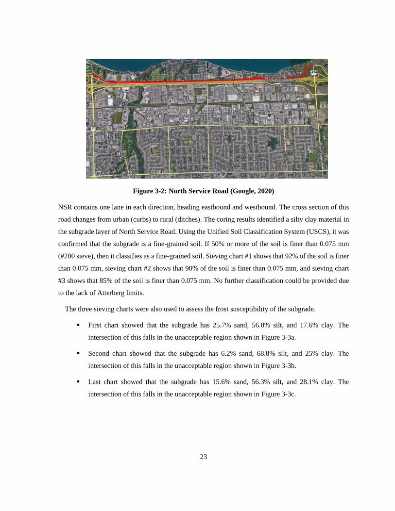
North Service Road (NSR) is a two-lane road in Hamilton, Ontario shown in Figure 3-2. This section

is approximately 5.36 centerline kilometers in length from Centennial Parkway to Fruitland Road. The

road is classified as an urban collector. Coring data was available for the entirety of this section. This

includes data about the material used in each layer, the thickness of the material, and the core location.

23

Figure 3-2: North Service Road (Google, 2020)

NSR contains one lane in each direction, heading eastbound and westbound. The cross section of this

road changes from urban (curbs) to rural (ditches). The coring results identified a silty clay material in

the subgrade layer of North Service Road. Using the Unified Soil Classification System (USCS), it was

confirmed that the subgrade is a fine-grained soil. If 50% or more of the soil is finer than 0.075 mm

(#200 sieve), then it classifies as a fine-grained soil. Sieving chart #1 shows that 92% of the soil is finer

than 0.075 mm, sieving chart #2 shows that 90% of the soil is finer than 0.075 mm, and sieving chart

#3 shows that 85% of the soil is finer than 0.075 mm. No further classification could be provided due

to the lack of Atterberg limits.

The three sieving charts were also used to assess the frost susceptibility of the subgrade.

▪ First chart showed that the subgrade has 25.7% sand, 56.8% silt, and 17.6% clay. The

intersection of this falls in the unacceptable region shown in Figure 3-3a.

▪ Second chart showed that the subgrade has 6.2% sand, 68.8% silt, and 25% clay. The

intersection of this falls in the unacceptable region shown in Figure 3-3b.

▪ Last chart showed that the subgrade has 15.6% sand, 56.3% silt, and 28.1% clay. The

intersection of this falls in the unacceptable region shown in Figure 3-3c.

24

a) Sieve Chart 1 b) Sieve Chart 2 c) Sieve Chart 3

Figure 3-3: NSR Frost Susceptibility Criteria Chart

Cannon Street

Cannon Street (CS) is a three-lane street in Hamilton, Ontario shown in Figure 3-4. This section is

approximately 5.13 centerline kilometers in length from York Boulevard to Ottawa Street. The street

is classified as an urban collector which turns into a minor arterial between Sherman Ave. and York

Blvd. From Sherman Ave., the street becomes one-directional heading westbound towards York Blvd.

However, borehole data was only available for the east section of CS where the street is classified as

an urban collector.

Figure 3-4: Cannon Street

25

The east section of CS contains one lane in each direction, heading eastbound and westbound, with a

two-way turning lane in the middle. Cannon Street’s cross-section is urban (curbs) throughout the

whole street. The borehole data for this section also revealed a silty clay for the subgrade material. The

only sieve chart provided for this section showed that 87% of the material is finer than 0.075 mm (#200

sieve) which confirms a fine-grained soil according to the USCS. No further classification could be

provided due to the lack of Atterberg limits.

The sieving chart was also used to evaluate the frost susceptibility of the subgrade. The subgrade

material has 13.2% sand, 62.2% silt, and 24.6% clay. The intersection of these falls in the unacceptable

region shown in Figure 3-5.

Figure 3-5: CS Frost Susceptibility

Stone Church Road

Stone Church Road (SCR) is a three-lane road in Hamilton, Ontario shown in Figure 3-6. This section

is approximately 9.66 centerline kilometers in length from Mohawk Road to Dartnall Road shown

below. The road is classified as a minor arterial throughout the whole section. Borehole data was

available for the western half of this section.

26

Figure 3-6: Stone Church Road

SCR contains one lane in each direction, heading eastbound and westbound, with a two-way turning

lane in the middle. SCR’s cross-section is urban (curbs) throughout. The borehole data identified a silty

clay in the subgrade layer. Similarly, the sieving chart provided was used to verify a fine-grained soil

in the subgrade with 82.5% of the material being finer than 0.075 mm (#200 sieve). No further

classification could be provided due to the lack of Atterberg limits. To evaluate the susceptibility, it

was concluded that the subgrade material consisted of 19.8% sand, 64% silt, and 16.2% clay. This falls

inside the unacceptable region shown in Figure 3-7.

Figure 3-7. SCR Frost Susceptibility

27

The native subgrade material in all three road sections is highly susceptible to frost and a thicker

pavement structure is required to protect against frost damage.

3.4 Modulus Values

PSIPave 3DTM requires modulus values for the materials, so this section investigates which moduli

values are going to be used in this research. A collector road in the City uses a PG 58-28 binder and an

arterial road in the City uses a PG58-28H binder. The grade H binder is relatively new, and the mix is

intended to carry loads from a higher traffic. The PG58-28H mix has been shown to be equivalent to a

PG64-28 or a PG64-28P (Minnesota Department of Transportation, 2019). The modulus values used

were based at the 21.1°C and 10 Hz level which simulates normal traffic conditions (Baghaee

Moghaddam & Baaj, 2020). The asphalt modulus values used in each road section were based on the

availability of level 1 data and a performance that either met or went above the City’s minimum mix

requirements. For the granular and subgrade layers, average Ministry of Transportation Ontario (MTO)

values for Ontario’s conditions were used. North Service Road used a value of 25 MPa for the subgrade

value which is close to material being in its fair condition to be consistent with the value used in the

Shell design. For Cannon Street and Stone Church Road, the good condition material properties were

used as the modulus backcalculated from FWD testing showed a higher modulus.

28

Chapter 4

DESIGN AND ANALYSIS

4.1 Conventional Designs

The designs for AASHTO 93, Shell, MEPDG, and PSIPave are explained in this section.

AASHTO 93

4.1.1.1 North Service Road (NSR)

“The Adaptation and Verification of AASHTO Pavement Design Guide for Ontario Conditions”

provides the user with typical inputs necessary for an AASHTO 93 design in Ontario. The traffic data

provided by the City for North Service Road was used to determine the equivalent single axle loads

(ESALs). Equation 4-1 was used to calculate the ESALs for each road (Huang, 2004):

𝑊18 = 𝐴𝐴𝐷𝑇 𝑥 𝑇 𝑥 𝑇𝑓 𝑥 𝐿𝐷 𝑥 𝐷𝐹 𝑥 𝐺 𝑥 365 Equation 4-1

where

W18 = ESALs

AADT = Average annual daily traffic

T = Heavy vehicle percentage

TF = Truck factor (ESALs per truck)

LD = Lane distribution (how many trucks travel in the design lane)

DF = Directional factor (the percentage of AADT travelling in the specific direction)

G = Growth factor (the overall traffic growth throughout the pavement design life) G is calculated

with Equation 4-2 (Huang, 2004).

365 accounts for the number of days in a year.

𝐺 =

(1 + 𝑔)𝑛 − 1

𝑔 Equation 4-2

where

g = cumulative growth rate

n = years of design

29

AADT was calculated using Equation 3-1 and shown in Table 4-1. The following list explains how

the ESAL inputs were obtained.

▪ The following traffic distribution and the associated FHWA category used to calculate the

ESAL is shown below.

o Buses (16.1%), two axle six tire single unit (30%), three axle single unit (10%), four

or more axle single unit (2.5%), four or less axle single trailer (1.7%), five axle tractor

semitrailer (25.1%), six or more axle single trailer (12.6%), five or less axle multi

trailer (0%), six axle multi-trailer (0%), seven or more axle multi-trailer (1.7%)

▪ The heavy vehicle percentage was calculated using bus and truck traffic count, which were

used to denote heavy vehicle count, as a proportion of total traffic count.

▪ Typical truck factors were used for each FHWA category (Hajek et al., 2008).

▪ A lane distribution of 1 is used as there is only one lane in each direction.

▪ The directional factor is not applicable since the AADT is already calculated for the major

direction of traffic flow.

▪ A standard growth rate of 2% is used with a 20-year design life in Ontario since there was no

historical AADT available for NSR (Holt et al., 2011). For NSR, the growth factor, G, is 24.3.

Table 4-1: Traffic Data for North Service Road

Road Intersection Direction

Vehicle

Count

(AM)

Vehicle

Count

(PM)

AADT

(AM)

AADT

(PM)

ESAL

(106)

NSR

Millen (Jun

13)

WB 583 172 5830 1720 2.4

EB 107 389 1070 3890 0.7

Green (Jun

13)

WB 764 325 7640 3250 4.5

EB 48 393 480 3930 0.6

Drakes (Jun

13)

WB 866 328 8660 3280 4

EB 43 417 430 4170 0.6

ESALs were calculated using Equation 4-1, of which the highest value of 4.5 million (rounded up) was

retained. The silty clay subgrade was assigned a typical resilient modulus of 25 MPa, which identifies

the material in its fair condition. A flexible design for NSR (urban collector) would use the following

inputs summarized in Table 4-2.

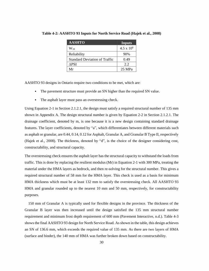
30

Table 4-2: AASHTO 93 Inputs for North Service Road (Hajek et al., 2008)

AASHTO Inputs

W18 4.5 x 106

Reliability 90%

Standard Deviation of Traffic 0.49

ΔPSI 2.2

Mr 25 MPa

AASHTO 93 designs in Ontario require two conditions to be met, which are:

▪ The pavement structure must provide an SN higher than the required SN value.

▪ The asphalt layer must pass an overstressing check.

Using Equation 2-1 in Section 2.1.2.1, the design must satisfy a required structural number of 135 mm

shown in Appendix A. The design structural number is given by Equation 2-2 in Section 2.1.2.1. The

drainage coefficient, denoted by m, is one because it is a new design containing standard drainage

features. The layer coefficients, denoted by “a”, which differentiates between different materials such

as asphalt or granular, are 0.44, 0.14, 0.12 for Asphalt, Granular A, and Granular B Type II, respectively

(Hajek et al., 2008). The thickness, denoted by “d”, is the choice of the designer considering cost,

constructability, and structural capacity.

The overstressing check ensures the asphalt layer has the structural capacity to withstand the loads from

traffic. This is done by replacing the resilient modulus (Mr) in Equation 2-1 with 300 MPa, treating the

material under the HMA layers as bedrock, and then re-solving for the structural number. This gives a

required structural number of 58 mm for the HMA layer. This check is used as a basis for minimum

HMA thickness which must be at least 132 mm to satisfy the overstressing check. All AASHTO 93

HMA and granular rounded up to the nearest 10 mm and 50 mm, respectively, for constructability

purposes.

150 mm of Granular A is typically used for flexible designs in the province. The thickness of the

Granular B layer was then increased until the design satisfied the 135 mm structural number

requirement and minimum frost depth requirement of 600 mm (Pavement Interactive, n.d.). Table 4-3

shows the final AASHTO 93 design for North Service Road. As shown in the table, this design achieves

an SN of 136.6 mm, which exceeds the required value of 135 mm. As there are two layers of HMA

(surface and binder), the 140 mm of HMA was further broken down based on constructability.

31

Table 4-3: Design for North Service Road (AASHTO 93)

Flexible Design Thickness

(mm)

Layer

Coefficient

Drainage

Coefficient SN

Design

SN

SP12.5 PG70-28P 60 0.44 1 26.4

136.6 SP19 PG64-28P 80 0.44 1 35.2

Granular A 150 0.14 1 21

Granular B Type II 450 0.12 1 54

4.1.1.2 Cannon Street (CS)

The borehole data towards the east of CS silty clay identified a silty clay material for the subgrade. This

is the section where CS is an urban collector, so most inputs remain the same other than traffic (W18).

Historical AADT was available for this road from 2013 to 2019 and was used to determine the growth

rate, g or the annual average change rate (AACR). AACR was calculated with Equation 4-3. The growth

rate was determined to be 1.05% for CS.

𝐴𝐴𝐷𝑇𝑓 = 𝐴𝐴𝐷𝑇𝑐 × (1 + 𝐴𝐴𝐶𝑅)𝑛 Equation 4-3

where

AADTf = Future AADT (veh/yr)

AADTc = Current AADT (veh/yr)

AACR = Annual average change rate

n = Number of forecasted years

The following traffic distribution and the associated FHWA category used to calculate the ESAL is

shown below:

▪ Buses (36.4%), two axle six tire single unit (22.9%), three axle single unit (7.6%), four or more

axle single unit (1.9%), four or less axle single trailer (1.3%), five axle tractor semitrailer

(19.1%), six or more axle single trailer (9.6%), five or less axle multi trailer (0%), six axle

multi-trailer (0%), seven or more axle multi-trailer (1.3%)

32

With a growth rate of 1.05% and the traffic distribution shown above, the following ESALs were

calculated and shown in Table 4-4.

Table 4-4: Traffic Data for Cannon Street

Intersection Direction

Vehicle

Count

(AM)

Vehicle

Count

(PM)

AADT

(AM)

AADT

(PM)

ESAL

(106)

Balmoral (Oct

01 2018)

WB 241 244 2410 2440 3.1

EB 168 199 1680 1990 1.8

Melrose (Oct

16 2019)

WB 461 368 4610 3680 1.9

EB 276 264 2760 2640 2.3

Lottridge (Oct

17 2019)

WB 365 328 3650 3280 2.3

EB 189 261 1890 2610 1.8

Hence, the ESAL used in this design is 3.1 million ESALs. Since the corrected backcalculated

modulus showed a higher value than the MTO fair condition, the good condition was used for both

Cannon Street and Stone Church Road. The resilient modulus value used for the silty clay is 35 MPa

which identifies the subgrade in its good condition (Hajek et al., 2008). A flexible design for CS

(urban collector) would use the following inputs summarized in Table 4-5.

Table 4-5: AASHTO 93 Inputs for Cannon Street

AASHTO Inputs

W18 3.1 x 106

Reliability 90%

Standard Error of Traffic 0.49

ΔPSI 2.2

Mr 35 MPa


for the pavement structure and 57.2 mm for the HMA layer to pass the overstressing check. Rounded

to the nearest 10 mm, the HMA should be a minimum of 130 mm. The Granular A thickness was

consistent at 150 mm throughout all the designs. The Granular B thickness was then increased to 400

mm to provide the structural capacity and extra frost protection. Table 4-6 shows the final AASHTO

93 design for CS. As shown in the table, this design achieves an SN of 126.2 mm, which exceeds the

required value of 116 mm. As there are two layers of HMA (surface and binder), the 130 mm of HMA

33

was further broken down based on constructability. The Granular B was increased by an extra 50 mm

to provide extra protection against frost as the subgrade was highly susceptible to frost.

Table 4-6: Design for Cannon Street (AASHTO 93)


(mm)

Layer

Coefficient

Drainage

Coefficient SN

Design

SN

SP12.5 PG58-28 50 0.44 1 26.4

126.2 SP19 PG64-28 80 0.44 1 30.8

Granular A 150 0.14 1 21

Granular B, Type II 400 0.12 1 48

4.1.1.3 Stone Church Road (SCR)

In Ontario, collectors and minor arterials share the same inputs in AASHTO 93 therefore traffic (W18)

remains to be the only difference in the inputs. The available historical data from 2014 to 2019 was

used to calculate a growth rate of approximately 2.8% using Equation 4-3.

▪ Buses (52.9%), two axle six tire single unit (17%), three axle single unit (5.7%), four or more

axle single unit (1.4%), four or less axle single trailer (0.9%), five axle tractor semitrailer

(14.1%), six or more axle single trailer (7.1%), five or less axle multi trailer (0%), six axle

multi-trailer (0%), seven or more axle multi-trailer (0.9%)

With a growth rate of 2.75% and the traffic distribution shown above, the following ESALs were

calculated and shown in Table 4-7.

Table 4-7: Traffic Data for Stone Church Road

Intersection Direction Vehicle

Count (AM)

Vehicle

Count (PM)

AADT

(AM)

AADT

(PM)

ESAL

(106)

Upper Gage (Nov 05,

19)

WB 564 740 5640 7400 4.6

EB 626 866 6260 8660 3.5

Upper Sherman (Nov

25, 19)

WB 638 731 6380 7310 5.6

EB 472 609 4720 6090 5.3

Upper Wentworth (Oct

29, 19)

WB 366 424 3660 4240 5.9

EB 348 487 3480 4870 5.5

Upper Wellington (Nov

25, 19)

WB 518 589 5180 5890 2.8

EB 402 715 4020 7150 3.2

Harrogate (Nov 26, 19) NB 886 497 8860 4970 2.7

SB 276 876 2760 8760 1.8

Golf Links (Nov 26, 19) NB 787 483 7870 4830 2.3

34

A flexible design for SCR (minor arterial) would use the following inputs summarized in Table 4-8.

Table 4-8. AASHTO 93 Inputs for Stone Church Road

AASHTO 93 Inputs

W18 5.9 x 106

Reliability 90%

Standard Error of Traffic 0.49

ΔPSI 2.2

Mr 35 MPa


for the pavement structure and 61 mm for the HMA layer to pass the overstressing check. Rounded to

the nearest 10 mm, the HMA thickness should be a minimum of 140 mm. Table 4-9 shows the final

AASHTO 93 design for SCR. As shown in the table, this design achieves an SN of 130.6 mm, which

exceeds the required value of 126 mm. As there are two layers of HMA (surface and binder), the 140

mm of HMA was further broken down based on constructability.

Table 4-9: Design for Stone Church Road (AASHTO 93)


(mm)

Layer

Coefficient

Drainage

Coefficient SN

Design

SN

SP12.5 FC1 PG64-28 60 0.44 1 26.4

130.6 SP19 PG64-28 80 0.44 1 35.2

Granular A 150 0.14 1 21

Granular B, Type II 400 0.12 1 48

Shell


The design procedure explained below follow the standards outlined in the “Shell Pavement Design

Manual” (Shell International Petroleum Company Limited, 1978). Once the inputs (traffic, mix code,

mean annual air temperature (MAAT), layer moduli) are determined, the designer can refer to a set of

curves to determine the thicknesses of their pavement.

Shell adopts the standard 80 KN standard axle load, same as the one used in AASHTO 93 (4.5 million

ESALs), as its traffic parameter. The new flexible pavement designs for all three road sections will use

a typical mix (not open-graded). Higher penetration values are better suited for colder climates and as

35

a result, 100 was chosen for the City (Pavement Interactive, n.d.). S1-F1-100 is the final mix code for

each design. The modulus of unbound materials was assigned using Chart E from the manual. The

moduli chosen for the subgrade (Silty Clay), base layer (Granular A) and subbase layer (Granular B),

were 25 MPa, 800 MPa and 400 MPa, respectively (Shell International Petroleum Company Limited,

1978). Shell requires a minimum modulus for unbound base layers to produce thicker designs as a

protection against frost damage and the moduli that were chosen kept this in consideration.

The effect of climate is included in the Shell method in terms of the mean annual air temperature

(MAAT). To calculate the mean annual air temperature, the mean monthly air temperatures (MMAT)

of climate station “Hamilton A”, short for Hamilton airport, were used (Government of Canada, 2019).

This weather station is located approximately 19 km away from North Service Road, 12 km away from

Cannon Street, and 5.6 km away from Stone Church Road.

Chart W included in the Shell design manual assigned a weight to each temperature to consider the

daily and monthly variation (Shell International Petroleum Company Limited, 1978). Table 4-10 shows

the mean monthly air temperature and the associated weights for each month.

Table 4-10: Finding the MAAT for Shell Design (Government of Canada, 2019)

Month MMAT (°C) W-MAAT (°C)

Jan -6.9 0.027

Feb -4.4 0.037

March -1.3 0.055

April 5.5 0.14

May 11.5 0.346

June 17.7 0.78

July 22.1 1.55

Aug 20 1.04

Sept 17 0.71

Nov 10 0.28

Oct 0.4 0.071

Dec -1.2 0.055

The average of the W-MAATs is then converted back to a temperature using Chart W. Based on Shell,

the mean annual air temperature for Hamilton, Ontario, was found to be 13.2°C. The temperature was

rounded to 12°C based on the available Shell curves.

36

The Shell design for North Service Road has the following inputs:

▪ Traffic: 4.5x106

▪ Layer Moduli (MPa): 25 (Silty Clay), 800 (Granular A), 400 (Granular B)

▪ Mix Code: S1-F1-100

▪ MAAT (°C): 12

The initial unbound layer thickness was chosen to be 600 mm to provide sufficient frost protection.

Using Chart HN 13, Shell recommends 135 mm of HMA, 240 mm of Granular A and 360 mm of

Granular B for the unbound layers. The final Shell design for North Service Road is shown in Table

4-11. Based on constructability, the HMA layer is further broken down into the two layers (surface and

binder). The thicknesses were obtained from the chart and were therefore left at their corresponding

values.

Table 4-11: Design for North Service Road (Shell)


(mm)

SP12.5 PG70-28P 60

SP19 PG64-28P 75

Granular A 260

Granular B, Type II 340


For Cannon Street, the only difference in inputs for the Shell design is in the traffic (ESALs). Since the

selected subgrade modulus for Cannon Street is 35 MPa and there are two available subgrade values

for the shell curves (25 MPa and 50 MPa). A subgrade modulus of 25 MPa was chosen for a

conservative design. Additionally, extra cases of Shell thicknesses will be analyzed in PSIPave 3DTM

at 35 MPa to show the impact of different subgrade modulus in the pavement behaviour. With 3.1 x

106 ESALs, the following pavement structure was designed for CS. Like NSR, the initial thickness of

the unbound layers was chosen to be 600 mm, and Shell determined the breakdown to be 270 mm of

Granular A and 330 mm of Granular B. The final Shell design for Cannon Street is shown in Table

4-12.

37

Table 4-12: Design for Cannon Street (Shell)


(mm)

SP12.5 PG58-28 50

SP19 PG64-28 75

Granular A 270



The inputs and procedure for Stone Church Road are similar to CS except the number of ESALs is

5.9 x 106. The breakdown was determined to be 260 mm of Granular A and 340 mm of Granular B.

The final design for Stone Church Road is shown in Table 4-13.

Table 4-13: Design for Stone Church Road (Shell)


(mm)

SP12.5 PG64-28 60

SP19 PG64-28 80

Granular A 260


MEPDG

In the MEPDG design, the AASHTOWare software has been used. If level one (site-specific) data was

not available for a certain input, level 3 data was obtained from the “Ontario’s Default Parameters for

AASHTOWare Pavement ME Design Interim Report – 2019” (Ministry of Transportation Ontario,

2019).


Ontario uses the following performance threshold parameters for an MEPDG design (collector):

▪ Initial International Roughness Index (IRI): 1 (new asphalt concrete)

▪ Terminal IRI: 2.7 (collector)

▪ Top-down fatigue cracking: 380 m/km

▪ Bottom-up fatigue cracking: 35% (collector)

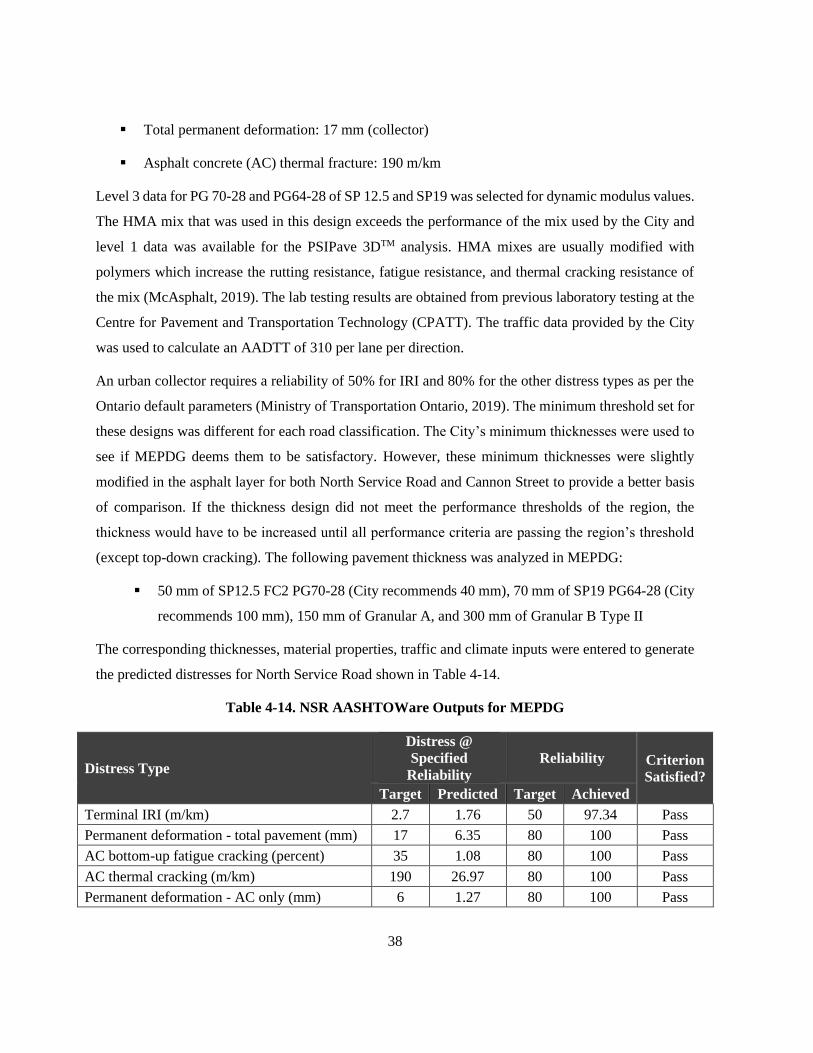
38

▪ Total permanent deformation: 17 mm (collector)

▪ Asphalt concrete (AC) thermal fracture: 190 m/km

Level 3 data for PG 70-28 and PG64-28 of SP 12.5 and SP19 was selected for dynamic modulus values.

The HMA mix that was used in this design exceeds the performance of the mix used by the City and

level 1 data was available for the PSIPave 3DTM analysis. HMA mixes are usually modified with

polymers which increase the rutting resistance, fatigue resistance, and thermal cracking resistance of

the mix (McAsphalt, 2019). The lab testing results are obtained from previous laboratory testing at the

Centre for Pavement and Transportation Technology (CPATT). The traffic data provided by the City

was used to calculate an AADTT of 310 per lane per direction.

An urban collector requires a reliability of 50% for IRI and 80% for the other distress types as per the

Ontario default parameters (Ministry of Transportation Ontario, 2019). The minimum threshold set for

these designs was different for each road classification. The City’s minimum thicknesses were used to

see if MEPDG deems them to be satisfactory. However, these minimum thicknesses were slightly

modified in the asphalt layer for both North Service Road and Cannon Street to provide a better basis

of comparison. If the thickness design did not meet the performance thresholds of the region, the

thickness would have to be increased until all performance criteria are passing the region’s threshold

(except top-down cracking). The following pavement thickness was analyzed in MEPDG:

▪ 50 mm of SP12.5 FC2 PG70-28 (City recommends 40 mm), 70 mm of SP19 PG64-28 (City

recommends 100 mm), 150 mm of Granular A, and 300 mm of Granular B Type II

The corresponding thicknesses, material properties, traffic and climate inputs were entered to generate

the predicted distresses for North Service Road shown in Table 4-14.

Table 4-14. NSR AASHTOWare Outputs for MEPDG

Distress Type

Distress @

Specified

Reliability

Reliability Criterion

Satisfied?

Target Predicted Target Achieved

Terminal IRI (m/km) 2.7 1.76 50 97.34 Pass

Permanent deformation - total pavement (mm) 17 6.35 80 100 Pass

AC bottom-up fatigue cracking (percent) 35 1.08 80 100 Pass

AC thermal cracking (m/km) 190 26.97 80 100 Pass

Permanent deformation - AC only (mm) 6 1.27 80 100 Pass

39

MEPDG deems the tested pavement structure to be sufficient with an achieved reliability of 97.8% in

terminal IRI and 100% in other distress types with the conditions of North Service Road. Top-down

cracking is neglected from the distress types because its failure mechanism is still not fully understood

(Yuan & Warren Lee, 2017). As such, the performance model in MEPDG for top-down cracking is still

undergoing development.

This design’s total thickness is 570 mm and since the silty clay subgrade under the North Service Road

is highly susceptible to frost, this design may not be enough to protect against frost damage. For the

sake of comparison, this pavement structure will be used. The MEPDG output charts can also show the

accumulation of damage over time.


Inputs that change in the design for Cannon Street in the MEPDG design are AADTT, traffic

distribution, HMA mixes, and growth rate. The traffic data provided by the City was used to calculate

an AADTT of 220 per lane per direction.

The growth rate and traffic distribution for Cannon Street were already determined in Section 4.1.1.2.

Using these inputs and the same minimum thickness as per the City’s guidelines, Table 4-15 shows the

predicted distresses for Cannon Street.

▪ 50 mm SP12.5 PG 58-28 (City recommends 40 mm), 70 mm SP12.5 PG 64-28 (City

recommends 100 mm), 150 mm Granular A, and 300 mm Granular B Type II

Table 4-15: CS AASHTOWare Outputs for MEPDG

Distress Type

Distress @

Specified

Reliability


Satisfied?







MEPDG deems the following pavement structure to be sufficient with an achieved reliability of 98.6%

40

in terminal IRI and 100% in other distress types with the conditions of Cannon Street The total

pavement thickness is also 570 mm like North Service Road.


Ontario uses the following performance threshold parameters for an MEPDG design (arterial):

▪ Initial International Roughness Index (IRI): 1 m/km (new asphalt concrete)

▪ Terminal IRI: 2.3 m/km (arterial)

▪ Top-down fatigue cracking: 380 m/km

▪ Bottom-up fatigue cracking: 20% (arterial)

▪ Total permanent deformation: 13 mm (arterial)

▪ Asphalt concrete (AC) thermal fracture: 190 m/km

Other than the performance thresholds, AADTT, growth rate, HMA mixes, traffic distribution, and the

design reliability were the different factors for Stone Church Road. The traffic data provided by the

City was used to calculate an AADTT of 340 per lane per direction. MEPDG recommends a reliability

of 90% for minor arterials (50% for IRI). Therefore, MEPDG recommends the following structure:

▪ 50 mm SP 12.5 FC1 PG64-28, 110 mm SP 19 PG64-28, 150 mm Granular A, and 450 mm

Granular B Type II

This pavement structure achieves the following reliability values.

Table 4-16: SCR AASHTOWare Outputs for MEPDG

Distress Type

Distress @

Specified

Reliability


Satisfied?







MEPDG also deems this structure to be sufficient with an achieved reliability of 89.33% in IRI and

100% in other distresses so this will be selected as the MEPDG thickness design for Stone Church

41

Road. This design is 760 mm in thickness and is adequate for frost. This pavement structure will be

used for comparison.

4.2 PSIPave 3DTM Analysis

The pavement structures obtained from the conventional pavement design methods will be analyzed in

PSIPave 3DTM to check the impact of road geometry, tire types, and bus configurations. North Service

Road thicknesses will be used to assess the impact of geometry, Cannon Street thicknesses will be used

to check the impact of different tire types, and Stone Church Road will be used to assess the impact of

different bus configurations.

North Service Road

A total of twelve cases were chosen for North Service Road designs to evaluate the impact of geometry

on the strains and design life of the pavement. These cases are explained in the next section.

4.2.1.1 Geometry

The LIDAR sensor attached to the PSIPave van provided data about the geometry of North Service

Road. The side slope, surface slope, road width, and ditch depth values were taken from the LIDAR

data. The shoulder widths were taken from Google Earth (Google, 2020). The shoulder widths on the

north and south side of North Service Road are shown in Appendix B. North Service Road is classified

as an urban collector, but the road’s cross section will be determined as rural for design purposes.

The south shoulder width remains consistent throughout the whole road whereas the north shoulder

width changes. The inconsistency in the north side is due to the change in the cross section from urban

to rural (curbs to ditches). The side slopes attained from the LIDAR are shown in Appendix B.

Based on this data, the following geometric conditions were observed on the north side:

▪ Average road width of 3.75 m.

▪ Average side slope of 1:3.8 (1 m height and 3.8 m horizontal length).

▪ Average ditch depth of 1.5 m.

▪ Weighted average shoulder width of 2.2 m.

▪ Average surface slope of -2.3% (the negative implies that it slopes downward from the center

of the road towards the ditches).

Four geometric scenarios (1, 2, 3, and 4) were developed for the analysis based on this summary:

1. 0.7 m shoulder width, 1:1.7 side slope (narrow shoulder, steep side slope).

2. 0.7 m shoulder width, 1:6.4 side slope (narrow shoulder, gradual side slope).

42

3. 3.95 m shoulder width, 1:1.7 side slope (wide shoulder, steep side slope).

4. 3.95 m shoulder width, 1:6.4 side slope (wide shoulder, gradual side slope).

For these cases, the surface slope, road width, and ditch depth were kept constant at -2.3%, 3.5 m, and

1 m, respectively. These values were also mirrored on the south side for symmetry. Figure 4-1 shows

a geometric case in PSIPave 3DTM.

Figure 4-1 PSIPave 3DTM North Service Road Geometry

4.2.1.2 Layers Thicknesses and Material Properties

The thicknesses used were the ones derived from the conventional methods shown below with

AASHTO 93, Shell, and MEPDG classified as Case A, B, and C, respectively shown in Table 4-17.

The asphalt layers were broken down based on constructability reasons.

Table 4-17: Final Designs for NSR

Road Section Design Method

Design Thicknesses (mm)

HMA

Surface

HMA

Binder

Granular

A

Granular

B

North Service

Road

AASHTO 93 (Case A) 60 80 150 450

Shell (Case B) 60 75 260 340

MEPDG (Case C) 50 70 150 300

43

The properties of the layers are shown below, from left to right (modulus of each layer, Poisson’s ratio):

▪ SP12.5 FC2 PG70-28P (Surface): 6934 MPa, 0.35

▪ SP19 PG64-28P (Binder): 11089 MPa, 0.35

▪ Granular A (Base): 250 MPa, 0.35

▪ Granular B Type II (Subbase): 200 MPa, 0.35

▪ Silty Clay (Subgrade): 25 MPa, 0.45

The unit weight for SP12.5 and SP19 was 2530 kgf/m3 and 2460 kgf/m3, respectively. The Poisson’s

ratio and the unit weights were taken from the Ontario parameters for the MEPDG document (Ministry

of Transportation Ontario, 2019).

4.2.1.3 Loading

The vehicle loading, configuration, tire pressure, and maximum load per axle can be defined in PSIPave

3DTM. For the North Service Road section, the truck chosen was a tractor-b train double trailer, labelled

as a category 13 (a seven or more axle, multi-trailer truck) by the FHWA shown in Figure 4-2. The

truck that was chosen for this road section has the highest load equivalency factor (LEF) which has

adverse affects on the pavement (Holguín-Veras, 2010). The maximum load per axle was calculated

based on the Ontario regulation 413/05 (Government of Ontario, 2019).

Figure 4-2 NSR PSIPave 3DTM B-Train Loading Input

44

The load per axle is shown below in Table 4-18:

Table 4-18: Load per Axle for North Service Road

Axle Steer Drive Trailer 1 Trailer 2

Load/Axle

(kg) 5,000 10,300 15,450 15,450

Cannon Street

A total of six cases were chosen for Cannon Street to evaluate the impact of traditional dual tires

versus new generation wide-base tires on the strains and design life of the pavement shown in Figure

4-3. Super singles have been shown to provide economic benefits to the trucking industry, but due to

a higher tire pressure, they cause more fatigue damage in the pavement structure (Al-Qadi & Wang,

2009). In the super single tire case, the steer axle will still use the 11R22.5 tires. The pressure,

diameter, and tire widths used for the analysis are listed below, respectively:

11R22.5 (Conventional Dual Tires): 720 kPa, 1044 mm, 290 mm

455/55R22.5 (Super-Single Tires): 900 kPa, 1064 mm, 460 mm

a) 11R22.5 b) 455/55R22.5

Figure 4-3: Tire Types (OTRUSA, 2020)

4.2.2.1 Geometry

Since Cannon Street has an urban cross section, side slopes will be replaced with sidewalks. The

following geometric scenario was used for this analysis and kept consistent throughout the cases (on

both sides of the road):

45

1) Number of Lanes: 3

Road Width: 3.5 m

Shoulder Width: 1.2 m

Sidewalk Width: 1.9 m

The lane width used was based on the maximum lane width dimension from City of Toronto’s “Road

Engineering Design Guidelines” (City of Toronto, 2017). The shoulder width and sidewalk width

were taken from Google Earth (Google, 2020).


The thicknesses used to parametrize the numerical analysis are shown in Table 4-19.

Table 4-19: Final Designs for CS



HMA

Surface

HMA

Binder

Granular

A

Granular

B

Cannon Street

AASHTO 93 (Case A) 50 80 150 400

Shell (Case B) 50 75 270 330

MEPDG (Case C) 50 70 150 300


▪ SP12.5 PG58-28 (Surface): 7249 MPa, 0.35

▪ SP19 PG64-28 (Binder): 9436 MPa, 0.35




The unit weight for the SP12.5 and SP19 was 2460 kgf/m3. The modulus, Poisson’s ratio and the unit

weights were taken from the Ontario parameters for the MEPDG document (Ministry of Transportation

Ontario, 2019).

4.2.2.3 Loading

The loading used to assess these tire types is a tractor-trailer combination with six axles shown in Figure

4-4.

46

Figure 4-4: NSR PSIPave 3DTM Tractor-Trailer Loading Input

The maximum load per axle and spacings were according to Ontario regulation 413/05 (Government

of Ontario, 2019). As we transition from the traditional dual tires to super singles, the maximum weight

on the drive and trailer axle will increase. However, the loading for both cases were kept the same to

show the impact of tire types. The load per axle is shown below in Table 4-20:

Table 4-20: Load per Axle for Cannon Street

Axle Steer Drive Trailer

Load/Axle

(kg) 5,000 10,900 16,350

Stone Church Road

Since Stone Church Road has the highest bus percentage, a total of nine cases were chosen for Stone

Church Road designs to evaluate the impact of three bus configurations on the strains and design life

of the pavement shown in Figure 4-5. The first bus includes single axles and single tires as shown in

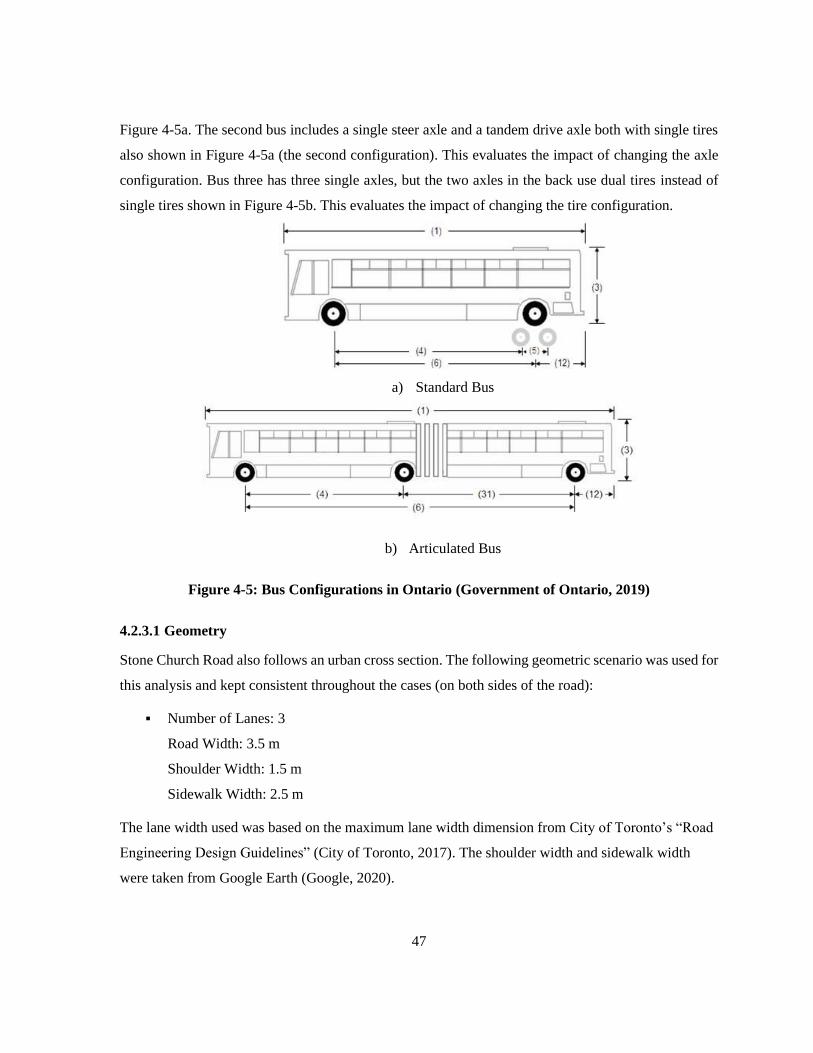
47

Figure 4-5a. The second bus includes a single steer axle and a tandem drive axle both with single tires

also shown in Figure 4-5a (the second configuration). This evaluates the impact of changing the axle

configuration. Bus three has three single axles, but the two axles in the back use dual tires instead of

single tires shown in Figure 4-5b. This evaluates the impact of changing the tire configuration.

a) Standard Bus

b) Articulated Bus

Figure 4-5: Bus Configurations in Ontario (Government of Ontario, 2019)

4.2.3.1 Geometry

Stone Church Road also follows an urban cross section. The following geometric scenario was used for

this analysis and kept consistent throughout the cases (on both sides of the road):

▪ Number of Lanes: 3

Road Width: 3.5 m

Shoulder Width: 1.5 m

Sidewalk Width: 2.5 m

The lane width used was based on the maximum lane width dimension from City of Toronto’s “Road

Engineering Design Guidelines” (City of Toronto, 2017). The shoulder width and sidewalk width

were taken from Google Earth (Google, 2020).

48


The thicknesses used are shown in Table 4-21.

Table 4-21: Final Designs for SCR



HMA

Surface

HMA

Binder

Granular

A

Granular

B

Stone Church

Road

AASHTO 93 (Case A) 60 80 150 400

Shell (Case B) 60 80 260 340

MEPDG (Case C) 50 110 150 450


▪ SP12.5 FC1 PG64-28 (Surface): 4124 MPa, 0.35

▪ SP19 PG64-28 (Binder): 5930 MPa, 0.35




The unit weight for the SP12.5 and SP19 was 2530 kgf/m3 and 2460 kgf/m3, respectively. The dynamic

moduli values used for this case is lower than the other cases. This is due to a lower operating speed of

buses and a lot of stop-and-go conditions which results in a lower frequency. Consequently, the HMA

has a lower dynamic modulus since it behaves more viscously under slower traffic (Harnaeni et al.,

2020). The modulus, Poisson’s ratio and the unit weights were taken from the Ontario parameters for

the MEPDG document (Ministry of Transportation Ontario, 2019).

4.2.3.3 Loading

The bus loads on the pavement structures were already shown in Figure 4-5. The maximum load per

axle and spacings were according to the Ontario regulation 413/05 (Government of Ontario, 2019). As

the axle is changed from single to tandem (Bus 1 to 2) and tires are changed from single to dual (Bus 1

to 3), the maximum load the axle can take is increased, but for these cases the loads were kept the same

to solely evaluate the impact of configuration. Each configuration is shown in Figure 4-6 to Figure 4-8.

49

Figure 4-6: SCR PSIPave 3DTM Bus 1 Configuration



The load per axle is shown below in Table 4-22:

50

Table 4-22: Load per Axle for Stone Church Road

Axle Scenario Steer Drive Trailer

Load/Axle

(kg)

1 5,000 6,400 N/A

2 5,000 6,400 N/A

3 5,000 6,400 6,400

Steer Axle: 5,000 kg, Drive Axle: 6,400 kg, Trailer Axle: 6,400 kg (articulated bus)

51

Chapter 5

RESULTS AND DISCUSSIONS

This chapter presents the results from PSIPave 3DTM for the three road sections and discussed here.

5.1 Impact of Road Geometry

This section is based on the following conference publication: Forghani, F., Tighe, S., Henderson, V.,

Becke, M., Soares, R., & Haichert, R. (2020). Impact of Road Geometry and Thickness on Pavement

Behaviour using PSIPave 3D™. Transportation Association of Canada. The discussions were slightly

modified to respect the flow of the thesis.

North Service Road pavement design thicknesses obtained from AASHTO 93, Shell, and MEPDG were

ran in PSIPave 3DTM to check the impact of road geometry on the normal and shear strains. The

thickness and loading summary for North Service Road is shown in Table 5-1.

Table 5-1: North Service Road Thickness and Load Summary

Thickness (mm) Design Method HMA

Surface

HMA

Binder

Granular

A

Granular

B

North Service Road

AASHTO 93 (Case

A) 60 80 150 450

Shell (Case B) 60 75 260 340

MEPDG (Case C) 50 70 150 300

Loading Truck Type Steer Drive Trailer 1 Trailer 2

Load Per Axle (kg) B-Train 5,000 10,300 15,450 15,450

PSIPave 3D™ Normal Strains

The peak tensile strain in the direction of traffic in the asphalt binder layer expresses the strain caused

by traffic which leads to fatigue failure (bottom-up cracking). This type of failure initiates in the bottom

of the deepest asphalt layer and propagates upwards. The peak tensile strain measured in the asphalt

binder for each case is shown in Figure 5-1.

52

Figure 5-1: NSR Peak Tensile Strain in Asphalt Binder (μm/m)

Based on these findings, the following observations were made within the peak tensile strain results:

▪ The tensile strains observed in the MEPDG design are on average 24% more than AASHTO

93 and 22% more than Shell. This is likely because of the thickness difference in the asphalt

layers and entire pavement structure. The MEPDG design has only 86 % of the asphalt layer

thickness of AASHTO 93 and 89 % of Shell. The asphalt difference in thickness is 5 mm

between AASHTO 93 and Shell design and 20 mm between AASHTO 93 and MEPDG design.

▪ Overall, the geometry has minimal effects on the tensile strains, though it seems to have more

of an impact in MEPDG where the total pavement thickness is lower.

▪ The area under the steer axle experienced the greatest tensile strain in each case. This is due to

higher contact pressures under the steer axle. The other axles (tandem and tridem) have dual

tires which distribute the strains across a larger footprint.

The peak compressive strain in the subgrade is shown in Figure 5-2. This value describes the tendency

for rutting in the subgrade due to loading. When the subgrade deforms, the whole pavement structure

sitting on the subgrade also settles and leads to poor performance overall.

80

80 81

81 8

5

84 86

84

10

3

10

1

99 1

04

63

61 62

61 62

62 63

62

76

76

75

75

62

61

61

60 61

61

60 61

78

75 77

77

62

60 61

60 61

61

61

61

75

75

75

73

0

20

40

60

80

100

120

1.7:1 6.4:1 1.7:1 6.4:1 1.7:1 6.4:1 1.7:1 6.4:1 1.7:1 6.4:1 1.7:1 6.4:1

0.7m Shoulder 3.95m Shoulder 0.7m Shoulder 3.95m Shoulder 0.7m Shoulder 3.95m Shoulder

AASHTO Shell MEPDG

Asp

hal

t B

ind

er

Co

urs

e -

Pe

ak T

en

sile

St

rain

(μ

m/m

)

Steer Drive Tridem1 Tridem2

53

Figure 5-2: NSR Peak Compressive Strain in Subgrade (μm/m)

Based on these cases, the following observations were made within the peak compressive strain results:

▪ The compressive strains observed in MEPDG are on average 23% more than AASHTO 93 and

21% more than Shell.

o The AASHTO 93 design is only 5 mm thicker than the Shell design, and this difference

is in the asphalt layer.

o The distribution of granular material layer thicknesses differs between the AASHTO

93 and Shell design but both the base and subbase granular are similar quality material.

o Shell has a thicker base granular layer which has slightly better properties than the

subbase.

o The effects of geometry were minimal on the peak compressive strains though it seems

to have more of an impact in the MEPDG design where the pavement structure is

thinner.

▪ Even though the effect is minimal, the peak compressive strains are slightly reduced as the

transition is made from narrow to wide shoulders.

PSIPave 3D™ Shear Strains

Shear strain is a common mechanism of failure of pavement structures; however, this parameter is not

frequently analyzed due to the requirement to utilize three-dimensional modeling to accurately quantify

the behaviour. Given the capability of PSIPave 3D™ to provide this information, the peak shear strains

13

7

13

3

13

0

13

3

14

0

14

0

13

7

13

9

18

7

18

1

17

7

18

1

18

7

18

5

18

2

18

4

19

0

18

8

18

4

18

5

23

0

22

8

22

2

22

2

22

4

22

5

22

2

22

1

22

8

22

5

22

1

22

2

26

9

26

9

26

3

26

3

22

7

22

6

22

2

22

4

23

1

22

8

22

5

22

5

27

2

27

2

26

9

26

7

0

50

100

150

200

250

300

1.7:1 6.4:1 1.7:1 6.4:1 1.7:1 6.4:1 1.7:1 6.4:1 1.7:1 6.4:1 1.7:1 6.4:1


AASHTO Shell MEPDG

Sub

grad

e -

Pe

ak C

om

pre

ssiv

e S

trai

n

(μm

/m)


54

in the asphalt top course, subbase, subgrade and subgrade side slope are shown in Figure 5-3 to Figure

5-5. Shear distributions and peaks across all planes, layers, and lanes were determined but the following

figures only show the peak shear strains in the YZ direction.

Figure 5-3: NSR Peak Shear Strain in Asphalt Top Course (μm/m)

Figure 5-4: NSR Peak Shear Strain in Granular Subbase (μm/m)

12

0

12

1

12

0

12

2

12

3

12

3

12

2

12

3 14

0

13

8

13

8

13

9

10

2

10

4

10

2

10

4

10

4

10

1

10

4

10

7

10

5 11

1

11

0

10

8

10

2

10

6

10

2

10

4

10

7

10

4

10

6

10

3 10

9

10

7

10

5

10

6

10

3

10

8

10

5

10

3

10

4

10

6

10

5

10

3

10

8

11

0

10

6

11

0

0

20

40

60

80

100

120

140

160

1.7:1 6.4:1 1.7:1 6.4:1 1.7:1 6.4:1 1.7:1 6.4:1 1.7:1 6.4:1 1.7:1 6.4:1


AASHTO Shell MEPDG

Asp

hal

t To

p C

ou

rse

-P

eak

Sh

ear

Str

ain

(μ

m/m

)


10

2

10

3

10

0

10

2

81 82 83

82

12

6

13

1

13

0

12

613

6

13

6

13

9

13

6

11

9

11

5

11

2

11

3

15

0

15

1

14

4

14

5

14

2

14

0

14

0

13

8

11

6

11

8

11

9

11

7

15

3 16

0

15

6

15

3

15

0

14

3

14

5

14

6

12

3

12

0

12

4

12

0

15

1

15

6

15

7

15

3

0

20

40

60

80

100

120

140

160

180

1.7:1 6.4:1 1.7:1 6.4:1 1.7:1 6.4:1 1.7:1 6.4:1 1.7:1 6.4:1 1.7:1 6.4:1


AASHTO Shell MEPDG

Sub

bas

e -

Pe

ak S

he

ar S

trai

n (μ

m/m

)


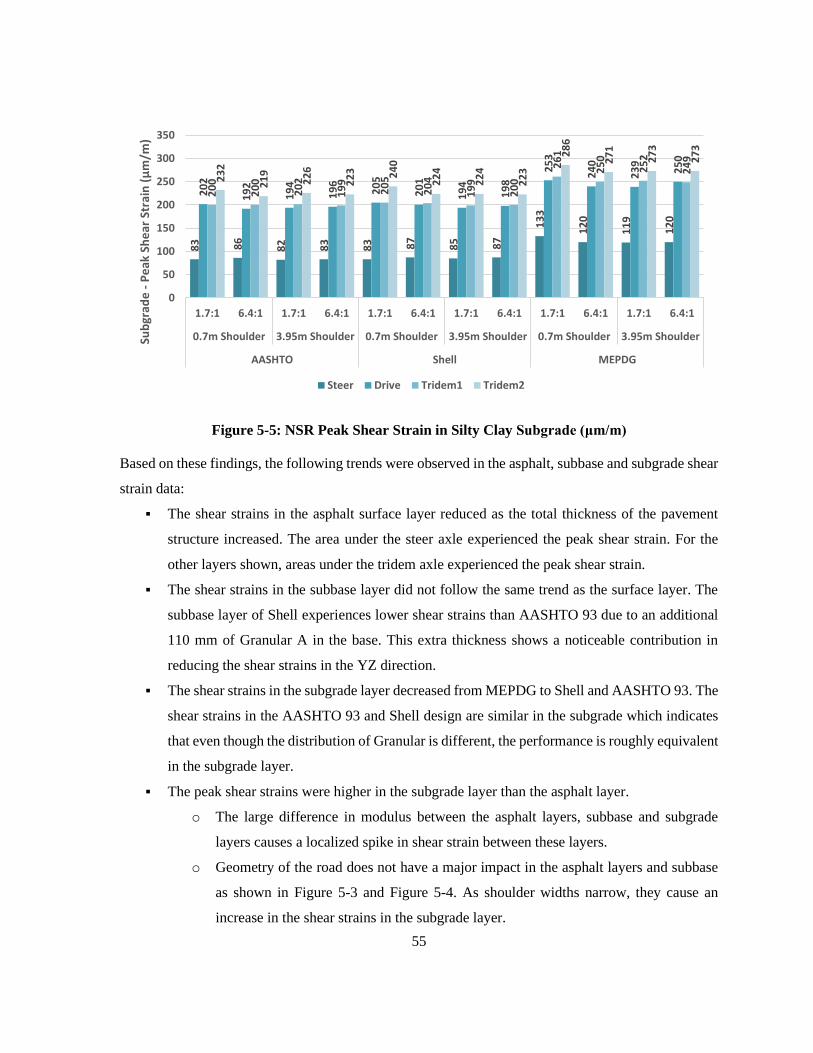
55

Figure 5-5: NSR Peak Shear Strain in Silty Clay Subgrade (μm/m)

Based on these findings, the following trends were observed in the asphalt, subbase and subgrade shear

strain data:

▪ The shear strains in the asphalt surface layer reduced as the total thickness of the pavement

structure increased. The area under the steer axle experienced the peak shear strain. For the

other layers shown, areas under the tridem axle experienced the peak shear strain.

▪ The shear strains in the subbase layer did not follow the same trend as the surface layer. The

subbase layer of Shell experiences lower shear strains than AASHTO 93 due to an additional

110 mm of Granular A in the base. This extra thickness shows a noticeable contribution in

reducing the shear strains in the YZ direction.

▪ The shear strains in the subgrade layer decreased from MEPDG to Shell and AASHTO 93. The

shear strains in the AASHTO 93 and Shell design are similar in the subgrade which indicates

that even though the distribution of Granular is different, the performance is roughly equivalent

in the subgrade layer.

▪ The peak shear strains were higher in the subgrade layer than the asphalt layer.

o The large difference in modulus between the asphalt layers, subbase and subgrade

layers causes a localized spike in shear strain between these layers.

o Geometry of the road does not have a major impact in the asphalt layers and subbase

as shown in Figure 5-3 and Figure 5-4. As shoulder widths narrow, they cause an

increase in the shear strains in the subgrade layer.

83 86

82 83

83 87

85 87

13

3

12

0

11

9

12

0

20

2

19

2

19

4

19

6

20

5

20

1

19

4

19

8

25

3

24

0

23

9

25

0

20

0

20

0

20

2

19

9

20

5

20

4

19

9

20

0

26

1

25

0

25

2

24

9

23

2

21

9

22

6

22

3 24

0

22

4

22

4

22

3

28

6

27

1

27

3

27

3

0

50

100

150

200

250

300

350

1.7:1 6.4:1 1.7:1 6.4:1 1.7:1 6.4:1 1.7:1 6.4:1 1.7:1 6.4:1 1.7:1 6.4:1


AASHTO Shell MEPDG

Sub

grad

e -

Pe

ak S

he

ar S

trai

n (μ

m/m

)


56

o The shear strains are increased as the slopes are steeper for the narrow shoulder width

(0.7 m). This is most evident in the MEPDG design.

5.1.2.1 Shear Strains in the Side Slope

Two examples of the contours generated by the 12 cases are presented in Figure 5-6 and Figure 5-7.

Figure 5-6: NSR Shear Strain Contour for AASHTO 93 Thicknesses, 3.95 m Shoulder, 6.4:1

Side Slope

57

Figure 5-7: NSR Shear Strain Contour for MEPDG Thicknesses, 0.7 m Shoulder, 1.7:1 Side

Slope

The three-dimensional contours shown in these figures highlight the shear strains in the pavement under

traffic loading. The cross section shown is located beneath the tridem load. The contour scale goes from

green (0 μm/m) to red (±71 μm/m).

▪ The case illustrated in Figure 5-6 has the greatest pavement structure thickness, the widest

shoulders, and the gentlest slopes. As shown, the response in the pavement structure is minimal.

▪ In comparison, the case illustrated in Figure 5-7 has the least pavement structure thickness,

narrow shoulders and steep slopes. Higher shear strains were observed under the load for the

MEPDG case because of a thinner pavement structure, but the major difference is shown in the

side slopes. In the case of MEPDG, the shear strains on the side slope are prominent, whereas

in the AASHTO case there is minimal strain.

The response from the pavement structure identifies the effect that road geometry has on pavement

performance and behaviour. The strains experienced in thinner pavement sections are greater and peak

deflections are also greater.

58

The loading from the truck is observed to produce higher shear strains throughout the width of the

loaded lane, in the shoulder and side slope for the thinner/narrower structure. Therefore, additional

investigation of the shear strain in the subgrade side slope was investigated as illustrated in Figure 5-8.

The impact of road geometry is most evident in the subgrade side slope below. The investigation of the

side slope is important as high strains could lead to cracking along the edges of the pavement structure

which eventually can propagate to the traffic lane and cause further issues.

Figure 5-8: NSR Peak Shear Strain in Subgrade Side Slope (μm/m)

The following trends were observed in the subgrade side slope:

▪ The shear strain in the subgrade side slope is dependent on the width of the shoulder and the

side slope.

▪ Comparing the results within the same layer thickness cases, the difference in shear strain

between the narrowest cases (narrow shoulders, steep side slope) and widest cases (wide

shoulder and gradual side slope) increased by 520%, 530% and 550% for the AASHTO 93,

Shell, and MEPDG thickness cases, respectively. PSIPave 3DTM can show the effect of these

factors which other design methods do not account for.

▪ Therefore, geometry has a major effect on the subgrade side slope and these strains can cause

failures in the side slope damaging the integrity of the overall pavement structure. Further

issues such as erosion and entrance of moisture can take place which reduce the pavement

performance. Figure 5-8 shows the importance of building wider shoulders to effectively

reduce the shear strains in these cases.

45

21 3

0

20

49

26

36

20

59

22

33

21

90

76

30

17

91

76

35

17

95

80

28

17

75

74

8 5

75

68

8 5

81

80

8 5

10

6

93

30

19

10

8

89

35

19

11

1

97

32

20

0

20

40

60

80

100

120

1.7:1 6.4:1 1.7:1 6.4:1 1.7:1 6.4:1 1.7:1 6.4:1 1.7:1 6.4:1 1.7:1 6.4:1


AASHTO Shell MEPDG

Sub

grad

e S

ide

slo

pe

-P

eak

Sh

ear

St

rain

(μ

m/m

)


59

Another way to visualize this is to look at the output manager in PSIPave 3DTM which can generate

graphs of the strains on a given plane. Two cases of shear strain in the subgrade side slope are shown

here for comparison in Figure 5-9 and Figure 5-10.

Figure 5-9: NSR Shear Strain for AASHTO 93 Thicknesses, 0.7 m Shoulder, 1.7:1 Side Slope

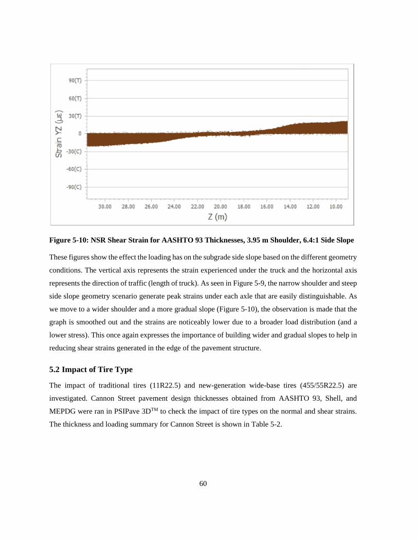
60

Figure 5-10: NSR Shear Strain for AASHTO 93 Thicknesses, 3.95 m Shoulder, 6.4:1 Side Slope

These figures show the effect the loading has on the subgrade side slope based on the different geometry

conditions. The vertical axis represents the strain experienced under the truck and the horizontal axis

represents the direction of traffic (length of truck). As seen in Figure 5-9, the narrow shoulder and steep

side slope geometry scenario generate peak strains under each axle that are easily distinguishable. As

we move to a wider shoulder and a more gradual slope (Figure 5-10), the observation is made that the

graph is smoothed out and the strains are noticeably lower due to a broader load distribution (and a

lower stress). This once again expresses the importance of building wider and gradual slopes to help in

reducing shear strains generated in the edge of the pavement structure.

5.2 Impact of Tire Type

The impact of traditional tires (11R22.5) and new-generation wide-base tires (455/55R22.5) are

investigated. Cannon Street pavement design thicknesses obtained from AASHTO 93, Shell, and

MEPDG were ran in PSIPave 3DTM to check the impact of tire types on the normal and shear strains.

The thickness and loading summary for Cannon Street is shown in Table 5-2.

61

Table 5-2: Cannon Street Thickness and Load Summary


Surface

HMA

Binder

Granular

A

Granular

B

Cannon Street

AASHTO 93 (Case

A) 50 80 150 400

Shell (Case B) 50 75 270 330

MEPDG (Case C) 50 70 150 300

Loading Truck Type Steer Drive Trailer

Load Per Axle (kg) Tractor-Trailer 5,000 10,900 16,350

PSIPave 3D™ Normal Strains

The peak tensile strain measured in the asphalt binder for each case is shown in Figure 5-11. An extra

three cases for Shell were ran because the Shell designs were done with a subgrade modulus of 25 MPa.

The 35 MPa case was also included to make it a consistent comparison between the two other cases.

Figure 5-11: CS Peak Tensile Strain in Asphalt Binder Course (μm/m)


▪ Tensile strains increase with decreasing asphalt thickness (AASHTO 93 to Shell to MEPDG)

o There is almost no change in the tensile strain for the steer axle. That is because the

tire types for both steer axles are 11R22.5. The extra tire pressure in the other axles do

not affect the steer axle.

96

95 98 99

97 10

0 11

0

10

7

75

97

77

10

5

77

10

4

88

11

6

72

97

76

99

76

10

0

85

11

4

0

20

40

60

80

100

120

140

11

R2

2.5

45

5/5

5R

22

.5

11

R2

2.5

45

5/5

5R

22

.5

11

R2

2.5

45

5/5

5R

22

.5

11

R2

2.5

45

5/5

5R

22

.5AASHTO Shell (35 MPa) Shell (25 MPa) MEPDG

Asp

hal

t B

ind

er

Co

urs

e -

Pe

ak T

en

sile

St

rain

(μ

m/m

)

Steer Drive Tridem

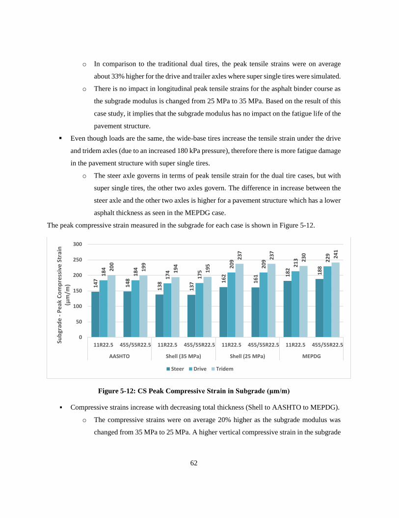
62

o In comparison to the traditional dual tires, the peak tensile strains were on average

about 33% higher for the drive and trailer axles where super single tires were simulated.

o There is no impact in longitudinal peak tensile strains for the asphalt binder course as

the subgrade modulus is changed from 25 MPa to 35 MPa. Based on the result of this

case study, it implies that the subgrade modulus has no impact on the fatigue life of the

pavement structure.

▪ Even though loads are the same, the wide-base tires increase the tensile strain under the drive

and tridem axles (due to an increased 180 kPa pressure), therefore there is more fatigue damage

in the pavement structure with super single tires.

o The steer axle governs in terms of peak tensile strain for the dual tire cases, but with

super single tires, the other two axles govern. The difference in increase between the

steer axle and the other two axles is higher for a pavement structure which has a lower

asphalt thickness as seen in the MEPDG case.

The peak compressive strain measured in the subgrade for each case is shown in Figure 5-12.

Figure 5-12: CS Peak Compressive Strain in Subgrade (μm/m)

▪ Compressive strains increase with decreasing total thickness (Shell to AASHTO to MEPDG).

o The compressive strains were on average 20% higher as the subgrade modulus was

changed from 35 MPa to 25 MPa. A higher vertical compressive strain in the subgrade

14

7

14

8

13

8

13

7 16

2

16

1 18

2

18

8

18

4

18

4

17

4

17

5

20

9

20

9

21

3 22

9

20

0

19

9

19

4

19

5

23

7

23

7

23

0 24

10

50

100

150

200

250

300

11R22.5 455/55R22.5 11R22.5 455/55R22.5 11R22.5 455/55R22.5 11R22.5 455/55R22.5

AASHTO Shell (35 MPa) Shell (25 MPa) MEPDG

Sub

grad

e -

Pe

ak C

om

pre

ssiv

e S

trai

n

(μm

/m)

Steer Drive Tridem

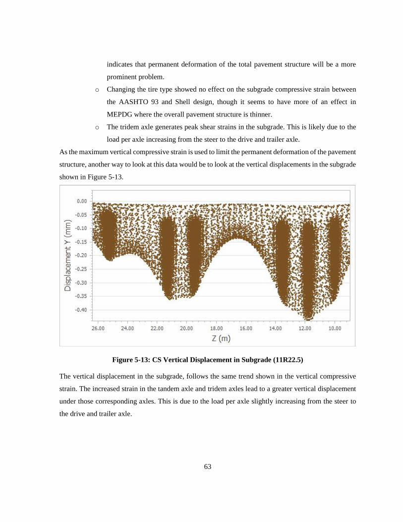
63

indicates that permanent deformation of the total pavement structure will be a more

prominent problem.

o Changing the tire type showed no effect on the subgrade compressive strain between

the AASHTO 93 and Shell design, though it seems to have more of an effect in

MEPDG where the overall pavement structure is thinner.

o The tridem axle generates peak shear strains in the subgrade. This is likely due to the

load per axle increasing from the steer to the drive and trailer axle.

As the maximum vertical compressive strain is used to limit the permanent deformation of the pavement

structure, another way to look at this data would be to look at the vertical displacements in the subgrade

shown in Figure 5-13.

Figure 5-13: CS Vertical Displacement in Subgrade (11R22.5)

The vertical displacement in the subgrade, follows the same trend shown in the vertical compressive

strain. The increased strain in the tandem axle and tridem axles lead to a greater vertical displacement

under those corresponding axles. This is due to the load per axle slightly increasing from the steer to

the drive and trailer axle.

64

PSIPave 3D™ Shear Strains

The peak shear strains in the asphalt top course, subbase and subgrade (in the YZ direction) are

shown in Figure 5-14 to Figure 5-16.

Figure 5-14: CS Peak Shear Strain in Asphalt Top Course (μm/m)

Figure 5-15: CS Peak Shear Strain in Subbase (μm/m)

12

1

12

1 12

7

12

8

12

7

12

8 13

4

13

3

10

2

12

5

10

6

12

9

10

1

12

9

10

3

12

9

99

12

7

10

2

12

8

10

3

12

7

10

6

13

0

0

20

40

60

80

100

120

140

160

11R22.5 455/55R22.5 11R22.5 455/55R22.5 11R22.5 455/55R22.5 11R22.5 455/55R22.5


Asp

hal

t To

p C

ou

rse

-P

eak

Sh

ear

Str

ain

(μ

m/m

)

Steer Drive Tridem

12

3

12

4

92 93

93

92

13

0

13

4

12

8 13

5

10

6

10

6

11

0

11

1

13

5

15

7

13

2 13

8

10

8

10

9

11

3

11

4

13

7 14

7

0

20

40

60

80

100

120

140

160

180

11R22.5 455/55R22.5 11R22.5 455/55R22.5 11R22.5 455/55R22.5 11R22.5 455/55R22.5


Sub

bas

e -

Pe

ak S

he

ar S

trai

n (μ

m/m

)

Steer Drive Tridem

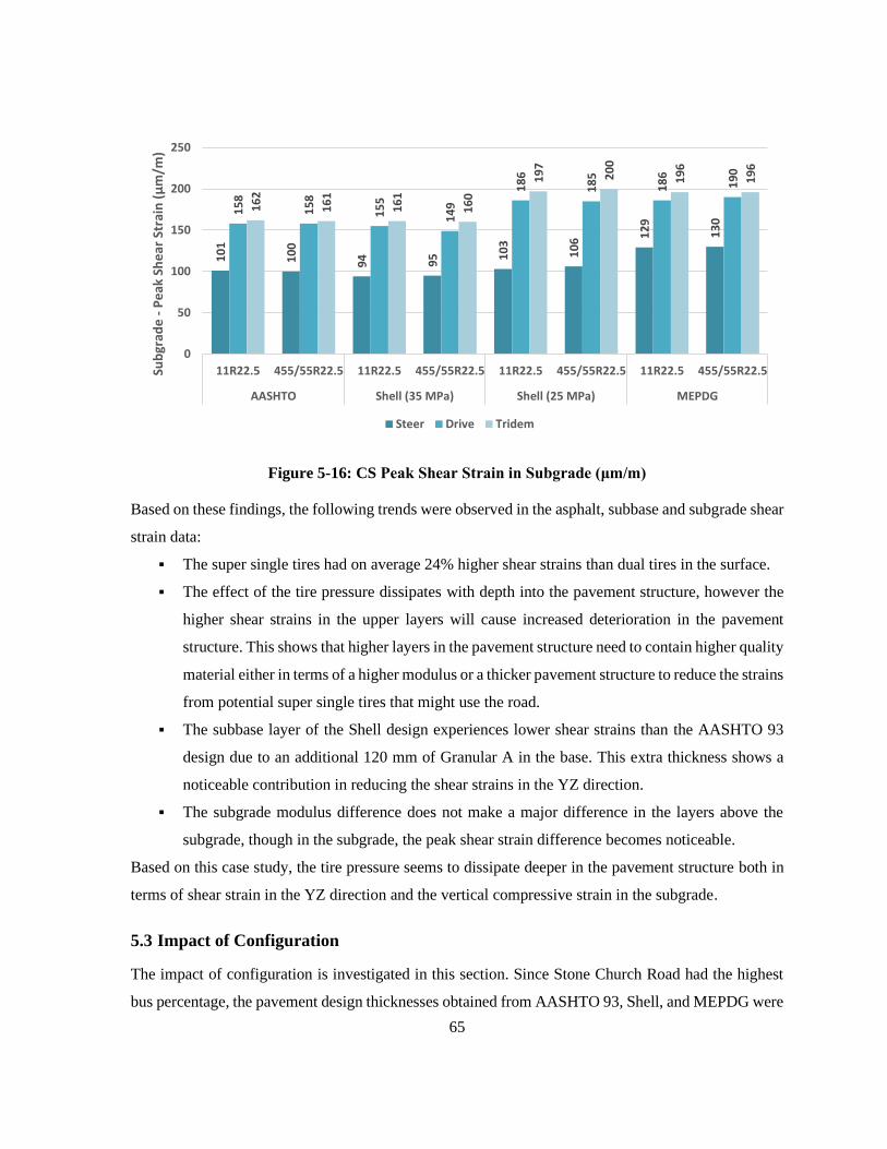
65

Figure 5-16: CS Peak Shear Strain in Subgrade (μm/m)


strain data:

▪ The super single tires had on average 24% higher shear strains than dual tires in the surface.

▪ The effect of the tire pressure dissipates with depth into the pavement structure, however the

higher shear strains in the upper layers will cause increased deterioration in the pavement

structure. This shows that higher layers in the pavement structure need to contain higher quality

material either in terms of a higher modulus or a thicker pavement structure to reduce the strains

from potential super single tires that might use the road.

▪ The subbase layer of the Shell design experiences lower shear strains than the AASHTO 93

design due to an additional 120 mm of Granular A in the base. This extra thickness shows a

noticeable contribution in reducing the shear strains in the YZ direction.

▪ The subgrade modulus difference does not make a major difference in the layers above the

subgrade, though in the subgrade, the peak shear strain difference becomes noticeable.

Based on this case study, the tire pressure seems to dissipate deeper in the pavement structure both in

terms of shear strain in the YZ direction and the vertical compressive strain in the subgrade.

5.3 Impact of Configuration

The impact of configuration is investigated in this section. Since Stone Church Road had the highest

bus percentage, the pavement design thicknesses obtained from AASHTO 93, Shell, and MEPDG were

10

1

10

0

94 95 1

03

10

6 12

9

13

0

15

8

15

8

15

5

14

9

18

6

18

5

18

6

19

0

16

2

16

1

16

1

16

0

19

7

20

0

19

6

19

6

0

50

100

150

200

250

11R22.5 455/55R22.5 11R22.5 455/55R22.5 11R22.5 455/55R22.5 11R22.5 455/55R22.5


Sub

grad

e -

Pe

ak S

he

ar S

trai

n (μ

m/m

)

Steer Drive Tridem

66

run in PSIPave 3DTM to check the impact of bus configurations on the normal and shear strains. The

thickness and loading summary for Stone Church Road is shown in

Table 5-3: Stone Church Road Thickness and Load Summary


Surface

HMA

Binder

Granular

A

Granular

B

Cannon Street

AASHTO 93 (Case

A) 60 80 150 400

Shell (Case B) 60 80 260 340

MEPDG (Case C) 50 110 150 450

Loading Loading Type Steer Drive Trailer

Load Per Axle (kg)

Bus 1 5,000 6,400 N/A

Bus 2 5,000 6,400 N/A

Bus 3 5,000 6,400 6,400

PSIPave 3DTM Normal Strains

The peak tensile strain measured in the asphalt binder for each case is shown in Figure 5-17.

Figure 5-17: SCR Peak Tensile Strain in Asphalt Binder Course (μm/m)


▪ Tensile strains decrease with increasing asphalt thickness (AASHTO 93 to MEPDG)

12

8

13

0

13

1

12

7

13

1

13

1

12

8

13

2

13

1

10

3

10

3

10

4

15

7

87

11

4

15

7

88

11

4

15

8

88

11

5 12

5

66

90

11

3

11

3

11

4

92

0

20

40

60

80

100

120

140

160

180

Bus 1 Bus 2 Bus 3 Bus 1 Bus 2 Bus 3 Bus 1 Bus 2 Bus 3 Bus 1 Bus 2 Bus 3

AASHTO Shell (35 Mpa) Shell (25 Mpa) MEPDG

Asp

hal

t B

ind

er

Co

urs

e -

Pe

ak T

en

sile

St

rain

(μ

m/m

)

Steer Drive Trailer

67

o The longitudinal tensile strains of the AASHTO 93 and Shell design are consistent

which means that the longitudinal tensile strain in the binder course is only dependent

on the thickness of the asphalt course and its modulus. A different subgrade modulus

is not found to make an impact on the fatigue life of the pavement structure.

▪ When comparing single axle to a tandem axle (Bus 1 to Bus 2), the tensile strains are on average

46% less. In the case of single tires, the tandem axle helps distribute the same load over two

axles and four tires instead.

▪ Dual tires on a single axle decreases the tensile strain under that axle, but not as much as the

transition from a single axle to a tandem axle. However, when a tandem axle is used, there will

be two peak tensile strains under that bus. A fatigue analysis is presented in the next section to

evaluate the fatigue damage of these bus types as it is unknown if two passes of 87 microstrain

will cause a greater fatigue damage than one pass of 157 microstrain.

The peak compressive strain measured in the subgrade for each case is shown in Figure 5-18.

Figure 5-18: SCR Peak Compressive Strain in Subgrade (μm/m)

Based on these cases, the following observations were made within the peak compressive strain results:

▪ Compressive strains increase with decreasing total thickness (MEPDG to Shell to AASHTO)

▪ The compressive strain has a similar trend to the tensile strains as we change from Bus 1 to

Bus 2. However, it is observed that the dual tires (compared to single tires) do not cause a major

17

3

17

2

17

3

15

8

15

7

15

7

18

2

18

2

18

1

14

2

14

5

14

5

22

4

13

6

21

9

20

3

12

5

20

1

23

5

15

0

23

6

18

3

11

9

18

3

21

7

20

1

23

4

18

30

50

100

150

200

250


AASHTO Shell (35 Mpa) Shell (25 Mpa) MEPDG

Sub

grad

e -

Pe

ak C

om

pre

ssiv

e S

trai

n

(μm

/m)

Steer Drive Trailer

68

shift in the vertical compressive strains in the subgrade. This is due to the load acting on a

single axle (i.e. the load is not distributed).

o For the subgrade, the drive and trailer axles govern in terms of peak shear strain due to

an increase in vertical loading on that axle. Comparing to a single axle, a tandem axle

decreases the load per axle by half and therefore causes a much lower strain in the drive

axle.

To better visualize the tensile strains, the peak tensile strains under each bus loading is shown in Figure

5-19 to Figure 5-21.

Figure 5-19: SCR Tensile Strain in Asphalt Binder Course (Bus 1)


69


Using the steer axle peak tensile strain as a basis of comparison, it is shown the effect that each

configuration has on the drive and trailer axles in the back of the bus. It is also visually clear from these

figures that the tandem axle has a greater effect in reducing the tensile strains than the dual tire

configuration. The peak tensile strains obtained from the figure above will be used to perform a fatigue

comparison to assess which case will be the most destructive on the pavement structure in terms of

fatigue.

5.3.1.1 Fatigue Comparison

The comparison for fatigue was made based on the number of bus repetitions to fatigue failure. Equation

2-4 was used to calculate the number of allowable fatigue repetitions based on the peak tensile strains

in the asphalt binder course under each axle. The f1, f2, f3 constants used were 0.1001, 3.565, and 1.474

respectively (Behiry, 2012). The tensile strain and modulus used were the peak tensile strains in the

asphalt binder course layer and the corresponding asphalt binder modulus. Table 5-4 shows that the

allowable fatigue cycles in the steer axle do not change in each scenario which is reasonable as the load

or configuration of that axle is not being changed. However, comparing Bus 1 to Bus 2 identifies a 46%

drop in tensile strain which increases the allowable number of fatigue cycles by a factor of 8, while

comparing Bus 1 to Bus 3 only increases the allowable number by a factor of 3. FHWA fatigue

constants were used to calculate the allowable number of fatigue repetitions (Behiry, 2012).

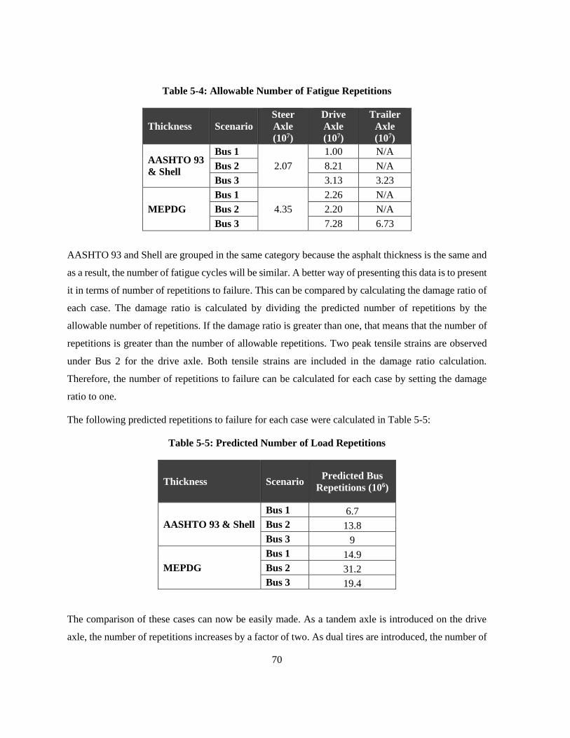
70

Table 5-4: Allowable Number of Fatigue Repetitions

Thickness Scenario

Steer

Axle

(107)

Drive

Axle

(107)

Trailer

Axle

(107)

AASHTO 93

& Shell

Bus 1

2.07

1.00 N/A

Bus 2 8.21 N/A

Bus 3 3.13 3.23

MEPDG

Bus 1

4.35

2.26 N/A

Bus 2 2.20 N/A

Bus 3 7.28 6.73

AASHTO 93 and Shell are grouped in the same category because the asphalt thickness is the same and

as a result, the number of fatigue cycles will be similar. A better way of presenting this data is to present

it in terms of number of repetitions to failure. This can be compared by calculating the damage ratio of

each case. The damage ratio is calculated by dividing the predicted number of repetitions by the

allowable number of repetitions. If the damage ratio is greater than one, that means that the number of

repetitions is greater than the number of allowable repetitions. Two peak tensile strains are observed

under Bus 2 for the drive axle. Both tensile strains are included in the damage ratio calculation.

Therefore, the number of repetitions to failure can be calculated for each case by setting the damage

ratio to one.

The following predicted repetitions to failure for each case were calculated in Table 5-5:

Table 5-5: Predicted Number of Load Repetitions

Thickness Scenario Predicted Bus

Repetitions (106)

AASHTO 93 & Shell

Bus 1 6.7

Bus 2 13.8

Bus 3 9

MEPDG

Bus 1 14.9

Bus 2 31.2

Bus 3 19.4

The comparison of these cases can now be easily made. As a tandem axle is introduced on the drive

axle, the number of repetitions increases by a factor of two. As dual tires are introduced, the number of

71

repetitions increases by a factor of 1.34 even considering that the gross load of Bus 3 is 6400 kg higher.

These results express the impact vehicle configuration has on the fatigue life of the pavement structure.

Single axle and single tires noticeably reduce the fatigue life.

There is a similar trend in the MEPDG case for the number of repetitions as the configuration is

changed. However, another conclusion that can be derived from these values is the value of adding the

extra 20 mm of asphalt thickness. The conclusion made earlier about fatigue life being dependent on

asphalt thickness is also shown here. The number of repetitions is over 2 times in comparison to

AASHTO 93 and Shell.

PSIPave 3DTM Shear Strains

The peak shear strains in the asphalt top course, subbase and subgrade (in the YZ direction) are

shown in Figure 5-22 to Figure 5-25.

Figure 5-22: SCR Peak Shear Strain in Asphalt Top Course (μm/m)

21

6

21

6

21

8

22

2

21

9

21

6

21

9

21

9

21

9

20

6

20

5

20

2

23

4

19

7

20

2

24

2

20

6

20

6 23

4

20

6

20

6

21

2

19

1

19

620

8

19

7

19

7

18

4

0

50

100

150

200

250

300



Asp

hal

t Su

rfac

e C

ou

rse

-P

eak

Sh

ear

St

rain

(μ

m/m

)

Steer Drive Trailer

72

Figure 5-23: SCR Peak Shear Strain in Base (μm/m)

Figure 5-24: SCR Peak Shear Strain in Subbase (μm/m)

25

0

24

8

24

3

25

2

25

0

24

0 25

4

25

2

24

3

20

0

19

3

19

6

31

7

17

3 20

2

31

7

17

6 20

7

32

0

17

5

21

1

25

0

13

4 16

5

20

5

19

6 21

2

16

7

0

50

100

150

200

250

300

350



Bas

e -

Pe

ak S

hea

r St

rain

(μ

m/m

)

Steer Drive Trailer

14

3

14

6

14

5

10

7

10

1

10

1 11

0

10

3

10

4 11

7

12

2

12

2

17

9

10

5

15

9

13

3

79

12

6 13

9

83

13

1 14

6

92

13

2

16

0

12

5

12

9 13

70

20

40

60

80

100

120

140

160

180

200



Sub

bas

e -

Pe

ak S

he

ar S

trai

n (μ

m/m

)

Steer Drive Trailer

73

Figure 5-25: SCR Peak Shear Strain in Subgrade (μm/m)


strain data:

▪ Increasing total asphalt thickness decreases the peak shear strains in the asphalt top course.

o The peak shear strain in the steer axle is dependent on the weight on that axle rather

than the gross weight of bus as there is very minor change throughout the different

cases.

o Above the base, AASHTO 93 and Shell have similar structures so there is minimal

difference in the strains.

o MEPDG has the lowest strains in the base because its overall asphalt thickness is 20

mm thicker. This 20 mm extra thickness shows a noticeable contribution in reducing

the shear strains in the YZ direction.

o Shell has lower strains in the subbase due to a 110 mm thicker Granular in the base

which is even lower than MEPDG.

▪ The peak shear strains are decreased from Bus 1 to Bus 2.

o Changing the configuration from Bus 1 to Bus 3 reduces the peak shear strains in all

the layers except the subgrade.

o Changing the configuration from Bus 2 to Bus 3 increases the peak shear strains in all

the layers. This shows that the effect of changing to a tandem axle is much greater than

switching from single to dual tires in reducing the peak shear strains.

12

3

11

8

12

0

11

5

10

5 11

5 13

0

12

4 13

1

10

1

10

4

10

8

15

2

11

4

15

4

13

4

10

3

14

3 15

7

12

0

16

2

12

8

98

13

6

15

7

14

8 16

6

13

6

0

20

40

60

80

100

120

140

160

180



Sub

grad

e -

Pe

ak S

he

ar S

trai

n (μ

m/m

)

Steer Drive Trailer

74

Chapter 6

CONCLUSION

To date, pavement design is still undergoing development. Conventional methods have been used in

the field with success to develop pavement structures. Each pavement design method discussed in this

research has benefits. For example, AASHTO 93 and Shell can determine the required thickness for a

pavement structure. MEPDG can analyze a pavement design to predict the accumulation of damage

throughout the design life. One of the ways to advance pavement design further is to see what impacts

climate, road geometry, tire types, and different bus configurations have on the pavement behavior.

None of the techniques investigated here account for shear strain which is a common mechanism of

failure of pavement structures. This parameter is not frequently analyzed due to the requirement to

utilize three-dimensional modeling to accurately quantify the behaviour. In this research, three road

sections were chosen in the City of Hamilton to analyze the impact of road geometry, tire types, and

bus configurations on the normal and shear strains. Based on a case study undertaken in the City of

Hamilton, the following observations were made for each scenario:

1. Impact of Road Geometry

▪ Road geometry has minimal effects on the normal strains under the loading.

▪ Geometry has a major effect on the development of stresses/strains in the subgrade side

slope and these strains can cause failures in the side slope damaging the integrity of the

overall pavement structure. Further issues such as erosion and entrance of moisture can

reduce the pavement performance.

2. Impact of Tire Type

▪ Changing the tire type from the traditional dual tires (11R22.5) to super single tires

(455/55R22.5) causes an increase in the peak tensile strains by an average of 33%. This

implies that the fatigue damage done by super single tires is greater than the traditional

dual tires. There is minimal change in the compressive strain as the tire type is changed.

▪ For the peak shear strains, the effect of the tire pressure for the super single tire case

dissipates with depth into the pavement structure, however the higher shear strains in the

upper layers will cause increased deterioration in the pavement structure. This shows that

higher layers in the pavement structure need to contain higher quality material either in

terms of a higher modulus or a thicker pavement structure to reduce the strains from

potential super single tires that might use the road.

75

3. Impact of Bus Configuration

▪ Comparing to the single drive axle/single tires bus scenario (Bus 1), tandem drive

axle/single tires bus scenario (Bus 2) reduces the tensile strains under the axle by 46%. The

compressive strain also decreases in the evaluation between the Bus 1 and Bus 2 scenarios.

However, it is observed that the dual tires scenario (compared to single tires/single axle)

does not cause a major shift in the strains in the subgrade. This is due to the weight of the

axle remaining the same and therefore not having any impact on the vertical compressive

strains.

▪ The peak shear strains are decreased from scenario 1 to 2. Changing the configuration from

scenario 1 to 3 reduces the peak shear strains in all the layers except the subgrade. Changing

the configuration from scenario 2 to 3 increases the peak shear strains in all the layers. This

shows that the effect of changing to a tandem axle is much greater than switching from

single to dual tires in reducing the peak shear strains.

Finite element modelling methods such as PSIPave 3DTM are not meant to be a replacement tool to

conventional pavement design methods, but rather provide more information to the pavement designer

about the pavement behaviour in the cases where there is high risk.

76

References

Aguib, A. A. (2013). Flexible Pavement Design AASHTO 1993 versus Mechanistic-Empirical

Pavement Design. Retrieved from American University in Cairo:

http://dar.aucegypt.edu/bitstream/10526/3806/1/Ashraf%20Aguib_MSc_Thesis_Fall%20201

3.pdf

Al-Qadi, I., & Wang, H. (2009). Evaluation of Pavement Damage Due to New Tire Designs. Urbana,

IL.

American Association of State Highway and Transportation Officials. (1993). AASHTO Guide for

Design of Pavement Structures. Washington, DC: American Association of State Highway

and Transportation Officials. Retrieved from

https://habib00ugm.files.wordpress.com/2010/05/aashto1993.pdf

ARA, Inc., ERES Consultants Division. (2004). Guide for Mechanistic-Empirical Design.

Champaign, IL. Retrieved from

http://onlinepubs.trb.org/onlinepubs/archive/mepdg/Part1_Chapter1_Introduction.pdf

Arjun, N. (n.d.). What is Frost Action in soils and How to prevent it? Retrieved from The Constructor

- The Construction Encyclopedia: https://theconstructor.org/geotechnical/frost-action-soil-

prevention/35198/

Baghaee Moghaddam, T., & Baaj, H. (2020). The use of compressible packing model and modified

asphalt binders in high-modulus asphalt mix design. Road Materials and Pavement Design,

1061-1077.

Behiry, A. E.-M. (2012). Fatigue and rutting lives in flexible pavement. Ain Shams Engineering

Journal, 367-374.

City of Hamilton. (2019). Comprehensive Development Guidelines and Financial Policies Manual.

Hamilton, ON. Retrieved from

https://www.hamilton.ca/sites/default/files/media/browser/2016-05-

09/2019_cdegfp_published_jan_2020.pdf

City of Toronto. (2017). LANE WIDTHS GUIDELINE. Retrieved from City of Toronto:

https://www.toronto.ca/wp-content/uploads/2017/11/921b-ecs-specs-roaddg-

Lane_Widths_Guideline_Version_2.0_Jun2017.pdf

77

Dinegdae, Y. H., & Birgisson, B. (2016). Effects of truck traffic on top-down fatigue cracking

performance of flexible pavements using a new mechanics-based analysis framework. Road

Materials and Pavement Design, 182-200.

Forghani, F., Tighe, S., Henderson, V., Becke, M., Soares, R., & Haichert, R. (2020). Impact of Road

Geometry and Thickness on Pavement Behaviour using PSIPave 3D™. Transportation

Association of Canada.

Global Road Technology. (2016). Shear Forces in Pavement Design. Retrieved from

https://globalroadtechnology.com/shear-forces-in-pavement-design/

Google. (2020). Google Earth. Retrieved from

https://earth.google.com/web/search/fruitland+road/@43.2424029,-

79.73919171,87.25115924a,667.8643334d,35y,14.47762754h,44.93410595t,-

0r/data=CigiJgokCfk9ThTtnkVAERrBQrtUm0VAGdlwt4iT61PAIT2msi_o7VPA

Government of Canada. (2019). Past weather and climate. Government of Canada.

Government of Ontario. (2019, July). O. Reg. 413/05: VEHICLE WEIGHTS AND DIMENSIONS -

FOR SAFE, PRODUCTIVE AND INFRASTRUCTURE-FRIENDLY VEHICLES. Retrieved

from https://www.ontario.ca/laws/regulation/050413

Hajek, J., Smith, K., Rao, S., & Darter, M. (2008). ADAPTATION AND VERIFICATION OF

AASHTO PAVEMENT DESIGN GUIDE FOR ONTARIO CONDITIONS. Champaign, IL.

Harnaeni, S. R., Pramesti, F. P., Budiarto, A., Setyawan, A., Imran Khan, M., & Sutanto, M. H.

(2020). Study on Structural Performance of Asphalt Concrete and Hot Rolled Sheet Through

Viscoelastic Characterization. Materials.

Heavy Lifting-Estimating Roadway Loading. (2018). Retrieved from Pavement Interactive:

https://pavementinteractive.org/roadway-loading/

Holguín-Veras, J. (2010). The truth, the myths and the possible in freight road pricing in congest

urban areas. The Sixth International Conference on City Logistics. Troy, NY.

Holt, A., Sullivan, S., & Hein, D. K. (2011). Life Cycle Cost Analysis of Municipal Pavements in

Southern and Eastern Ontario. Annual Conference and Exhibition of the Transportation

Association of Canada . Edmonton, AB: Transportation Association of Canada.

Huang, Y. (2004). Pavement Analysis and Design. Upper Saddle River: Pearson Prentice Hall.

LI, Q., XIAO, D. X., WANG, K. C., HALL, K. D., & QIU, Y. (2011). Mechanistic-emperical

pavement design guide (MEPDG): a bird's-eye view. Journal of Modern Transportation.

78

Liu, P., Xing, Q., Dong, Y., Wang, D., Oeser, M., & Yuan, S. (2017). Application of Finite Layer

Method in Pavement Structural Analysis. Applied Sciences.

McAsphalt. (2019). Polymer-Modified Asphalt Cements. Retrieved April 2020, from

https://mcasphalt.com/products/asphalt-cements/polymer-modified-asphalt-cements/

Ministry of Transportation Ontario. (2019). Ontario’s Default Parameters for AASHTOWare

Pavement ME Design Interim Report. Downsview. Retrieved from

https://www.raqsa.mto.gov.on.ca/login/raqs.nsf/101bb613f23a98e885256c1d00632195/69d4

2be6221e8fd68525850600579f7a/$FILE/Ontario's%20Default%20Parameters%20for%20A

ASHTOWare%20Pavement%20ME%20Design-Interim%20Report%202019.pdf

Minnesota Department of Transportation. (2019). Chapter 4: HMA (Hot-Mix Asphalt) . Retrieved

from MnDOT Pavement Design Manual:

http://www.dot.state.mn.us/materials/pvmtdesign/docs/manual/MnDOT_PaveDesign_Chapte

r4.pdf

Module 8: Asphalt Overlays of Asphalt Pavements. (n.d.). Retrieved from AASHTOWare Pavement

ME Design: https://me-

design.com/MEDesign/%28X%281%29S%28zdmlqwypvrsf42ojzfii5ijy%29%29/data/Aspha

lt%20Overlays%20of%20Asphalt%20Pvmts.pdf

OTRUSA. (2020). OTRUSA. Retrieved from 11R22.5 16PR H 152/158L Michelin XZE2+ TL:

https://www.otrusa.com/product/11r22-5-16pr-michelin-xze2-152158l-tl/

Pavement Interactive. (n.d.). AASHO Road Test. Retrieved from

https://pavementinteractive.org/reference-desk/design/structural-design/aasho-road-test/

Pavement Interactive. (n.d.). Frost Action Mitigation. Retrieved from Pavement Interactive:

https://pavementinteractive.org/reference-desk/design/design-parameters/frost-action-

mitigation/#:~:text=Pavement%20structures%20are%20often%20designed,the%20expected

%20depth%20of%20freeze.

Pavement Interactive. (n.d.). Penetration Grading. Retrieved from Pavement Interactive:

https://pavementinteractive.org/reference-desk/materials/asphalt/penetration-grading/

Qiao, Y., Flintsch, G. W., Dawson, A., & Parry, T. (2013). Examining Effects of Climatic Factors on

Flexible Pavement Performance and Service Life. Transportation Research Record Journal

of the Transportation Research Board.

Shell International Petroleum Company Limited. (1978). Shell Pavement Design Manual - Asphalt

Pavements and Overlays for Road Traffic. London, England.

79

SU, K., SUN, L., Hachiya, Y., & MAEKAWA, R. (2008). Analysis of shear stress in asphalt

pavements under actual measured tire-pavement contact pressure. Materials Science.

Swan, D. J., Tardif, R., Hajek, J. J., & Hein, D. K. (2008). Development of Regional Traffic Data for

the Mechanistic-Empirical Pavement Design Guide. Journal of the Transportation Research

Board.

Tarefder, R., & Rodriguez-Ruiz, J. (2013). Local Calibration of MEPDG for Flexible Pavements in

New Mexico. Journal of Transportation Engineering.

Terraprobe. (2013). Appendix D – Geotechnical Investigation Report.

The Federal Highway Administration. (1995). Understanding Superpave Mix Design. Retrieved from

https://www.youtube.com/watch?v=iVg8uJ1b5Go

The Federal Highway Administration. (2016). Impact of Environmental Factors on Pavement

Performance in the Absence of Heavy Loads. Retrieved from

https://www.fhwa.dot.gov/publications/research/infrastructure/pavements/ltpp/16078/16078.p

df

Tighe, S. (2013). Pavement Asset Design and Management Guide. Ottawa, ON: Transportation

Association of Canada.

Tighe, S., Smith, J., Mills, B., & Andrey, J. (2008). Using the MEPDG to Assess Climate Change

Impacts on Southern Canadian Roads. 7th International Conference on Managing Pavement

Assets. Waterloo, ON.

Transportation Association of Canada. (1997). TAC Pavement Design and Management Guide.


U.S. Department of Transportation. (2018). Traffic Data Computation Method Pocket Guide.

Washington, D.C.: Federal Highway Administration. Retrieved from

https://www.fhwa.dot.gov/policyinformation/pubs/pl18027_traffic_data_pocket_guide.pdf

Yang, Q., & Ning, J. (2011). The environmental influence of asphalt pavement and countermeasures.

Energy Procedia, 5, 2432-2436.

Yuan, X.-X., & Warren Lee, N. (2017). ONTARIO'S LOCAL CALIBRATION OF THE MEPDG

DISTRESS AND PERFORMANCE MODELS FOR FLEXIBLE ROADS: A SUMMARY.

2017 Conference of the Transportation Association of Canada. St. John’s, NL:


80

Appendix A

AASHTO 93 Designs

Figure A - 1: North Service Road (AASHTO 93 Outputs)

Figure A - 2: Cannon Street (AASHTO 93 Outputs)

Figure A - 3: Stone Church Road (AASHTO 93 Outputs)

81

Appendix B

PSIPave Geometry Charts

Figure B - 1: North Service Road (Shoulder Width)

Figure B - 2: North Service Road (North Ditch Slope)

0

0.5

1

1.5

2

2.5

3

3.5

4

4.5

0 1000 2000 3000 4000 5000

Sho

uld

er W

idth

(m

)

Distance (m)

North Shoulder Width South Shoulder Width

0.0

1.0

2.0

3.0

4.0

5.0

6.0

7.0

8.0

0.000 1.000 2.000 3.000 4.000 5.000

Dit

ch S

lop

e (h

ori

zon

tal:1

) m

Distance (km)

N Ditch Slope S Ditch Slope

82

Figure B - 3: North Service Road (South Ditch Depth)

Figure B - 4: North Service Road (North Ditch Depth)

0.0

0.2

0.4

0.6

0.8

1.0

1.2

1.4

1.6

0.000 1.000 2.000 3.000 4.000 5.000

Dit

ch D

epth

(m

)

Distance (km)

0.0

0.5

1.0

1.5

2.0

2.5

3.0

3.5

4.0

0.000 1.000 2.000 3.000 4.000 5.000

Dit

ch D

epth

(m

)

Distance (km)

83

Figure B - 5: North Service Road (Surface Slope)

Figure B - 6: North Service Road (Road Width)

-10

-8

-6

-4

-2

0

2

4

6

8

0 1000 2000 3000 4000 5000

Slo

pe

(%)

Distance (m)

0.0

2.0

4.0

6.0

8.0

10.0

12.0

14.0

0.000 1.000 2.000 3.000 4.000 5.000

Ro

ad W

idth

(m

)

Distance (km)

comparison of conventional and advanced pavement design

Documents