communication costs and export-platform fdi: implications
TRANSCRIPT
Communication costs and Export-platform FDI:
Implications from a Model with Firms’ heterogeneity
Kunihiko Sato ∗
September 29, 2020
Abstract
This paper’s main objective is to develop a theoretical model that shows howNorth-North and North-South communication costs affect welfare. Moreover, this pa-per shows which communication costs should be reduced to obtain better welfare. Iuse a three-country model (Home and Foreign called North and South) with hetero-geneous firms as in Helpman et al. (2004), adding firms using export platform FDIand communication costs. There are four firms’ strategies; (i) a domestic firm witha plant in one North sells a good domestically, (ii) an export firm with a plant inone North sells a good domestically and exports it to another North, (iii) a horizontalFDI firm has a plant in each North and both sell a good to both markets, and (iv)an export-platform FDI firm has one plant in one North country to serve its ownmarket and another plant in South exports a good to another North. This paper’smain findings are that the reduction in Home firms’ communication costs betweenboth Norths harms the world welfare in one case where all strategies co-exist. Be-sides, the reduction in those costs between Home and South harms the world welfarein another case. These results come from the fact that consumers in Foreign areforced to purchase the high-priced product more supplied by high productive firmsthan the low-priced product supplied by low productive firms. In the first case, re-ducing Home-Foreign / Home-South communication costs improve welfare more thanreducing Home-South communication costs when Home-Foreign communication costsare low/high. In the second case, reducing Home-South / Home-Foreign communi-cation costs improve welfare more than reducing Home-South communication costswhen Home-South communication costs are low/high.
Keywords: Export-Platform FDI, Heterogeneous firms, Communication costs,
Welfare analysis
JEL Classification: F12, F23, L22
∗Graduate School of Economics, Hitotsubashi University, Naka 2-1, Kunitachi, Tokyo, 186-8601 Japan. E-mailaddress: [email protected]
1
1 Introduction
Foreign direct investment (FDI) by multinational enterprises (MNEs) has been growing rapidly.
In particular, the world flow of FDI has dramatically increased in the last decade. According to
the United Nations Conference on Trade and Development (UNCTAD) statistic, the FDI flow
was about 1 trillion and 580 billion per year during 2012-2016. Simultaneously, the types of FDI
have been increased because of the reduction in communication costs due to the developments of
information and communication technologies (ICTs) and trade costs by the increasing number of
regional trade agreements (RTAs).
The importance of trade costs has been argued a lot in the field of international trade while the
importance of communication costs has not studied so much. The reason why communication costs
are overlooked is that people in the modern economy consider they can freely communicate due to
the development of ICTs. Although the communication costs have decreased dramatically during
two decades, they still affect the firms’ production processes. According to Helpman (2006), due
to the rapid development of ICTs, firms can separate production activities geographically. When
the production activities are done in different places, the communication costs incur between those
activities. Markusen (2002) states that plants depend on their headquarters (HQs) for acquiring
knowledge or information for their production activities. Usually, an HQ engages in activities
such as management, R&D, and finance; and its plant(s) produce(s) some goods. Oldenski (2012)
shows the importance of ICTs within firms’ HQs and plants when MNEs start FDI. She reveals
that reducing the communication costs within HQs and plants increases the number of FDI
firms in both developed and developing countries. Kok and Acikgoz (2009) show that the most
crucial factor that a developing country attracts FDI from other countries is communication
variables, i.e., the level of facilities that can communicate with other countries. Gokan et al.
(2019) analyze international trade and FDI with communication and trade costs. This study
reveals that each cost affects the firms’ strategy in different ways. First, lower trade costs lead
to more firms exporting. By contrast, lower communication costs lead to more FDI flows. Thus,
the development of ICTs has promoted FDI by MNEs.
How do communication costs affect the firms’ behavior? Few empirical studies analyze the
mechanism that communication costs change the firms’ strategies. Giroux (2013) shows that
when a new airline opens among HQs and plants and the travel time among them drops 1,
then the plants’ productivity levels increase at 7% compared to the period before the airline
opens. Dischinger et al. (2014) reveal that European firms’ plants in their home countries
have higher profits than those in foreign countries. Charnoz et al. (2018) analyze the effect of
the development of the high-speed railway network in France on the change of HQs activities.
They show that when the reduction in the travel time of passengers between HQs and plants
by the opening high-speed railway, it increases the share of management activities in the HQs.
Additionally, Kalnins and Lafontaine (2013) show that when the distance between HQs and plants
1He regards this reduction as the decrease in costs of face-to-face communication.
2
becomes greater, the plants’ longevity decreases. Concerning financial issues, Hollander and
Verriest (2016) reveal a greater distance between lenders and borrowers restricts loan contracts.
Besides, Battiston et al. (2017) state that face-to-face communications are crucial among workers
specializing in different activities in geographically separated HQs and plants because HQs must
obtain the prompt feedback on non-routine activities from the plants through such contacts during
production processes.
One would think communication costs are associated with the distance from these studies.
However, communication costs unrelated to the distance are also significant. Rydzek et al.(2015)
analyze effects of (country-pair-specific) costs of creating, transferring and accessing intangible
assets 2 on firms’ behavior. They reveal that if communication costs are relatively high, most
firms will become domestic firms and the most productive firms can be MNEs. From the above
discussions, firms incur communication costs when their HQ and plants locate in different places.
Hence, both communication costs associated and unrelated to the distance are significant for
firms’ foreign activities; this impact is prominent, despite a dramatic decline in communication
costs.
In the modern economy, MNEs’ FDI strategies become more complex. Feinberg and Keane
(2006) show that about 70% of U.S. firms in an industry engage in complex FDIs. One of the
complex FDIs that firms serve to a third country is export-platform FDI. To see the importance
of export-platform FDI, I introduce to studies. Hanson, Mataloni, and Slaughter (2005) find that
U.S. firms’ average share of export sales in those plants remains about one third, but there has
been a huge increase in Mexico and Canada after the formation of NAFTA. Ito (2013) reveals that
most U.S. firms’ plants in European countries export to third countries and in some European
countries, the ratio of those export over the plants is more than 50%. For Japanese data, more
Japanese subsidiaries export to an intra and inter regional third country and increase sales in the
local market compared to the late 1990s when the ICTs occurred (Ministry of Economy, Trade
and Industry; Survey on Overseas Business Activities). These papers and data also imply that the
development of ICTs and the increasing number of RTA promote MNEs to use export-platform
FDI. Hence, considering export-platform FDI with communication costs and RTA plays a vital
role for MNEs in the modern economy. 3
In many industries, many types of FDIs co-exist and some firms undertake various kinds of
FDIs and some other firms do domestic activities and export. Among the various types of FDI,
this paper studies horizontal FDI and export-platform FDI. Horizontal FDI is one type of FDIs
that an HQ locates in the source country and the host country has a plant and products by the
plant are consumed in the host country. Export-platform FDI has an HQ locates in the source
2These costs might vary with the cultural distance between countries, such as the difference in language, workethics or other moral values and they regard these costs as communication costs. These are unrelated to thedistance.
3Neary (2002) identifies the motive of export-platform FDI. He states if tariffs between the host country where aplant of a source country for exporting to a third country locates in and the third country falls, firms in the sourcecountry will favor export-platform FDI relative to exporting.
3

country and a plant in the host country and exports products from the plant to a country other
than the source country. Therefore, I focus on the situation that two types of FDI, export-platform
FDI and horizontal FDI, exporting firms, and domestic firms coexist with communication costs.
If firms conducting FDIs incur communication costs because their HQs and plants are located in
different countries.
This paper aims to show how communication costs between developed countries (Home-Foreign
communication costs) and those between developed and developing countries (Home-South com-
munication costs) affect welfare. Furthermore, I investigate which reduction in communication
costs is more beneficial for welfare. To answer these questions, I construct a three-countries model
(Home, Foreign, and South). Specifically, Home and Foreign are developed (North) countries and
South is a developing country. My paper considers a setting with a monopolistic model with
firm heterogeneity concerning productivity, including traditional trade costs 4 and communica-
tion costs. This firm heterogeneity is the same as in Helpman et al. (2004) and Melitz (2003).
Only plants owned by developed countries can produce differentiated goods. An HQ transmits the
knowledge or information to its plants during the production processes. My model considers two
cases of equilibrium; Case (i) is that fixed costs of export-platform FDI are higher than those of
horizontal FDI and Case (ii) is that fixed costs of horizontal FDI are higher than those of export-
platform FDI. In Case (i), firms arrange domestic, export, horizontal FDI, and export-platform
FDI in ascending order of their productivity levels and in Case (ii), firms arrange domestic,
export, export-platform FDI, and horizontal FDI in ascending order of their productivity levels.
I find the reduction in Home firms’ Home-Foreign / Home-South communication costs in Case
(i) / Case (ii) may harm the welfare while the reduction in Home-South / Home-Foreign com-
munication costs in Case (i)/ Case (ii) always improve welfare. In addition, the reduction in
Home-South communication costs in Case (i) / Case (ii) is more beneficial when Home-Foreign
/ Home-South communication costs are high / low. On the other hand, the reduction in Home-
Foreign communication costs in Case (i) / Case (ii) is more beneficial when Home-Foreign /
Home-South communication costs are low / high.
Several studies analyze relations among export-platform FDI and other foreign activities.
To my best knowledge, export-platform FDI and two different communication costs with firm
heterogeneity have not been analyzed. Ekholm et al. (2007) consider a setting with two similar
Northern countries and a Southern country. They construct a duopoly model with one HQ in each
Northern country. Each HQ produces an intermediate good in its home country, while one or more
plants can be located in all countries and assemble a final good. Each firm chooses among four
regimes in the symmetric trade costs among three countries: (i) a national firm that conducts all
activities at home serves to its rival’s market by export, (ii) a horizontal FDI firm that assembles
in both Northern countries; (iii) a third-country EP FDI, with assembly in both the home country
and South; and (iv) a global EP FDI firm, with all assembly in South. They examine how the
4From the motive of export-platform FDI by Neary (2002), I assume the situation that Home and Foreignconclude an RTA with South respectively but Home and Foreign do not.
4
firm’s strategy changes when trade costs, the difference of marginal costs between the home and
South, and the fixed costs associated with foreign investment change. In contrast, my paper
considers that an HQ only transmits the information or knowledge. This paper also focuses on
the situation that the co-exist of many types of foreign activities by firms in an industry.
The papers dealing with export-platform FDI and the firm’s heterogeneity are Grossman et
al. (2006) and Mrazova and Neary (2011). Grossman et al. (2006) construct a model with the
heterogeneous firms like Melitz (2003). They use a three-country model, two similar northern
countries and one southern country, under a monopolistic competition. In their model, each
firm must provide headquarter services from its home country while it can establish plants for
producing intermediate inputs and assembling in all three countries. They show the various
equilibrium that differs in productivity levels, fixed costs of foreign subsidiaries, and cost of
transporting intermediate and final goods. However, firms conducting export-platform FDI are
dominated by horizontal FDI firms. This is because fixed costs of export-platform FDI and
horizontal FDI are equal and marginal costs of export-platform are higher than horizontal FDI.
On the other hand, my paper considers the case that the fixed costs of both FDI are different
5 and introducing communication costs, the relation of marginal costs may reverse. Then, my
paper allows the co-exist of firms conducting export-platform FDI and horizontal FDI.
Mrazova and Neary (2011) introduce firm heterogeneity that the firms’ maximum profits are
supermodular in tariffs and production costs and show how a firm will choose to serve goods to
foreign markets by export, export-platform FDI, and horizontal FDI. A plant of export-platform
FDI in a host country exports a final good to many countries other than a source country in their
model. They reveal that the most efficient firms choose horizontal FDI; firms of intermediate
efficiency conduct export-platform FDI; while the least efficient firms export. Their paper assumes
fixed costs of export-platform FDI are less than those of horizontal FDI. In contrast, my paper
also considers that fixed costs of export-platform FDI are higher than those of horizontal FDI.
The rest of this paper is organized as follows. Section 2 describes the model of two cases,
Case (i) and Case (ii). Section 3 analyzes the welfare analysis of the impact of the reduction
in communication costs of Case (i). In Section 4, I study the welfare analysis of the Case (ii).
Section 5 provides concluding remarks.
2 A Three-Country Model with Heterogeneous Firms
2.1 The economy
There exist two North countries (Home and Foreign) and one South country (South). I assume
Home and Foreign are symmetric. Besides, Home and South form RTA and Foreign and South also
form RTA. However, RTA of Home and Foreign is not concluded. For consumption, consumers in
5Tintelnot (2017) estimates that fixed costs of German firms’ plants with export-platform FDI and unit inputcosts (including communication costs). He shows the fixed costs and unit input costs are different in each countrywhere the plants locate.
5
North countries consume two goods, differentiated and homogeneous goods, while consumers in
South only consume homogeneous goods. Moreover, consumers in North countries are identical.
For producing, Home and Foreign have one type of labor, and firms in both countries require only
a labor force to produce differentiated and homogeneous goods. Also, firms in North countries are
heterogeneous with respect to productivity levels and have two production facilities, headquarters
(HQs) and plants. Workers in North countries know how to produce differentiated and homo-
geneous goods. In other words, they have information or knowledge to produce both of them.
However, workers in the South only know how to produce homogeneous goods. The number of
workers is LH in Home and LF in Foreign. For South, the supply of workers is LS . Workers in
each country are spatially immobile.
A differentiated good is produced with increasing returns to scale and monopolistic compe-
tition, while a homogeneous good is produced under constant returns to scale. If a plant in a
North country exports a differentiated good to another North country, then a firm has trade costs
(trade costs between Home and Foreign). Following the traditional international trade paper,
trade costs are of the iceberg type. On the other hand, trade costs between each North country
and South are normalized to 1 because of RTA. Producing a differentiated good, a firm in North
countries has to send their knowledge and information about a differentiated good from its HQ
to its plant.
2.2 Utility
The structure of the utility of a representative consumer follows that in Chor (2009). The repre-
sentative consumer in country i (i = H,F ) has the following utility function:
ui = zi +∑
c=W,E
1
µ(Xc
i )µ, (1)
where Z represents the consumption of a homogeneous good, which is a numeraire, and its
price is normalized to 1. Xi is the familiar Dixit-Stiglitz consumption aggregator over products,
xci , which is produced by country c’s firm in the differentiated good sector, given by: Xci =(∫
Ωixci (a)αdGci (a)
) 1α
, where Ωci is the set of differentiated products in country i produced by
country c’s firm. To have a consumer consume both goods, I assume the following inequality:
0 < µ <= wi. wi is the labor income of the consumer. Moreover, I assume 0 < µ < α < 1,
this inequality implies that the differentiated goods are pairwise substitution and goods from
the same country have closer substitution compared with those from the different country. The
differentiated goods are indexed by a, which is the amount of labor force when a firm produces one
unit of good. Hence, 1/a is the productivity of the firm. Gc(a) is the distribution of productivity.
Each firm pays the entry costs (sunk costs) to draw a from Gc(a).
6
To maximize the utility function, a consumer’s expenditure on differentiated goods becomes:
zi +∑
c=W,E
∫Ωci
pci (a)xci (a)dGc(a) = wi, (2)
where pci (a) is the consumer price of a variety and wi is the income of the representative consumer.
Solving the utility maximization problem, the demand function for one variety with constant
elasticity, σ = 11−α , is given by:
xci (a) = (Xci )
µ−α1−α pci (a)−σ. (3)
Substituting (3) into the definition of Xci , we have the following equation that is composed of
only the consumer price:
Xci =
(∫Ωci
pci (a)1−σdGc(a)
) 1σ−1
11−µ
. (4)
Naturally, the aggregate consumption of differentiated goods decreases when prices of each dif-
ferentiated good increase.
2.3 Production and profits
Let i be Home where a firm establishes its HQ in, j be Foreign, and s be the South. The structure
of production differentiated goods is based on that in Helpman et al. (2004). Before entering a
differentiated goods sector, a firm in Home pays the entry costs to draw its productivity level in
its own country, 1a , from the distribution of the technique, Gi(a). After observing its productivity
level that the firm can start producing a differentiated good, the firm decides to use a production
strategy.
For fixed costs, if the firm becomes a domestic (D) firm, it incurs the fixed costs, fD. If
the firm becomes an exporting (X) firm, it incurs the fixed costs, fX . If the firm becomes an
export-plat form FDI (P) firm, it incurs the fixed costs, fP . If the firm becomes a horizontal
FDI (I) firm, it incurs the fixed costs, fI . I assume the relationships, fD < fX < fI and
fD < fX < fP . 6 Considering the relationships of fI and fP , there exist two possible cases: Case
(i) fD < fX < fI < fP , Case (ii) fD < fX < fP < fI . Case (i) implies fixed costs of a P firm
are higher than those of an I firm and Case (ii) means the fixed costs of a P firm are lower than
those of an H firm.
For marginal costs of producing one unit of output, a D firm requires awH and under profit
maximization, prices are multiplied by a constant mark-up, 1α . Other forms of firms include
the same domestic activity as the D firm does. When an X firm serves a differentiated good to
Foreign, the X firm incurs trade costs, τawH(τ > 1). When a P firm serves it to Foreign, the P
firm incurs communication costs between Home and South, γHS , but no trade cost due to RTA.
6The former inequality is exactly the same as in Helpman et al. (2004). About the latter inequality, a P firmhas two plant and exports a differentiated good, but an X firm has only one plant and exports it. Therefore, the Pfirm incurs the higher fixed costs.
7
The marginal costs of the P firm become γHSwSa. When an I firm serves it to Foreign, the H
firm incurs communication costs between Home and Foreign, γHF > 1. The marginal costs of the
P firm become γHFwH .
The total profits of each organizational form in Home become:
πDH = (1− α)BHH (
a
α)1−σ − fD, (5)
πXH = (1− α)
[BHH (
a
α)1−σ +BH
F (τ a
α)1−σ
]− fX , (6)
πPH = (1− α)
[BHH (
a
α)1−σ +BH
F (γHS wS a
α)1−σ
]− fP , (7)
πIH = (1− α)
[BHH (
a
α)1−σ +BH
F (γHF a
α)1−σ
]− fI , (8)
where, BHH = LH(XH
H )µ−α1−α and BH
F = LF (XHF )
µ−α1−α . These are the level of aggregate demand for
goods from firms of Home in each North county.
2.4 Productivity sorting
Recall that there exist two cases: Case (i) fD < fX < fI < fP and Case (ii) fD < fX < fP < fI .
If firms in Home start producing, their profits have to be positive. Solving πDH(a) = 0, we have
the productivity cutoff, aD1−σ, which is the lowest productivity level of the market to have the
firms earn positive profits. If the firms have the profits, πDH(a) ≤ πXH (a), they only serve to Home.
If we put (5) = (6), the productivity cutoff, aDX1−σ can be yield. This cutoff means the highest
level of D firms. Firms with aD1−σ < a1−σ ≤ aDX1−σ are D firms. These expressions are common
in two cases:
aD1−σ =
α1−σfD
(1− α)BHH
, (9)
aDX1−σ =
α1−σ(fX − fD)
(1− α)BHF τ1−σ . (10)
Other productivity cutoffs are different between two cases.
Case (i):
If the firms have the profits, πXH (a) ≤ πIH(a), they export to Foreign. Putting (6) = (8) yields
the highest productivity cutoff level of X firms, aXI1−σ. Firms with aDX
1−σ < a1−σ ≤ aXI1−σ
are X firms. For firms with πIH(a) ≤ πPH(a), they serve though horizontal FDI to Foreign. The
equation, (8) = (7), yields the highest productivity cutoff level of I firms, aIP1−σ. the firms
with aXI1−σ < a1−σ ≤ aIP
1−σ are I firms. Finally, If the firms have higher profits than the
maximum profits of πIH(a), they serve to Foreign via export platform FDI. Hence, the firms with
8
aIP1−σ < a1−σ becomes P firms. The expressions for Case (i)’s cutoffs are:
aXI1−σ =
α1−σ(fI − fX)
(1− α)BHF (γHF 1−σ − τ1−σ)
, (11)
aIP1−σ =
α1−σ(fP − fI)(1− α)BH
F [(γHSwS)1−σ − γHF 1−σ]. (12)
To have an economy where all firms’ strategy exist, we need the following sorting relationships 7:
aD1−σ < aDX
1−σ < aXI1−σ < aIP
1−σ.
Case (ii):
The productivity level that firms start producing and use D strategy is the same as Case (i).
For X firms, they have the profits, πXH (a) ≤ πPH(a). If we put (6) = (7), we have the highest
productivity level of X firms, aXP1−σ. P firms have the profits, πPH(a) ≤ πIH(a) and the highest
productivity level, aPI1−σ, can be yielded by putting (7) = (8). If firms use the H strategy, their
profits are larger than πIH(a). Therefore, the firms become H firms with aPI1−σ < a1−σ. The
expressions for Case (ii)’s cutoffs are:
aXP1−σ =
α1−σ(fP − fX)
(1− α)BHF [(γHSwS)1−σ − τ1−σ]
, (13)
aIP1−σ =
α1−σ(fI − fX)
(1− α)BHF [γHF 1−σ − (γHSwS)1−σ]
. (14)
The relationships of each productivity cutoffs become as follows8
aD1−σ < aDX
1−σ < aXP1−σ < aPI
1−σ.
2.5 Productivity distribution
To do an analytical analysis for welfare, applying a Pareto distribution for firms’ productivity lev-
els, 1a is useful. Firms draw unknown productivity levels from the Pareto distribution with a sharp
parameter k and [b,∞) independently before entering the market. Define Vi(a) =∫ a
0 a1−σdGi(a)
as in Helpman et al.(2004), Gi(a) and V i(a) are given by:
Gi(a) = (a
b)k, 0 < a < b
V i(a) =k
k − σ + 1(a
b)k a1−σ, 0 < a < b, (i = H,F )
7Conditions of communication and trade costs for having Case (i) exists; from aD1−σ < aDX
1−σ, fDBHH
<
τσ−1 fX−fDBHF
, from aDX1−σ < aXI
1−σ, γHF1−σ−τ1−στ1−σ < fI−fX
fX−fD, and from aXI
1−σ < aIP1−σ,
(γHS wS)1−σ−γ1−σHF
γ1−σHF
−τ1−σ<
fP−fIfI−fX
. Hence, we have: τ1−σ < γHF1−σ < (γHS wS)1−σ < 1 or τ1−σ < γHF
1−σ < 1 < (γHS wS)1−σ .8Conditions of communication an transportation costs for having Case (ii) exists: From aD
1−σ < aDX1−σ,
fDBHH
< τσ−1 fX−fDBHF
, from aDX1−σ < aXP
1−σ, (γHS wS)1−σ−τ1−στ1−σ < fP−fX
fX−fD, and from aXP
1−σ < aPI1−σ,
γ1−σHF
−(γHS wS)1−σ
(γHS wS)1−σ−τ1−σ <fP−fIfI−fX
. Hence, we have: τ1−σ < (γHS , wS)1−σ < γHF1−σ < 1 . :
9

Helpman et al. (2004) find that if firms’ productivity levels are distributed as Pareto, then
firms’ sales also have a Pareto distribution with k− σ+ 1 > 0. Hence, the assumption is required
for the following analysis. 9
2.6 Market equilibrium and consumption
We calculate the CES consumption aggregates from (4), XHH and XH
F , for Case (i) and Case
(ii).
Case (i):
The CES aggregates can be rewritten as:
XHH =
[NH
∫ aD
0
(a
α
)1−σdGH(a)
] 1σ−1
11−µ
=
[NH
(k
α
)χ
]κ(ΘHH
)κLH
κ(k−αk−α)α , (15)
XHF =
[NH
∫ aDX
aXI
(τa
α
)1−σdGH(a)
] 1σ−1
11−µ
+
[NH
∫ aI
aIP
(γHFa
α
)1−σdGH(a)
] 1σ−1
11−µ
....
.... +
[NH
∫ aIP
0
(γHS wS a
α
)1−σdGH(a)
] 1σ−1
11−µ
,
=
[NH
(k
α
)χ
]κ(ΘHF
)κLF
κ(k−αk−α)α , (16)
where κ = ααµ−k(µ−α) > 0 holds due to the condition, µ < α, and where χ =
(σ−1
k−σ+1
)(αb
)k(1−
α)k
σ−1 is a constant term and positive. The terms, ΘHH and ΘH
F , are expressed by as follows:
ΘHH = fD
k−σ+11−σ︸ ︷︷ ︸
price components of all Home firms serving Home
, (17)
ΘHF = τ1−σ
(fX − fD)
k−σ+11−σ
(τ1−σ)k−σ+1
1−σ− (fI − fX)
k−σ+11−σ
[γHF 1−σ − τ1−σ]k−σ+1
1−σ
︸ ︷︷ ︸
price components of X Home firms serving Foreign
...
...+ γHF1−σ
(fI − fX)k−σ+1
1−σ
[γHF 1−σ − τ1−σ]k−σ+1
1−σ− (fP − fI)
k−σ+11−σ
[(γHS wS)1−σ − γHF 1−σ]k−σ+1
1−σ
︸ ︷︷ ︸
price components of I Home firms serving Foreign
...
...+ (γHS wS)1−σ
(fP − fI)k−σ+1
1−σ
[(γHS wS)1−σ − γHF 1−σ]k−σ+1
1−σ
︸ ︷︷ ︸price components of P Home firms serving Foreign
. (18)
9Chor (2009) also assumes k−σ+1 > 0. Moreover, to make the mean and the variance of the distribution finite,the condition k > 2 must hold. In the later section, I impose the further assumption, k < 2(σ− 1) to eliminate thepossibility of the existence of Giffen goods.
10
These expressions imply price components (the partial ex-ante profits) that the firms trying to
enter the market before drawing their productivity levels (the complete expression of ex-ante
profits are given by: χΘHH and χΘH
F ). In other words, before firms of Home starting to serve
the market in Home, they consider the expected sales that firms of Home and Foreign possibly
earn in Home. Both the aggregates of consumption increase when the number of varieties of each
country (NH and NF )decreases and when each country’s population increases. These mean that
the love of variety effect and the home market effect hold in Home.
For Foreign consumption aggregates, we switch the term H and F because the market struc-
tures of Home and Foreign are symmetric. We have two consumption aggregates in Foreign:
XFF =
[NF
(k
α
)χ
]κ(ΘFF
)κLF
κ(k−αk−α)α , (19)
XFH =
[NE
(k
α
)χ
]κ(ΘFH
)κLH
κ(k−αk−α)α , (20)
the constant terms are the same ones of the consumption aggregates of Foreign. The terms, ΘFF
and ΘFH are given by:
ΘFF = fD
k−σ+11−σ︸ ︷︷ ︸
price components of all Foreign firms serving Foreign
, (21)
ΘFH = τ1−σ
(fX − fD)
k−σ+11−σ
(τ1−σ)k−σ+1
1−σ− (fI − fX)
k−σ+11−σ
[γFH1−σ − τ1−σ]k−σ+1
1−σ
︸ ︷︷ ︸
price components of X Foreign firms serving Home
...
...+ γFH1−σ
(fI − fX)k−σ+1
1−σ
[γFH1−σ − τ1−σ]k−σ+1
1−σ− (fP − fI)
k−σ+11−σ
[(γFS wS)1−σ − γFH1−σ]k−σ+1
1−σ
︸ ︷︷ ︸
price components of I Foreign firms serving Home
...
...+ (γFS wS)1−σ
(fP − fI)k−σ+1
1−σ
[(γFS wS)1−σ − γFH1−σ]k−σ+1
1−σ
︸ ︷︷ ︸
exante profits of P Foreign firms serving Home
. (22)
Again, the love of variety effect and the home market effect also hold in Foreign.
11
Case (ii):
The CES aggregates can be rewritten as:
XHH =
[NH
∫ aD
0
(a
α
)1−σdGH(a)
] 1σ−1
11−µ
=
[NH
(k
α
)χ
]κ(ΘHH
)κLH
κ(k−αk−α)α , (23)
XHF =
[NH
∫ aDX
aXP
(τa
α
)1−σdGH(a)
] 1σ−1
11−µ
+
[NH
∫ aXP
aPI
(γHS wS a
α
)1−σdGH(a)
] 1σ−1
11−µ
....
.... +
[NH
∫ aPI
0
(γHF a
α
)1−σdGH(a)
] 1σ−1
11−µ
,
=
[NH
(k
α
)χ
]κ(ΘHF
)κLF
κ(k−αk−α)α , (24)
where κ and χ are same as in Case (i). The terms, ΘHH and ΘH
F , are expressed by as follows:
ΘHH = fD
k−σ+11−σ︸ ︷︷ ︸
price components of all Home firms serving Home
, (25)
ΘHF = τ1−σ
(fX − fD)
k−σ+11−σ
(τ1−σ)k−σ+1
1−σ− (fP − fX)
k−σ+11−σ
[(γHS wS)1−σ − τ1−σ]k−σ+1
1−σ
︸ ︷︷ ︸
price components of X Home firms serving Foreign
...
...+ (γHS wS)1−σ
(fP − fX)k−σ+1
1−σ
[(γHS wS)1−σ − τ1−σ]k−σ+1
1−σ− (fI − fP )
k−σ+11−σ
[γHF 1−σ − (γHS wS)1−σ]k−σ+1
1−σ
︸ ︷︷ ︸
price components of P Home firms serving Foreign
...
...+ γHF1−σ
(fI − fP )k−σ+1
1−σ
[γHF 1−σ − (γHS wS)1−σ]k−σ+1
1−σ
︸ ︷︷ ︸price components of I Home firms serving Foreign
. (26)
Also, these expressions imply the price component. The consumption aggregates, XHH and XH
F ,
increase when the number of varieties of each country (NH and NF )decrease and when LH and
LF increase. These are the love of variety effect and the home market effect in Home.
Switching the term H and F, we get XFF and XF
H :
XFF =
[NF
(k
α
)χ
]κ(ΘFF
)κLF
κ(k−αk−α)α , (27)
XFH =
[NF
(k
α
)χ
]κ(ΘFH
)κLH
κ(k−αk−α)α , (28)
12
The terms, ΘFF and ΘF
H are given by:
ΘFF = fD
k−σ+11−σ︸ ︷︷ ︸
price components of all Foreign firms serving Foreign
, (29)
ΘFH = τ1−σ
(fX − fD)
k−σ+11−σ
(τ1−σ)k−σ+1
1−σ− (fP − fX)
k−σ+11−σ
[(γFS wS)1−σ − τ1−σ]k−σ+1
1−σ
︸ ︷︷ ︸
price components of X Foreign firms serving Home
...
...+ (γFS wS)1−σ
(fP − fX)k−σ+1
1−σ
[(γFS wS)1−σ − τ1−σ]k−σ+1
1−σ− (fI − fP )
k−σ+11−σ
[γFH1−σ − (γFS wS)1−σ]k−σ+1
1−σ
︸ ︷︷ ︸
price components of P Foreign firms serving Home
...
...+ γFH1−σ
(fI − fP )k−σ+1
1−σ
[γFH1−σ − (γFS wS)1−σ]k−σ+1
1−σ
︸ ︷︷ ︸price components of I Foreign firms serving Home
. (30)
Again, the love of variety and the home market effect also hold in Foreign.
3 Welfare analysis: Case (i)
In this section, I examine the welfare analysis in Case (i). Recall the conditions of Case (i) are
fD < fX < fI < fP and aD1−σ < aDX
1−σ < aXI1−σ < aIP
1−σ.
3.1 Welfare
To major the impact of the decrease in each communication costs, I now derive North countries’
welfare, VT = VH + VF , as the indirect utility form. 10 Substituting (3) into (2), we get the
demand for homogeneous goods, zi, which only depends on the prices of differentiated goods.
Then, from (??), we get zi with only the consumption aggregates. Substituting this zi into the
utility function, we have:
Vi = wi +1− µµ
∑c=H,F
(Xci )µ, (i = H,F ). (31)
Define Vi as the indirect utility in Case (i). Using (15) and (20) for Home and (19) and (16) for
Foreign, (31) can be rewritten explicitly as:
VH = wH +1− µµ
[(k
α
)χ
]µκ[(NHΘH
H
)µκ+
(NFΘF
H
)µκ]LH
µκ(k−αk−α)α , (32)
VF = wF +1− µµ
[(k
α
)χ
]µκ[(NFΘF
F
)µκ+
(NHΘH
F
)µκ ]LF
µκ(k−αk−α)α . (33)
10I eliminate the welfare of South, VS = zSLS because this term is constant and positive. In other words, this isnot affected by the reduction in communication costs.
13

As I mentioned, the North’s welfare is:
VT = wH + wF +1− µµ
[(k
α
)χ
]µκ[(NHΘH
H
)µκ+
(NFΘF
H
)µκ]LH
µκ(k−αk−α)α ....
....+1− µµ
[(k
α
)χ
]µκ[(NFΘF
F
)µκ+
(NHΘH
F
)µκ ]LF
µκ(k−αk−α)α . (34)
3.2 Each impact of communication costs on welfare
Impact of γHS:
Impacts of the decrease in γHS on VT is ∂VT∂γHS1−σ = ∂VH
∂γHS1−σ + ∂VF∂γHS1−σ . 11 The impacts on VH
and VF are given by:
∂VH∂γHS1−σ = ΦH
[NH
µκ(ΘHH
)µκ−1 ∂ΘHH
∂γHS1−σ︸ ︷︷ ︸0
+NFµκ(ΘFH
)µκ−1 ∂ΘFH
∂γWS1−σ︸ ︷︷ ︸
0
], (35)
∂VF∂γHS1−σ = ΦF
[NF
µκ(ΘFF
)µκ−1 ∂ΘFF
∂γHS1−σ︸ ︷︷ ︸0
+NHµκ(ΘHF
)µκ−1 ∂ΘHF
∂γHS1−σ︸ ︷︷ ︸+
], (36)
where ΦH and ΦF are in the footnote below. 12 From above equations, we can see the relationship,∂VT
∂γHS1−σ = ∂VF∂γHS1−σ . We have the following proposition:
Proposition 1. North welfare, VT , increase when communication costs between Home and South,
γHS, decreases in Case (i): fD < fX < fI < fP .
The proof of proposition 1 is following:
Proof.
∂ΘHF
∂γHS1−σ =
(1−
(k − σ + 1
1− σ
))wS
1−σ[
fP − fI(γHSwS)1−σ − γHF 1−σ
] k−σ+11−σ
> 0, (37)
since the term, k−σ+11−σ < 0 and the term, 1− k−σ+1
1−σ > 0 . Hence,
∂VT∂γHS1−σ = ΦFNH
µκ(ΘHF
)µκ−1 ∂ΘHF
∂γHS1−σ > 0.
11If γHS1−σ increase, γHS decreases since 1 − σ < 0 (σ > 1)
12
ΦH = κ(1 − µ)
[(k
α
)χ
]µκLH
µκ(k−αk−α)α ,
ΦF = κ(1 − µ)
[(k
α
)χ
]µκLF
µκ(k−αk−α)α .
14
Intuitively, the decrease in γHS has no impact on the price components, (17), (22), and (21)
since there are no γHS in those components. The price component that Home firms serve to the
foreign market, ΘHF , increases when γHS decreases. Hence, Norths’ welfare, VT , increases when
communication costs between Home and South, γHS , decrease.
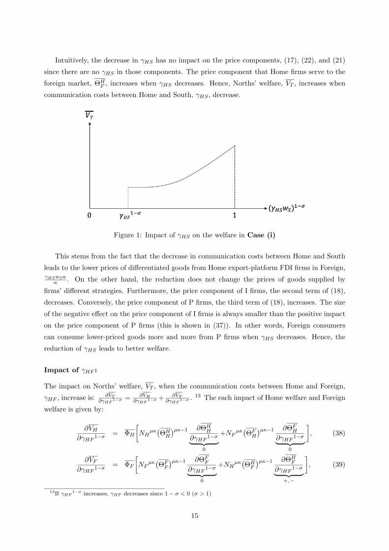
Figure 1: Impact of γHS on the welfare in Case (i)
This stems from the fact that the decrease in communication costs between Home and South
leads to the lower prices of differentiated goods from Home export-platform FDI firms in Foreign,γHSwSa
α . On the other hand, the reduction does not change the prices of goods supplied by
firms’ different strategies. Furthermore, the price component of I firms, the second term of (18),
decreases. Conversely, the price component of P firms, the third term of (18), increases. The size
of the negative effect on the price component of I firms is always smaller than the positive impact
on the price component of P firms (this is shown in (37)). In other words, Foreign consumers
can consume lower-priced goods more and more from P firms when γHS decreases. Hence, the
reduction of γHS leads to better welfare.
Impact of γHF :
The impact on Norths’ welfare, VT , when the communication costs between Home and Foreign,
γHF , increase is: ∂VT∂γHF 1−σ = ∂VH
∂γHF 1−σ + ∂VF∂γHF 1−σ . 13 The each impact of Home welfare and Foreign
welfare is given by:
∂VH∂γHF 1−σ = ΦH
[NH
µκ(ΘHH
)µκ−1 ∂ΘHH
∂γHF 1−σ︸ ︷︷ ︸0
+NFµκ(ΘFH
)µκ−1 ∂ΘFH
∂γHF 1−σ︸ ︷︷ ︸0
], (38)
∂VF∂γHF 1−σ = ΦF
[NF
µκ(ΘFF
)µκ−1 ∂ΘFF
∂γHF 1−σ︸ ︷︷ ︸0
+NHµκ(ΘHF
)µκ−1 ∂ΘHF
∂γHF 1−σ︸ ︷︷ ︸+,−
], (39)
13If γHF1−σ increases, γHF decreases since 1 − σ < 0 (σ > 1)
15

Thus, we get ∂VT∂γHF 1−σ = ∂VF
∂γHF 1−σ . We have a proposition from equations (38) and (39) as follows:
Proposition 2. Norths’ welfare, VT , increases when communication costs between Home and
Foreign, γHF , are larger than γHF∗ while VT decreases when γHF are smaller than γHF
∗ in Case
(i). The term, γHF∗, exists in γHF
∗ ∈ (γHSwS , τ)
Proof.
∂ΘHF
∂γHF 1−σ =
(1−
(k − σ + 1
1− σ
))[fI − fX
γHF 1−σ − τ1−σ
] k−σ+11−σ
...
...−[
fP − fI(γHSwS)1−σ − γHF 1−σ
] k−σ+11−σ
(40)
As I mentioned, 1 − k−σ+11−σ > 0. However, the expression of the second brace can be positive or
negative. If we derive the second order differentiation of (40), the expression becomes:
∂2ΘHF
∂(γHF 1−σ)2=
k − σ + 1
1− σ
(k − σ + 1
1− σ− 1
)[fI − fX
γHF 1−σ − τ1−σ
] k−σ+11−σ 1
γHF 1−σ − τ1−σ ...
...+
[fP − fI
(γHSwS)1−σ − γHF 1−σ
] k−σ+11−σ 1
(γHSwS)1−σ − γHF 1−σ
> 0
The expression of the second brace is positive and the term, k−σ+11−σ
(k−σ+1
1−σ − 1
), is also positive.
Since k−σ+11−σ < 0 and k−σ+1
1−σ − 1 < 0. Therefore, the equation (40) is a convex function. Then, we
put (40) = 0 to get the vertex of this function. The vertex becomes:
(γHF∗)1−σ =
(γHSwS)1−σ +Aτ1−σ
1 +A, (41)
where A = fP−fIfI−fX . Therefore,
∂VT∂γHF 1−σ = ΦFNH
µκ(ΘHF
)µκ−1 ∂ΘHF
∂γHF 1−σ
< 0, if γHF
1−σ < (γHF∗)1−σ,
= 0 if γHF1−σ = (γHF
∗)1−σ,
> 0 if γHF1−σ > (γHF
∗)1−σ.
The relationships of this vertex and γHSwS and τ are as follows:
(γHF∗)1−σ < (γHSwS)1−σ ⇐⇒ τ > γHSwS ,
(γHF∗)1−σ > τ1−σ ⇐⇒ τ > γHSwS .
The above inequalities always hold by the definition. Hence, γHF∗ ∈ (γHSwS , τ) .
The following figure shows the impact of γHF on the welfare:
16
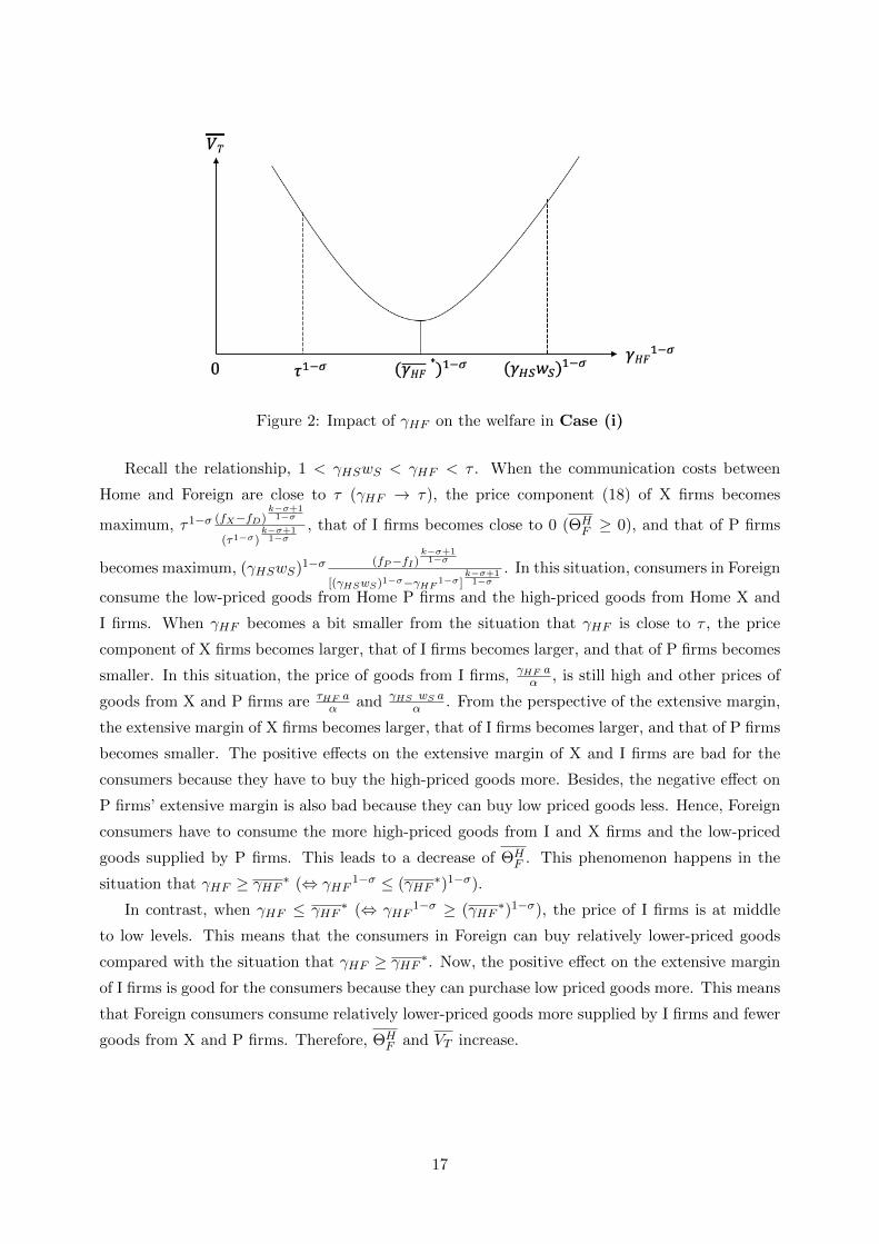
Figure 2: Impact of γHF on the welfare in Case (i)
Recall the relationship, 1 < γHSwS < γHF < τ . When the communication costs between
Home and Foreign are close to τ (γHF → τ), the price component (18) of X firms becomes
maximum, τ1−σ (fX−fD)k−σ+1
1−σ
(τ1−σ)k−σ+1
1−σ, that of I firms becomes close to 0 (ΘH
F ≥ 0), and that of P firms
becomes maximum, (γHSwS)1−σ (fP−fI)k−σ+1
1−σ
[(γHSwS)1−σ−γHF 1−σ ]k−σ+1
1−σ. In this situation, consumers in Foreign
consume the low-priced goods from Home P firms and the high-priced goods from Home X and
I firms. When γHF becomes a bit smaller from the situation that γHF is close to τ , the price
component of X firms becomes larger, that of I firms becomes larger, and that of P firms becomes
smaller. In this situation, the price of goods from I firms, γHF aα , is still high and other prices of
goods from X and P firms are τHF aα and γHS wS a
α . From the perspective of the extensive margin,
the extensive margin of X firms becomes larger, that of I firms becomes larger, and that of P firms
becomes smaller. The positive effects on the extensive margin of X and I firms are bad for the
consumers because they have to buy the high-priced goods more. Besides, the negative effect on
P firms’ extensive margin is also bad because they can buy low priced goods less. Hence, Foreign
consumers have to consume the more high-priced goods from I and X firms and the low-priced
goods supplied by P firms. This leads to a decrease of ΘHF . This phenomenon happens in the
situation that γHF ≥ γHF ∗ (⇔ γHF1−σ ≤ (γHF
∗)1−σ).
In contrast, when γHF ≤ γHF∗ (⇔ γHF
1−σ ≥ (γHF∗)1−σ), the price of I firms is at middle
to low levels. This means that the consumers in Foreign can buy relatively lower-priced goods
compared with the situation that γHF ≥ γHF ∗. Now, the positive effect on the extensive margin
of I firms is good for the consumers because they can purchase low priced goods more. This means
that Foreign consumers consume relatively lower-priced goods more supplied by I firms and fewer
goods from X and P firms. Therefore, ΘHF and VT increase.
17
3.3 Comparison of both welfare effects
Here, I compare the impact of the reduction in communication costs between North and South
on the welfare , ∂VT∂γHS1−σ , with the reduction in communication costs intra Norths on the welfare,
∂VT∂γHF 1−σ , in Case (i). Define ∆ = ∂VT
∂γHS1−σ − ∂VT∂γHF 1−σ . Using (22), (38), and (39), ∆ is explicitly
given by:
∆ = ΦFNHµκ(ΘHF
)µκ−1(
1−(k − σ + 1
1− σ
))...
...
(1 + wS
1−σ)
[fP − fI
(γHSwS)1−σ − γHF 1−σ
] k−σ+11−σ
−[
fI − fXγ1−σHF − τ1−σ
] k−σ+11−σ
. (42)
The above equation can be positive and negative because the impact of the decrease in γHF would
be positive or negative. A point of negation of (42) is as follows:
(1 + wS1−σ)
[fP − fI
(γHSwS)1−σ − γHF 1−σ
] k−σ+11−σ
=
[fI − fX
γHF 1−σ − τ1−σ
] k−σ+11−σ
⇔ (γHF∗∗)1−σ =
(γHFwS)1−σ +Dτ1−σ
1 +D(43)
where D = (1 + wS1−σ)
1−σk−σ+1 fP−fI
fI−fX . At the point, the equation, ∆ = 0, is satisfied. When
∆ > 0, the inequality, γHF1−σ < (γHF
∗∗)1−σ, holds. On the contrary, when ∆ < 0, the inequality
,γHF1−σ > (γHF
∗∗)1−σ, holds. If we differentiate by γHS1−σ, the derivative becomes positive. 14
In other words, at the any values of γHS1−σ, the increase in γHS
1−σ has a larger impact on the
welfare than the impact that γHF1−σ increases. On the other hand, the derivative of γHF
1−σ is
negative. 15 This means that the decrease in γHF makes prices of differentiated goods lower and
then the positive impact on the welfare becomes larger and larger. The following figure shows the
comparison in Case (i):
14 ∂∆∂γHS
1−σ = ΦFNHµκ
(ΘHF
)µκ−1(
1 −(k−σ+1
1−σ
))(1 + wS
1−σ)
[ wS1−σ
(k−σ+1σ−1
)(fP−fI )
k−σ+11−σ
((γHSwS)1−σ−γHF 1−σ)k−σ+11−σ +1
]> 0,
since 1 − k−σ+11−σ > 0 and k−σ+1
σ−1> 0.
15 ∂∆∂γHF
1−σ = ΦFNHµκ
(ΘHF
)µκ−1k−σ+1
1−σ
(1 −
(k−σ+1
1−σ
))(1 + wS
1−σ)
[(fP−fI )
k−σ+11−σ
(γHSwS1−σ−γ1−σ
HF)k−σ+11−σ +1
]< 0
since k−σ+11−σ < 0
18
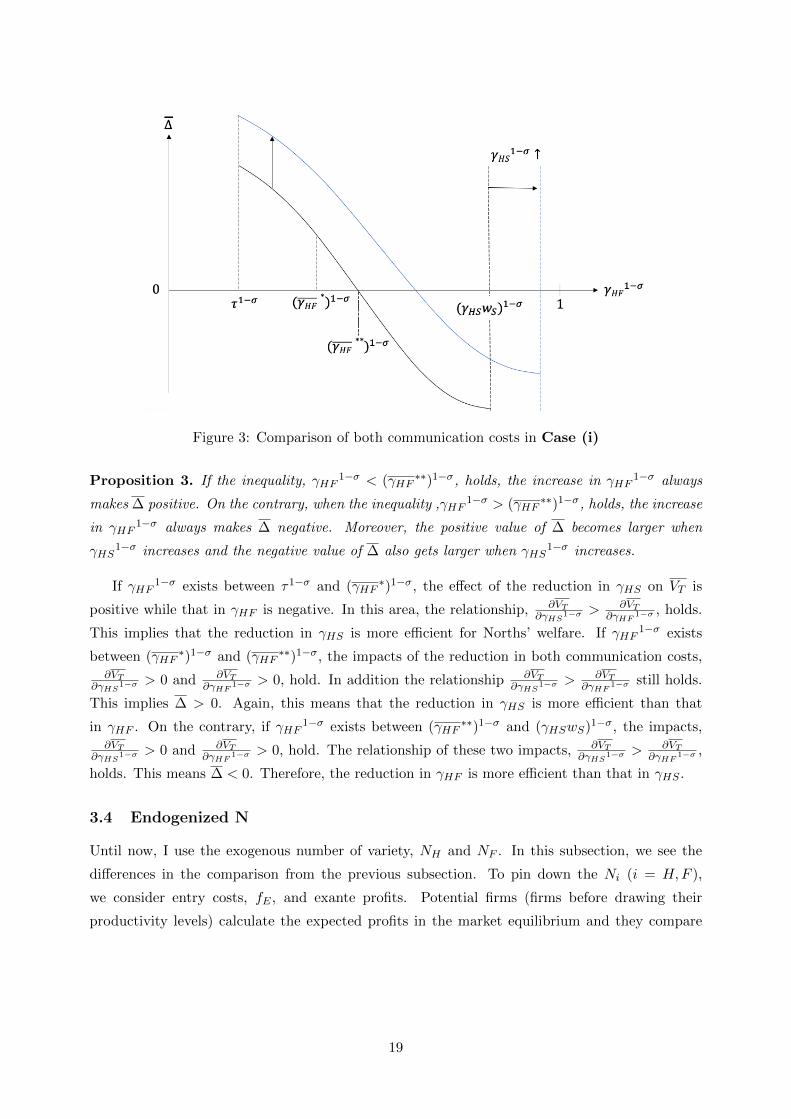
Figure 3: Comparison of both communication costs in Case (i)
Proposition 3. If the inequality, γHF1−σ < (γHF
∗∗)1−σ, holds, the increase in γHF1−σ always
makes ∆ positive. On the contrary, when the inequality ,γHF1−σ > (γHF
∗∗)1−σ, holds, the increase
in γHF1−σ always makes ∆ negative. Moreover, the positive value of ∆ becomes larger when
γHS1−σ increases and the negative value of ∆ also gets larger when γHS
1−σ increases.
If γHF1−σ exists between τ1−σ and (γHF
∗)1−σ, the effect of the reduction in γHS on VT is
positive while that in γHF is negative. In this area, the relationship, ∂VT∂γHS1−σ >
∂VT∂γHF 1−σ , holds.
This implies that the reduction in γHS is more efficient for Norths’ welfare. If γHF1−σ exists
between (γHF∗)1−σ and (γHF
∗∗)1−σ, the impacts of the reduction in both communication costs,∂VT
∂γHS1−σ > 0 and ∂VT∂γHF 1−σ > 0, hold. In addition the relationship ∂VT
∂γHS1−σ >∂VT
∂γHF 1−σ still holds.
This implies ∆ > 0. Again, this means that the reduction in γHS is more efficient than that
in γHF . On the contrary, if γHF1−σ exists between (γHF
∗∗)1−σ and (γHSwS)1−σ, the impacts,∂VT
∂γHS1−σ > 0 and ∂VT∂γHF 1−σ > 0, hold. The relationship of these two impacts, ∂VT
∂γHS1−σ >∂VT
∂γHF 1−σ ,
holds. This means ∆ < 0. Therefore, the reduction in γHF is more efficient than that in γHS .
3.4 Endogenized N
Until now, I use the exogenous number of variety, NH and NF . In this subsection, we see the
differences in the comparison from the previous subsection. To pin down the Ni (i = H,F ),
we consider entry costs, fE , and exante profits. Potential firms (firms before drawing their
productivity levels) calculate the expected profits in the market equilibrium and they compare
19
those profits with the entry costs. Thus, the free entry condition in each country becomes:
fE = (1− α)Bii(
1
α)1−σV i(aD) + (1− α)Bi
j(τ
α)1−σ[V i(aDX)− V i(aXI)]...
...+ (1− α)Bij(γijα
)1−σ[V i(aXI)− V i(aIP )] + (1− α)Bij(γiS wSα
)1−σV i(aIP )...
...− fDGi(aD)− (fXGi(aDX)− fXGi(aXI))− (fHG
i(aXI)− fHGi(aIP ))...
...− fPGi(aIP ), (44)
= χΘii
(Li(X
ii)µ−α1−α
) kσ−1
+ χΘij
(Lj(X
ij)
µ−α1−α
) kσ−1
(i 6= j and i, j = H,F ), (45)
where the right hand side of (44) comes from an integration of prior profits of each countries’ firm
that has not entered the market over the productivity distribution, Gi(a). The expression (45)
comes from the more calculation when I use the productivity cutoffs (9) - (12), the expressions of
the Pareto distribution, G(a) and V (a), and the definitions Bii = Li(X
ii)µ−α1−α and Bi
j = Lj(Xij)
µ−α1−α .
Equation (45) implies that the entry costs are pined down by the weighted exante profits of Home
firms in both markets. Define endogenous varieties as NH and NF in Case (i). Substituting (15)
- (20) into (45), we have the endogenous variety of Home country:
NH =α
kχ
αkk(α−µ)
((ΘHH
)κkLH
κk(1−µ) +(ΘHF
)κkLF
κk(1−µ)
fE
)αk(α−µ)κ
. (46)
For Foreign country’s varieties, we have:
NF =α
kχ
αkk(α−µ)
((ΘFF
)κkLF
κk(1−µ) +(ΘFH
)κkLH
κk(1−µ)
fE
)αk(α−µ)κ
. (47)
Naturally, an increase in entry costs decreases the number of varieties in each country. On the
other hand, an increase in populations, Li and Lj , increases the varieties in each country (the
love of variety effect).
Having NH endogenous, a decrease in communication costs, γHS and γHF , has no effects on
the Norths’ welfare. On the other hand, when NF is endogenous, a reduction in γHS and γHF
has additional effects on the welfare. (see the Appendix for derivatives.)
Lemma 1. ∂NH∂γHS1−σ ,
∂NH∂γHF 1−σ = 0 and ∂NF
∂γHS1−σ > 0 or < 0 and ∂NF∂γHF 1−σ > 0.
The decrease in γHS raises the profits of Foreign entrants, and so the increase in numbers
of the firms of this sector (NF ) has to increase in equilibrium to continue to ensure that firms
earn zero exante profits. On the other hand, the decrease in γHF raises or lower the profits of
Foreign entrants. A vertex of where the positive and negative effects switch is the same condition
as (41). I define the North welfare, VT , when Ni is endogenized as VT Endo in Case (i). This
function’s shape is similar in the case that the number of varieties, Ni, is fixed. More specifically,
VT Endo is increasing in γHS1−σ and VT Endo is a convex function to γHF
1−σ. However, there exist
additional effects of γHS and γHF on welfare. I summarize the results as follows (see Appendix
20
for the proof):
Proposition 4. When Ni (i = H,F ) is endogenized, the impact of the decrease in γHS on Norths’
welfare is always larger than the case of both varieties are fixed. If ∆ is positive, the value of it
becomes larger than that of the case Ni is fixed. On the contrary, if ∆ is negative, the value of it
becomes smaller than that of the case Ni is fixed.
Define ∆Endo = ∂VT Endo∂γHS1−σ − ∂VT Endo
∂γHF 1−σ . The endogenous comparison, ∆Endo, has also the same
negation point, (γHF∗∗)1−σ, as ∆ does. From Proposition 4, when the varieties, Ni, are endog-
enized, the size of positive and negative effects on the welfare becomes larger. This means that
the comparisons of the effects of the reduction in both communication costs also change. More
concretely, the size of the positive value in the endogenous varieties case becomes larger than that
in the exogenous varieties case. At the same time, the size of the negative value in the endoge-
nous varieties case also becomes larger than that in the exogenous varieties case. The following
proposition sums up this change (see Appendix for the details):
Proposition 5. When Ni is endogenous, ∆Endo is 0 if γHF1−σ = (γHF
∗∗)1−σ, positive if
γHF1−σ < (γHF
∗∗)1−σ, and negative if γHF1−σ > (γHF
∗∗)1−σ. In addition, negative and pos-
itive sizes of ∆Endo are always larger than ∆.
4 Welfare analysis: Case (ii)
I explain the welfare analysis in Case (ii) in this section. Case (ii) is the situation that South
is a developing country. Recall the conditions of Case (ii) are fD < fX < fP < fI and
aD1−σ < aDX
1−σ < aXP1−σ < aPI
1−σ. The inequality, aD1−σ < aDX
1−σ < aXP1−σ < aPI
1−σ,
implies γHF1−σ > (γHSwS)1−σ > τ1−σ from (12) and (13). The method of the analysis is the
same as the previous section.
4.1 Welfare
The welfare in each country is defined as (31). Each welfare function is given by:
VH = wH +1− µµ
[(k
α
)χ
]µκ[(NHΘH
H
)µκ+
(NFΘF
H
)µκ]LH
µκ(k−αk−α)α , (48)
VF = wF +1− µµ
[(k
α
)χ
]µκ[(NFΘF
F
)µκ+
(NHΘH
F
)µκ ]LF
µκ(k−αk−α)α . (49)
Then, North’s welfare becomes:
VT = wH + wF +1− µµ
[(k
α
)χ
]µκ[(NHΘH
H
)µκ+
(NFΘF
H
)µκ]LH
µκ(k−αk−α)α ....
....+1− µµ
[(k
α
)χ
]µκ[(NFΘF
F
)µκ+
(NHΘH
F
)µκ ]LF
µκ(k−αk−α)α . (50)
21
4.2 Each welfare effect
Impact of γHS:
The impact of the decreasing γHS on VH and VF are given by:
∂VH
∂γHS1−σ = ΦH
[NH
µκ(ΘHH
)µκ−1 ∂ΘHH
∂γHS1−σ︸ ︷︷ ︸0
+NFµκ(ΘFH
)µκ−1 ∂ΘFH
∂γHS1−σ︸ ︷︷ ︸0
], (51)
∂VF
∂γHS1−σ = ΦF
[NF
µκ(ΘFF
)µκ−1 ∂ΘFF
∂γHS1−σ︸ ︷︷ ︸0
+NHµκ(ΘHF
)µκ−1 ∂ΘHF
∂γHS1−σ︸ ︷︷ ︸+ ,−
], (52)
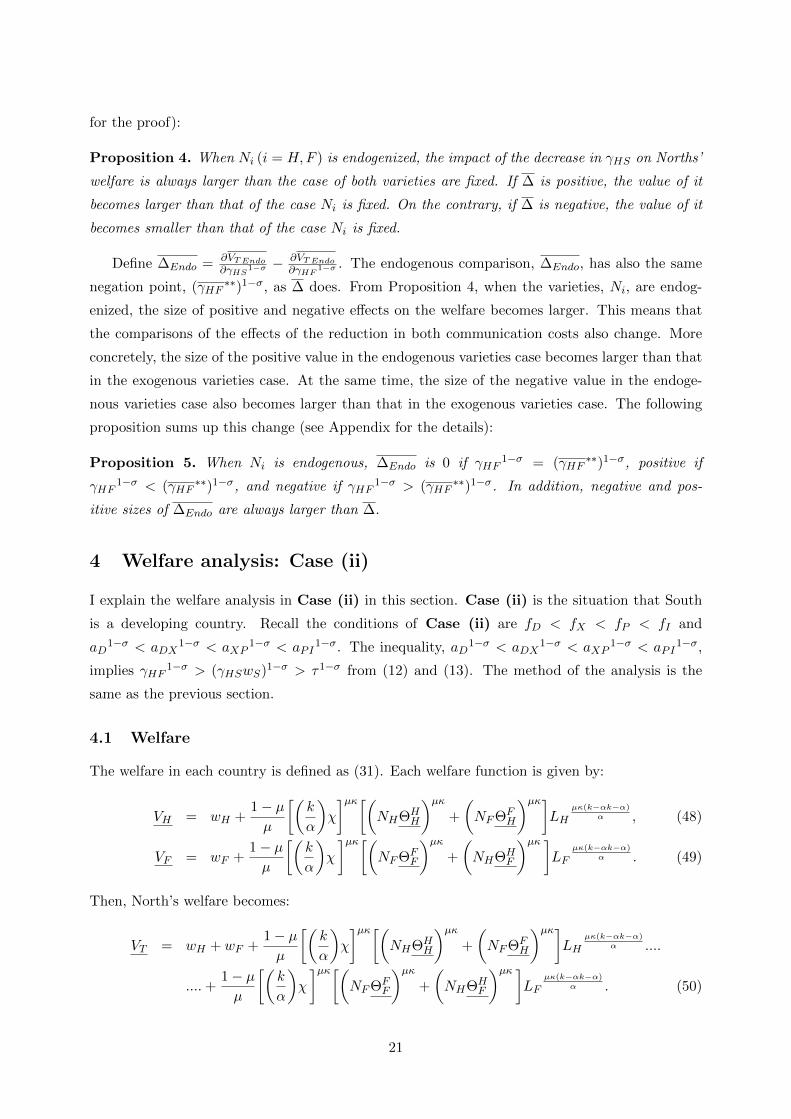
where ΦH and ΦF are in the footnote below. 16 We can draw the following figure from the above
two equations:
Figure 4: Impact of γHS on the welfare
We have the following proposition from the above figure (see Appendix for the proof):
Proposition 6. The Norths’ welfare, VT , increases when communication costs between Home
and South, γHS, are larger than γHS∗ while VT decreases when γHS are smaller than γHS
∗ in
Case (ii). The term, γHS∗, exists in γHSwS
∗ ∈ (γHF , τ). 17
Recall the relationship, 1 < γWE < γHSwS < τ . When the communication costs between
Home and South, γHSwS are closer to τ , the price component of export firms of Home (the first
16
ΦH = κ(1 − µ)
[(k
α
)χ
]µκLH
µκ(k−αk−α)α ,
ΦF = κ(1 − µ)
[(k
α
)χ
]µκLF
µκ(k−αk−α)α .
17To get γHS∗, we put NH
µκ ∂ΘWE
∂γWS1−σ = 0
22
term of (26)) becomes maximum: (fX−fD)k−σ+1
1−σ
[(τ)1−σ ]k−σ+1
1−σ −1, the price component of export-platform FDI
firms of Home (the second term of (26)) becomes close to 0, and the price component of horizontal
FDI firms of Home (the third term of (26)) becomes maximum: (fI−fP )k−σ+1
1−σ
[γHF 1−σ−(γHS wS)1−σ ]k−σ+1
1−σ −1). In
this situation, Foreign consumers consume the low-prices goods from H firms of Home and high-
priced firms from P and X firms of Home. From that situation, if γHS wS decreases a bit, the first
term of (26) increases, the second term of (26) increases, and the third term of (26) decreases.
The price of goods from P firms, γHS wS aα , is still high and the prices from I and X are γHF a
α
and τ aα . For the extensive margins, the extensive margin of X firms becomes more massive, that
of P firms becomes larger, and that of I firms becomes smaller. More concretely, the positive
effect on X and P’s extensive margin is terrible for the consumers because they can purchase the
high-priced goods more. The negative effect on I firms’ extensive margin is also bad because they
can buy low-priced goods less. Therefore, Foreign consumers have to consume high-priced goods
more from P and X firms and low-priced goods less from I firms. This leads to a decrease of ΘHF .
This reduction in ΘHF occurs when (γHSwS)1−σ < (γHS
∗wS)1−σ.
On the contrary, when (γHSwS)1−σ ≥ (γHS∗wS)1−σ holds, the price of p firms is at middle
to low levels. The positive effect on the extensive margin of X and the negative impact on the
extensive margin of I firms are bad for the consumers. In contrast, the positive impact on the
extensive margin of P firms is promising. The latter effect dominates the former effects. Hence,
Foreign consumers can purchase low-priced goods more from P firms. This leads to an increase
of ΘHF and the better welfare VT .
Impact of γHF :
The impact on the world welfare, VT , when the communication costs between Home and Foreign,
γHF , increase is:∂VT
∂γHF 1−σ =∂VH
∂γHF 1−σ +∂VF
∂γHF 1−σ .
∂VH
∂γHF 1−σ = ΦH
[NH
µκ∂ΘH
H
∂γHF 1−σ︸ ︷︷ ︸0
+NFµκ
∂ΘFH
∂γHF 1−σ︸ ︷︷ ︸0
], (53)
∂VF
∂γHF 1−σ = ΦF
[NF
µκ∂ΘF
F
∂γHF 1−σ︸ ︷︷ ︸0
+NHµκ
∂ΘHF
∂γHF 1−σ︸ ︷︷ ︸+
], (54)
The following figure shows the impact on the welfare:
23
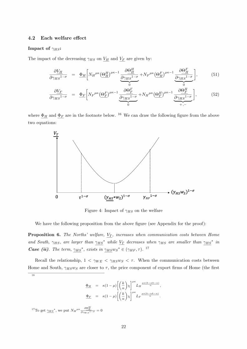
Figure 5: Impact of γHF on the welfare
Intuitively, the decrease in γHF has no impact on the partial ex-ante profits,(25), (30), and
(29) since there is no term, γHF , in those price components. For the impact on ΘHF , it increases
when γHF decreases (see Appendix for the proof). Therefore, the Norths’ welfare, VT , increases
when communication costs between Home and Foreign, γHF decrease. This result comes from
the fact that the decrease in communication costs leads to an increase in the lower prices of
differentiated goods from Home horizontal FDI firms that is available in Foreign. Hence, VT ,
increases. We have a proposition from equations (53) and (54) as follows:
Proposition 7. The Norths’ welfare, VT , increases when communication costs between Home
and Foreign, γHF , decreases in Case (ii).
4.3 Comparison of both welfare effects
Define ∆ =∂VT
∂γHS1−σ −∂VT
∂γHF 1−σ in Case (ii). Using (30), (53), and (54), we can rewrite ∆ as:
∆ = ΦFNHµκ(ΘHF
)µκ−1(
1−(k − σ + 1
1− σ
))wS
1−σ[
fP − fX(γHSwS)1−σ − τ1−σ
] k−σ+11−σ
...
...− (1 + wS1−σ)
[fI − fP
γHF 1−σ − (γHSwS)1−σ
] k−σ+11−σ
. (55)
The above equation can be positive and negative because the impact of the decrease in γHS would
be positive or negative. A point of negation of (55) are as follow:
(1 + wS1−σ)
[fI − fP
γHF 1−σ − (γHSwS)1−σ
] k−σ+11−σ
= wS1−σ[
fP − fX(γHSwS)1−σ − τ1−σ
] k−σ+11−σ
⇔ (γHS∗∗wS)1−σ =
γHF1−σ +Dτ1−σ
1 +D(56)
where D =(
1+wS1−σ
wS1−σ
) 1−σk−σ+1 fI−fP
fP−fX . At the negating point, the equation, ∆ = 0, is satisfied. When
∆ > 0, the inequality, γHS1−σ > (γHS
∗∗)1−σ, holds and when ∆ < 0, the inequality, γHS1−σ <
24
(γHS∗∗)1−σ, holds. If we differentiate ∆ by γHS
1−σ, the derivative becomes positive.18 On the
other hand, the derivative of γHS1−σ is negative.19 The following figure shows the comparison in
Case (ii):
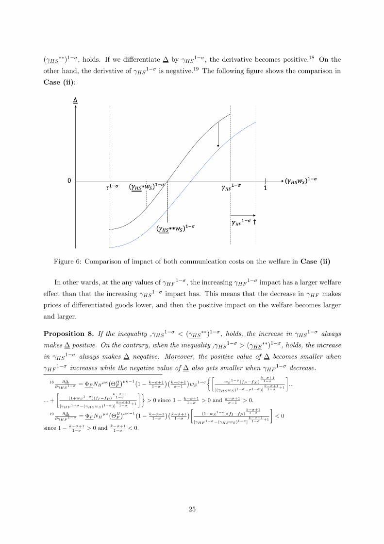
Figure 6: Comparison of impact of both communication costs on the welfare in Case (ii)
In other wards, at the any values of γHF1−σ, the increasing γHF
1−σ impact has a larger welfare
effect than that the increasing γHS1−σ impact has. This means that the decrease in γHF makes
prices of differentiated goods lower, and then the positive impact on the welfare becomes larger
and larger.
Proposition 8. If the inequality ,γHS1−σ < (γHS
∗∗)1−σ, holds, the increase in γHS1−σ always
makes ∆ positive. On the contrary, when the inequality ,γHS1−σ > (γHS
∗∗)1−σ, holds, the increase
in γHS1−σ always makes ∆ negative. Moreover, the positive value of ∆ becomes smaller when
γHF1−σ increases while the negative value of ∆ also gets smaller when γHF
1−σ decrease.
18 ∂∆
∂γHS1−σ = ΦFNH
µκ(ΘHF
)µκ−1(1 − k−σ+1
1−σ
)(k−σ+1σ−1
)wS
1−σ[
wS1−σ(fP−fX )
k−σ+11−σ
[(γHSwS)1−σ−τ1−σ)]k−σ+11−σ +1
]...
...+
[(1+wS
1−σ)(fI−fP )k−σ+11−σ
[γHF1−σ−(γHSwS)1−σ)]
k−σ+11−σ +1
]> 0 since 1 − k−σ+1
1−σ > 0 and k−σ+1σ−1
> 0.
19 ∂∆
∂γHF1−σ = ΦFNH
µκ(ΘHF
)µκ−1(1 − k−σ+1
1−σ
)(k−σ+1
1−σ
)[ (1+wS1−σ)(fI−fP )
k−σ+11−σ
[γHF1−σ−(γHSwS)1−σ ]
k−σ+11−σ +1
]< 0
since 1 − k−σ+11−σ > 0 and k−σ+1
1−σ < 0.
25
4.4 Endogenized N
To pin down the Ni (i = H,F ) in Case (ii), the procedure is same as Case (i) (we put entry
costs equalize to exante profits). Then, the free entry condition in each country becomes:
fE = (1− α)Bii(
1
α)1−σV i(aD) + (1− α)Bi
j(τ
α)1−σ[V i(aDX)− V i(aXP )]...
...+ (1− α)Bij(γiS wSα
)1−σ[V i(aXP )− V i(aPI)] + (1− α)Bij(γijα
)1−σV i(aPI)...
...− fDGi(aD)− (fXGi(aDX)− fXGi(aXP ))− (fHG
i(aXP )− fHGi(aPI))...
...− fPGi(aPI), (57)
= χΘii
(Li(X
ii)µ−α1−α
) kσ−1
+ χΘij
(Lj(X
ij)
µ−α1−α
) kσ−1
(i 6= j and i, j = H,F ). (58)
The right hand side of (57) is the integration of the prior profits of each potential firm over the
productivity distribution, Gi(a). Using productivity cutoffs (9) - (14), the expressions of the
Pareto distribution, Gi(a) and V i(a), and the definitions Bii = Li(X
ii)µ−α1−α and Bi
j = Lj(Xij)
µ−α1−α ,
we have (58). Equation (58) implies that the entry costs are equalize to the weighted exante profits
of Home firms in both markets. Define the endogenous Ni as Ni in Case (ii). Substituting (23)
- (28) into (58), we have the endogenous variety of Home country:
NH =α
kχ
αkk(α−µ)
((ΘHH
)κkLH
κk(1−µ) +(ΘHF
)κkLF
κk(1−µ)
fE
)αk(α−µ)κ
. (59)
For Foreign country’s varieties, we have:
NF =α
kχ
αkk(α−µ)
((ΘFF
)κkLF
κk(1−µ) +(ΘFH
)κkLH
κk(1−µ)
fE
)αk(α−µ)κ
. (60)
Same as in Case (i), an increase in fE decreases the number of varieties in each country but an
increase in populations in each country, Li and Lj , increase the varieties in each country (the love
of variety effect holds).
When NH is endogenous, a decrease in γHS and γHF has no effects on world welfare. On the
other hand, when NF is endogenous, γHS and γHF , has additional effects on Norths’ welfare. (see
the Appendix for derivatives.)
Lemma 2.∂NH
∂γHS1−σ ,∂NH
∂γHF 1−σ = 0 and∂NF
∂γHS1−σ > 0 and∂NF
∂γHF 1−σ > 0 or < 0.
The decrease in γHS raises the profits of Foreign entrants, and so the increase in numbers of
the firms of this sector (NF ) has to increase in equilibrium. On the other hand, the decrease in
γHS raises or lowers the profits of Foreign entrants. A vertex where the positive and negative
effects switch is γHS1−σ = (γHS
∗∗)1−σ. Define the North welfare, VT , when Ni is endogenized as
VT Endo in Case (ii). This function has a similar shape in the case that the number of varieties,
26
Ni, is fixed. The impact of the reduction in each communication cost on VT Endo becomes:
∂VT Endo
∂γHS1−σ = ΦH
(NHΘH
H
)µκ−1ΘHH
∂NH
∂γHS1−σ + ΦF
(NHΘH
F
)µκ−1ΘHF
∂NH
∂γHS1−σ +∂VT
∂γHS1−σ , (61)
∂VT Endo
∂γHF 1−σ = ΦH
(NHΘH
H
)µκ−1ΘHH
∂NH
∂γHF 1−σ + ΦF
(NHΘH
F
)µκ−1ΘHF
∂NH
∂γHF 1−σ +∂VT
∂γHF 1−σ . (62)
More concretely, VT Endo is a convex function to γHS1−σ and VT Endo is increasing in γHF
1−σ.
However, there exist additional effects of γHS and γHF on welfare. Thus, the shape of the
functions,∂VT
∂γHS1−σ and∂VT
∂γHF 1−σ , is same as the case that the number of varieties, Ni, is fixed. To
sum up the result, we have the following proposition (see Appendix for the proof):
Proposition 9. When Ni (i = H,F ) is endogenized, the impact of the increase in γHS1−σ on the
welfare is always larger than the case that both varieties are fixed. If ∆ is positive, the value of it
becomes more extensive than that of the case Ni is fixed. On the contrary, if ∆ is negative, the
value of it becomes smaller than that of the case Ni is fixed.
Define ∆Endo =∂VT Endo∂γHS1−σ −
∂VT Endo∂γHF 1−σ . The endogenous comparison, ∆Endo, has also the same
negation point, (γHS∗∗)1−σ, as ∆ does. From Proposition 9, when Ni is endogenized, the size of
positive and negative effects on the welfare becomes larger. Concretely, the size of the positive
value in the endogenous varieties case becomes larger than that in the exogenous varieties case.
Simultaneously, the size of the endogenous varieties case’s negative value also becomes more
extensive than that in the exogenous varieties case. The following proposition sums up the this
change (see Appendix for the details):
Proposition 10. When Ni is endogenous, ∆Endo is 0 if γHS1−σ = (γHS
∗∗)1−σ, negative if
γHS1−σ < (γHS
∗∗)1−σ, and positive if γHS1−σ > (γHS
∗∗)1−σ. In addition, negative and positive
sizes of ∆Endo are always larger than ∆.
5 Conclusion
This paper has shown how the reduction in communication costs between North and South and
between both Norths affected the North country’s welfare. I use a three-country model with
heterogeneous firms and communication costs between an HQ and a plant to analyze these effects.
Focusing on the equilibrium where four firm’s strategies: domestic, export, horizontal FDI, and
export-platform FDI co-exist, I consider two equilibrium, Case (i) and Case (ii). In both cases,
the second highest productive firms’ reduction in communication costs would harm the Norths’
welfare. Concretely, when communication costs between Home and Foreign in Case (i) and Home
and South in Case (i) are high and when they decrease a bit, the consumers in Foreign have to
buy high priced goods more. Then, these worsen the Norths’ welfare. These results imply that
firms have to consider which communication cost should be decreased carefully. This is because
if firms are not familiar with the market structure, they may harm other countries’ welfare.
27
Furthermore, I have compared the effects of reducing both the communication costs of Home
and Foreign and Home and South in each case. In Case (i), the reduction in communication
costs between Home and South / Home and Foreign leads to larger welfare improvement when
the costs between Home and Foreign are high/low. In Case (i), the reduction in communication
costs between Home and South / Home and Foreign leads the larger welfare improvement when
the costs between Home and South are low/high.
My analysis focuses on only communication costs between an HQ and a plant. However, one
may think the firms also incur communication costs between the HQ and the customer. These
costs are also crucial determinants of firms’ HQs and plants location because firms’ communication
with customers is necessary feedback for producing varieties. In future work, I hope to consider
the model with these different communication costs.
References
[1] Battiston, D., J. Blanes I Vidal and T. Kirchmaier (2017), “Is distance dead? Face-to-face
communication and productivity in teams”, CEPR Discussion Paper, No.11924.
[2] Charnoz, P., C. Lelarge and C. Trevien (2018), “Communication costs and the internal orga-
nization of multi-plant businesses: Evidence from the impact of the French high-speed rail,”
CEPR Discussion Paper, No.12585.
[3] Chor, D. (2009), “Subsidies for FDI: Implication from a model with heterogeneous firms,”
Journal of International Economics, 78, 113–125.
[4] Cristea, A.D. (2015), “The effect of communication costs on trade in headquarter service,”
Review of World Economics, 151, 225–289.
[5] Dischinger, M., Knoll, B. and Riedel, N. (2014), “There’s no place like home: The prof-
itability gap between headquarters and their foreign subsidiaries,” Journal of Economics and
Management Strategy, 23, 369–95.
[6] Ekholm, K., Forslid, R. and Markusen, J.R. (2007), “Export-platform foreign direct invest-
ment,” Journal of the European Economic Association, 5, 776–795.
[7] Feinberg, S.E. and Keane, M.P. (2006), “Accounting for the Growth of MNC-Based Trade
Using a Structural Model of U.S. MNCs,” American Economic Review, 96, 1515–1558.
[8] Giroud, X. (2013), “Proximity and investment: Evidence from plant-level data,” The
Quarterly Journal of Economics, 128, 861–915.
[9] Gokan, T., Kicho, S. and Thisse, J.F. (2018), “How do trade and communication costs shape
the spatial organization of firms ?,” Journal of Urban Economics, 113, 103191.
28
[10] Grossman, G.M., Helpman, E. and Szeidl, A. (2006), “Optimal integration strategies for the
multinational firm,” Journal of International Economics, 70, 216–238.
[11] Hanson, G, Mataloni, R, and Slaughter, M. (2005), “Vertical Production Networks in Multi-
national Firms,” Review of Economics and Statistics, 87, 664—678.
[12] Helpman, E. (2006), “Trade, FDI, and the organization of firms,” Journal of Economic
Literature, XLIV, 589–630.
[13] Helpman, E., Melitz, M.J. and Yeaple, S.R. (2004), “Export versus FDI with heterogeneous
firms,” American Economic Review, 94, 300–316.
[14] Hollander, S. and A. Verriest (2016), “Bridging the gap: The design of bank loan contracts
and distance,” Journal of F inancial Economics, 119, 399 – 419.
[15] Ito, T. (2013), ”Export-Platform Foreign Direct Investment: Theory and Evidence”, The
World Economy, 36, 563 – 581.
[16] Kalnins, A. and F. Lafontaine (2013), “Too far away? The effect of distance to headquarters
on business estab- lishment performance”, American Economic Journal : Microeconomics,
5, 157 – 179.
[17] Kok, R. and Acikgoz, E, B. (2002) “Analyses of FDI determinants in developing countries,”
International Journal of Social Economics, 36, 105–123.
[18] Markusen, J. (2002), Multinational F irms and the Theory of International Trade,
Boston, MIT Press.
[19] Melitz, M.J. (2003), “The impact of trade on intra-industry reallocations and aggregate
industry productivity,” Econometrica, 71, 1695–1725.
[20] Ministry of Economy, Trade and Industry, (2010)-(2020), Survey on Overseas Business
Activities,
[21] Montout, S. and Zitouna, H. (2005), “Does North-South Integration affect Multinational
Firms’ Strategies?,” Review of International Economics, 13, 485–500.
[22] Mrazova, M. and Neary, P. (2012), “Firm Selection into Export-Platform Foreign Direct
Investment”, Working Paper.
[23] Neary, P. (2002) “Foreign Direct Investment and the Single Market,” The Manchester
School, 70, 291–314.
[24] Oldenski, L. (2012), “Export versus FDI and the communication of complex information,”
Journal of International Economics, 87, 312–322.
29
[25] Rydzek, B., Egger, P. and Riezman, R. (2015) “The effects of cultural distance on multi-unit
firms”, ECONSTOR working paper.
[26] Tintelnot, F. (2017), “Global production with export platforms,” The Quarterly Journal
of Economics, 132, 157–209.
Appendix
Section 3 : Case (i)
Derivations for Lemma 1
∂NH∂γHS1−σ = α
kχαk
k(α−µ)
((ΘHH
)κkLH
κk(1−µ)+(
ΘHF
)κkLF
κk(1−µ)
fE
) ακk(α−µ)
−1
...
...
(κk(
ΘHH
)κk−1 ∂ΘHH
∂γHS1−σ︸ ︷︷ ︸0
LHκk(1−µ)+κk
(ΘHF
)κk−1 ∂ΘHF
∂γHS1−σ︸ ︷︷ ︸+
LFκk(1−µ)
fE
)= +
∂NH∂γHF 1−σ = α
kχαk
k(α−µ)
((ΘHH
)κkLH
κk(1−µ)+(
ΘHF
)κkLF
κk(1−µ)
fE
) ακk(α−µ)
−1
...
...
(κk(
ΘHH
)κk−1 ∂ΘHH
∂γHF 1−σ︸ ︷︷ ︸0
LHκk(1−µ)+κk
(ΘHF
)κk−1 ∂ΘHF
∂γHF 1−σ︸ ︷︷ ︸+ ,−
LFκk(1−µ)
fE
)= ±
∂NF∂γHS1−σ = α
kχαk
k(α−µ)
((ΘFF
)κkLF
κk(1−µ)+(
ΘFH
)κkLH
κk(1−µ)
fE
) ακk(α−µ)
−1
...
...
(κk(
ΘFF
)κk−1 ∂ΘFF
∂γHS1−σ︸ ︷︷ ︸0
LFκk(1−µ)+κk
(ΘFH
)κk−1 ∂ΘFH
∂γHS1−σ︸ ︷︷ ︸0
LHκk(1−µ)
fE
)= 0
∂NF∂γHF 1−σ = α
kχαk
k(α−µ)
((ΘFF
)κkLF
κk(1−µ)+(
ΘFH
)κkLH
κk(1−µ)
fE
) ακk(α−µ)
−1
...
...
(κk(
ΘFF
)κk−1 ∂ΘFF
∂γHF 1−σ︸ ︷︷ ︸0
LFκk(1−µ)+κk
(ΘFH
)κk−1 ∂ΘFH
∂γHF 1−σ︸ ︷︷ ︸0
LHκk(1−µ)
fE
)= 0
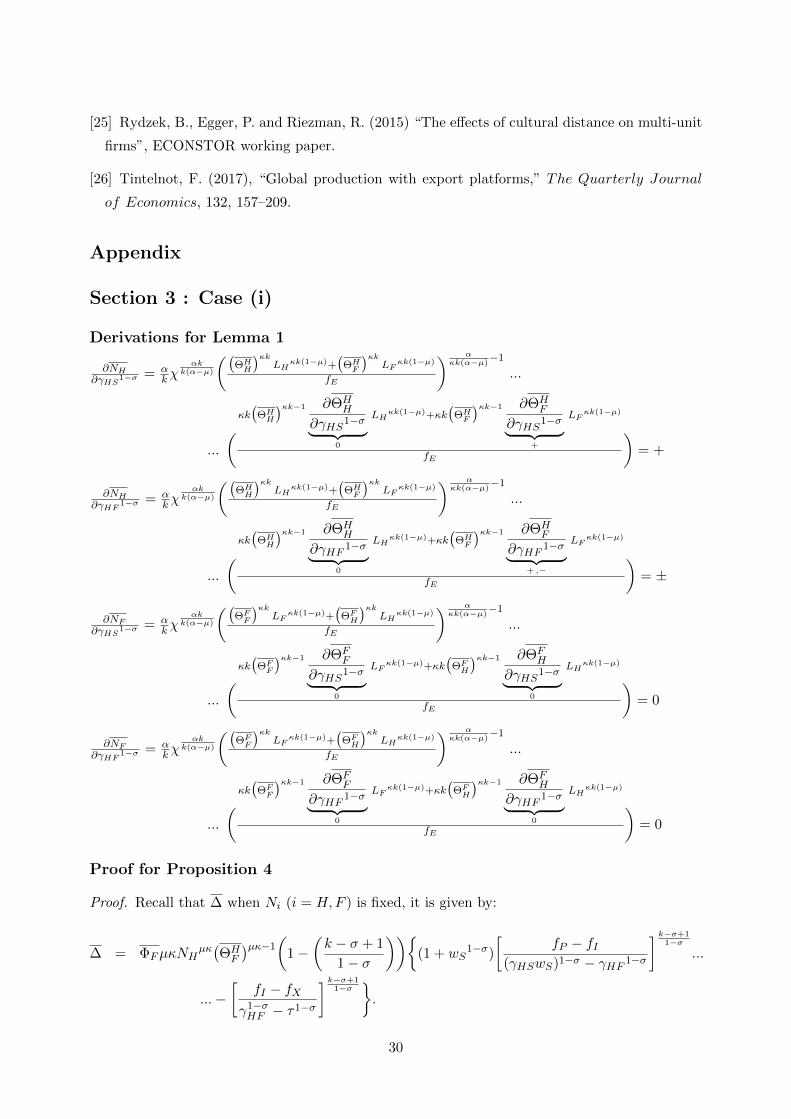
Proof for Proposition 4
Proof. Recall that ∆ when Ni (i = H,F ) is fixed, it is given by:
∆ = ΦFµκNHµκ(ΘHF
)µκ−1(
1−(k − σ + 1
1− σ
))(1 + wS
1−σ)
[fP − fI
(γHSwS)1−σ − γHF 1−σ
] k−σ+11−σ
...
...−[
fI − fXγ1−σHF − τ1−σ
] k−σ+11−σ
.
30
Define that ∆ when Ni (i = H,F ) is endogenous as ∆Endo = ∂VT Endo∂γHS1−σ − ∂VT Endo
∂γHF 1−σ .
The term, ∂VT Endo∂γHS1−σ , can be rewritten as:
∂VT Endo∂γHS1−σ = ΦH
(NHΘH
H
)µκ−1ΘHH
∂NH
∂γHS1−σ + ΦF
(NHΘH
F
)µκ−1ΘHF
∂NH
∂γHS1−σ +∂VT
∂γHS1−σ . (A.1)
From Derivations for Lemma 1, the term, ∂NH∂γHS1−σ , is given by:
∂NH
∂γHS1−σ = Υ
(∂ΘH
F
∂γHS1−σ
), (A.2)
where Υ = αkχ
αkk(α−µ)
((ΘHH
)κkLH
κk(1−µ)+(
ΘHF
)κkLF
κk(1−µ)
fE
) ακk(α−µ)
−1(κk(
ΘHF
)κk−1LF
κk(1−µ)
fE
).
Recall that∂ΘHF
∂γHS1−σ is always positive. Hence, ∂VT Endo∂γHS1−σ has additional positive effects when Ni is
endogenous compared with ∂VT∂γHS1−σ . The following figure shows this fact:
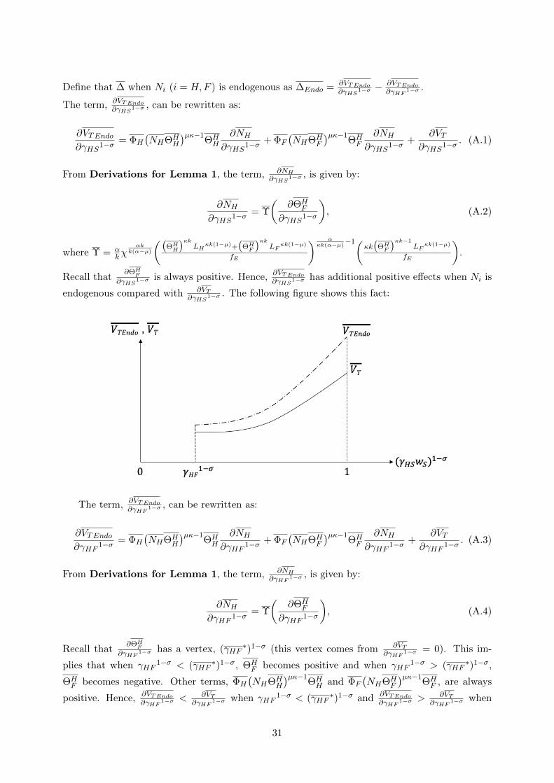
The term, ∂VT Endo∂γHF 1−σ , can be rewritten as:
∂VT Endo∂γHF 1−σ = ΦH
(NHΘH
H
)µκ−1ΘHH
∂NH
∂γHF 1−σ + ΦF
(NHΘH
F
)µκ−1ΘHF
∂NH
∂γHF 1−σ +∂VT
∂γHF 1−σ . (A.3)
From Derivations for Lemma 1, the term, ∂NH∂γHF 1−σ , is given by:
∂NH
∂γHF 1−σ = Υ
(∂ΘH
F
∂γHF 1−σ
), (A.4)
Recall that∂ΘHF
∂γHF 1−σ has a vertex, (γHF∗)1−σ (this vertex comes from ∂VT
∂γHF 1−σ = 0). This im-
plies that when γHF1−σ < (γHF
∗)1−σ, ΘHF becomes positive and when γHF
1−σ > (γHF∗)1−σ,
ΘHF becomes negative. Other terms, ΦH
(NHΘH
H
)µκ−1ΘHH and ΦF
(NHΘH
F
)µκ−1ΘHF , are always
positive. Hence, ∂VT Endo∂γHF 1−σ < ∂VT
∂γHF 1−σ when γHF1−σ < (γHF
∗)1−σ and ∂VT Endo∂γHF 1−σ > ∂VT
∂γHF 1−σ when
31
γHF1−σ > (γHF
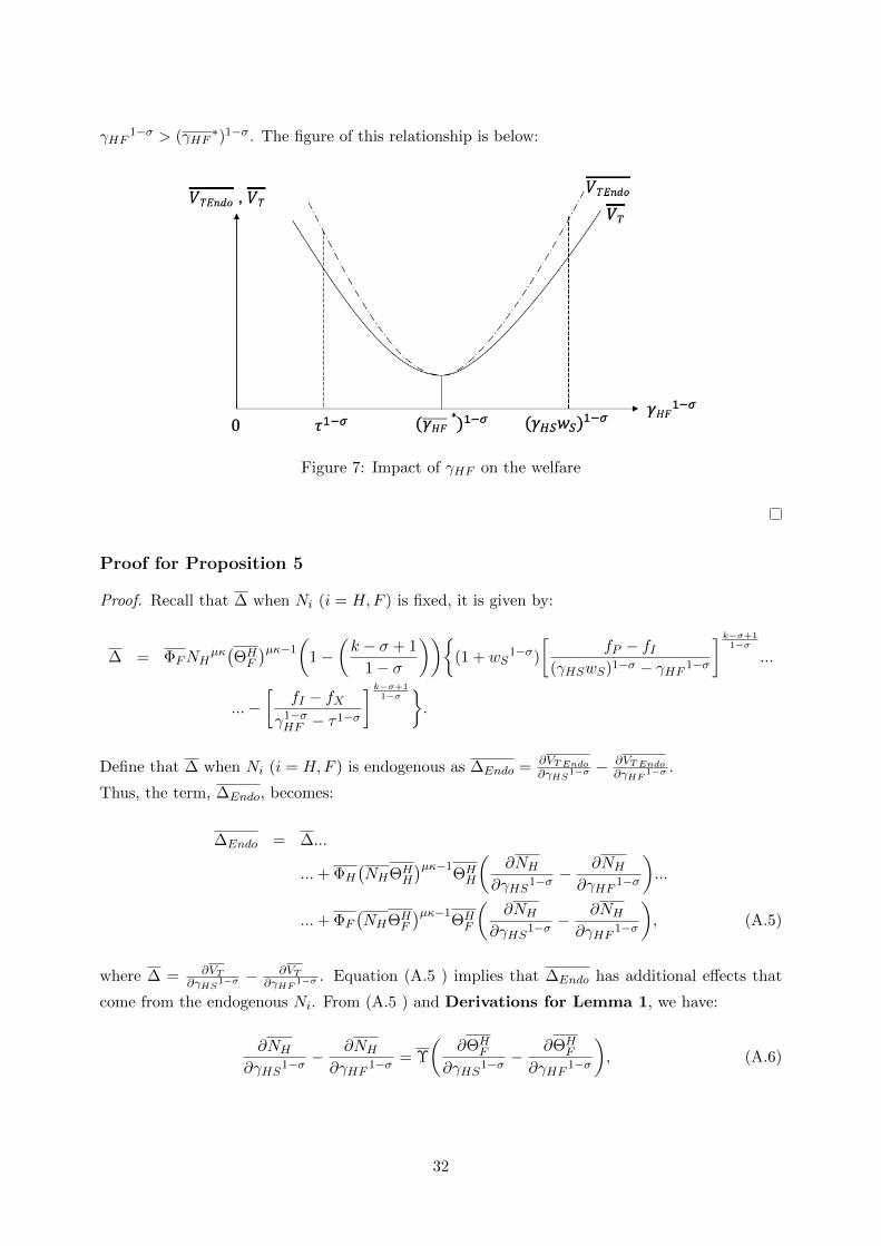
∗)1−σ. The figure of this relationship is below:
Figure 7: Impact of γHF on the welfare
Proof for Proposition 5
Proof. Recall that ∆ when Ni (i = H,F ) is fixed, it is given by:
∆ = ΦFNHµκ(ΘHF
)µκ−1(
1−(k − σ + 1
1− σ
))(1 + wS
1−σ)
[fP − fI
(γHSwS)1−σ − γHF 1−σ
] k−σ+11−σ
...
...−[
fI − fXγ1−σHF − τ1−σ
] k−σ+11−σ
.
Define that ∆ when Ni (i = H,F ) is endogenous as ∆Endo = ∂VT Endo∂γHS1−σ − ∂VT Endo
∂γHF 1−σ .
Thus, the term, ∆Endo, becomes:
∆Endo = ∆...
...+ ΦH
(NHΘH
H
)µκ−1ΘHH
(∂NH
∂γHS1−σ −∂NH
∂γHF 1−σ
)...
...+ ΦF
(NHΘH
F
)µκ−1ΘHF
(∂NH
∂γHS1−σ −∂NH
∂γHF 1−σ
), (A.5)
where ∆ = ∂VT∂γHS1−σ − ∂VT
∂γHF 1−σ . Equation (A.5 ) implies that ∆Endo has additional effects that
come from the endogenous Ni. From (A.5 ) and Derivations for Lemma 1, we have:
∂NH
∂γHS1−σ −∂NH
∂γHF 1−σ = Υ
(∂ΘH
F
∂γHS1−σ −∂ΘH
F
∂γHF 1−σ
), (A.6)
32
where Υ = αkχ
αkk(α−µ)
((ΘHH
)κkLH
κk(1−µ)+(
ΘHF
)κkLF
κk(1−µ)
fE
) ακk(α−µ)
−1(κk(
ΘHF
)κk−1LF
κk(1−µ)
fE
).
The right hand side of (A.6 ) is:
Υ
(∂ΘH
F
∂γHS1−σ −∂ΘH
F
∂γHF 1−σ
)= Υ
(1−
(k − σ + 1
1− σ
))(1 + wS
1−σ)
[fP − fI
(γHSwS)1−σ − γHF 1−σ
] k−σ+11−σ
...
...−[
fI − fXγHF 1−σ − τ1−σ
] k−σ+11−σ
. (A.7)
This equation can be positive or negative. A point of negation of this equation is equal to
(γHF∗∗)1−σ. At this point, Υ
(∂ΘHF
∂γHS1−σ −∂ΘHF
∂γHF 1−σ
)= 0 holds. If γHF
1−σ < (γHF∗∗)1−σ holds,
Υ
(∂ΘHF
∂γHS1−σ −∂ΘHF
∂γHF 1−σ
)> 0 holds and if γHF
1−σ > (γHF∗∗)1−σ holds, Υ
(∂ΘHF
∂γHS1−σ −∂ΘHF
∂γHF 1−σ
)> 0
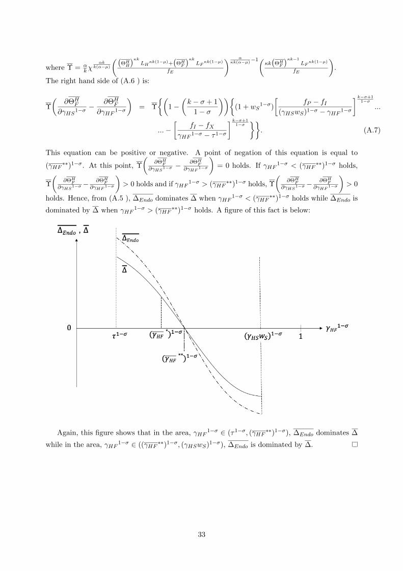
holds. Hence, from (A.5 ), ∆Endo dominates ∆ when γHF1−σ < (γHF
∗∗)1−σ holds while ∆Endo is
dominated by ∆ when γHF1−σ > (γHF
∗∗)1−σ holds. A figure of this fact is below:
Again, this figure shows that in the area, γHF1−σ ∈ (τ1−σ, (γHF
∗∗)1−σ), ∆Endo dominates ∆
while in the area, γHF1−σ ∈ ((γHF
∗∗)1−σ, (γHSwS)1−σ), ∆Endo is dominated by ∆.
33
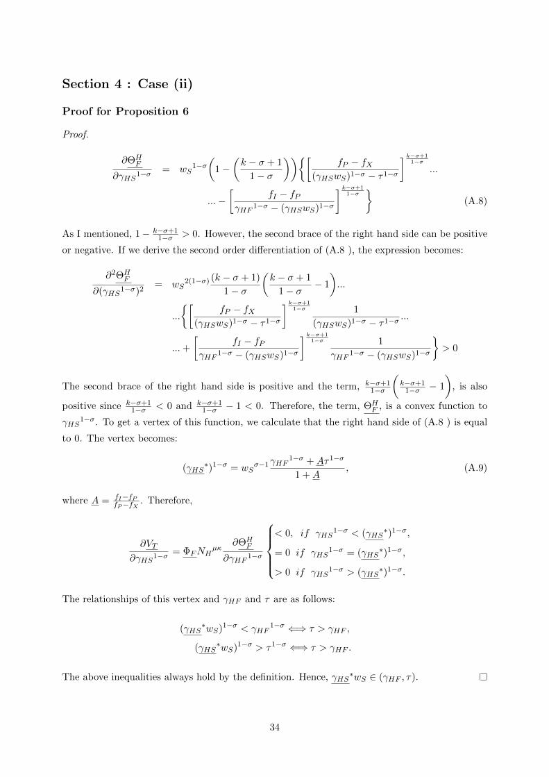
Section 4 : Case (ii)
Proof for Proposition 6
Proof.
∂ΘHF
∂γHS1−σ = wS1−σ(
1−(k − σ + 1
1− σ
))[fP − fX
(γHSwS)1−σ − τ1−σ
] k−σ+11−σ
...
...−[
fI − fPγHF 1−σ − (γHSwS)1−σ
] k−σ+11−σ
(A.8)
As I mentioned, 1− k−σ+11−σ > 0. However, the second brace of the right hand side can be positive
or negative. If we derive the second order differentiation of (A.8 ), the expression becomes:
∂2ΘHF
∂(γHS1−σ)2= wS
2(1−σ) (k − σ + 1)
1− σ
(k − σ + 1
1− σ− 1
)...
...
[fP − fX
(γHSwS)1−σ − τ1−σ
] k−σ+11−σ 1
(γHSwS)1−σ − τ1−σ ...
...+
[fI − fP
γHF 1−σ − (γHSwS)1−σ
] k−σ+11−σ 1
γHF 1−σ − (γHSwS)1−σ
> 0
The second brace of the right hand side is positive and the term, k−σ+11−σ
(k−σ+1
1−σ − 1
), is also
positive since k−σ+11−σ < 0 and k−σ+1
1−σ − 1 < 0. Therefore, the term, ΘHF , is a convex function to
γHS1−σ. To get a vertex of this function, we calculate that the right hand side of (A.8 ) is equal
to 0. The vertex becomes:
(γHS∗)1−σ = wS
σ−1γHF1−σ +Aτ1−σ
1 +A, (A.9)
where A = fI−fPfP−fX . Therefore,
∂VT
∂γHS1−σ = ΦFNHµκ
∂ΘHF
∂γHF 1−σ
< 0, if γHS
1−σ < (γHS∗)1−σ,
= 0 if γHS1−σ = (γHS
∗)1−σ,
> 0 if γHS1−σ > (γHS
∗)1−σ.
The relationships of this vertex and γHF and τ are as follows:
(γHS∗wS)1−σ < γHF
1−σ ⇐⇒ τ > γHF ,
(γHS∗wS)1−σ > τ1−σ ⇐⇒ τ > γHF .
The above inequalities always hold by the definition. Hence, γHS∗wS ∈ (γHF , τ).
34
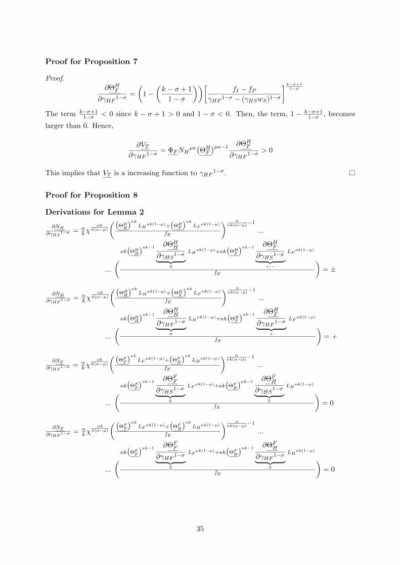
Proof for Proposition 7
Proof.∂ΘH
F
∂γHF 1−σ =
(1−
(k − σ + 1
1− σ
))[fI − fP
γHF 1−σ − (γHSwS)1−σ
] k−σ+11−σ
The term k−σ+11−σ < 0 since k − σ + 1 > 0 and 1 − σ < 0. Then, the term, 1 − k−σ+1
1−σ , becomes
larger than 0. Hence,
∂VT
∂γHF 1−σ = ΦFNHµκ(ΘHF
)µκ−1 ∂ΘHF
∂γHF 1−σ > 0
This implies that VT is a increasing function to γHF1−σ.
Proof for Proposition 8
Derivations for Lemma 2
∂NH∂γHS1−σ = α
kχαk
k(α−µ)
((ΘHH
)κkLH
κk(1−µ)+(
ΘHF
)κkLF
κk(1−µ)
fE
) ακk(α−µ)
−1
...
...
(κk(
ΘHH
)κk−1 ∂ΘHH
∂γHS1−σ︸ ︷︷ ︸0
LHκk(1−µ)+κk
(ΘHF
)κk−1 ∂ΘHF
∂γHS1−σ︸ ︷︷ ︸+,−
LFκk(1−µ)
fE
)= ±
∂NH∂γHF 1−σ = α
kχαk
k(α−µ)
((ΘHH
)κkLH
κk(1−µ)+(
ΘHF
)κkLF
κk(1−µ)
fE
) ακk(α−µ)
−1
...
...
(κk(
ΘHH
)κk−1 ∂ΘHH
∂γHF 1−σ︸ ︷︷ ︸0
LHκk(1−µ)+κk
(ΘHF
)κk−1 ∂ΘHF
∂γHF 1−σ︸ ︷︷ ︸+
LFκk(1−µ)
fE
)= +
∂NF∂γHS1−σ = α
kχαk
k(α−µ)
((ΘFF
)κkLF
κk(1−µ)+(
ΘFH
)κkLH
κk(1−µ)
fE
) ακk(α−µ)
−1
...
...
(κk(
ΘFF
)κk−1 ∂ΘFF
∂γHS1−σ︸ ︷︷ ︸0
LFκk(1−µ)+κk
(ΘFH
)κk−1 ∂ΘFH
∂γHS1−σ︸ ︷︷ ︸0
LHκk(1−µ)
fE
)= 0
∂NF∂γHF 1−σ = α
kχαk
k(α−µ)
((ΘFF
)κkLF
κk(1−µ)+(
ΘFH
)κkLH
κk(1−µ)
fE
) ακk(α−µ)
−1
...
...
(κk(
ΘFF
)κk−1 ∂ΘFF
∂γHF 1−σ︸ ︷︷ ︸0
LFκk(1−µ)+κk
(ΘFH
)κk−1 ∂ΘFH
∂γHF 1−σ︸ ︷︷ ︸0
LHκk(1−µ)
fE
)= 0
35

Proof for Proposition 9
Proof. Impact of γHF on the welfare of endogenous Ni :
Recall the term, ∂VT Endo∂γHS1−σ , can be rewritten as:
∂VT Endo
∂γHS1−σ = ΦH
(NHΘH
H
)µκ−1ΘHH
∂NH
∂γHS1−σ + ΦF
(NHΘH
F
)µκ−1ΘHF
∂NH
∂γHS1−σ +∂VT
∂γHS1−σ . (A.10)
From Derivations for Lemma 2, the term,∂NH
∂γHS1−σ , is given by:
∂NH
∂γHS1−σ = Υ
(∂ΘH
F
∂γHS1−σ
), (A.11)
where Υ = αkχ
αkk(α−µ)
((ΘHH
)κkLH
κk(1−µ)+(
ΘHF
)κkLF
κk(1−µ)
fE
) ακk(α−µ)
−1(κk(
ΘHF
)κk−1LF
κk(1−µ)
fE
).
Recall that∂ΘHF
∂γHS1−σ has a vertex, γHS∗. Then,
∂ΘHF∂γHS1−σ < 0 if (γHSwS)1−σ < (γHS
∗wS)1−σ and∂ΘHF
∂γHS1−σ > 0 if (γHSwS)1−σ > (γHS∗wS)1−σ. This implies that
∂NH∂γHS1−σ < 0 when (γHSwS)1−σ <
(γHS∗wS)1−σ and
∂NH∂γHS1−σ > 0 when (γHSwS)1−σ > (γHS
∗wS)1−σ because Υ is positive. In
other words,∂VT Endo∂γHS1−σ has additional negative effects when (γHSwS)1−σ < (γHS
∗wS)1−σ and has
additional positive effects when (γHSwS)1−σ > (γHS∗wS)1−σ. Hence, from (A.10 ) ,the slope of
∂VT Endo∂γHS1−σ is larger than that of
∂VT∂γHS1−σ . The following figure shows this fact:
Figure 8: Endogenous Ni: Impact of γHS on the welfare in Case (ii)
[Impact of γHS on the welfare of endogenous Ni ]
The term, ∂VT Endo∂γHF 1−σ , can be rewritten as:
∂VT Endo
∂γHF 1−σ = ΦH
(NHΘH
H
)µκ−1ΘHH
∂NH
∂γHF 1−σ + ΦF
(NHΘH
F
)µκ−1ΘHF
∂NH
∂γHF 1−σ +∂VT
∂γHF 1−σ .(A.12)
36
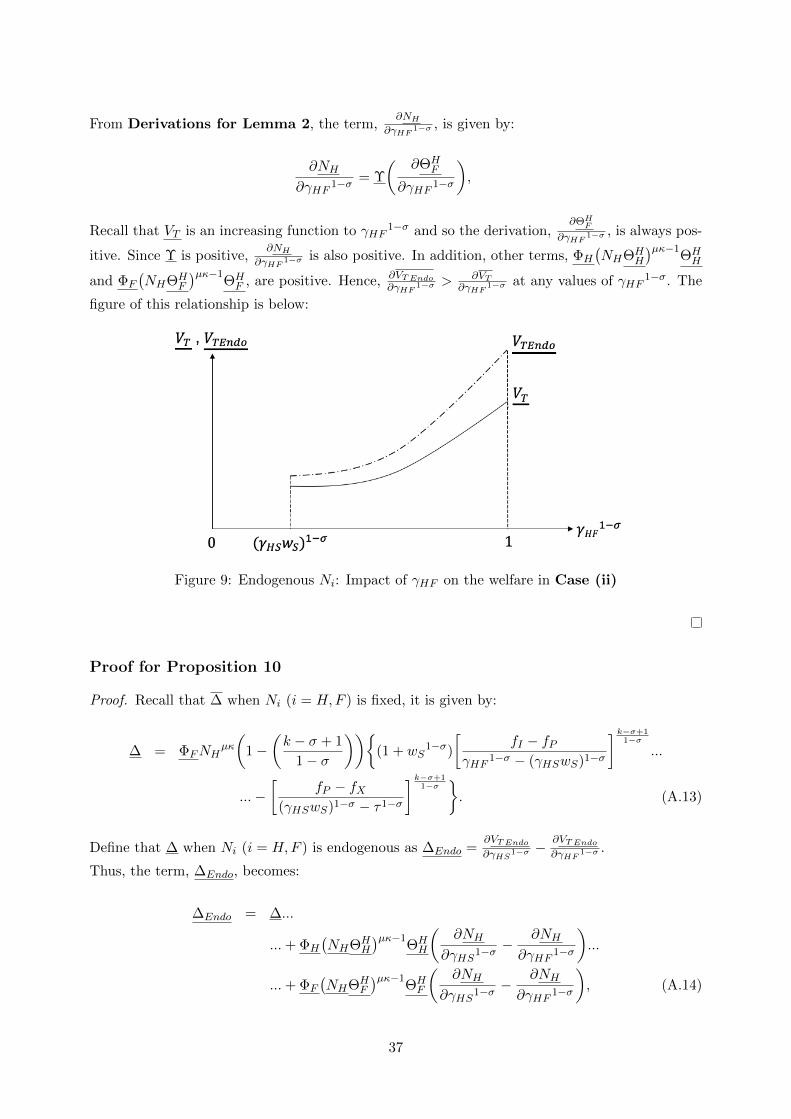
From Derivations for Lemma 2, the term,∂NH
∂γHF 1−σ , is given by:
∂NH
∂γHF 1−σ = Υ
(∂ΘH
F
∂γHF 1−σ
),
Recall that VT is an increasing function to γHF1−σ and so the derivation,
∂ΘHF∂γHF 1−σ , is always pos-
itive. Since Υ is positive,∂NH
∂γHF 1−σ is also positive. In addition, other terms, ΦH
(NHΘH
H
)µκ−1ΘHH
and ΦF
(NHΘH
F
)µκ−1ΘHF , are positive. Hence, ∂VT Endo
∂γHF 1−σ >∂VT
∂γHF 1−σ at any values of γHF1−σ. The
figure of this relationship is below:
Figure 9: Endogenous Ni: Impact of γHF on the welfare in Case (ii)
Proof for Proposition 10
Proof. Recall that ∆ when Ni (i = H,F ) is fixed, it is given by:
∆ = ΦFNHµκ
(1−
(k − σ + 1
1− σ
))(1 + wS
1−σ)
[fI − fP
γHF 1−σ − (γHSwS)1−σ
] k−σ+11−σ
...
...−[
fP − fX(γHSwS)1−σ − τ1−σ
] k−σ+11−σ
. (A.13)
Define that ∆ when Ni (i = H,F ) is endogenous as ∆Endo =∂VT Endo∂γHS1−σ −
∂VT Endo∂γHF 1−σ .
Thus, the term, ∆Endo, becomes:
∆Endo = ∆...
...+ ΦH
(NHΘH
H
)µκ−1ΘHH
(∂NH
∂γHS1−σ −∂NH
∂γHF 1−σ
)...
...+ ΦF
(NHΘH
F
)µκ−1ΘHF
(∂NH
∂γHS1−σ −∂NH
∂γHF 1−σ
), (A.14)
37
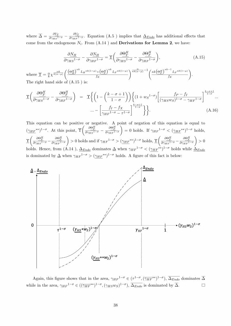
where ∆ =∂VT
∂γHS1−σ −∂VT
∂γHF 1−σ . Equation (A.5 ) implies that ∆Endo has additional effects that
come from the endogenous Ni. From (A.14 ) and Derivations for Lemma 2, we have:
∂NH
∂γHS1−σ −∂NH
∂γHF 1−σ = Υ
(∂ΘH
F
∂γHS1−σ −∂ΘH
F
∂γHF 1−σ
), (A.15)
where Υ = αkχ
αkk(α−µ)
((ΘHH
)κkLH
κk(1−µ)+(
ΘHF
)κkLF
κk(1−µ)
fE
) ακk(α−µ)
−1(κk(
ΘHF
)κk−1LF
κk(1−µ)
fE
).
The right hand side of (A.15 ) is:
Υ
(∂ΘH
F
∂γHS1−σ −∂ΘH
F
∂γHF 1−σ
)= Υ
(1−
(k − σ + 1
1− σ
))(1 + wS
1−σ)
[fP − fI
(γHSwS)1−σ − γHF 1−σ
] k−σ+11−σ
...
...−[
fI − fXγHF 1−σ − τ1−σ
] k−σ+11−σ
. (A.16)
This equation can be positive or negative. A point of negation of this equation is equal to
(γHF∗∗)1−σ. At this point, Υ
(∂ΘHF
∂γHS1−σ −∂ΘHF
∂γHF 1−σ
)= 0 holds. If γHF
1−σ < (γHF∗∗)1−σ holds,
Υ
(∂ΘHF
∂γHS1−σ −∂ΘHF
∂γHF 1−σ
)> 0 holds and if γHF
1−σ > (γHF∗∗)1−σ holds, Υ
(∂ΘHF
∂γHS1−σ −∂ΘHF
∂γHF 1−σ
)> 0
holds. Hence, from (A.14 ), ∆Endo dominates ∆ when γHF1−σ < (γHF
∗∗)1−σ holds while ∆Endo
is dominated by ∆ when γHF1−σ > (γHF
∗∗)1−σ holds. A figure of this fact is below:
Again, this figure shows that in the area, γHF1−σ ∈ (τ1−σ, (γHF
∗∗)1−σ), ∆Endo dominates ∆
while in the area, γHF1−σ ∈ ((γHF
∗∗)1−σ, (γHSwS)1−σ), ∆Endo is dominated by ∆.
38