Heterogeneity and the FDI versus Export Decision

of Japanese Manufacturers∗

Keith Head† John Ries‡

October 28, 2003

We investigate whether productivity differences explain why some manufacturers

sell only to the domestic market while others serve foreign markets through exports

and/or FDI. When overseas production offers no cost advantages, our model predicts

that investors should be more productive than exporters. An extension allowing for

low-cost foreign production can reverse this prediction. Data for 1070 large Japanese

firms reveal that firms that invest abroad and export are more productive than firms

that just export. Among overseas investors, more productive firms span a wider range

of host-country income levels.

JEL classification: F120, F230Keywords: FDI, exports, productivity, heterogeneous firms

∗We thank Kyoji Fukao, Jota Ishikawa, an anonymous referee, and participants at the 15th AnnualTRIO Conference held in Tokyo, December 10–11, 2002 for their helpful comments.

†Sauder School of Business, University of British Columbia, 2053 Main Mall, Vancouver, BC, V6T1Z2,Canada. Tel: (604)822-8492, Fax: (604)822-8477, Email:keith.head@ubc.ca

‡Sauder School of Business, University of British Columbia, 2053 Main Mall, Vancouver, BC, V6T1Z2,Canada. Tel: (604)822-8493 Email:john.ries@ubc.ca

1 Introduction

Theoretical and empirical research has revealed the factors that underlie the decision of

firms to serve foreign consumers through foreign direct investment (FDI) or exporting.

Evidence shows that firms prefer FDI to exporting when trade costs are high and plant-

level scale economies are low. In any given industry, however, we observe that some

firms engage in FDI, some export, and some do neither. There is limited understanding

of heterogeneous actions of firms facing the same trade and investment opportunities.

This paper builds on research of Helpman, Melitz, and Yeaple (forthcoming), here-

after HMY, examining the role of differences in the productivity levels of firms in an

industry as explanations for the presence of purely domestic firms, exporting firms, and

investing firms. We develop an alternative model that yields the predictions found by

HMY and then test these predictions. We also extend the model and show that the order-

ing predicted by HMY can be reversed if the foreign country is the low-cost production

site. We categorize 1070 publicly traded Japanese firms in 1989 into groups according to

whether they export and have foreign direct investment. Then we use various measures

of the productivity of these firms to investigate productivity differences across these

groups.

Our analysis contributes to the literature investigating the export versus FDI decision

of firms. Brainard (1997) shows how trade costs, market size, and plant-level economies

of scale interact to explain the export and FDI decision of firms producing differentiated

products. She shows that the share of firms that export in an industry is an increasing

function of scale economies and a decreasing function of trade costs and foreign market

size. Using U.S. exports and foreign affiliate sales data for 63 industries in 27 countries,

1

Brainard finds that export shares decrease with trade and freight costs and increase with

plant-level scale economies.

Brainard identifies a possible equilibrium where some firms export and others do

foreign investment. Her theory, however, simply specifies the share of firms doing each

activity and does not predict which firms do which activity. HMY extend this line of

research by identifying a role for productivity differences to explain the choice. HMY

develop a free entry model where firms have heterogeneous productivity levels and

each produce a differentiated product. Consumers have CES preferences and goods are

subject to “iceberg” transportation costs. They find that the least productive firms do

not serve the foreign market, the most productive firms engage in FDI, and the mid-

range firms export. Their paper extends Melitz (forthcoming) that shows that only the

most productive firms in an industry export. Bernard, Eaton, Jenson, and Kortum (2003)

use a Ricardian model of trade in differentiated products and demonstrate that the most

productive firms in an industry export. Neither of the latter papers consider the option

to reach foreign consumers through direct investment.

Bernard and Jenson (1999) measure the total factor productivity (TFP) of U.S. man-

ufacturing plants over the period 1984–1992. They find that exporting plants exhibit

higher TFP than non-exporters (after controlling for industry and state fixed effects)

and productive plants are most likely to become exporters. Bernard and Jenson also

investigate whether exporting “causes” greater TFP by examining productivity growth

of exporters and non-exporters. Their results showing that exporters have significantly

slower TFP growth than non-exporters do not support the proposition that exporting

generates TFP growth. HMY analyze the relationship between the export to FDI ratio

2

of 4-digit U.S. manufacturing industries and the dispersion of sales levels in these indus-

tries and find support for their model. Girma and Kneller (2003) test the predictions

of HMY using data on 5,332 firms in the United Kingdom. Based on tests of stochastic

dominance, they find support for the proposition that the productivity distribution of

multinationals dominates that of export firms which dominates that of non-exporters.

We extend both the theoretical and empirical literature. The next section develops a

simple linear demand model that generates the HMY predictions under the assumption

that factors prices are equal and that firms serve foreign consumers either by exporting

or opening up a new manufacturing facility in the foreign country. Section 3 explains

how we classify the 1070 Japanese manufacturing firms into four groups and identifies

the different ways we measure productivity. It goes on to examine differences in produc-

tivity across the groups of firms to test the predictions of our model in the case of equal

wages. Section 4 considers international factor price differences and the possibility that

firms may choose to close down the home plant when they invest abroad. We find that

low productivity firms are the ones most attracted to the option of relocating to a low-

cost foreign country. Data on host-country incomes reveal that low productivity firms

invest primarily in low-income countries. The final section summarizes our findings.

2 Theoretical Predictions of the Basic Model

We provide a simple theoretical model that generates predictions that can be tested with

our data. It replicate’s HMY’s predictions on the ordering of productivity across firms

that sell only to the domestic market and those that serve foreign markets through ex-

3

ports and/or FDI. Our analysis, therefore, reveals that their theoretical results do not

rely upon their assumptions of CES preferences and iceberg transportation costs.

We evaluate firm i producing a differentiated product that is deciding whether to

serve a foreign market f and, if so, whether to export or invest abroad (FDI). A third

way to serve the foreign market would be to license the production process or brand to

a foreign firm. Firm-level data on licensing by Japanese firms are not available. Aggre-

gate Japanese data suggest that exporting and direct investment are the primary modes

through which Japanese firms serve foreign markets: For 2001, the Bank of Japan re-

ports exports of 46.6 trillion yen, a stock of direct investment abroad of 39.6 trillion yen,

and total royalties and license fees of just 1.3 trillion yen. For these reasons, we do not

consider the possibility of licensing in the ensuing analysis.

We assume that marginal costs are constant and equal to w/Ai where w represents

wages in the country where the goods are produced and Ai is a measure of productivity

that is specific to firm i and varies across firms. The firm evaluates the profits of export-

ing and foreign investment and chooses the mode that generates the highest profits.

We assume the following quadratic utility function for consumers:

U = Q0 +N∑

i=1

[Qi − (1/2)Q2i ].

Products i = 1...N are each manufactured by a single firm whereas Q0 is a competi-

tively supplied numeraire good. Utility maximization yields a linear demand for firm

i’s product: Pi = 1−Qi, for i ≥ 1. Thus, this set-up allows us to model each firm’s deci-

sion as if it were a monopolist facing a linear demand curve. We therefore omit the firm

4

subscripts in the rest of the derivation. Obviously these assumptions are not designed

for realism but rather to examine the FDI versus export decision in a truly “minimal”

model of the market.

Exports incur a per unit trade cost of τ whereas FDI allows the firm to avoid trade

costs but requires a fixed cost K to operate the facility. As this model is static, K com-

prises reoccurring expenses that do not vary with output as well as sunk costs incurred

when the plant is opened.

If a firm chooses to neither export nor do FDI it earns zero profits in the foreign

market. We assume equal wages of w in the home and foreign country, an assumption

that yields the same result as HMY regarding the ordering of productivity across types

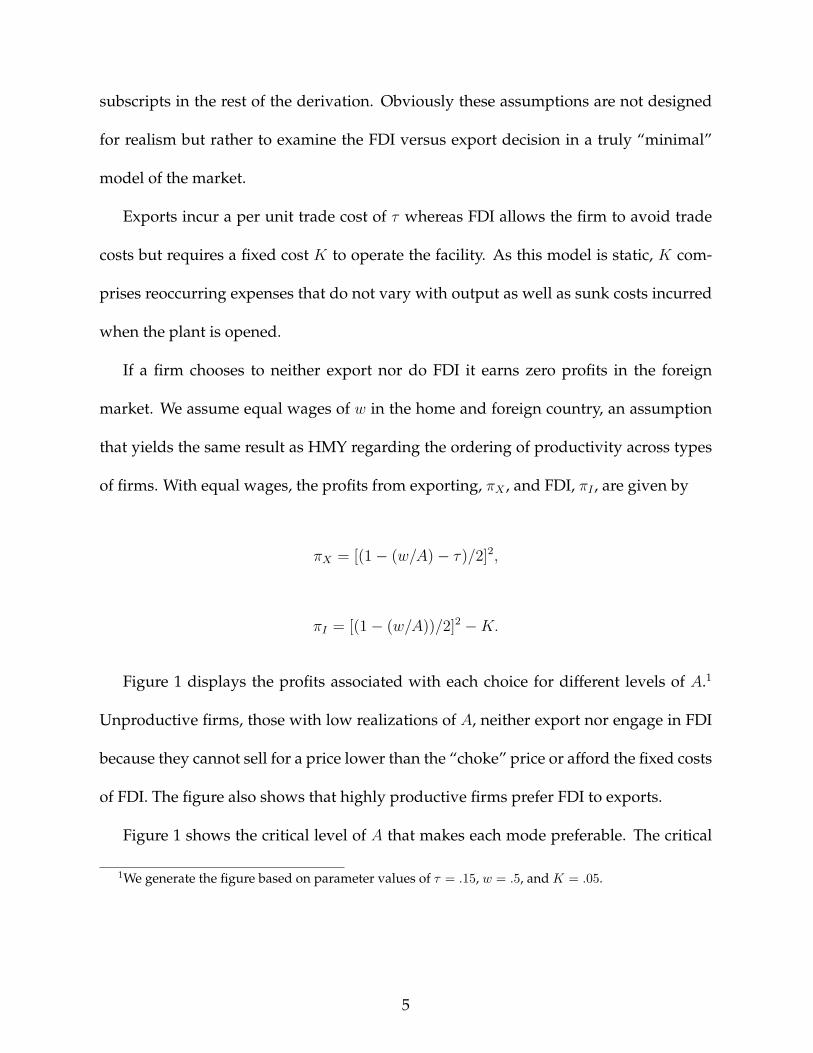
of firms. With equal wages, the profits from exporting, πX , and FDI, πI , are given by

πX = [(1− (w/A)− τ)/2]2,

πI = [(1− (w/A))/2]2 −K.

Figure 1 displays the profits associated with each choice for different levels of A.1

Unproductive firms, those with low realizations of A, neither export nor engage in FDI

because they cannot sell for a price lower than the “choke” price or afford the fixed costs

of FDI. The figure also shows that highly productive firms prefer FDI to exports.

Figure 1 shows the critical level of A that makes each mode preferable. The critical

1We generate the figure based on parameter values of τ = .15, w = .5, and K = .05.

5

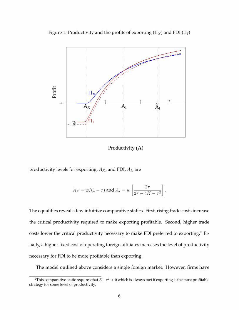
Figure 1: Productivity and the profits of exporting (ΠX) and FDI (ΠI)

Productivity (A)

Pro

fit0

AX AI A~I

x

ΠX

y

ΠI

z

− K− 1.15K

productivity levels for exporting, AX , and FDI, AI , are

AX = w/(1− τ) and AI = w

[2τ

2τ − 4K − τ 2

].

The equalities reveal a few intuitive comparative statics. First, rising trade costs increase

the critical productivity required to make exporting profitable. Second, higher trade

costs lower the critical productivity necessary to make FDI preferred to exporting.2 Fi-

nally, a higher fixed cost of operating foreign affiliates increases the level of productivity

necessary for FDI to be more profitable than exporting.

The model outlined above considers a single foreign market. However, firms have

2This comparative static requires that K−τ2 > 0 which is always met if exporting is the most profitablestrategy for some level of productivity.

6

the opportunity to sell to consumers in different foreign countries. Our data set does not

contain information on the destination of each firm’s exports. Thus, we are interested

in aggregate exports and FDI. Fixed costs of investment vary across destination coun-

tries for a number of reasons. Countries with high crime rates and political rebellions

increase security costs. Markets where corruption is rife might also require bribes. Fixed

costs could reflect expatriate staffing necessary to implement modern management tech-

niques. In distant and unfamiliar markets, substantial costs might also be required to

gather intelligence and identify optimal production sites.

The dashed line in Figure 1 shows the profits associated with FDI when fixed costs

are increased and portrays how a higher critical level of productivity, denoted AI , is nec-

essary to make FDI preferable. Consider firms with productivity levels corresponding to

points x, y, and z. Firm x exports to both markets, Firm y exports to the high fixed-cost

country and invests in the other country, and Firm z invests in both foreign countries.

Aggregating across markets will yield many firms that do both FDI and exporting.

Our simple model generates the same testable prediction that HMY generate in their

model. Namely, firms that serve only the domestic market, firms that export, firms that

export and do FDI, and firms that serve foreign consumers only through FDI are ordered

according to their productivity levels.

3 Testing the Model Predictions

The first subsection describes the data and the proxies we use for firm productivity. The

second subsection tests the predictions of the basic model.

7

3.1 Data and productivity measures

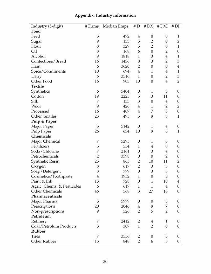
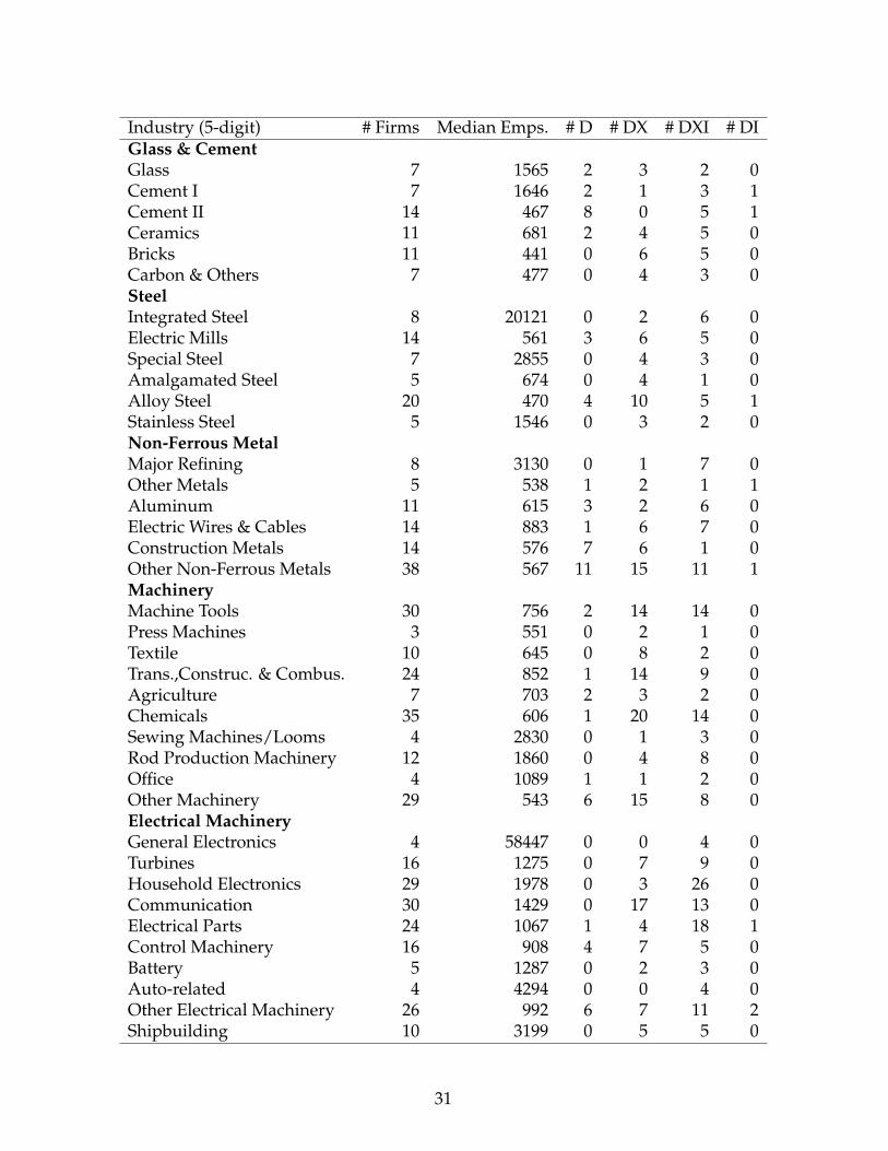
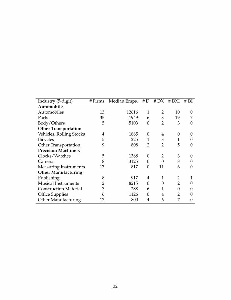
We employ data for 1070 publicly listed Japanese manufacturing firms. Exports, sales,

finished goods purchases, material purchases, depreciable assets, and labour costs are

available from the financial statements of publicly traded companies in Japan. The firms

are classified into 17 2-digit industries and 88 5-digit industries (the appendix contains

a list of these industries). Toyo Keizai (1992) compiles information on the overseas af-

filiates of Japanese companies based on a survey conducted in 1991. They list the host

country, number of employees, date of establishment, equity share, and type of invest-

ment (greenfield or acquisition).

We classify these firms into four groups based on 1989 characteristics. We use D to

represent firms that only serve the domestic market. DX also firms export, DXI firms

export and invest abroad, and DI firms have FDI but do not export. Table 1 provides

information on these groups. The largest group is DXI with 459 firms accounting for

80% of the domestic employment of the 1070 firms. The next largest group is the firms

that export but do not do FDI. There are more firms that sell only to the domestic market

than those that sell to the domestic market and have overseas affiliates but the latter

group comprises larger firms. The table reveals that D firms are the smallest in terms

of average sales, average value added, and average employment whereas DXI firms are

the largest. DX and DI firms lie in between in terms of size with DI being somewhat

larger of the two.

Our theory predicts that there will be an ordering of our four groups according to

productivity. Namely, D firms should be the least productive, followed by DX firms,

then DXI firms, with DI firms being the most productive. To test this prediction, we

8

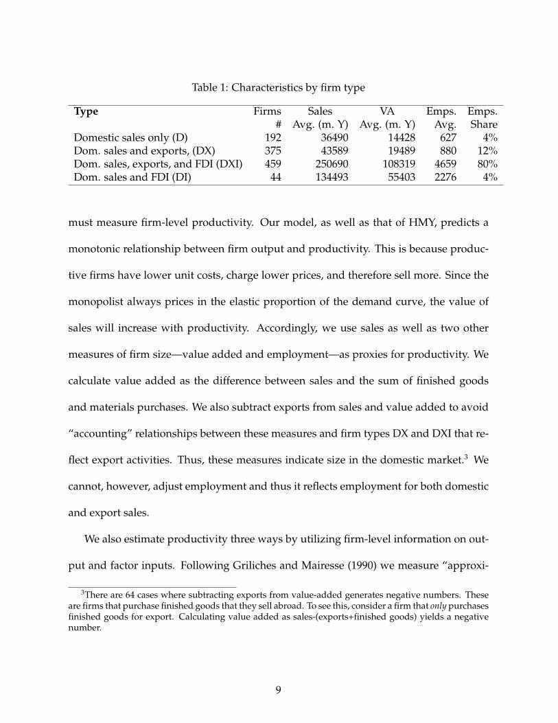
Table 1: Characteristics by firm type

Type Firms Sales VA Emps. Emps.# Avg. (m. Y) Avg. (m. Y) Avg. Share

Domestic sales only (D) 192 36490 14428 627 4%Dom. sales and exports, (DX) 375 43589 19489 880 12%Dom. sales, exports, and FDI (DXI) 459 250690 108319 4659 80%Dom. sales and FDI (DI) 44 134493 55403 2276 4%

must measure firm-level productivity. Our model, as well as that of HMY, predicts a

monotonic relationship between firm output and productivity. This is because produc-

tive firms have lower unit costs, charge lower prices, and therefore sell more. Since the

monopolist always prices in the elastic proportion of the demand curve, the value of

sales will increase with productivity. Accordingly, we use sales as well as two other

measures of firm size—value added and employment—as proxies for productivity. We

calculate value added as the difference between sales and the sum of finished goods

and materials purchases. We also subtract exports from sales and value added to avoid

“accounting” relationships between these measures and firm types DX and DXI that re-

flect export activities. Thus, these measures indicate size in the domestic market.3 We

cannot, however, adjust employment and thus it reflects employment for both domestic

and export sales.

We also estimate productivity three ways by utilizing firm-level information on out-

put and factor inputs. Following Griliches and Mairesse (1990) we measure “approxi-

3There are 64 cases where subtracting exports from value-added generates negative numbers. Theseare firms that purchase finished goods that they sell abroad. To see this, consider a firm that only purchasesfinished goods for export. Calculating value added as sales-(exports+finished goods) yields a negativenumber.

9

mate total factor productivity” as:

ATFP ≡ ln Q/L− s ln K/L.

Intuitively, this productivity measure starts with average labor productivity, Q/L, and

adjusts for capital intensity K/L. Parameter s measures the importance of capital in

the production function and can vary between zero, where productivity equals labor

productivity, and one, where productivity is given by capital productivity (Q/K). In the

empirical implementation we follow Hall and Jones (1999) in setting s = 1/3.

The drawback to ATFP is that it reflects both “true” technical efficiency as well as

scale economies. To see this, consider a Cobb-Douglas production function given by

Q = A[KωL(1−ω)]µ. We can relate our measure of productivity, ATFP, to the true technical

efficiency parameter, denoted A,

ATFP = ln A + (µω − s) ln K + (µ(1− ω)− (1− s)) ln L.

Technical efficiency equals ATFP when µω = s and µ(1 − ω) = 1 − s. This occurs

when there are constant returns to scale (µ = 1) and s equals the true capital cost share,

ω.

Substituting the cost minimization condition s = ω and manipulating, we arrive at

ATFP = (1/µ) ln A +

(µ− 1

µ

)ln Q.

The productivity measure ATFP varies with true technical efficiency and scale. The

10

theory pertains to technical efficiency. Firms with high technical efficiency will export or

invest abroad. Exporting will increase the scale of home operations whereas FDI might

lower it if it displaces production for export. ATFP will be a good measure of technical

efficiency if there are constant returns to scale and s = 1/3 is a reasonable measure of

the cost share of capital.

We also measure productivity by estimating the following four-factor Cobb-Douglas

production function

ln Qit = ln At + βM ln Mit + βK ln Kit + βS ln Sit + βU ln Uit + εit.

where Q is a measure of output and M , K, S, and U , represent materials, capital, skilled

workers, and unskilled workers.

Output is sales minus purchased finished goods. We measure capital as the stock of

depreciable assets (buildings, machinery, and equipment). To allow for heterogeneity

across workers in a firm, we consider two types of labour inputs—production (termed

unskilled, U ) and nonproduction workers (termed skilled, S). We have data on total

compensation paid to each category of employees. We deflate production wages by the

average wage paid to workers with high school degrees in Japan to obtain a measure

of production worker inputs. Similarly, to measure nonproduction worker inputs, we

deflate total salaries of selling, general and administrative (SGA) employees by the av-

erage salary paid to university graduates. We deflate nominal output by the wholesale

price index. Price indices are available at roughly the 2-digit industry level. We de-

flate depreciable assets by the Japanese capital goods deflator. To deflate materials, we

11

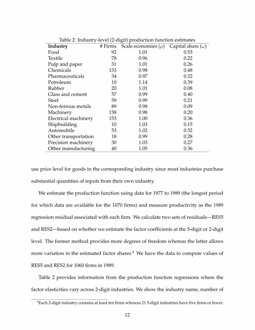
Table 2: Industry-level (2-digit) production function estimatesIndustry # Firms Scale economies (µ) Capital share (ω)Food 92 1.01 0.53Textile 78 0.96 0.22Pulp and paper 31 1.01 0.26Chemicals 133 0.98 0.48Pharmaceuticals 34 0.97 0.32Petroleum 10 1.14 0.39Rubber 20 1.01 0.08Glass and cement 57 0.99 0.40Steel 59 0.99 0.21Non-ferrous metals 89 0.98 0.09Machinery 158 0.98 0.20Electrical machinery 153 1.00 0.36Shipbuilding 10 1.03 0.15Automobile 53 1.02 0.32Other transportation 18 0.99 0.28Precision machinery 30 1.03 0.27Other manufacturing 40 1.05 0.36

use price level for goods in the corresponding industry since most industries purchase

substantial quantities of inputs from their own industry.

We estimate the production function using data for 1977 to 1989 (the longest period

for which data are available for the 1070 firms) and measure productivity as the 1989

regression residual associated with each firm. We calculate two sets of residuals—RES5

and RES2—based on whether we estimate the factor coefficients at the 5-digit or 2-digit

level. The former method provides more degrees of freedom whereas the latter allows

more variation in the estimated factor shares.4 We have the data to compute values of

RES5 and RES2 for 1060 firms in 1989.

Table 2 provides information from the production function regressions where the

factor elasticities vary across 2-digit industries. We show the industry name, number of

4Each 2-digit industry contains at least ten firms whereas 21 5-digit industries have five firms or fewer.

12

firms, the returns to scale (µ = βM +βK +βS +βU ), and capital’s implied share of primary

input costs (ω = βK/(βK + βS + βU ). The data reveal that constant returns to scale is not

a bad assumption as µ ranges from 0.96 to 1.14 and only one industry (petroleum, 10

firms) has a µ that is more than 0.05 away from one. We note that simultaneity is likely

to cause upward bias in estimates of factor shares so these values might be interpreted

as upper limits. Petroleum exhibits the highest returns to scale and Textiles the least.

The average implied capital share of primary inputs is .29 with 11 out of 17 industries

having shares between .20 and .39. There is more variation exhibited when we estimate

the factor shares at the 5-digit industry level, a result partly due less precise estimates.

In these regressions, one industry has µ = .76 whereas it is between .88 and 1.18 for the

remaining 87 industries. Capital’s share of primary inputs has a mean of .33 (coinciden-

tally equal to the value we used for ATFP) but a large standard deviation (.25) once we

remove one 2-firm industry with a capital share of -6.3.5

We are not sure whether to take comfort in what Table 2 reveals about the estimates

of the parameters of the industry production functions. Accounting data do not neces-

sarily correspond well to the underlying economic variables in theoretical production

functions and we must resort to use of book values of capital stocks instead of (usually

unmeasurable) flows of capital services. This may result in inaccurate estimates. On

the positive side, the results of roughly constant returns to scale and capital shares av-

eraging around one-third appear plausible and indicate that ATFP may be a reasonable

approximation.

5While there are no estimated negative factor shares when the coefficients vary at the 2-digit level,negative estimates do occasionally arise for 5-digit industry regressions. None of the negative estimatesare statistically significant when we compute standard errors that allow for correlated errors at the firmlevel.

13

Pavcnik (2002) deals with the endogeneity of input choices using a method due to

Pakes and Olley (1995). Her method also treats potential biases due to non-random

selection of the firm-level sample. This multi-step method uses polynomial approxima-

tions to back out innovations in productivity from the firm’s investment decisions. Our

concern here is not with production function estimation per se but rather with obtain-

ing a measure of productivity that allows us to order firms in an industry. We believe

that standard productivity estimation techniques are adequate for this purpose. In the

analysis that follows, we subtract the industry mean level of productivity from firm pro-

ductivity, a procedure that will alleviate some sources of potential bias in our estimates.

We believe the principle shortcoming of our productivity estimates derives from the

data and cannot be greatly reduced by more complex econometric methods that appear

to make strong identifying assumptions.6

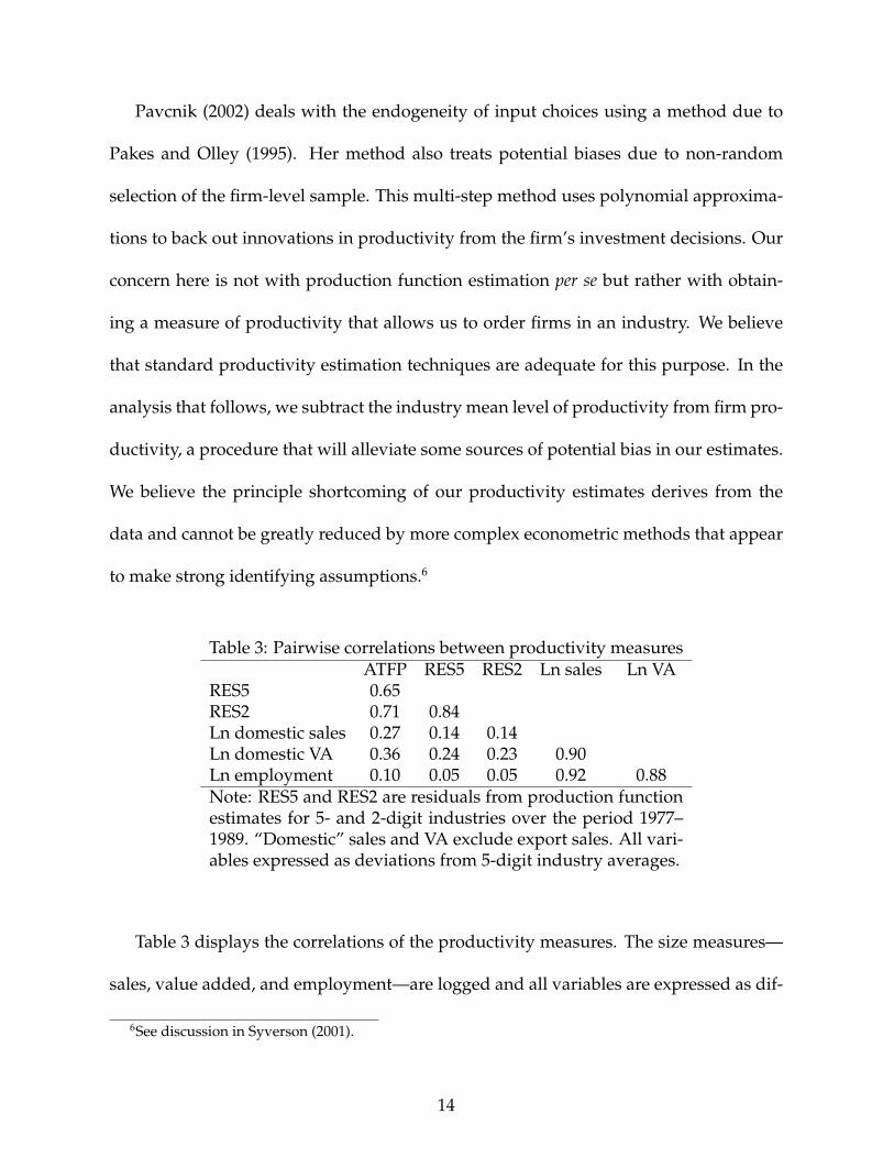
Table 3: Pairwise correlations between productivity measuresATFP RES5 RES2 Ln sales Ln VA

RES5 0.65RES2 0.71 0.84Ln domestic sales 0.27 0.14 0.14Ln domestic VA 0.36 0.24 0.23 0.90Ln employment 0.10 0.05 0.05 0.92 0.88Note: RES5 and RES2 are residuals from production functionestimates for 5- and 2-digit industries over the period 1977–1989. “Domestic” sales and VA exclude export sales. All vari-ables expressed as deviations from 5-digit industry averages.

Table 3 displays the correlations of the productivity measures. The size measures—

sales, value added, and employment—are logged and all variables are expressed as dif-

6See discussion in Syverson (2001).

14

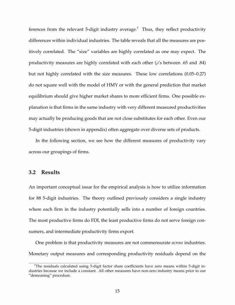
ferences from the relevant 5-digit industry average.7 Thus, they reflect productivity

differences within individual industries. The table reveals that all the measures are pos-

itively correlated. The “size” variables are highly correlated as one may expect. The

productivity measures are highly correlated with each other (ρ’s between .65 and .84)

but not highly correlated with the size measures. These low correlations (0.05–0.27)

do not square well with the model of HMY or with the general prediction that market

equilibrium should give higher market shares to more efficient firms. One possible ex-

planation is that firms in the same industry with very different measured productivities

may actually be producing goods that are not close substitutes for each other. Even our

5-digit industries (shown in appendix) often aggregate over diverse sets of products.

In the following section, we see how the different measures of productivity vary

across our groupings of firms.

3.2 Results

An important conceptual issue for the empirical analysis is how to utilize information

for 88 5-digit industries. The theory outlined previously considers a single industry

where each firm in the industry potentially sells into a number of foreign countries.

The most productive firms do FDI, the least productive firms do not serve foreign con-

sumers, and intermediate productivity firms export.

One problem is that productivity measures are not commensurate across industries.

Monetary output measures and corresponding productivity residuals depend on the

7The residuals calculated using 5-digit factor share coefficients have zero means within 5-digit in-dustries because we include a constant. All other measures have non-zero industry means prior to our“demeaning” procedure.

15

price or unit of measurement of the industry. Employment may vary systematically

across industries as a result of differences in minimum efficient scale. Some type of nor-

malization is necessary before we can aggregate the information across the industries.

Our technique is to subtract of the industry mean for each 5-digit industry so that pro-

ductivity is represented as a difference from the industry average. This procedure forces

each industry to have the same mean productivity (zero).

A second problem results from the limited number of firms in some industries in-

dustry. The number of firms ranges from two to 46. The appendix shows the types of

firms in each industry and reveals that only 15 industries have firms of each type (D,

DX, DXI, DI). Seven industries only have firms of a single type whereas the rest have

two or three types.

To see what issues this heterogeneity raises, consider the fictitious data contained in

Table 4. Each cell corresponds to the average, demeaned productivity level of firms of

the specified type in the specified industry. Assuming the same number of firms in each

cell, average productivity in each industry is zero (as can be seen by summing down

each column). The example follows the productivity ordering predicted by the theory.

Averaging firm types across industries as shown in the last column illustrates two prob-

lems. First, including industry 1 will bias the DXI average towards zero. Second, the

pooling of industries causes DXI average productivity to exceed that of DI firms in this

example.

In light of these issues, we evaluate the theoretical predictions in two ways. Our first

method is to average productivity across industries with the same set of firm types. We

separately examine the 24 industries with DX and DXI firms, the 27 industries with D,

16

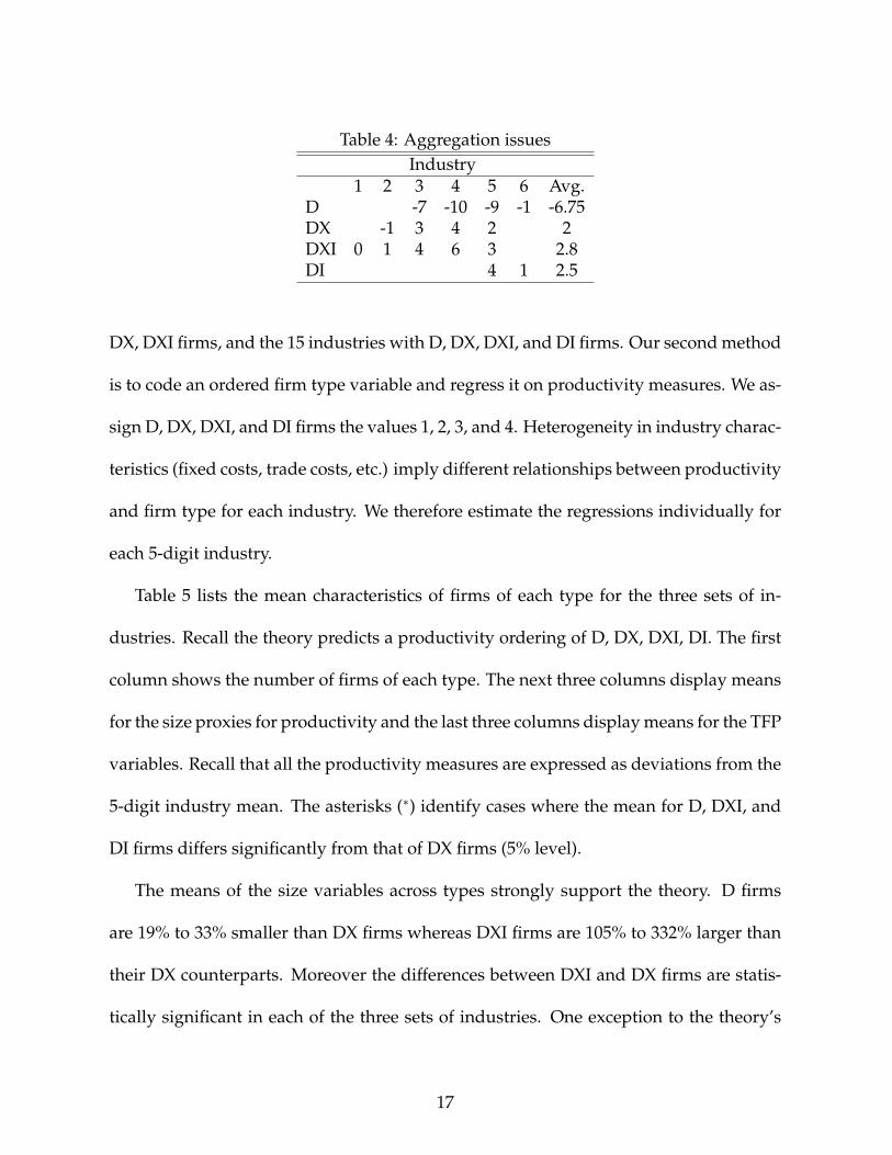
Table 4: Aggregation issuesIndustry

1 2 3 4 5 6 Avg.D -7 -10 -9 -1 -6.75DX -1 3 4 2 2DXI 0 1 4 6 3 2.8DI 4 1 2.5

DX, DXI firms, and the 15 industries with D, DX, DXI, and DI firms. Our second method

is to code an ordered firm type variable and regress it on productivity measures. We as-

sign D, DX, DXI, and DI firms the values 1, 2, 3, and 4. Heterogeneity in industry charac-

teristics (fixed costs, trade costs, etc.) imply different relationships between productivity

and firm type for each industry. We therefore estimate the regressions individually for

each 5-digit industry.

Table 5 lists the mean characteristics of firms of each type for the three sets of in-

dustries. Recall the theory predicts a productivity ordering of D, DX, DXI, DI. The first

column shows the number of firms of each type. The next three columns display means

for the size proxies for productivity and the last three columns display means for the TFP

variables. Recall that all the productivity measures are expressed as deviations from the

5-digit industry mean. The asterisks (∗) identify cases where the mean for D, DXI, and

DI firms differs significantly from that of DX firms (5% level).

The means of the size variables across types strongly support the theory. D firms

are 19% to 33% smaller than DX firms whereas DXI firms are 105% to 332% larger than

their DX counterparts. Moreover the differences between DXI and DX firms are statis-

tically significant in each of the three sets of industries. One exception to the theory’s

17

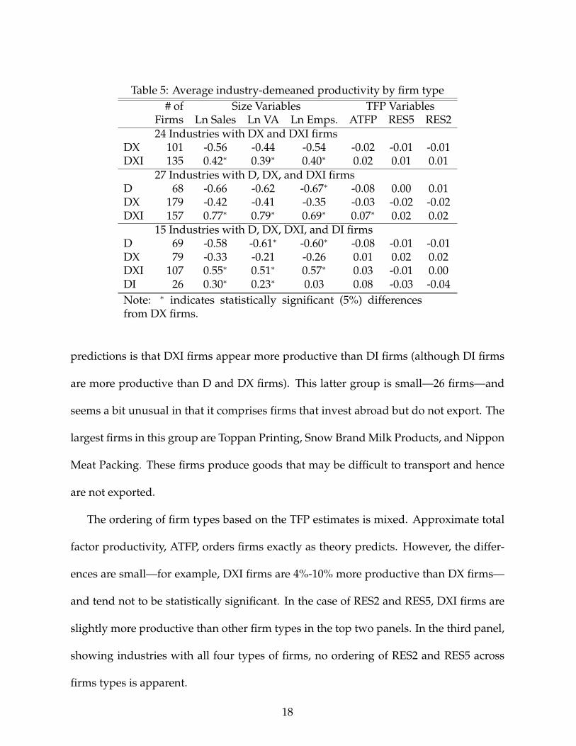
Table 5: Average industry-demeaned productivity by firm type# of Size Variables TFP Variables

Firms Ln Sales Ln VA Ln Emps. ATFP RES5 RES224 Industries with DX and DXI firms

DX 101 -0.56 -0.44 -0.54 -0.02 -0.01 -0.01DXI 135 0.42∗ 0.39∗ 0.40∗ 0.02 0.01 0.01

27 Industries with D, DX, and DXI firmsD 68 -0.66 -0.62 -0.67∗ -0.08 0.00 0.01DX 179 -0.42 -0.41 -0.35 -0.03 -0.02 -0.02DXI 157 0.77∗ 0.79∗ 0.69∗ 0.07∗ 0.02 0.02

15 Industries with D, DX, DXI, and DI firmsD 69 -0.58 -0.61∗ -0.60∗ -0.08 -0.01 -0.01DX 79 -0.33 -0.21 -0.26 0.01 0.02 0.02DXI 107 0.55∗ 0.51∗ 0.57∗ 0.03 -0.01 0.00DI 26 0.30∗ 0.23∗ 0.03 0.08 -0.03 -0.04Note: ∗ indicates statistically significant (5%) differencesfrom DX firms.

predictions is that DXI firms appear more productive than DI firms (although DI firms

are more productive than D and DX firms). This latter group is small—26 firms—and

seems a bit unusual in that it comprises firms that invest abroad but do not export. The

largest firms in this group are Toppan Printing, Snow Brand Milk Products, and Nippon

Meat Packing. These firms produce goods that may be difficult to transport and hence

are not exported.

The ordering of firm types based on the TFP estimates is mixed. Approximate total

factor productivity, ATFP, orders firms exactly as theory predicts. However, the differ-

ences are small—for example, DXI firms are 4%-10% more productive than DX firms—

and tend not to be statistically significant. In the case of RES2 and RES5, DXI firms are

slightly more productive than other firm types in the top two panels. In the third panel,

showing industries with all four types of firms, no ordering of RES2 and RES5 across

firms types is apparent.

18

Table 6: Ordered Type RegressionsProductivity Measure # Positive # Negative Stacked

A B CLn Sales 75 6 0.325

(32) (0) (0.023)Ln VA 69 9 0.289

(25) (0) (0.025)Ln emps 73 8 0.344

(35) (0) (0.023)ATFP 53 28 0.317

(7) (0) (0.075)RES5 50 31 0.051

(0) (2) (0.157)RES2 49 32 0.062

(2) (2) (0.137)Note: Numbers in parenthesis report the number of t val-ues greater than 2 in columns A and B and standard errorsin column C.

Table 6 summarizes the results of the ordered type regressions where the dependent

variable assigns values of 1–4 to the firm types D, DX, DXI, and DI. The explanatory

variables are the alternative measures of productivity. These regressions could be es-

timated using ordered probit. This would have the desirable feature of allowing each

firm type to obtain its own cutoff parameter. However, many of our industries do not

have a sufficient number of firms to obtain reliable estimates of the coefficient on pro-

ductivity while simultaneously estimating multiple cutoff parameters. Therefore, we

use ordinary least squares which can be interpreted as a linear probability model.

The first column of Table 6 shows the number of cases where we estimate a posi-

tive coefficient on the productivity variable. The number of significant (at 5% level in a

two-sided t test) positive coefficients is shown directly underneath in parentheses. The

second column provides corresponding information for negative coefficients. The re-

19

sults for the size variables (sales, value added, and employment) strongly support the

theory. The vast majority of the estimates are positive and many are significant. Neg-

ative estimates, when they obtain, are never significant. The evidence is much more

mixed for the TFP variables (ATFP, RES5, and RES2). While the estimates tend to be

positive, they are rarely significant and occasional negative and significant estimates

obtain. The last column shows results where we stack industries and estimate a single

coefficient for productivity with standard errors listed in parenthesis. The estimates are

positive, significant and similar in magnitude for sales, value added, employment, and

ATFP. The estimates for RES5 and RES2 are positive but much smaller and statistically

insignificant.8

Overall, we find some support for the predictions of the theory with the results for

the size proxies being much stronger than those for the productivity estimates. Firms

that only serve the domestic market tend to be less productive than firms that export

and firms that do FDI. Investors who also export are generally more productive than

exporters who do not have overseas investment. The theory suggests that firms that

have overseas investment but no exports should be most productive. This prediction

is not supported. What we have referred to as “the theory” is actually a special case of

a more general model. In the next section we show that relaxing key assumptions can

lead to quite different predicted orderings.

8Estimates of the stacked ordered type regressions using ordered probit gave a very similar pattern oft statistics for the different size and TFP variables.

20

4 Extending the Model

The previous analysis assumed equal wages in the home and foreign market, thus negat-

ing any “factor-seeking” motive for FDI. It also abstracted from considering the home

market by assuming that the firm maintains its home plant to serve home-country con-

sumers. In this section we investigate how robust the theoretical predictions are to these

assumptions. We begin by considering wages differences across countries. Then we al-

low for the possibility of shutting down the home plant and using the foreign plant to

serve home consumers.

4.1 Wage differences

The productivity of investing firms exceeds that of exporting firms because, as shown

in Figure 1, the FDI profit function is lower than the export profit function for low pro-

ductivity levels but rises more quickly with increases in productivity. As shown in the

paper, with identical marginal costs (equal to w) these profits functions are:

πX = [(1− w/A− τ)/2]2,

πI = [(1− w/A)/2]2 −K.

The ratio of the slope of the FDI profit function, ∂πI/∂A, to the slope of the export profit

function, ∂πX/∂A, exceeds one:

1− w/A

1− w/A− τ> 1.

21

An intersection of the ΠX(A) and ΠI(A) curves must exist since profits of FDI rise faster

than profits of exporting as productivity increases as long as the fixed costs of FDI make

ΠI(A) < ΠX(A) for low A. Now consider different wage costs in the foreign country

equal to wf = wh + ε. The ratio of the slopes can now be expressed as

[1− wh/A− ε/A

1− wh/A− τ

] [wh + ε

wh

].

For FDI to be the desired alternative for any productivity level, ε/A must be less than

τ (given a positive fixed cost of FDI, the marginal cost disadvantage associated with

producing abroad, ε/A, must be smaller than the per unit transport cost savings of FDI,

τ ). Inspection reveals that for 0 < ε < Aτ , the ratio of the slopes exceeds one. However,

for ε < 0 the ratio may fall below one, thereby admitting the possibility of multiple

intersections of the profit functions. Thus, as long as the foreign wage is no lower than

the home wage, the result that investors are more productive than exporters holds under

the assumption that the home plant continues to operate.

4.2 Single-plant operations

If the fixed costs of operating a plant are high and production costs are low in the for-

eign country, a firm will prefer to close its home plant and serve its home customers

by importing from the foreign plant. For example, Sony could produce televisions in

a low-wage country such as Malaysia and shut down television production in Japan.

In this section, we consider this possibility and its implications for firms with different

productivity levels.

22

In general, the location of the single plant (in the home or foreign country) depends

on relative costs and market sizes in each country. All firms prefer to locate in a low-

cost country that has a large market. Thus, the interesting cases occur when one country

offers a large market and another country offers low production costs (wages). Firms

with different productivity levels may evaluate this tradeoff differently.

We define three alternative configurations of international production. Strategy H

denotes single-plant production in the home market with exports to the foreign coun-

try. Strategy R (replication) involves production in both countries. Each plant serves

local consumers and no exporting occurs. These are the two strategies we have already

considered. The third strategy, F , entails production in the foreign country with exports

back to the home country to serve consumers there. Firms prefer F when fixed costs of

production are high and the foreign country offers a large market or low wages. The

decision to access low costs abroad may be termed factor-seeking FDI. Strategies R and

F both involve investment abroad whereas strategy H involves exporting from home.

To allow for differences in market size, we consider Mh consumers in the home coun-

try and Mf consumers in the foreign country, each with demand q = 1 − p. Wages at

home and abroad are wh and wf . Fixed costs are Kh and Kf .

As before, we assume that productivity transfers to foreign operations. The profit

functions associated with each strategy are

ΠH = Mh[(1− wh/A)/2]2 + Mf [(1− wh/A− τ)/2]2 −Kh,

ΠF = Mh[(1− wf/A− τ)/2]2 + Mf [(1− wf/A)/2]2 −Kf ,

23

ΠR = Mh[(1− wh/A)/2]2 + Mf [(1− wf/A)/2]2 −Kh −Kf .

Firms choose the strategy that yields the highest profits and the choice depends on rel-

ative market sizes, marginal production costs, transport costs, and fixed costs. We are

interested in whether our previous result that more productive firms choose FDI contin-

ues to hold.

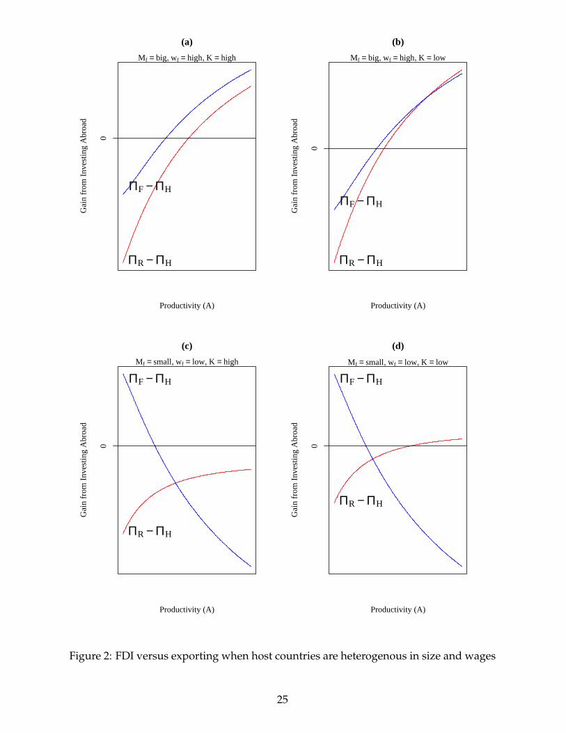
We illustrate different outcomes in Figure 2. Since there is no interaction between

fixed costs and productivity in the model, we set Kh = Kf = K.9 In order for the

smaller of the two countries to be competitive, it must offer lower wages. The top two

panels consider the case where the foreign market is big, but high cost. The lower panels

depict the case where the foreign market offers low costs, but a small market. The two

left panels assume high fixed costs (K = .05) relative to the situation depicted in the

right panels (K = .045).10 The vertical axis measures the profits of FDI less the profits of

home production. FDI can involve two-plant production (R) or single-plant production

abroad and exports back to home (F ). Each panel contains two curves that plot the R

or F profits minus H profits for different levels of productivity. The firm chooses the

more profitable FDI alternative unless both are negative, in which case, a firm prefers

H , home production and exporting.

The top panels show that high productivity firms prefer FDI to exporting from home

when foreign wages are high. We already established the result depicted by the ΠR−ΠH

curve in the two figures when we showed the (replication) FDI profit function rises more

9Differences in fixed costs would not affect the relative incentive for firms with different productivityto choose one strategy or another.

10To generate the figures, we assume that transport costs equal .1, the larger country has M = 2 andw = 1, and the smaller country has M = 1 and w = .9.

24

(a)

Productivity (A)

Gai

n fr

om In

vest

ing

Abr

oad

0

ΠF − ΠH

ΠR − ΠH

Mf = big, wf = high, K = high

(b)

Productivity (A)G

ain

from

Inve

stin

g A

broa

d

0

ΠF − ΠH

ΠR − ΠH

Mf = big, wf = high, K = low

(c)

Productivity (A)

Gai

n fr

om In

vest

ing

Abr

oad

0

ΠF − ΠH

ΠR − ΠH

Mf = small, wf = low, K = high

(d)

Productivity (A)

Gai

n fr

om In

vest

ing

Abr

oad

0

ΠF − ΠH

ΠR − ΠH

Mf = small, wf = low, K = low

Figure 2: FDI versus exporting when host countries are heterogenous in size and wages

25

quickly than the exporting profit function as productivity increases. This implies that

high productivity firms are more likely to engage in replication FDI and the figures bear

this out. We have not previously considered, however, the possibility of shutting down

the home plant. The ΠF −ΠH curve shows that this is more profitable than H for highly

productive firms. In this case, the productive firms find it relatively more desirable to

locate in the large market even at the expense of higher production costs. In the left

panel, high fixed costs make single-plant production dominate two-plant production

for all productivity levels. In the right panel, the most productive firms choose R over

F .

The lower two panels show that the results change dramatically when the foreign

market is low cost. In the left panel, we set fixed costs at a high enough level to make

replication undesirable regardless of firm productivity. The panel shows that F can

be more profitable than H but only for the least productive firms. These firms find it most

attractive to take advantage of low costs abroad at the expense of incurring trade costs to

serve the large market. In the right panel, fixed costs are low enough to make replication

the preferred strategy for highly productive firms. Here the least and most productive

firms choose FDI, with the least productive firms choosing F and the most productive

firms choosing R.

4.3 Testing an implication of the extended model

Figure 2 indicates that the type of firm that chooses FDI depends on characteristics of

the host country. When the host country offers a large market but has high wages, un-

productive firms are unlikely to choose FDI. However, when the foreign country offers

26

● ●● ●

4060

8010

012

0

(a)

Quartiles of Productivity

Hos

t Inc

ome

as %

of J

apan

's

1 2 3 4

●●

●

●

4060

8010

012

0

(b)

Quartiles of Employment

1 2 3 4

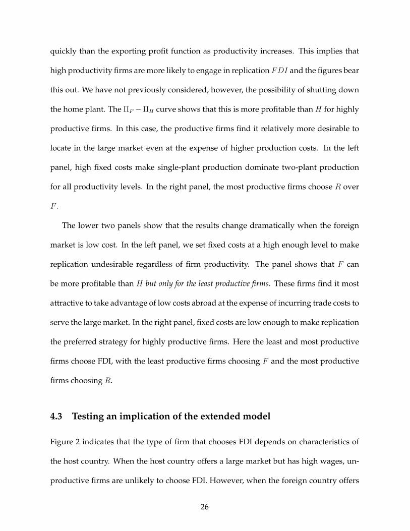
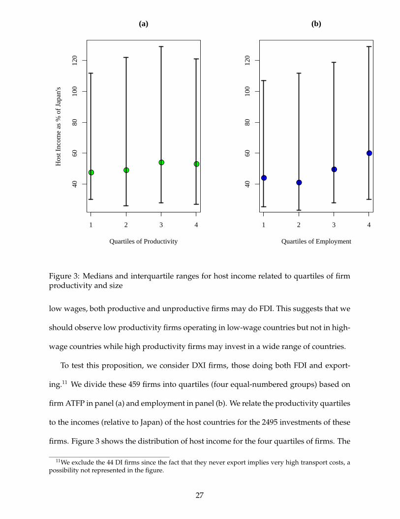
Figure 3: Medians and interquartile ranges for host income related to quartiles of firmproductivity and size

low wages, both productive and unproductive firms may do FDI. This suggests that we

should observe low productivity firms operating in low-wage countries but not in high-

wage countries while high productivity firms may invest in a wide range of countries.

To test this proposition, we consider DXI firms, those doing both FDI and export-

ing.11 We divide these 459 firms into quartiles (four equal-numbered groups) based on

firm ATFP in panel (a) and employment in panel (b). We relate the productivity quartiles

to the incomes (relative to Japan) of the host countries for the 2495 investments of these

firms. Figure 3 shows the distribution of host income for the four quartiles of firms. The

11We exclude the 44 DI firms since the fact that they never export implies very high transport costs, apossibility not represented in the figure.

27

circles represent medians and the extensions show the 25th and 75th percentiles of the

data.

We find some support for the extended version of the model. While interquartile

ranges of host income are large for all quartiles of productivity, median and third-

quartile host incomes tend to rise in step with productivity. The relationship is stronger

for employment than ATFP. Small firms only rarely invest in countries with higher in-

comes than Japan. The figure corroborates the theory’s prediction that productive firms

invest in a wider range of host countries.

5 Conclusion

In this paper we have investigated why firms in the same industry select different modes

to reach foreign customers. Our paper complements the work of Helpman, Melitz, and

Yeaple in three ways. First, we provide a very simple alternative model that yields the

same predicted relationship between productivity and the decision to export or invest

abroad. Second, we relax the assumption of equal wages and find that the productiv-

ity ordering can be reversed when the foreign market is the low-cost production site.

Finally we examine productivity orderings using a sample of 1070 Japanese manufac-

turing firms.

Our empirical work shows that the relationship between productivity and the FDI

versus export decision depends very much on the proxy used to measure productiv-

ity. Firm size measures exhibit a consistent ordering: firms that export are larger than

firms that just serve the domestic market, but both types are smaller on average than

28

firms that invest abroad as well as export. Production function residuals yield much

weaker relationships with firm type. Orderings vary across samples and differences are

uniformly small.

We find that heterogeneity in firm productivity appears to interact in important ways

with heterogeneity in the market size and factor prices of potential host countries. These

interactions underscore the importance of simultaneous consideration of firm and host-

country differences in research on the FDI versus export decision.

29

Appendix: Industry information

Industry (5-digit) # Firms Median Emps. # D # DX # DXI # DIFoodFeed 5 472 4 0 0 1Sugar 9 133 5 2 0 2Flour 8 329 5 2 0 1Oil 8 168 6 0 2 0Alcohol 9 1818 1 3 4 1Confections/Bread 16 1436 8 3 2 3Ham 6 3620 2 0 0 4Spice/Condiments 10 694 4 1 4 1Dairy 6 3516 1 0 2 3Other Food 16 903 10 0 4 2TextileSynthetics 6 5404 0 1 5 0Cotton 19 2225 5 3 11 0Silk 7 133 3 0 4 0Wool 9 426 4 1 2 2Processed 16 407 4 7 5 0Other Textiles 23 495 5 9 8 1Pulp & PaperMajor Paper 5 5142 0 1 4 0Pulp Paper 26 634 10 9 6 1ChemicalsMajor Chemical 7 5295 0 1 6 0Fertilizers 5 554 1 4 0 0Soda/Chlorine 7 2161 0 3 4 0Petrochemicals 2 3598 0 0 2 0Synthetic Resin 25 865 2 10 11 2Oxygen 8 617 2 3 3 0Soap/Detergent 8 779 0 3 5 0Cosmetics/Toothpaste 4 1952 1 0 3 0Paint & Ink 15 728 0 1 10 4Agric. Chems. & Pesticides 6 617 1 1 4 0Other Chemicals 46 568 3 27 16 0PharmaceuticalsMajor Pharma. 5 5979 0 0 5 0Prescriptions 20 2046 4 9 7 0Non-prescriptions 9 526 2 5 2 0PetroleumRefinery 7 2412 2 4 1 0Coal/Petrolum Products 3 307 1 2 0 0RubberTires 7 3556 2 0 5 0Other Rubber 13 848 2 6 5 0

30

Industry (5-digit) # Firms Median Emps. # D # DX # DXI # DIGlass & CementGlass 7 1565 2 3 2 0Cement I 7 1646 2 1 3 1Cement II 14 467 8 0 5 1Ceramics 11 681 2 4 5 0Bricks 11 441 0 6 5 0Carbon & Others 7 477 0 4 3 0SteelIntegrated Steel 8 20121 0 2 6 0Electric Mills 14 561 3 6 5 0Special Steel 7 2855 0 4 3 0Amalgamated Steel 5 674 0 4 1 0Alloy Steel 20 470 4 10 5 1Stainless Steel 5 1546 0 3 2 0Non-Ferrous MetalMajor Refining 8 3130 0 1 7 0Other Metals 5 538 1 2 1 1Aluminum 11 615 3 2 6 0Electric Wires & Cables 14 883 1 6 7 0Construction Metals 14 576 7 6 1 0Other Non-Ferrous Metals 38 567 11 15 11 1MachineryMachine Tools 30 756 2 14 14 0Press Machines 3 551 0 2 1 0Textile 10 645 0 8 2 0Trans.,Construc. & Combus. 24 852 1 14 9 0Agriculture 7 703 2 3 2 0Chemicals 35 606 1 20 14 0Sewing Machines/Looms 4 2830 0 1 3 0Rod Production Machinery 12 1860 0 4 8 0Office 4 1089 1 1 2 0Other Machinery 29 543 6 15 8 0Electrical MachineryGeneral Electronics 4 58447 0 0 4 0Turbines 16 1275 0 7 9 0Household Electronics 29 1978 0 3 26 0Communication 30 1429 0 17 13 0Electrical Parts 24 1067 1 4 18 1Control Machinery 16 908 4 7 5 0Battery 5 1287 0 2 3 0Auto-related 4 4294 0 0 4 0Other Electrical Machinery 26 992 6 7 11 2Shipbuilding 10 3199 0 5 5 0

31

Industry (5-digit) # Firms Median Emps. # D # DX # DXI # DIAutomobileAutomobiles 13 12616 1 2 10 0Parts 35 1949 6 3 19 7Body/Others 5 5103 0 2 3 0Other TransportationVehicles, Rolling Stocks 4 1885 0 4 0 0Bicycles 5 225 1 3 1 0Other Transportation 9 808 2 2 5 0Precision MachineryClocks/Watches 5 1388 0 2 3 0Camera 8 3125 0 0 8 0Measuring Instruments 17 817 0 11 6 0Other ManufacturingPublishing 8 917 4 1 2 1Musical Instruments 2 8215 0 0 2 0Construction Material 7 288 6 1 0 0Office Supplies 6 1126 0 4 2 0Other Manufacturing 17 800 4 6 7 0

32

References

Bernard, Andrew B. and J. Bradford Jenson, 1999, “Exceptional Exporter Performance:Cause Effect, or Both?” Journal of International Economics 47:1–25.

Bernard, Andrew B., Jonathan Eaton, J. Bradford Jenson, Samuel Kortum, 2003, “Plantsand Productivity in International Trade,” American Economic Review 93(4):1268–1290.

Brainard, S. Lael, 1997, “An Empirical Assessment of the Proximity-ConcentrationTradeoff Between Multinational Sales and Trade,” American Economic Review 87(4):520–544.

Girma, Sourafel and Richard Kneller, 2003, “Export versus FDI: An Empirical Test,”manuscript.

Griliches, Zvi and Jacques Mairesse, 1990, “R&D and Productivity Growth: ComparingJapanese and U.S. Manufacturing Firms,” Hulten, Charles, ed., Productivity Growthin Japan and the United States, Chicago: The University of Chicago Press.

Hall, Robert, and Charles Jones, 1999 “Why do Some Countries Produce So Much MoreOutput per Worker than Others?,” Quarterly Journal of Economics, 83-116.

Helpman, Elhanan, Marc J. Melitz, and Stephen R. Yeaple, forthcoming, “Export versusFDI with Heterogeneous Firms,” American Economic Review and NBER WorkingPaper No. 9439.

Melitz, Marc J., forthcoming, “The Impact of Trade on Intra-Industry Reallocationsand Aggregate Industry Productivity,” Econometrica and NBER Working Paper No.8881.

Pakes, Ariel, and Steven Olley, 1995, “A Limit Theorem for a Smooth Class of Semi-parametric Estimators,” Journal of Econometrics 65, 295–332.

Pavcnik, Nina, 2002, “Trade Liberalization, Exit, and Productivity Improvements: Evi-dence from Chilean Plants,” The Review of Economic Studies 69, 245–76.

Syverson, Chad, 2001, “Market Structure and Productivity: A Concrete Example” Uni-versity of Chicago, manuscript.

Toyo Keizai, Inc., 1992, Japan Overseas Investment: A Complete Listing by Firms and Coun-tries 1992/93, Tokyo.

33