Subsidies for FDI:

Implications from a Model with Heterogeneous Firms∗

Davin Chor†

Singapore Management University

First version: February 2006This version: January 2009

Comments welcome

Abstract

This paper analyzes the welfare effects of subsidies to attract multinational corporations when firmsare heterogeneous in their productivity levels. I show that the use of a small subsidy raises welfare inthe FDI host country, with the consumption gains from attracting more multinationals exceeding thedirect cost of funding the subsidy program through a tax on labor income. This welfare gain stemsfrom a selection effect, whereby the subsidy induces only the most productive exporters to switch toservicing the host’s market via FDI. I further show that for the same total subsidy bill, a subsidy tovariable costs delivers a larger welfare gain than a subsidy to the fixed cost of conducting FDI, since avariable cost subsidy also raises the inefficiently low output levels stemming from each firm’s markuppricing power.

Keywords: FDI subsidies; heterogeneous firms; fixed versus variable cost subsidies; import subsidies.

JEL Classification: F12, F13, F23, L23

∗I thank Pol Antras, Elhanan Helpman, Edwin L.-C. Lai, and Marc J. Melitz for their comments and patient advice, aswell as the editor, Jonathan Eaton, and referees for their helpful suggestions. I have also benefited from comments fromPao-Li Chang, Hian Teck Hoon, Jang Ping Thia, seminar participants at the international lunch at Harvard, the 2006Society for Economic Dynamics Annual Meeting (Vancouver), and Singapore Management University. Financial supportfrom the Institute for Humane Studies is gratefully acknowledged. All errors are my own.†School of Economics, Singapore Management University, 90 Stamford Rd, Singapore 178903. Tel: +(65) 6828-0876.

Fax: +(65) 6828-0833. E-mail: davinchor@smu.edu.sg

1

1 Introduction

This paper presents an application of the trade models with heterogeneous firms advanced by Melitz

(2003) and Helpman et al. (2004) to an analysis of policy interventions related to foreign direct investment

(FDI). It examines the welfare implications of subsidies to attract multinational corporations (MNCs) in

a setting where firms in the target industry are heterogeneous in their productivity levels.

FDI subsidies have become increasingly common, with many countries now keen to attract MNCs to

their shores for a variety of reasons. At a basic level, there is typically a direct consumption gain: The

relocation of production lowers the prices that MNCs charge in the host country’s market, due to the

savings on cross-border transport costs and possibly also labor costs (if the host country features lower

wages). In addition, countries often value the foreign capital or employment creation that MNCs bring.

The arguments for FDI have further highlighted other benefits for economic growth, such as industry

spillovers and technology transfers, although these have been more difficult to identify empirically.1

Not surprisingly, countries that hold such positive views towards FDI have used an array of incentive

measures to try to attract a larger share of the FDI pie, including tax holidays, job-creation subsidies, and

even the construction of industrial facilities. A recent edition of the World Investment Report surmised

that “[t]he use of locational incentives to attract FDI has considerably expanded in frequency and value”

(UNCTAD, 2003, p.124), resulting in an intense competition among countries for FDI projects.2 That

said, it is not immediately apparent that such policies necessarily raise welfare in the host country, even

in the absence of strategic competition for FDI. On net, the fiscal costs of such subsidies have to be

weighed against the benefits of an increased multinational presence.

In this paper, I assess this tradeoff formally in a two-country model with heterogeneous firms. I

consider a Home country where multinationals are headquartered and a Foreign country seeking to

attract FDI. Firms differ in their innate productivity levels, which are independent draws from a pre-

existing distribution of technological possibilities. The initial industry equilibrium sees only the most

productive Home firms conducting horizontal FDI in Foreign to service that market, since only these

firms can afford the high fixed costs of operating an overseas plant. I then examine how welfare in the

foreign host country is affected when it offers a FDI subsidy: Focusing on the consumption gains from

attracting more MNCs, do these gains to the host country outweigh the direct cost of financing the

subsidy scheme through a tax on its workers? Of note, the model that I formulate admits a closed-form

expression for consumer welfare, making the analysis of these policy interventions tractable.1For example, Aitken and Harrison (1999) find only small net effects of FDI on domestic firms in Venezuela. On the other

hand, Javorcik (2004) presents evidence of positive spillovers in Lithuania on the productivity of local suppliers. Haskel etal. (2007) find positive effects of a greater foreign presence on domestic plant productivity in the UK, although they arguethat the value of the gains from these spillovers is smaller than the quantum of subsidies reportedly extended to MNCs. Seealso Wells et al. (2001) who contend that tax incentives to attract FDI failed to deliver net gains in Indonesia.

2For example, there is brewing unease among some Western European countries over the aggressive use of corporate taxcuts by several Central and Eastern European countries, such as Poland and Slovakia, to attract foreign corporations (TheEconomist, July 24th, 2004). See Hines (1996) and Devereux and Griffith (1998) for evidence that differences in corporatetax rates help to explain the cross-state or cross-country variation in volumes of MNC activity.

2

Previewing the results in Section 3, I establish that a small FDI subsidy indeed delivers a welfare

improvement for the host country. This holds both for a subsidy that reduces MNCs’ fixed costs of

operation (such as the construction of industrial parks and infrastructure) and for a subsidy that is

applied to their variable costs of production (such as corporate tax rate cuts or job-creation subsidies).

Importantly, this welfare gain stems from a selection effect that arises when firms are heterogeneous: The

subsidy attracts only the most productive Home firms that were initially servicing the Foreign market

via exports to switch to horizontal FDI instead. Being relatively productive, this margin of firms already

sets lower prices in the initial equilibrium. With the switch to FDI, the consumption gains in Foreign

from the savings on transport costs are thus large, since the subsequent price reduction is applied over a

large volume of consumption. At the same time, to ensure that these consumption gains actually exceed

the funding cost of the policy, one also requires that the mass of MNCs be relatively small, in order to

cap the size of the subsidy bill. This translates neatly in the model into an analytic condition governing

the degree of firm heterogeneity, specifically that the distribution of firm productivities not display too

thick a right-tail; reassuringly, this is a condition found to be readily satisfied in the estimates of firm

productivity distributions in Helpman et al. (2004).

The key role played by firm heterogeneity and the selection effect for these welfare results is made

clear in Section 3.3, where I show that the scope for a net gain from a FDI subsidy is theoretically

ambiguous when all firms are instead identical, as in the antecedent model of Krugman (1980). When

all firms share the same productivity level, a subsidy that induces one firm to switch from exports to

FDI necessarily induces all Home firms to make the same decision. This generates a large subsidy bill,

which can more than negate the consumption gains if the fixed cost of conducting FDI is high or if the

productivity level of Home firms is low, so that a large per-firm subsidy is needed. In addition to this

selection effect, a varieties effect emerges when we take into account how the subsidy raises the ex ante

profitability of potential entrants to the Home industry. Section 3.4 shows that this increases the number

of Home varieties and amplifies the welfare gain to Foreign in the full industry equilibrium.

I explore quantitatively some properties of the host country welfare function in Section 3.5. In

particular, I illustrate how the optimal subsidy varies in response to shifts in the structural parameters

of the model, such as the degree of firm heterogeneity and the industry cost parameters. These exercises

also highlight a key difference between fixed and variable cost subsidies, namely that the latter have

a much larger impact on the host country’s welfare. Indeed, I establish formally in Section 3.6 that a

variable cost subsidy delivers a greater welfare gain than a fixed cost subsidy that incurs the same total

subsidy bill, subject to a mild sufficient condition. Intuitively, a variable cost subsidy further prompts

each MNC to raise output levels, delivering an additional kick to consumption by counteracting some of

the inefficiency arising from firms’ markup pricing power.

This paper contributes to an extensive literature on the welfare effects of FDI subsidies, presenting

a first attempt (to the best of my knowledge) at applying a framework with heterogeneous firms to this

3

policy issue. The model has the advantage that it allows us to be very precise in describing the behavior

of individual firms in the industry equilibrium, specifically how each firm’s productivity draw and the

size of the FDI subsidy jointly pin down whether it can profitably enter the Foreign market, and if so, its

optimal mode for servicing that market (exports versus FDI). The comparison of fixed versus variable

cost subsidies is a natural question to investigate with this model, yet this is a question that has been

under-explored despite the observation that FDI subsidies can assume diverse forms.

Separately, this paper speaks to a broader literature on optimal policy towards foreign investment.

The early theoretical contributions here, by MacDougall (1960), Kemp (1966) and Jones (1967), focused

on analyzing the jointly optimal levels of commodity tariffs and capital flow taxes in a two-factor world

where only one factor (capital) is internationally mobile. In this strand of work however, FDI is viewed

as synonymous with capital movements, in contrast to the more recent literature on MNCs which treats

FDI more concretely as the production activities of overseas affiliates. Along these latter lines, there has

been much work exploring economic settings in which FDI subsidies might lead to a welfare improvement.

For example, Haaland and Wooten (1999) examine how FDI subsidies can foster agglomeration effects.3

Pennings (2005) shows that a subsidy is optimal when foreign investors face uncertainty over demand

conditions in the host economy. Others have argued that FDI subsidies can help to alleviate the under-

provision of public services (Black and Hoyt, 1989), or improve the allocation of firms’ production facilities

to countries from the standpoint of aggregate efficiency (Fumagalli, 2003).

In this paper, the welfare improvement stems instead from the reduction of barriers to entry into

the host country market, specifically for the most productive Home firms that would have serviced the

Foreign market via exports in the absence of the FDI subsidy. I focus on the consumption gains accruing

to the host country from attracting more MNCs, namely the benefit from accessing MNCs’ products

more cheaply due to the savings on transport costs. While this puts aside other potential benefits such

as technology spillovers, agglomeration effects, or an increased labor demand, the model nevertheless

provides a useful benchmark, since such additional effects would intuitively reinforce the gains from

attracting FDI. The results I derive are closely related to recent work by Demidova and Rodriguez-Clare

(2008), who demonstrate how a simple consumption subsidy, import tariff, or export tax can offset the

markup pricing distortion in a Melitz-type model to achieve the first-best welfare level (although there

are key differences between their production setting and that in this paper; see Section 4.1 below).

The paper proceeds as follows. Section 2 describes the building blocks of the model. Section 3

establishes the main propositions on the welfare gain from either a fixed or variable cost subsidy to FDI.

Section 4 explores two extensions. A parallel analysis shows that there is a similar scope for improving3Haufler and Wooten (1999), Ottaviano and van Ypersele (2005), and Baldwin and Okubo (2006) discuss how market

size can confer countries with an advantage in attracting firms or mobile capital. Baldwin and Okubo (2006) in particularintroduce firm heterogeneity in a two-country new economic geography model with footloose firms who can choose whereto base their headquarter operations after observing their productivity draw. In their model, a subsidy from the smallerSouthern country might attract some firms to relocate their Northern headquarters, although the question of the net welfareeffect on the South remains to be explored.

4

welfare in Foreign through an import subsidy (Section 4.1), and I discuss how this result relates to

Demidova and Rodriguez-Clare (2008). I also confirm the robustness of the results under an alternative

utility specification that incorporates richer income effects (Section 4.2). Section 5 concludes. Detailed

proofs are in a supplementary Appendix available on the author’s website, or upon request.

2 A Two-Country Model with Heterogeneous Firms

There are two countries, Home and Foreign, indexed by H and F respectively. Each economy is made

up of two sectors: (i) a homogeneous good sector (the domestic numeraire), and (ii) a (country-specific)

differentiated goods sector. Labor is the sole factor of production, assumed to be immobile across borders.

Utility: The utility of the representative consumer in country i is given by:

Ui = x0i +

∑c=H,F

1µ

(Xci )µ (1)

Here, x0i denotes consumption of the homogeneous (background) good. Xc

i is the familiar Dixit-Stiglitz

aggregator of consumption over products, xci , from country c’s differentiated goods sector, given by:

Xci =

[∫Ωcixci (a)αdGc(a)

] 1α , where Ωc

i is the set of products from country-c firms available to consumers

in country i. (For example, when c = H and i = F , ΩHF is the union of the set of goods exported from

Home to Foreign and the set of goods produced in Foreign by Home MNCs.) I assume that 0 < µ < α < 1,

so the differentiated products are pairwise substitutes; moreover, products from the same country are

closer substitutes than products drawn from different countries. Differentiated products are indexed by

a, which is the amount of labor required to produce one unit of output. 1/a is thus the firm’s labor

productivity. Upon paying the fixed cost of entry into the industry, each firm draws its a from a pre-

existing technological distribution, Gc(a). The resulting productivity differences are the key dimension

along which firms in this sector are heterogeneous.

The utility function in (1) is maximized with respect to the budget constraint:

x0i +

∑c=H,F

∫Ωci

pci (a)xci (a)dGc(a) = wi (2)

where wi is the wage income of a representative consumer in country i, and pci (a) is the unit price of

product xci (a). The background good x0i is produced with a constant returns to scale technology and

its price is normalized to 1. Solving the consumer maximization problem yields a demand function for

each product with constant elasticity, ε = 11−α > 1, given by: xci (a) = (Xc

i )µ−α1−α pci (a)−ε. Note that I have

focused the analysis here on equilibria in which there is a strictly positive amount of production and

consumption of the background good in each country (x0i > 0); this holds for example when the labor

force in each country is sufficiently large. I will show in the numerical exercises in Section 3.5 that this

positive employment condition for the background sector is not particularly restrictive, in that there are

reasonable parameterizations of the model for which the condition is readily satisfied. The nominal wage,

5

wi, is then equal to the marginal product of labor in this background sector. While a more general model

would allow the wage to respond to an increased demand for labor by MNCs, this would tend to raise

welfare in the host country further if wages rise as a consequence, as long as the increase in wF were not

so large as to erode the original incentives for MNCs to locate production in Foreign.4

Substituting xci (a) = (Xci )

µ−α1−α pci (a)−ε into the definition of Xc

i delivers the following expression for

the CES consumption aggregates in terms of goods prices that is useful for future computations:

Xci =

[∫Ωci

pci (a)1−εdGc(a)

] 1ε−1

11−µ

(3)

Intuitively, the overall consumption of differentiated goods decreases as individual goods prices rise.5

Welfare: As a measure of welfare for the subsequent analysis, I derive the indirect utility function,

Wi, for a representative consumer. The demand function for differentiated products, xci (a), and the

budget constraint (2) together imply a level of demand for the homogeneous good, x0i . Substituting this

expression for x0i (when x0

i > 0) into the utility function (1) and simplifying, one obtains:

Wi = wi +(

1− µµ

) ∑c=H,F

(Xci )µ (4)

Naturally, welfare is increasing in labor income, as well as in the consumption aggregates.

The analysis focuses on the industry equilibrium for the Home differentiated goods sector, namely

c = H, and the effects of a subsidy extended by Foreign on FDI from this sector. The model does formally

include a Foreign heterogeneous firms sector (denoted by c = F ), which shares the same structure as

the Home sector, the purpose being to demonstrate that I do not need to appeal to asymmetries in the

structure of production across the countries (such as between a developed and developing country) to

establish the efficacy of FDI subsidies. In practice, this Foreign sector does not affect the analysis of

FDI subsidies substantively, due to the additive separability of utility from Home and Foreign goods in

(1), and it suffices to focus on the Home sector.6 I thus suppress the c superscript, taking it to refer to

c = H, unless there is cause for ambiguity. (Note that the extension in Section 4.2 relaxes this additive

separability in the baseline model, without loss of the welfare results.)

Production and profits: The structure of production in the differentiated goods sector follows that

in Helpman et al. (2004). Upon entering the industry, each Home firm takes an independent productivity

draw, 1/a, from the distribution GH(a). Production for the Home domestic economy requires a fixed

cost of fD units of Home labor in each period, while the marginal cost of each unit of output is awH .

Under profit-maximization, prices are set at a constant markup, 1α , over marginal costs.

4For the nominal wage to differ across the two countries, we require that the homogeneous good be a non-tradable, oralternatively, a country-specific good for which there is no cross-border demand.

5This is also evident from the fact that Xci is the ideal price index for Home products raised to the power of −1/(1−µ).

6This additive separability implies that actions taken by Foreign firms do not affect the demand functions and profitlevels of Home firms. This feature is relaxed with the more general utility function considered in Section 4.2. See also Levyand Nolan (1992) for an analysis of FDI policy when domestic firms and MNCs are oligopolistic competitors.

6

Home firms may service the Foreign market through one of two means, namely exports or horizontal

FDI. Firms that export incur two additional costs: (i) a per-period fixed cost of exporting, equal to fX

units of Home labor; and (ii) the conventional iceberg transport costs, which raise unit production costs

by a factor τ > 1. Alternatively, Home firms may decide to operate an additional manufacturing plant in

Foreign, employing labor there at wage cost wF , while saving on transport costs. However, FDI entails

a higher per-period fixed cost, fI > fX , than exporting. (For simplicity, fI is also incurred in units of

Home labor.)

Denote the number of workers in country i by Mi (i = H,F ). For a Home firm with productivity

1/a, the per-period profits from sales to the domestic economy, from exporting, and from FDI are given

respectively by πD(a), πX(a) and πI(a):

πD(a) =(awH

α

)MHxH(a)− awHMHxH(a)− fDwH = (1− α)AH

(awHα

)1−ε− fDwH (5)

πX(a) =(τawH

α

)MFxF (a)− τawHMFxF (a)− fXwH = (1− α)AF

(τawHα

)1−ε− fXwH (6)

πI(a) =(awF

α

)MFxF (a)− awFMFxF (a)− fIwH = (1− α)AF

(awFα

)1−ε− fIwH (7)

where Ai = Mi(Xi)µ−α1−α (i = H,F ) is the level of demand in country i. With a continuum of firms,

individual firms take these aggregate demand levels as given.

Productivity cutoffs: Firms engage in production for the domestic market if profits from (5) are

positive. Solving πD(a) = 0, this establishes a cutoff value, aD, which is the maximum labor input

coefficient at which production for the Home market is profitable. Firms for which πX(a) ≥ 0 export

to Foreign. This implies a cutoff value, aX , such that exporting is profitable for all firms with a < aX .

However, Home firms service the Foreign market via FDI instead if πI(a) ≥ πX(a); solving for the value

of a that equates (6) and (7) yields a third cutoff, aI , such that the Home firm opts for FDI over exporting

if a < aI . The expressions for these three cutoffs are:

(aD)1−ε =fDwH

(1− α)AH(wH/α)1−ε (8)

(aX)1−ε =fXwH

(1− α)AF (τwH/α)1−ε (9)

(aI)1−ε =(fI − fX)wH

(1− α)AF [(wF /α)1−ε − (τwH/α)1−ε](10)

I assume that the underlying model parameters induce a natural sorting pattern of firms to the various

modes of servicing the two markets, namely that aD > aX > aI . This implies that only the most

productive firms (with a < aI) are able to conduct FDI, while firms with an intermediate level of

productivity (with aX > a > aI) export to Foreign. Firms with aD > a > aX serve only the Home

market, while firms that draw an a larger than aD have labor input requirements that are too high and

thus exit the industry immediately.7 Figure 1 illustrates this sorting pattern of firms according to a1−ε,7In terms of the underlying model parameters, the condition aX > aI simplifies to: fI > ( τwH

wF)ε−1fX . Intuitively, the

7

which is a proxy for a firm’s productivity level (since 1− ε < 0). Note from (10) that we further require

wF < τwH for the FDI cutoff to be well-defined (aI > 0). Thus, Foreign wages must be lower than the

marginal cost of the exporting option, to make FDI feasible at some positive productivity levels.

[Figure 1 about here]

Technology: Firm productivity levels, 1/a, are independent draws from a Pareto distribution with

shape parameter k and support [1/aU ,∞), a parametrization commonly adopted in the industrial organi-

zation literature. The shape parameter conveniently summarizes several key features of this distribution,

with both the mean and variance decreasing in k.8 Thus, a larger k corresponds to a distribution that

places less weight on its right-tail, or equivalently, on obtaining high productivity draws. It is useful

to define V H(a) =∫ a

0 a1−εdGH(a), as this expression will show up repeatedly. The Pareto distribution

facilitates an analytical solution, since both GH(a) and V H(a) are polynomials in a, given by:

GH(a) =(a

aU

)k, 0 < a < aU (11)

V H(a) =k

k − ε+ 1

(a

aU

)ka1−ε , 0 < a < aU (12)

Helpman et al. (2004) show that if the underlying productivity distribution is Pareto with shape

parameter k, then the distribution of firm sales will be Pareto with shape parameter k − ε + 1. Their

estimation based on European firm-level data establishes the goodness of fit of the Pareto distribution

for firm sales, while yielding estimates for k − ε + 1 that are always significantly greater than 0 across

manufacturing industries. This empirical evidence motivates a key assumption: k > ε − 1. This means

that the distribution of productivity levels does not place too much weight on obtaining very high

productivity draws.9 To ensure that the cutoff for domestic entry is relevant, I further assume that

aU > aD, so that some prospective entrants fail to obtain a good enough productivity draw to engage in

production for the Home market, and thus exit the industry immediately.

Equilibrium consumption of differentiated goods: We now solve for the equilibrium levels of

XH and XF , which are the CES aggregates for Home differentiated products consumed in the Home and

Foreign markets respectively. These will be important for evaluating welfare based on the indirect utility

function, (4). From (3) and applying the sorting pattern within the heterogeneous firms sector, these

fixed cost of FDI must be large, so that FDI is more profitable than exporting only for the most productive firms. Similarly,the condition aD > aX simplifies to: τε−1( fX

AF) > fD

AH. The fixed cost of exporting must be large relative to that for domestic

production, so that exporting will only be pursued by sufficiently productive firms.8The mean of this Pareto distribution is k

k−1( 1aU

) for k > 1; when k ≤ 1, the mean is infinite. The variance of this

distribution is k(k−1)2(k−2)

( 1aU

)2 for k > 2; when k ≤ 2, the variance is infinite. It is straightforward to check that when

both the mean and variance are finite, both are decreasing functions in k.9It should be stressed that the condition k − ε+ 1 > 0 is a mild assumption regarding the extent of firm heterogeneity:

For the variance of firm sales to be finite, we would in fact require the even more stringent condition that k − ε+ 1 > 2.

8

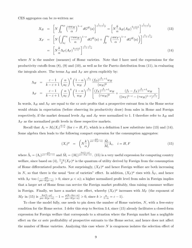
CES aggregates can be re-written as:

XH =[N

∫ aD

0

(awHα

)1−εdGH(a)

] 1ε−1

11−µ

=[Nk

αΛH(AH)

k−ε+1ε−1

] 1ε−1

11−µ

(13)

XF =[N

(∫ aX

aI

(τawHα

)1−εdGH(a) +

∫ aI

0

(awFα

)1−εdGH(a)

)] 1ε−1

11−µ

=[Nk

αΛF (AF )

k−ε+1ε−1

] 1ε−1

11−µ

(14)

where N is the number (measure) of Home varieties. Note that I have used the expressions for the

productivity cutoffs from (8), (9) and (10), as well as for the Pareto distribution from (11), in evaluating

the integrals above. The terms ΛH and ΛF are given explicitly by:

ΛH =ε− 1

k − ε+ 1

(α

aU

)k (1− αwH

) kε−1 (fD)

k1−ε+1wH

(wH)k

ΛF =ε− 1

k − ε+ 1

(α

aU

)k (1− αwH

) kε−1

[(fX)

k1−ε+1wH

(τwH)k+

(fI − fX)k

1−ε+1wH

((wF )1−ε − (τwH)1−ε)k

1−ε

]

In words, ΛH and ΛF are equal to the ex ante profits that a prospective entrant firm in the Home sector

would obtain in expectation (before observing its productivity draw) from sales in Home and Foreign

respectively, if the market demand levels AH and AF were normalized to 1. I therefore refer to ΛH and

ΛF as the normalized profit levels in these respective markets.

Recall that Ai = Mi(Xi)µ−α1−α (for i = H,F ), which is a definition I now substitute into (13) and (14).

Some algebra then leads to the following compact expression for the consumption aggregates:

(Xi)µ =(Nk

α

) µαµα−k(µ−α) Mi

MiΛi, i = H,F (15)

where Λi = (Λi)µα

µα−k(µ−α) and Mi = (Mi)kα(1−µ)

µα−k(µ−α) . (15) is a very useful expression for computing country

welfare, since based on (4), 1−µµ (XF )µ is the quantum of utility derived by Foreign from the consumption

of Home differentiated products. Not surprisingly, (XF )µ and hence Foreign welfare are both increasing

in N , so that there is the usual “love of varieties” effect. In addition, (XF )µ rises with ΛF , and hence

with ΛF too ( µαµα−k(µ−α) > 0, since µ < α); a higher normalized profit level from sales in Foreign implies

that a larger set of Home firms can service the Foreign market profitably, thus raising consumer welfare

in Foreign. Finally, we have a market size effect, whereby (XF )µ increases with MF (the exponent of

MF in (15) is kα(1−µ)µα−k(µ−α) − 1 = µ(k−kα−α)

µα−k(µ−α) > 0, since k > α1−α = ε− 1).

To close the model fully, one needs to pin down the number of Home varieties, N , with a free-entry

condition for the Home sector. I defer this step to Section 3.4, since (15) already facilitates a closed-form

expression for Foreign welfare that corresponds to a situation where the Foreign market has a negligible

effect on the ex ante profitability of prospective entrants to the Home sector, and hence does not affect

the number of Home varieties. Analyzing this case where N is exogenous isolates the selection effect of

9

FDI subsidies, by focusing attention on the set of existing Home firms that switch their mode of servicing

Foreign from exports to FDI. It will turn out later in the endogenous N case that the additional varieties

effect reinforces this selection effect, so that the welfare implications are qualitatively identical. I therefore

turn first to the analysis when the number of Home varieties is fixed.

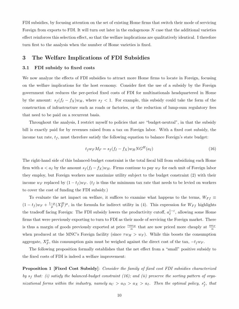
3 The Welfare Implications of FDI Subsidies

3.1 FDI subsidy to fixed costs

We now analyze the effects of FDI subsidies to attract more Home firms to locate in Foreign, focusing

on the welfare implications for the host economy. Consider first the use of a subsidy by the Foreign

government that reduces the per-period fixed costs of FDI for multinationals headquartered in Home

by the amount: sf (fI − fX)wH , where sf < 1. For example, this subsidy could take the form of the

construction of infrastructure such as roads or factories, or the reduction of lump-sum regulatory fees

that need to be paid on a recurrent basis.

Throughout the analysis, I restrict myself to policies that are “budget-neutral”, in that the subsidy

bill is exactly paid for by revenues raised from a tax on Foreign labor. With a fixed cost subsidy, the

income tax rate, tf , must therefore satisfy the following equation to balance Foreign’s state budget:

tfwFMF = sf (fI − fX)wHNGH(aI) (16)

The right-hand side of this balanced-budget constraint is the total fiscal bill from subsidizing each Home

firm with a < aI by the amount sf (fI − fX)wH . Firms continue to pay wF for each unit of Foreign labor

they employ, but Foreign workers now maximize utility subject to the budget constraint (2) with their

income wF replaced by (1− tf )wF . (tf is thus the minimum tax rate that needs to be levied on workers

to cover the cost of funding the FDI subsidy.)

To evaluate the net impact on welfare, it suffices to examine what happens to the terms, WFf ≡

(1 − tf )wF + 1−µµ (XH

F )µ, in the formula for indirect utility in (4). This expression for WFf highlights

the tradeoff facing Foreign: The FDI subsidy lowers the productivity cutoff, a1−εI , allowing some Home

firms that were previously exporting to turn to FDI as their mode of servicing the Foreign market. There

is thus a margin of goods previously exported at price τawHα that are now priced more cheaply at awF

α

when produced at the MNC’s Foreign facility (since τwH > wF ). While this boosts the consumption

aggregate, XµF , this consumption gain must be weighed against the direct cost of the tax, −tfwF .

The following proposition formally establishes that the net effect from a “small” positive subsidy to

the fixed costs of FDI is indeed a welfare improvement:

Proposition 1 [Fixed Cost Subsidy]: Consider the family of fixed cost FDI subsidies characterized

by sf that: (i) satisfy the balanced-budget constraint (16); and (ii) preserve the sorting pattern of orga-

nizational forms within the industry, namely aU > aD > aX > aI . Then the optimal policy, s∗f , that

10

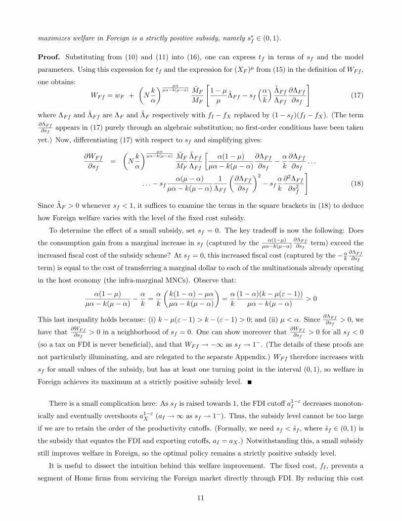
maximizes welfare in Foreign is a strictly positive subsidy, namely s∗f ∈ (0, 1).

Proof. Substituting from (10) and (11) into (16), one can express tf in terms of sf and the model

parameters. Using this expression for tf and the expression for (XF )µ from (15) in the definition of WFf ,

one obtains:

WFf = wF +(Nk

α

) µαµα−k(µ−α) MF

MF

[1− µµ

ΛFf − sf(αk

) ΛFfΛFf

∂ΛFf∂sf

](17)

where ΛFf and ΛFf are ΛF and ΛF respectively with fI − fX replaced by (1− sf )(fI − fX). (The term∂ΛFf∂sf

appears in (17) purely through an algebraic substitution; no first-order conditions have been taken

yet.) Now, differentiating (17) with respect to sf and simplifying gives:

∂WFf

∂sf=

(Nk

α

) µαµα−k(µ−α) MF

MF

ΛFfΛFf

[α(1− µ)

µα− k(µ− α)∂ΛFf∂sf

− α

k

∂ΛFf∂sf

. . .

. . .− sfα(µ− α)

µα− k(µ− α)1

ΛFf

(∂ΛFf∂sf

)2

− sfα

k

∂2ΛFf∂s2

f

](18)

Since ΛF > 0 whenever sf < 1, it suffices to examine the terms in the square brackets in (18) to deduce

how Foreign welfare varies with the level of the fixed cost subsidy.

To determine the effect of a small subsidy, set sf = 0. The key tradeoff is now the following: Does

the consumption gain from a marginal increase in sf (captured by the α(1−µ)µα−k(µ−α)

∂ΛFf∂sf

term) exceed the

increased fiscal cost of the subsidy scheme? At sf = 0, this increased fiscal cost (captured by the −αk∂ΛFf∂sf

term) is equal to the cost of transferring a marginal dollar to each of the multinationals already operating

in the host economy (the infra-marginal MNCs). Observe that:

α(1− µ)µα− k(µ− α)

− α

k=α

k

(k(1− α)− µαµα− k(µ− α)

)=α

k

(1− α)(k − µ(ε− 1))µα− k(µ− α)

> 0

This last inequality holds because: (i) k−µ(ε− 1) > k− (ε− 1) > 0; and (ii) µ < α. Since ∂ΛFf∂sf

> 0, we

have that ∂WFf

∂sf> 0 in a neighborhood of sf = 0. One can show moreover that ∂WFf

∂sf> 0 for all sf < 0

(so a tax on FDI is never beneficial), and that WFf → −∞ as sf → 1−. (The details of these proofs are

not particularly illuminating, and are relegated to the separate Appendix.) WFf therefore increases with

sf for small values of the subsidy, but has at least one turning point in the interval (0, 1), so welfare in

Foreign achieves its maximum at a strictly positive subsidy level.

There is a small complication here: As sf is raised towards 1, the FDI cutoff a1−εI decreases monoton-

ically and eventually overshoots a1−εX (aI →∞ as sf → 1−). Thus, the subsidy level cannot be too large

if we are to retain the order of the productivity cutoffs. (Formally, we need sf < sf , where sf ∈ (0, 1) is

the subsidy that equates the FDI and exporting cutoffs, aI = aX .) Notwithstanding this, a small subsidy

still improves welfare in Foreign, so the optimal policy remains a strictly positive subsidy level.

It is useful to dissect the intuition behind this welfare improvement. The fixed cost, fI , prevents a

segment of Home firms from servicing the Foreign market directly through FDI. By reducing this cost

11

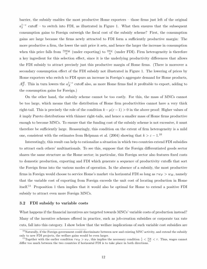
barrier, the subsidy enables the most productive Home exporters – those firms just left of the original

a1−εI cutoff – to switch into FDI, as illustrated in Figure 1. What then ensures that the subsequent

consumption gains to Foreign outweigh the fiscal cost of the subsidy scheme? First, the consumption

gains are large because the firms newly attracted to FDI form a sufficiently productive margin: The

more productive a firm, the lower the unit price it sets, and hence the larger the increase in consumption

when this price falls from τawHα (under exporting) to awF

α (under FDI). Firm heterogeneity is therefore

a key ingredient for this selection effect, since it is the underlying productivity differences that allows

the FDI subsidy to attract precisely just this productive margin of Home firms. (There is moreover a

secondary consumption effect of the FDI subsidy not illustrated in Figure 1. The lowering of prices by

Home exporters who switch to FDI spurs an increase in Foreign’s aggregate demand for Home products,

AHF . This in turn lowers the a1−εX cutoff also, as more Home firms find it profitable to export, adding to

the consumption gains for Foreign.)

On the other hand, the subsidy scheme cannot be too costly. For this, the mass of MNCs cannot

be too large, which means that the distribution of Home firm productivities cannot have a very thick

right-tail. This is precisely the role of the condition k−µ(ε− 1) > 0 in the above proof: Higher values of

k imply Pareto distributions with thinner right-tails, and hence a smaller mass of Home firms productive

enough to become MNCs. To ensure that the funding cost of the subsidy scheme is not excessive, k must

therefore be sufficiently large. Reassuringly, this condition on the extent of firm heterogeneity is a mild

one, consistent with the estimates from Helpman et al. (2004) showing that k > ε− 1.10

Interestingly, this result can help to rationalize a situation in which two countries extend FDI subsidies

to attract each others’ multinationals. To see this, suppose that the Foreign differentiated goods sector

shares the same structure as the Home sector; in particular, this Foreign sector also features fixed costs

to domestic production, exporting and FDI which generate a sequence of productivity cutoffs that sort

the Foreign firms into the various modes of operation. In the absence of a subsidy, the most productive

firms in Foreign would choose to service Home’s market via horizontal FDI so long as τwF > wH , namely

that the variable cost of exporting from Foreign exceeds the unit cost of locating production in Home

itself.11 Proposition 1 then implies that it would also be optimal for Home to extend a positive FDI

subsidy to attract even more Foreign MNCs.

3.2 FDI subsidy to variable costs

What happens if the financial incentives are targeted towards MNCs’ variable costs of production instead?

Many of the incentive schemes offered in practice, such as job-creation subsidies or corporate tax rate

cuts, fall into this category. I show below that the welfare implications of such variable cost subsidies are10Naturally, if the Foreign government could discriminate between new and existing MNC activity, and extend the subsidy

only to new FDI projects, the welfare gains would be even larger.11Together with the earlier condition τwH > wF , this implies the necessary condition 1

τ< wH

wF< τ . Thus, wages cannot

differ too much between the two countries if horizontal FDI is to take place in both directions.

12

similar to what we have seen for a fixed cost subsidy.

Consider a subsidy to the variable costs of Home MNCs’ production in Foreign that reduces their

effective unit wage costs from wF to (1− sv)wF , where sv < 1. As before, suppose that these subsidies

are financed by levying a tax, tv, on each worker. If this scheme is to be budget-neutral, then:

tvwFMF = svwFNAF

((1− sv)wF

α

)−εV H(aI) (19)

where the right-hand side of (19) is the total amount paid out as production subsidies to the multi-

nationals. Note that a higher demand for Home final goods, AF , will now raise the total subsidy bill

directly under a variable cost subsidy scheme. We have the following parallel result concerning the welfare

improvement from a subsidy to MNCs’ variable costs of production:

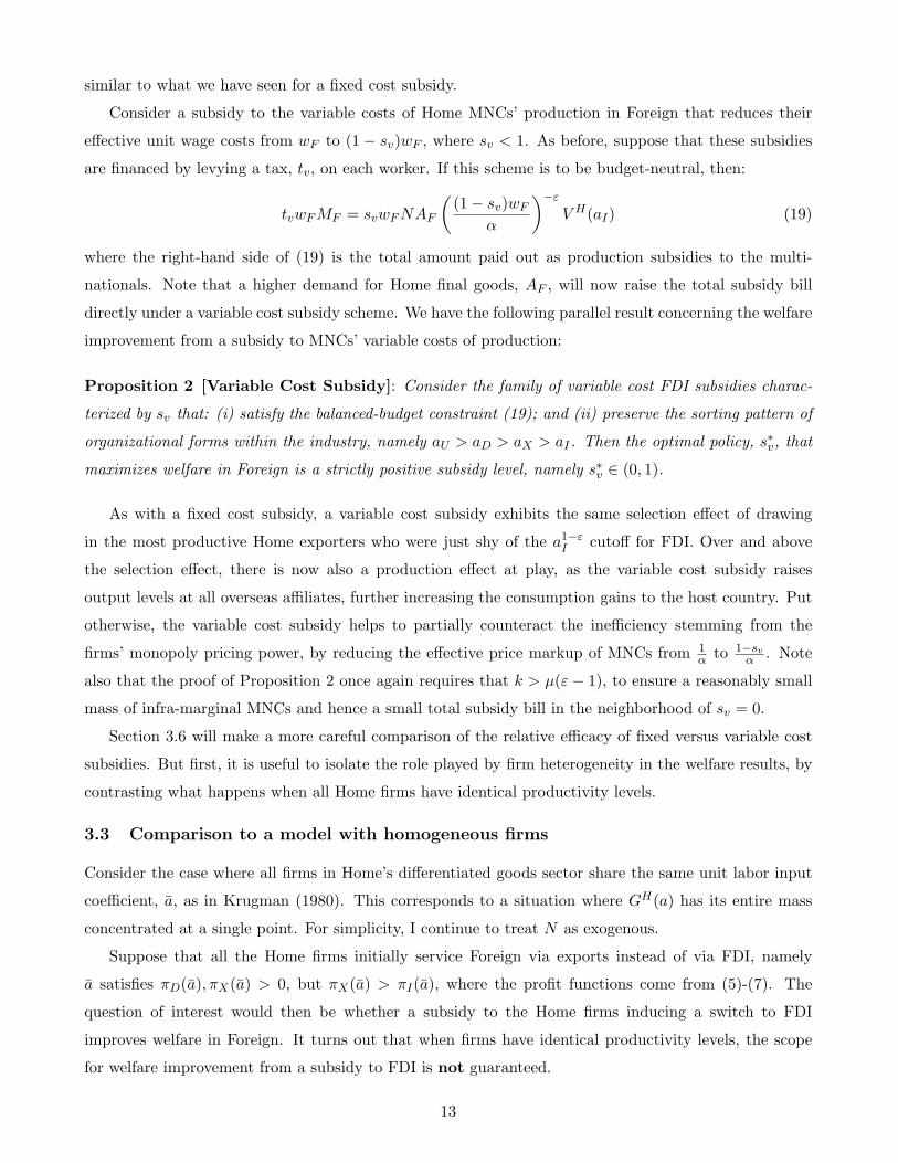
Proposition 2 [Variable Cost Subsidy]: Consider the family of variable cost FDI subsidies charac-

terized by sv that: (i) satisfy the balanced-budget constraint (19); and (ii) preserve the sorting pattern of

organizational forms within the industry, namely aU > aD > aX > aI . Then the optimal policy, s∗v, that

maximizes welfare in Foreign is a strictly positive subsidy level, namely s∗v ∈ (0, 1).

As with a fixed cost subsidy, a variable cost subsidy exhibits the same selection effect of drawing

in the most productive Home exporters who were just shy of the a1−εI cutoff for FDI. Over and above

the selection effect, there is now also a production effect at play, as the variable cost subsidy raises

output levels at all overseas affiliates, further increasing the consumption gains to the host country. Put

otherwise, the variable cost subsidy helps to partially counteract the inefficiency stemming from the

firms’ monopoly pricing power, by reducing the effective price markup of MNCs from 1α to 1−sv

α . Note

also that the proof of Proposition 2 once again requires that k > µ(ε− 1), to ensure a reasonably small

mass of infra-marginal MNCs and hence a small total subsidy bill in the neighborhood of sv = 0.

Section 3.6 will make a more careful comparison of the relative efficacy of fixed versus variable cost

subsidies. But first, it is useful to isolate the role played by firm heterogeneity in the welfare results, by

contrasting what happens when all Home firms have identical productivity levels.

3.3 Comparison to a model with homogeneous firms

Consider the case where all firms in Home’s differentiated goods sector share the same unit labor input

coefficient, a, as in Krugman (1980). This corresponds to a situation where GH(a) has its entire mass

concentrated at a single point. For simplicity, I continue to treat N as exogenous.

Suppose that all the Home firms initially service Foreign via exports instead of via FDI, namely

a satisfies πD(a), πX(a) > 0, but πX(a) > πI(a), where the profit functions come from (5)-(7). The

question of interest would then be whether a subsidy to the Home firms inducing a switch to FDI

improves welfare in Foreign. It turns out that when firms have identical productivity levels, the scope

for welfare improvement from a subsidy to FDI is not guaranteed.

13

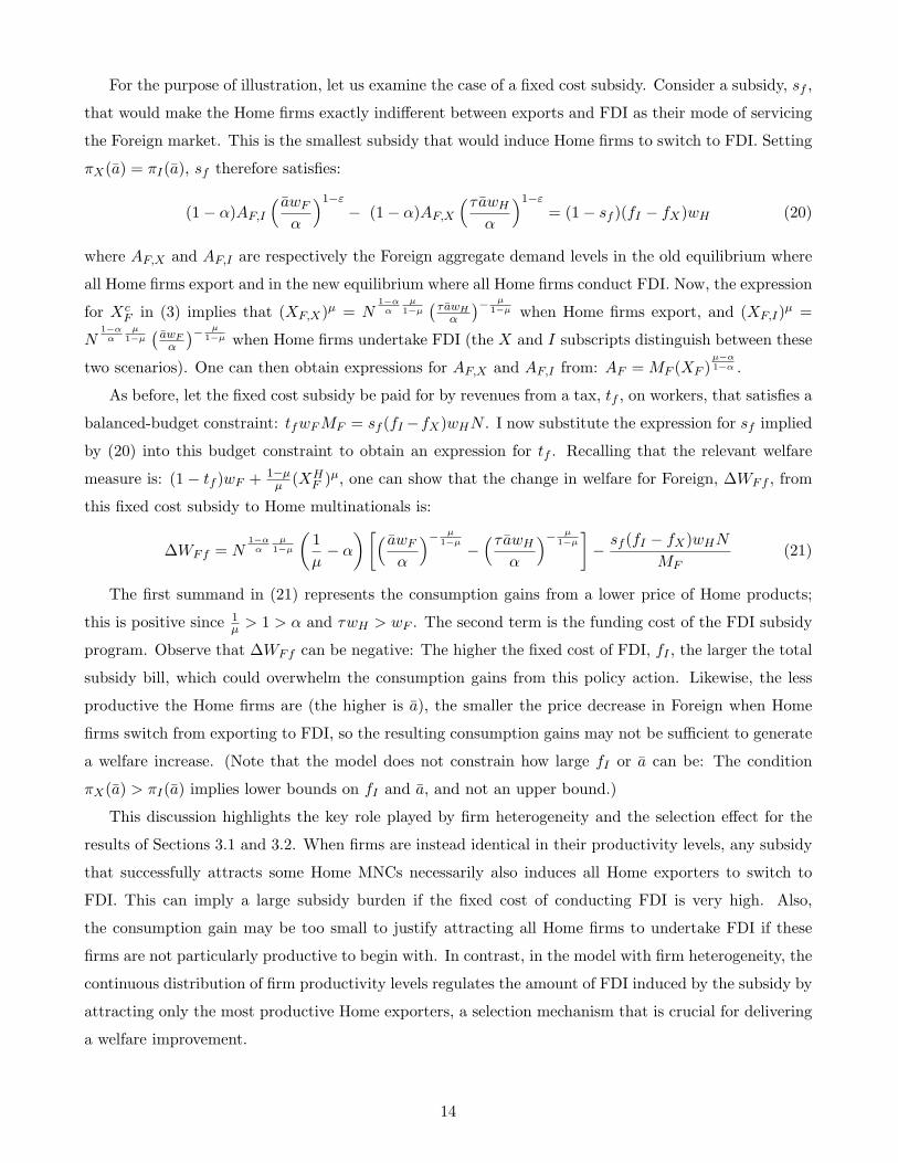
For the purpose of illustration, let us examine the case of a fixed cost subsidy. Consider a subsidy, sf ,

that would make the Home firms exactly indifferent between exports and FDI as their mode of servicing

the Foreign market. This is the smallest subsidy that would induce Home firms to switch to FDI. Setting

πX(a) = πI(a), sf therefore satisfies:

(1− α)AF,I( awF

α

)1−ε− (1− α)AF,X

(τ awHα

)1−ε= (1− sf )(fI − fX)wH (20)

where AF,X and AF,I are respectively the Foreign aggregate demand levels in the old equilibrium where

all Home firms export and in the new equilibrium where all Home firms conduct FDI. Now, the expression

for XcF in (3) implies that (XF,X)µ = N

1−αα

µ1−µ

(τ awHα

)− µ1−µ when Home firms export, and (XF,I)µ =

N1−αα

µ1−µ

(awFα

)− µ1−µ when Home firms undertake FDI (the X and I subscripts distinguish between these

two scenarios). One can then obtain expressions for AF,X and AF,I from: AF = MF (XF )µ−α1−α .

As before, let the fixed cost subsidy be paid for by revenues from a tax, tf , on workers, that satisfies a

balanced-budget constraint: tfwFMF = sf (fI−fX)wHN . I now substitute the expression for sf implied

by (20) into this budget constraint to obtain an expression for tf . Recalling that the relevant welfare

measure is: (1− tf )wF + 1−µµ (XH

F )µ, one can show that the change in welfare for Foreign, ∆WFf , from

this fixed cost subsidy to Home multinationals is:

∆WFf = N1−αα

µ1−µ

(1µ− α

)[( awFα

)− µ1−µ −

(τ awHα

)− µ1−µ]−sf (fI − fX)wHN

MF(21)

The first summand in (21) represents the consumption gains from a lower price of Home products;

this is positive since 1µ > 1 > α and τwH > wF . The second term is the funding cost of the FDI subsidy

program. Observe that ∆WFf can be negative: The higher the fixed cost of FDI, fI , the larger the total

subsidy bill, which could overwhelm the consumption gains from this policy action. Likewise, the less

productive the Home firms are (the higher is a), the smaller the price decrease in Foreign when Home

firms switch from exporting to FDI, so the resulting consumption gains may not be sufficient to generate

a welfare increase. (Note that the model does not constrain how large fI or a can be: The condition

πX(a) > πI(a) implies lower bounds on fI and a, and not an upper bound.)

This discussion highlights the key role played by firm heterogeneity and the selection effect for the

results of Sections 3.1 and 3.2. When firms are instead identical in their productivity levels, any subsidy

that successfully attracts some Home MNCs necessarily also induces all Home exporters to switch to

FDI. This can imply a large subsidy burden if the fixed cost of conducting FDI is very high. Also,

the consumption gain may be too small to justify attracting all Home firms to undertake FDI if these

firms are not particularly productive to begin with. In contrast, in the model with firm heterogeneity, the

continuous distribution of firm productivity levels regulates the amount of FDI induced by the subsidy by

attracting only the most productive Home exporters, a selection mechanism that is crucial for delivering

a welfare improvement.

14

3.4 Endogenizing the number of varieties

To this point, the number of Home varieties, N , has been treated as exogenous in order to focus on the

shift in the FDI cutoff, a1−εI , that a FDI subsidy induces. However, the subsidy also increases the ex ante

profitability of potential entrants to the Home differentiated goods sector, particularly when the host

country is a big market. I endogenize N in this subsection to solve for the full industry equilibrium. The

model remains highly tractable, with the subsequent increase in the number of Home varieties reinforcing

the gains that accrue to Foreign consumers.

Free-entry: N is pinned down by a free-entry condition, which closes the industry equilibrium in

Section 2. Potential entrants do not observe their productivity draw 1/a until after they have started

paying a per-period fixed cost of entry equal to fE units of Home labor. These prospective firms weigh

their expected profits against this fixed cost, with zero ex ante profits prevailing in equilibrium. This

free-entry condition is:

fEwH = (1− α)AH(wHα

)1−εV H(aD) + (1− α)AF

(τwHα

)1−ε(V H(aX)− V H(aI)) . . .

. . .+ (1− α)AF(wFα

)1−εV H(aI)− fDwHGH(aD) . . .

. . .− fXwH(GH(aX)−GH(aI))− fIwHGH(aI) (22)

= ΛH(AH)kε−1 + ΛF (AF )

kε−1 (23)

where the right-hand side of (22) comes from integrating over the productivity distribution, GH(a), to

compute expected profits prior to entry. The compact expression in (23) comes from a further substitution

and simplification, using the productivity cutoffs in (8)-(10) and the Pareto distribution expressions in

(11)-(12). Equation (23) has an intuitive interpretation: ΛH(AH)kε−1 captures the normalized profits

from sales in Home weighted by a measure of the demand level in the Home market, with ΛF (AF )kε−1

being the analogous term for the Foreign market. The free-entry condition thus equates the fixed cost of

entry with the sum of expected profits from both markets.

Substituting now from (13) and (14) into the definition: Ai = Mi(Xi)µ−α1−α , yields:

(Ai)kε−1 =

(Nk

α

) k(µ−α)µα−k(µ−α) Λi

ΛiMi , i = H,F (24)

The aggregate demand level in market i facing each firm is thus increasing in the size of that market,

Mi, while decreasing in the number of competing varieties, N (since µ < α).

The free-entry condition (23) and the two equations in (24) comprise a system of three equations in

three unknowns, N , AH and AF , that can be solved for the equilibrium in the Home sector. Substituting

from (24) into (23) and re-arranging yields:

N =α

k

[MHΛH + MF ΛF

fEwH

]µα−k(µ−α)k(α−µ)

(25)

15

Not surprisingly, an increase in entry costs, fE , decreases the number of Home varieties. Similarly, a rise

in Home wages, wH , decreases expected normalized profits (both ΛH and ΛF ), while also raising entry

costs, fEwH , and hence reduces N . This expression for N can be substituted into (15) to solve for the

consumption aggregate (XF )µ, and hence welfare, as a function of model parameters only. Note that

both N and (XF )µ exhibit similar comparative statics, with both variables rising as the market size, Mi,

or normalized profit levels, Λi, in either country increases.

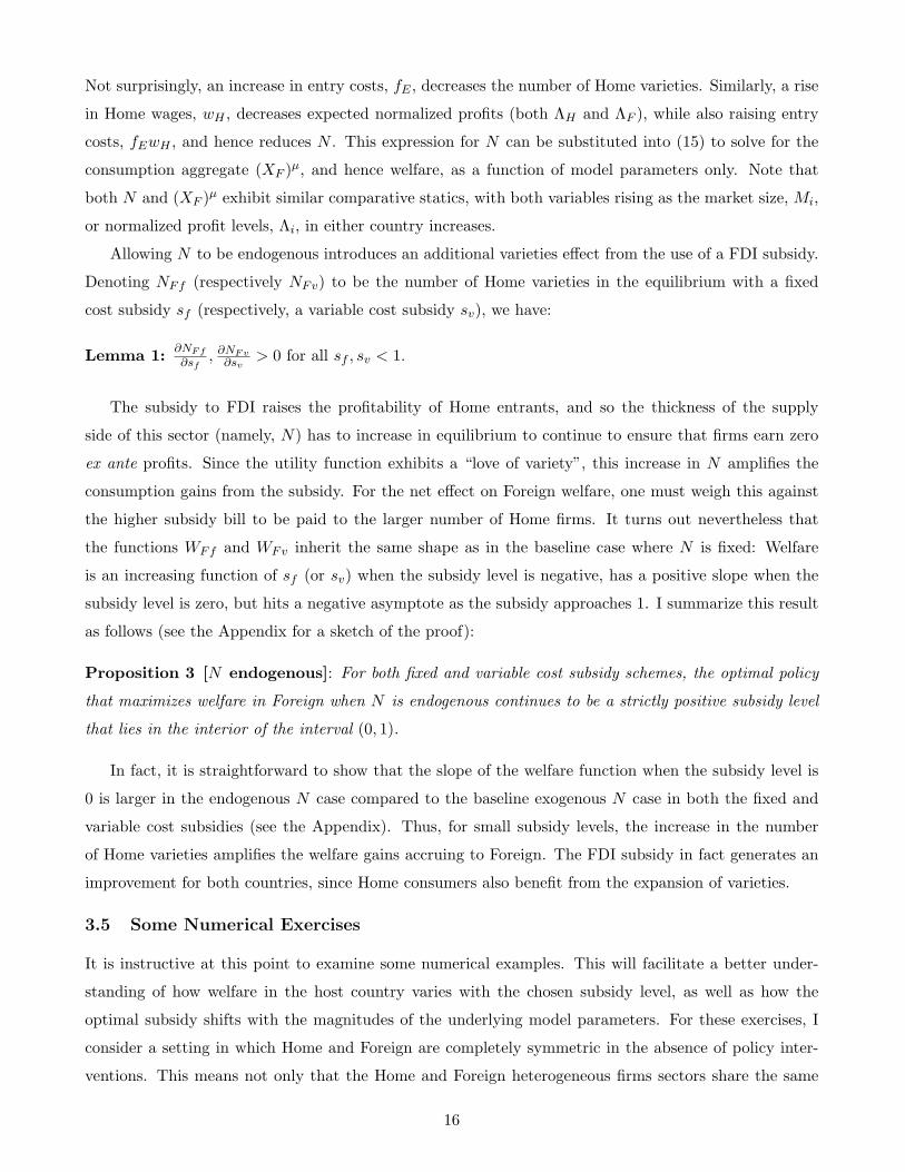
Allowing N to be endogenous introduces an additional varieties effect from the use of a FDI subsidy.

Denoting NFf (respectively NFv) to be the number of Home varieties in the equilibrium with a fixed

cost subsidy sf (respectively, a variable cost subsidy sv), we have:

Lemma 1: ∂NFf∂sf

, ∂NFv∂sv> 0 for all sf , sv < 1.

The subsidy to FDI raises the profitability of Home entrants, and so the thickness of the supply

side of this sector (namely, N) has to increase in equilibrium to continue to ensure that firms earn zero

ex ante profits. Since the utility function exhibits a “love of variety”, this increase in N amplifies the

consumption gains from the subsidy. For the net effect on Foreign welfare, one must weigh this against

the higher subsidy bill to be paid to the larger number of Home firms. It turns out nevertheless that

the functions WFf and WFv inherit the same shape as in the baseline case where N is fixed: Welfare

is an increasing function of sf (or sv) when the subsidy level is negative, has a positive slope when the

subsidy level is zero, but hits a negative asymptote as the subsidy approaches 1. I summarize this result

as follows (see the Appendix for a sketch of the proof):

Proposition 3 [N endogenous]: For both fixed and variable cost subsidy schemes, the optimal policy

that maximizes welfare in Foreign when N is endogenous continues to be a strictly positive subsidy level

that lies in the interior of the interval (0, 1).

In fact, it is straightforward to show that the slope of the welfare function when the subsidy level is

0 is larger in the endogenous N case compared to the baseline exogenous N case in both the fixed and

variable cost subsidies (see the Appendix). Thus, for small subsidy levels, the increase in the number

of Home varieties amplifies the welfare gains accruing to Foreign. The FDI subsidy in fact generates an

improvement for both countries, since Home consumers also benefit from the expansion of varieties.

3.5 Some Numerical Exercises

It is instructive at this point to examine some numerical examples. This will facilitate a better under-

standing of how welfare in the host country varies with the chosen subsidy level, as well as how the

optimal subsidy shifts with the magnitudes of the underlying model parameters. For these exercises, I

consider a setting in which Home and Foreign are completely symmetric in the absence of policy inter-

ventions. This means not only that the Home and Foreign heterogeneous firms sectors share the same

16

structure, but additionally that the two sectors share identical parameter values, including the Pareto

shape parameter, k, and the industry cost parameters.12 (For the analytical results derived previously

in Sections 3.1-3.4, I only require that the Home and Foreign sectors share the same structure, but do

not need to assume that they share identical parameter values.)

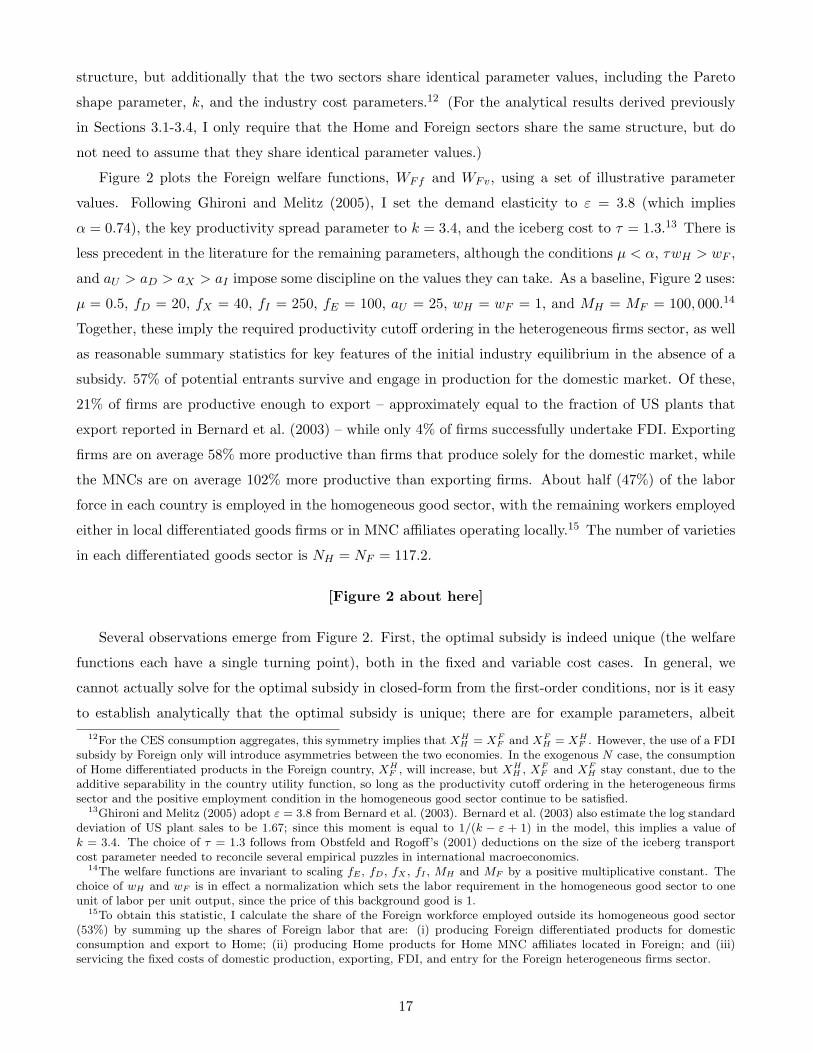
Figure 2 plots the Foreign welfare functions, WFf and WFv, using a set of illustrative parameter

values. Following Ghironi and Melitz (2005), I set the demand elasticity to ε = 3.8 (which implies

α = 0.74), the key productivity spread parameter to k = 3.4, and the iceberg cost to τ = 1.3.13 There is

less precedent in the literature for the remaining parameters, although the conditions µ < α, τwH > wF ,

and aU > aD > aX > aI impose some discipline on the values they can take. As a baseline, Figure 2 uses:

µ = 0.5, fD = 20, fX = 40, fI = 250, fE = 100, aU = 25, wH = wF = 1, and MH = MF = 100, 000.14

Together, these imply the required productivity cutoff ordering in the heterogeneous firms sector, as well

as reasonable summary statistics for key features of the initial industry equilibrium in the absence of a

subsidy. 57% of potential entrants survive and engage in production for the domestic market. Of these,

21% of firms are productive enough to export – approximately equal to the fraction of US plants that

export reported in Bernard et al. (2003) – while only 4% of firms successfully undertake FDI. Exporting

firms are on average 58% more productive than firms that produce solely for the domestic market, while

the MNCs are on average 102% more productive than exporting firms. About half (47%) of the labor

force in each country is employed in the homogeneous good sector, with the remaining workers employed

either in local differentiated goods firms or in MNC affiliates operating locally.15 The number of varieties

in each differentiated goods sector is NH = NF = 117.2.

[Figure 2 about here]

Several observations emerge from Figure 2. First, the optimal subsidy is indeed unique (the welfare

functions each have a single turning point), both in the fixed and variable cost cases. In general, we

cannot actually solve for the optimal subsidy in closed-form from the first-order conditions, nor is it easy

to establish analytically that the optimal subsidy is unique; there are for example parameters, albeit12For the CES consumption aggregates, this symmetry implies that XH

H = XFF and XF

H = XHF . However, the use of a FDI

subsidy by Foreign only will introduce asymmetries between the two economies. In the exogenous N case, the consumptionof Home differentiated products in the Foreign country, XH

F , will increase, but XHH , XF

F and XFH stay constant, due to the

additive separability in the country utility function, so long as the productivity cutoff ordering in the heterogeneous firmssector and the positive employment condition in the homogeneous good sector continue to be satisfied.

13Ghironi and Melitz (2005) adopt ε = 3.8 from Bernard et al. (2003). Bernard et al. (2003) also estimate the log standarddeviation of US plant sales to be 1.67; since this moment is equal to 1/(k − ε + 1) in the model, this implies a value ofk = 3.4. The choice of τ = 1.3 follows from Obstfeld and Rogoff’s (2001) deductions on the size of the iceberg transportcost parameter needed to reconcile several empirical puzzles in international macroeconomics.

14The welfare functions are invariant to scaling fE , fD, fX , fI , MH and MF by a positive multiplicative constant. Thechoice of wH and wF is in effect a normalization which sets the labor requirement in the homogeneous good sector to oneunit of labor per unit output, since the price of this background good is 1.

15To obtain this statistic, I calculate the share of the Foreign workforce employed outside its homogeneous good sector(53%) by summing up the shares of Foreign labor that are: (i) producing Foreign differentiated products for domesticconsumption and export to Home; (ii) producing Home products for Home MNC affiliates located in Foreign; and (iii)servicing the fixed costs of domestic production, exporting, FDI, and entry for the Foreign heterogeneous firms sector.

17

very extreme ones, for which the welfare functions are not globally concave.16 For all practical purposes

though, WFf and WFv do exhibit a unique maximum for a wide range of parameter values. (For a

more formal treatment, the Appendix derives a sufficient condition for the uniqueness of the optimal

fixed cost subsidy in the exogenous N case: 2(ε− 1) > k, which is satisfied by our baseline parameters.)

Second, allowing the number of varieties, N , to respond to the subsidy accentuates the welfare functions

without altering their general shape, as was asserted in Proposition 3. For the positive subsidy levels in

Figure 2, the case with N endogenous (dashed-line graphs) has welfare levels raised above that where

N is held fixed (solid-line graphs).17 Note that while there are other parameter configurations that also

respect the key structural assumptions of the model, namely that in both countries: (i) some labor be

employed in the background sector, and (ii) the desired ordering of the productivity cutoffs be preserved

(aU > aD > aX > aI), the shape of the welfare functions and the qualitative features of the equilibria

are nevertheless very similar under these alternative parameterizations. I have moreover checked that

these two structural assumptions hold over the range of subsidy values plotted for each welfare function

in Figure 2, and in particular at the optimal subsidy.18

Figure 3 explores some comparative statics of the optimal subsidy. I graph these for the case of a

variable cost subsidy; the behavior of the optimal fixed cost subsidy against each parameter is similar,

but quantitatively smaller. I examine first the effect of adjusting the parameters that relate to the cost

of exporting, namely τ and fX . Ceteris paribus, as τ is raised from 1.05 to 1.4 in panel A, the share

of exporting firms decreases steadily from 43% to 14%, similar to the range for this summary statistic

(15%-45%) considered in Costantini and Melitz (2007). Likewise, in panel B, as fX is increased from 20

to 55 units of labor, the share of exporting firms decreases from 50% to 13%. Both panels show that

a larger exporting cost is associated with a higher optimal subsidy. Intuitively, the larger the barriers

faced by exporters, the greater the gains to the host country from attracting firms to switch into FDI,

and hence the higher the optimal subsidy. Conversely, a higher fixed cost of FDI, fI , lowers the optimal

subsidy (panel C), since a given FDI subsidy will be less effective at inducing firms to go multinational

when fI is high. The optimal subsidy is not particularly sensitive to the fixed cost of domestic production

fD (panel D), since the FDI subsidy affects a margin of firms that is much more productive than those

that produce solely for the domestic market. In fact, in the exogenous N case, fD does not alter the

optimal subsidy at all (fD does not appear in the first-order conditions that pin down s∗F or s∗v).

Panel E focuses on the Pareto shape parameter k. There is an interplay between two effects as

k increases: As less mass is placed on the right-tail of the productivity distribution, fewer firms can

potentially become multinationals, which reduces both the consumption gain and the total subsidy bill16When k is large (for example, k = 25) and µ is raised closer to the value of α (for example, µ = 0.6 and α = 0.74), WFv

ceases to be globally concave in the interval (0, 1).17For the exogenous N graphs, the value of N used is given by (25) with the subsidy level set to 0.18In Figure 2, it takes a large subsidy (sf = 0.79 or sv = 0.32 respectively) to lower the FDI cutoff, a1−ε

I , down tothe exporting cutoff, a1−ε

X . The welfare functions reach their turning points before these respective upper bounds on thepermissible subsidy level, ensuring that aX > aI at the optimal subsidy.

18

from a given FDI subsidy. The reduced consumption gain tends to lower the optimal subsidy, whereas

the smaller fiscal cost tends to raise the optimal subsidy instead. For the exogenous N case, the latter

effect is more salient for smaller values of k. However, the former effect dominates as k increases, and

the optimal subsidy appears to asymptote towards zero. This is consistent with the idea that as we

approach the Krugman (1980) case with homogeneous firms (k → ∞), the scope for a FDI subsidy to

generate a welfare gain becomes more limited. There is a caveat here, namely that as k increases, the

productivity distribution becomes more concentrated at a point mass. In particular, the domestic cutoff

aD increases and eventually overshoots aU , so that the condition aU > aD can no longer be satisfied.

What is plotted as the optimal subsidy in panel E is the value of sv at which the welfare function

WFv reaches its maximum, but one should bear in mind that one cannot increase k indefinitely without

violating the required ordering of productivity cutoffs in the industry equilibrium.19

[Figure 3 about here]

Last but not least, an increase in the demand elasticity, ε, lowers the optimal subsidy (panel F).

The consumption gains from a FDI subsidy are intuitively smaller if there is more scope for substitution

between differentiated products.20 Finally, note that throughout Figure 3, the optimal subsidy when N

is endogenous (solid-line graphs) exceeds that when N is exogenous (dashed-line graphs). This is not

surprising since the host country stands to gain more when the number of Home varieties is allowed to

increase in response to the subsidy (Proposition 3).

3.6 Fixed versus Variable Cost Subsidies

How does the welfare level at the optimal fixed cost subsidy, s∗f , compare to that at the optimal variable

cost subsidy, s∗v? Figure 2 points to a prima facie case in favor of variable cost subsidies from the

perspective of Foreign welfare levels, since these appear to generate much larger gains than fixed cost

subsidies. As argued earlier, a variable cost subsidy delivers a greater kick to welfare by raising each

firm’s output from its inefficiently low level. This production effect is absent with a fixed cost subsidy,

which only affects a Home firm’s decision on exporting versus FDI.

Formally, we can derive the following result to compare the efficacy of the two types of subsidy

schemes (see the Appendix for a proof):

Proposition 4 [Fixed versus variable cost subsidy]: Suppose that ε > 2 and that the number of

Home varieties is fixed. Consider only those subsidies with sf , sv ∈ (0, 1) that: (i) satisfy a balanced-

budget constraint; and (ii) preserve the sorting pattern of organizational forms within the industry, namely19I do not encounter this problem with the other model parameters. For the range over which the other parameters are

graphed in Figure 3, the productivity ordering in the heterogeneous firms sector and the positive employment condition forthe homogeneous good sector are satisfied in both countries.

20As I vary ε in panel F, I have held the log standard deviation of plant sales constant at 1.67 (from Bernard et al., 2003).Since this moment is equal to 1/(k − ε + 1) in the model, this means that the value of k adjusts to keep the log standarddeviation constant. The graph looks similar if I instead fix k at its initial value of k = 3.4 as I vary ε.

19

aU > aD > aX > aI . Then, a variable cost subsidy that incurs the same total subsidy bill as a fixed cost

subsidy delivers greater consumption gains to Foreign.

A variable cost subsidy therefore has more bang for the buck, delivering a greater increase in utility

than a corresponding fixed cost subsidy with the same amount of public spending. It follows that the

welfare level achieved by the optimal variable cost subsidy, s∗v, will be higher than that reached by the

optimal fixed cost subsidy, s∗f . The requirement that ε > 2 also has an intuitive interpretation: Consumer

demand needs to be sufficiently elastic, so that a given price decrease with the introduction of a variable

cost subsidy will generate a large increase in consumption. (Note that this condition is satisfied by the

baseline parameter values used in the numerical exercises.)

It is important however to highlight a key caveat. As it stands, the only motive in the model for a

Home firm to open a plant in Foreign is to service that market, so that FDI is of a purely horizontal

nature. In practice, much of the foreign affiliate activity that takes place services more than just the

local market, with some output from the foreign assembly plant being shipped back to the home or third-

country markets (Eckholm et al., 2003, Grossman et al., 2006). The scope for welfare improvement from

a variable cost subsidy is potentially fragile to incorporating such an export-platform motive, since re-

exports represent subsidized production for which the consumption gains accrue purely to other countries.

If the third-country market that the affiliate is servicing is large, re-exports would raise the total subsidy

bill without generating corresponding gains to domestic consumers, potentially negating the scope for a

welfare improvement. To avoid this outcome, the subsidy would have to be administered as a domestic

sales or retail credit (a rebate to local consumption), instead of as a direct subsidy to production. In

contrast, this caveat does not apply to a fixed cost subsidy, since that alters only firms’ mode of servicing

the Foreign market, but does not affect firms’ choice of output levels.

4 Some Extensions

I briefly discuss two extensions. The first examines a similar policy intervention, namely import subsidies

to promote more exporting by Home firms to the Foreign market. The second explores the robustness of

the results under an alternative utility function that builds in richer income effects.

4.1 Import subsidies

The above model lends itself naturally to an analysis of trade policy. It is well-established that the

optimal policy for a country with a downward-sloping import demand curve is to levy a tariff, since the

tariff revenue outstrips the loss in consumer surplus when the tariff is small (see Helpman and Krugman,

1989). In view of this result, previous arguments advanced for the opposite policy of an import subsidy

have raised the possibility of dynamic gains. Dasgupta and Stiglitz (1988) posit that when learning-by-

doing effects are large, it may be optimal to subsidize imports to promote learning by foreign producers,

20

which lowers prices in the long run.

The framework with heterogeneous firms suggests another mechanism through which import subsidies

might be beneficial, by increasing the set of products that is exported to the Foreign market. In this case,

however, the intuition is less neat: An import subsidy will induce some Home firms to start exporting

to Foreign, delivering positive consumption gains (from a leftward shift of the a1−εX cutoff in Figure 1),

but it will also prompt some Home MNCs to switch from horizontal FDI back to exporting, raising

prices for Foreign consumers for this margin of goods (as the a1−εI cutoff shifts to the right). It is

nevertheless straightforward to analyze the welfare impact of either a fixed or variable cost subsidy to

imports, following steps analogous to Sections 3.1 and 3.2. For this alternative policy intervention, it

turns out that a small subsidy is once again welfare-improving:

Proposition 5 [Import Subsidies]: Consider the family of fixed cost (respectively variable cost) import

subsidies that: (i) satisfy a balanced-budget constraint; and (ii) preserve the sorting pattern of organiza-

tional forms within the industry, namely aU > aD > aX > aI . Then the optimal policy that maximizes

welfare in Foreign is a strictly positive subsidy level.

The proof is similar to that for Propositions 1 and 2, as it hinges on showing that the welfare function

has a positive slope in the neighborhood where the subsidy level is zero. (Details are in the supplementary

Appendix.) Thus, the consumption gains from drawing in more firms at the a1−εX cutoff outweigh the

loss of MNCs at the a1−εI margin, with the intuition being that there is a greater density of firms at the

exporting cutoff than the FDI cutoff. The proof also relies on the inequality: k > ε − 1, to ensure that

the mass of firms to be subsidized is not too large. Naturally, when N is allowed to be endogenous, the

subsequent increase in the number of varieties in the Home sector reinforces the welfare gains from a

small subsidy, akin to the varieties effect in Proposition 3.

It is useful to highlight how this result can be reconciled with Demidova and Rodriguez-Clare (2008),

who find instead that the optimal policy is an import tariff when the domestic economy is composed

solely of a heterogeneous firms sector. Their model identifies two welfare distortions, both of which are

also present in this paper. There is first a markup distortion, by which markup pricing by domestic firms

leads to an under-consumption of domestic varieties (imports are purchased at opportunity cost from

the perspective of the domestic economy). Second, there is a consumer surplus distortion, by which the

failure of Foreign consumers to internalize the effects of their purchases on the entry of Home firms leads

to an under-consumption of import varieties (which gives rise to what I term the selection effect). In

Demidova and Rodriguez-Clare (2008), it turns out that the former effect dominates the latter, so that

it is optimal to impose an import tariff to raise consumption of domestic varieties. Intuitively, in the

absence of a homogeneous good sector, the domestic wage is endogenous, so an import tariff raises the

demand for domestic varieties and hence wages. This direct boost to income turns out to be sufficient

to offset the loss due to the decrease in import varieties. This is however no longer the case when a

21

constant returns-to-scale homogeneous good sector (such as the x0i sector) is included in the model. An

import tariff would now introduce a further distortion, by increasing consumption of the homogeneous

good above its optimal level. Achieving the first-best instead requires an import subsidy together with

a consumption subsidy for domestic varieties, to correct the consumer surplus and markup distortions

respectively. In particular, an import tariff alone cannot achieve the first-best, and an import subsidy is

now welfare-improving. In sum, the divergence in results in the two papers can be traced to the distinct

production structures considered in each model.21

4.2 Robustness to specification of utility function

The quasilinear utility function (1) has facilitated the analysis by providing a closed-form expression for

country welfare. One relevant concern is that this function carries the restriction that any exogenous

change in labor income, wF , affects only the consumption level of the homogeneous good. If instead the

demand for differentiated products were also to exhibit a positive income elasticity, then the decrease in

disposable income from the labor tax could dampen the welfare gains from a FDI subsidy.

A natural way to incorporate more general income effects is with the following country i utility

function:

Ui =

(x0i )ρ +

∑c=H,F

1µ

(Xci )µ

ρµ

1ρ

, 0 < ρ < µ < α < 1

This introduces a constant elasticity of substitution (equal to 11−ρ) between the demand for the homo-

geneous good, x0i , and the differentiated varieties aggregate,

∑c=H,F

1µ(Xc

i )µ. (We require ρ < µ, so

that differentiated products are always better substitutes for each other than the homogeneous good.)

With utility no longer quasilinear in x0i , the demand for differentiated products now depends directly

on disposable income, (1 − tf )wF , as well as on the demand for varieties from the other country. Also,

the utility derived from consumption of the Home and Foreign differentiated goods will no longer be

additively separable. This more general specification does however sacrifice some tractability, as welfare

can no longer be written down in a convenient closed-form, so the subsidy analysis requires us to perform

comparative statics on the system of equations that defines the industry equilibrium.

It turns out that our welfare results continue to hold with this alternative utility function, with the

optimal policy being a small subsidy to MNCs. (The proof is in the Appendix.) Of note, the condition

k > ε− 1 once again ensures a relatively small mass of MNCs, and hence a small total funding cost for

the subsidy scheme. This further implies a small per worker tax burden, tf , so that the negative income

effect of this tax on the consumption of differentiated products fails to wipe out the overall welfare gain.

It is thus reassuring that the welfare implications for FDI subsidies carry through when some allowance

is made for the demand for differentiated products to be subject to income effects.21Demidova and Rodriguez-Clare (2008) also recognize this point, and briefly mention in their Conclusion how their results

would change if a constant returns-to-scale sector where prices are set at marginal cost were included in the model.

22

5 Conclusion

This paper builds on a growing literature on firm heterogeneity in international trade by extending it

to a policy analysis of FDI subsidies. The paper developed a two-country version of the Helpman et al.

(2004) model that admits a closed-form expression for welfare. Focusing on the consumption gains from

attracting FDI (the lowered prices at which MNCs’ products are sold in the host country), I showed

that a small subsidy to either MNCs’ fixed or variable costs of operation leads to a rise in welfare in

the FDI host country, after accounting for the cost of financing this policy through a tax on workers’

income. Of note, these consumption gains already generate a welfare improvement for the host economy,

even while putting aside other potential gains from such further considerations as technological spillovers,

agglomeration economies, or an increased demand for local labor.

This welfare improvement is driven by a selection effect, highlighting the key role played by firm

heterogeneity in these results. The FDI subsidy enables the host country to attract those Home exporters

that previously fell just shy of the FDI cutoff to switch to servicing the Foreign market via horizontal FDI.

Being from a relatively productive margin, these firms set lower prices and their products are demanded

in relatively high quantities, so the resulting savings on cross-border transport costs from the switch to

FDI delivers substantial consumption gains to Foreign. At the same time, for these consumption gains

to exceed the funding cost of the subsidy scheme, one also needs the mass of MNCs to be subsidized

to be relatively small. This translates into a requirement that the firm distribution not place too large

a mass on high productivity levels. What is particularly neat is that the implied formal condition on

the heterogeneity parameter of firm productivities is one that empirical research has shown is readily

satisfied in practice (Helpman et al. 2004). The model also concludes that in general, a variable cost

subsidy delivers a larger welfare improvement than a fixed cost subsidy: A reduction in MNCs’ variable

costs of operation has an additional production effect that partially corrects the inefficiently low output

levels stemming from firms’ monopoly pricing power.

As a cautionary concluding remark, it has to be stressed that this paper should not be read as

a carte blanche endorsement of generous subsidies to FDI. Naturally, the actual implementation and

governance of any such schemes will have to be carried out carefully, in order to determine what the

appropriate subsidy level should be. Moreover, while the model does establish sharp benchmark results,

it abstracts from such issues as strategic competition among countries for FDI or political economy forces

(the presence of lobbies) that could qualify and alter the conclusions on the efficacy of FDI subsidies.22

These are all relevant issues for future work to consider within this setting with heterogeneous firms.

22See for example Janeba (2004), where FDI subsidies generate a redistributive effect from workers to firms, which limitsthe scope for large subsidies if workers have sufficient political clout. Also, Janeba (2002) considers a model where the hostgovernment is unable to make credible long-term commitments to its announced tax or subsidy policies.

23

6 References

Aitken, B., Harrison, A., 1999. Do domestic firms benefit from direct foreign investment? Evidencefrom Venezuela. American Economic Review 89, 605-618.

Baldwin, R., Okubo, T., 2006. Heterogeneous firms, agglomeration and economic geography: Spatialselection and sorting. Journal of Economic Geography 6, 323-346.

Bernard, A., Eaton, J., Jensen, J.B., Kortum, S., 2003. Plants and productivity in international trade.American Economic Review 93, 1268-1290.

Black, D.A., Hoyt, W.H., 1989. Bidding for firms. American Economic Review 79, 1249-1256.

Costantini, J., Melitz, M.J., 2007. The Dynamics of Firm-Level Adjustment to Trade Liberalization.Forthcoming in Helpman, E., Marin, D., Verdier, T., The Organization of Firms in a GlobalEconomy, Harvard University Press.

Dasgupta, P., Stiglitz, J., 1988. Learning-by-doing, market structure and industrial and trade policies.Oxford Economic Papers 40, 246-268.

Demidova, S., Rodriguez-Clare, A., 2008. Trade policy under firm-level heterogeneity in a small econ-omy. Pennsylvania State University mimeo.

Devereux, M.P., Griffith, R., 1998. Taxes and the location of production: Evidence from a panel of USmultinationals. Journal of Public Economics 68, 335-367.

Ekholm, K., Forslid, R., Markusen, J.R., 2003. Export-platform foreign direct investment. NBERWorking Paper 9517.

Fumagalli, C., 2003. On the welfare effects of competition for foreign direct investments. EuropeanEconomic Review 47, 963-983.

Ghironi, F., Melitz, M.J., 2005. International trade and macroeconomic dynamics with heterogeneousfirms. Quarterly Journal of Economics 120, 865-915.

Grossman, G., Helpman, E., Szeidl, A., 2006. Optimal integration strategies for the multinational firm.Journal of International Economics 70, 216-238.

Haaland, J., Wooton, I., 1999. International competition for multinational investments. ScandinavianJournal of Economics 101, 631-649.

Haskel, J., Pereira, S.C., Slaughter, M.J., 2007. Does inward foreign direct investment boost theproductivity of domestic firms? Review of Economics and Statistics 89, 482-496.

Haufler, A., Wooten, I., 1999. Country size and tax competition for foreign direct investment. Journalof Public Economics 71, 121-139.

Helpman, E., Melitz, M.J., Yeaple, S.R., 2004. Exports versus FDI with heterogeneous firms. AmericanEconomic Review 94, 300-316.

Helpman, E., Krugman, P., 1989. Trade Policy and Market Structure. MIT Press, USA.

Hines, J., 1996. Altered states: Taxes and the location of FDI in America. American Economic Review86, 1076-1094.

Janeba, E., 2002. Attracting FDI in a politically risky world. International Economic Review 43,1127-1155.

24

Janeba, E., 2004. Global corporations and local politics: Income redistribution vs FDI subsidies.Journal of Development Economics 74, 367-391.

Javorcik, B.S., 2004. Does foreign direct investment increase the productivity of domestic firms? Insearch of spillovers through backward linkages. American Economic Review 94, 605-627.

Jones, R.W., 1967. International capital movements and the theory of tariffs and trade. QuarterlyJournal of Economics 81, 1-38.

Kemp, M.C., 1966. The gain from international trade and investment: A neo-Heckscher-Ohlin approach.American Economic Review 56, 788-809.

Krugman, P., 1980. Scale economies, product differentiation, and the pattern of trade. AmericanEconomic Review 70, 950-959.

Levy, S., Nolan, S., 1992. Trade and foreign investment policies under imperfect competition. Journalof Development Economics 37, 31-62.

MacDougall, G.D.A., 1960. The benefits and costs of private investment from abroad: A theoreticalapproach. Economic Record 36, 13-35. Reprinted in 1960, Bulletin of the Oxford UniversityInstitute of Economics and Statistics 22, 187-212.

Melitz, M.J., 2003. The impact of trade on intra-industry reallocation and aggregate industry produc-tivity. Econometrica 71, 1695-1725.

Obstfeld, M., Rogoff, K.S., 2001. The six major puzzles in international macroeconomics: Is there acommon cause?” in: Bernanke, B.S., Rogoff K.S. (Eds.), NBER Macroeconomics Annual 2000,MIT Press, Cambridge, pp. 339-390.

Ottaviano, G.I.P., van Ypersele, T., 2005. Market size and tax competition. Journal of InternationalEconomics 67, 25-46.

Pennings, E., 2005. How to maximize domestic benefits from foreign investments: The effect of irre-versibility and uncertainty. Journal of Economic Dynamics and Control 29, 873-889.

The Economist, 2004. Tax wars: Corporate tax in the EU. July 24th issue.

UNCTAD, 2003. World Investment Report 2003. FDI Policies for Development: National and Interna-tional Perspectives. United Nations, New York.

Wells, L.T., Allen, N.J., Morisset, J., Pirnia, N., 2001. Using Tax Incentives to Compete for ForeignInvestment: Are They Worth the Costs? International Finance Corporation and the World Bank,USA.

25

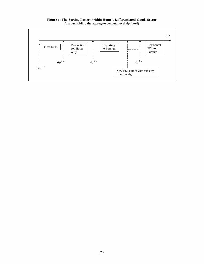
Figure 1: The Sorting Pattern within Home’s Differentiated Goods Sector

(drawn holding the aggregate demand level AF fixed)

a1-ε

aD 1-ε aX

1-ε aI 1-ε

Firm Exits Production for Home only

Exporting to Foreign

Horizontal FDI to Foreign

New FDI cutoff with subsidy from Foreign

aU 1-ε

Figure 2: Welfare as a Function of the Subsidy Level

1.245

1.25

1.255

1.26

1.265

1.27

-0.0

5

0.00

0.05

0.10

0.15

0.20

0.25

0.30

0.35

0.40

0.45

0.50

0.55

Subsidy (sf or sv)

Wel

fare

(WFf

or W

Fv)

Fixed cost subsidy (N exogenous)Fixed cost subsidy (N endogenous)Variable cost subsidy (N exogenous)Variable cost subsidy (N endogenous)

Notes: Parameter values are: k = 3.4, ε = 3.8 (which implies α = 0.74), μ = 0.5, τ = 1.3, fD = 20, fX = 40, fI = 250, fE = 100, aU = 25, wH = wF = 1, and MH = MF = 100,000. These parameter choices imply the order of productivity cut-offs imposed in the model, namely aU > aD > aX > aI . For the graphs where the measure of Home firms is exogenous, the value of N used is that obtained when setting the subsidy level to 0 in equation (25).

26

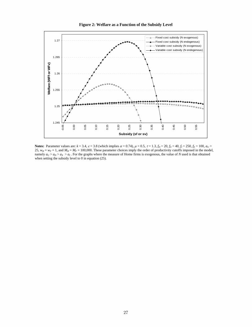
Figure 1: The Sorting Pattern within Home’s Differentiated Goods Sector

(drawn holding the aggregate demand level AF fixed)

a1-ε

aD 1-ε aX

1-ε aI 1-ε

Firm Exits Production for Home only

Exporting to Foreign

Horizontal FDI to Foreign

New FDI cutoff with subsidy from Foreign

aU 1-ε

Figure 2: Welfare as a Function of the Subsidy Level

1.245

1.25

1.255

1.26

1.265

1.27

-0.0

5

0.00

0.05

0.10

0.15

0.20

0.25

0.30

0.35

0.40

0.45

0.50

0.55

Subsidy (sf or sv)

Wel

fare

(WFf

or W

Fv)

Fixed cost subsidy (N exogenous)Fixed cost subsidy (N endogenous)Variable cost subsidy (N exogenous)Variable cost subsidy (N endogenous)

Notes: Parameter values are: k = 3.4, ε = 3.8 (which implies α = 0.74), μ = 0.5, τ = 1.3, fD = 20, fX = 40, fI = 250, fE = 100, aU = 25, wH = wF = 1, and MH = MF = 100,000. These parameter choices imply the order of productivity cutoffs imposed in the model, namely aU > aD > aX > aI . For the graphs where the measure of Home firms is exogenous, the value of N used is that obtained when setting the subsidy level to 0 in equation (25).

27

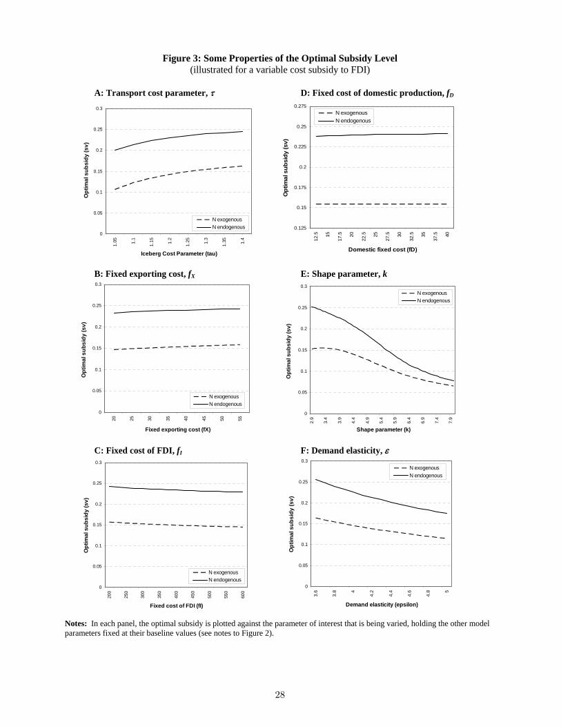
Figure 3: Some Properties of the Optimal Subsidy Level (illustrated for a variable cost subsidy to FDI)

A: Transport cost parameter, τ D: Fixed cost of domestic production, fD

0

0.05

0.1

0.15

0.2

0.25

0.31.

05 1.1

1.15 1.2

1.25 1.3

1.35 1.4

Iceberg Cost Parameter (tau)

Opt

imal

sub

sidy

(sv)

N exogenousN endogenous

0.125

0.15

0.175

0.2

0.225

0.25

0.275

12.5 15

17.5 20

22.5 25

27.5 30

32.5 35

37.5 40

Domestic fixed cost (fD)

Opt

imal

sub

sidy

(sv)

N exogenousN endogenous

B: Fixed exporting cost, fX E: Shape parameter, k

0

0.05

0.1

0.15

0.2

0.25

0.3

20 25 30 35 40 45 50 55

Fixed exporting cost (fX)

Opt

imal

sub

sidy

(sv)

N exogenousN endogenous

0

0.05

0.1

0.15

0.2

0.25

0.3

2.9

3.4

3.9

4.4

4.9

5.4

5.9

6.4

6.9

7.4

7.9

Shape parameter (k)

Opt

imal

sub

sidy

(sv)

N exogenousN endogenous

C: Fixed cost of FDI, fI F: Demand elasticity, ε

0

0.05

0.1

0.15

0.2

0.25

0.3

200

250

300

350

400

450

500

550

600

Fixed cost of FDI (fI)

Opt

imal

sub

sidy

(sv)

N exogenousN endogenous

0

0.05

0.1

0.15

0.2

0.25

0.3

3.6

3.8 4

4.2

4.4

4.6

4.8 5

Demand elasticity (epsilon)

Opt

imal

sub

sidy

(sv)

N exogenousN endogenous

Notes: In each panel, the optimal subsidy is plotted against the parameter of interest that is being varied, holding the other model parameters fixed at their baseline values (see notes to Figure 2).

28