Common Shocks and Currency Crises*

Ramon Moreno and Bharat TrehanFederal Reserve Bank of San Francisco

April 28, 2000

AbstractThis paper attempts to determine the extent to which common external shocks explain

simultaneous currency crises. We define crises on a country by country basis using a new

criterion that takes into account variations in the volatility of exchange rates over time and across

countries. Using a Poisson regression model, we find that over the post-Bretton woods period, a

small number of common external shocks can explain between sixty to eighty percent of the

variation in the total number of crises over time, depending upon the set of countries one looks

at. Our findings provide one explanation of why currency crises sometimes bunch together and

sometimes do not.

* The authors thank Casey Cornwell and Mark Peralta for research assistance. Any opinionsexpressed in this paper are those of the authors and not necessarily those of the Federal ReserveBank of San Francisco or the Federal Reserve System.

1

I. Introduction

The experience of collapsing currency pegs in the 1990s—Europe in 1992–1993, Mexico

in 1994–1995 and Asia in 1997–1998—has stimulated new research into the causes of currency

crises. The fact that the crises occurred simultaneously in a number of countries has drawn

particular attention. One view is that currency crises spread to those countries that are tied

together by international trade (Eichengreen, Rose and Wyplosz, 1997, Glick and Rose 1999).

Another view is that currency crises spread to countries which share common fundamentals, such

as recent credit booms (suggesting weakness in the banking system), real exchange rate

appreciation or are illiquid internationally (Sachs, Tornell and Velasco, 1996 and Tornell, 1999).

While these studies shed light on the common features of the countries that have currency

crises at about the same time, they generally do not have much to say about why the ‘first victim’

experienced a crisis. Nor do they provide an explanation of the variation in the total number of

crises over time, and, in particular, why crises sometimes bunch together and sometimes do not.

This is the task we take up in this paper. More specifically, we try to explain the distribution of

crises over time in terms of common external shocks. Informal observation (and some empirical

evidence) suggests that such common external shocks may be important. For example, the debt

and currency crises in 1982 were preceded by a period of rising U.S. interest rates, sharply

increasing the external debt burdens of heavily indebted developing countries. The European

currency crises of 1992–1993 were preceded by an extended period of deutschemark appreciation

that made it costly for European economies to maintain their linked currency arrangements.

We begin by defining crises on a country by country basis using a new criterion that takes

into account variations in the volatility of exchange rates over time and across countries. This

1 Huh and Kasa (forthcoming) present a theoretical model that is consistent with ourinterpretation of the complementarity between external shocks and country characteristics. Intheir model, adverse external shocks lead to strategic devaluations by a group of countries thatexport to the same markets.

2

measure is then aggregated across (several different sets of ) countries to obtain (several

different) time series on currency crises. Each of these series consists of a count of crises over

time, and we attempt to explain the time series variation in each count in terms of common

external shocks. Since our dependent variable can only take on values that are non-negative

integers, we employ the Poisson regression model for estimation.

Some of our explanatory variables (such as the U.S. interest rate) have been used before,

but in models that attempt to predict the occurrence of a crisis in a given country at a given point

in time. Several other variables are new to this study. These include measures of inflation, third-

country exchange rates and investment flows. We find that common shocks can explain between

sixty to eighty percent of the variation in the total number of currency crises over the post-

Bretton woods period, depending upon the group of countries one is looking at.

Our analysis is concerned with predicting how many countries are likely to be hit by a

currency crisis at a given point in time, given that the impulse takes the form of a common

external shock. We view it as complementary to studies that examine the transmission of shocks

by focusing on how country characteristics (such as debt-income ratios or the amount of bank

lending) determine which countries are likely to be hit by a crisis1. However, our ability to

explain a reasonably large proportion of the time series variation in crises using a small set of

global variables restricts the potential role of explanations in which a domestically-precipitated

currency crisis in a single small country leads to simultaneous devaluations by a group of

3

countries (perhaps because the initial devaluation serves as a coordinating device or “wake up”

call).

The plan of our paper is as follows. In section II we review some of the existing research

on currency crises. Section III motivates our focus upon common shocks and also deals with

some issues having to do with estimation strategy. The empirical analysis in this paper can be

divided into two parts. The first part is in Section IV, where we discuss issues surrounding the

construction of a currency crisis index and present the index that we use. We also present some

comparisons of our index with those proposed by others. Section V contains the second part,

where we try and explain the movements in our index in terms of common shocks. Section VI

concludes.

II Previous research

Most models of sharp depreciations or currency crises focus on domestic conditions that

trigger such crises. These may involve money creation that is incompatible with a pegged

exchange rate because of ongoing budget deficits (Krugman, 1979, Flood and Garber, 1984), or

to prop up a weak financial sector (Calvo and Mendoza, 1996, Corsetti Pesenti and Roubini,

1998, Burnside Eichenbaum and Rebelo, 1998), or situations in which the costs exceed the

benefits of pegging, possibly because the real exchange rate has become overvalued (Obstfeld,

1994, Drazen and Masson, 1994, and Flood and Marion, 1997). Currency crises may also reflect

panics due to illiquidity in even normal financial systems (Chang and Velasco, 1998), or

excessive lending that makes the economy vulnerable to adverse shocks (McKinnon and Pill,

1998).

2 Frankel and Rose (1996) and Milessi-Ferretti and Razin (1998) are exceptions that wediscuss below.

4

In line with this, empirical analyses of episodes of speculative pressure on the exchange

rate are almost always concerned with conditions in individual countries, rather than on global

conditions2. For example, two well known studies by Eichengreen, Rose, and Wyplosz (1995)

and Kaminsky and Reinhart (1999) model the influence of external conditions around episodes of

speculative pressure by focusing on country-specific variables such as foreign reserves, changes

in dollar exports or imports, current account, real effective exchange rate and the interest rate

differential (domestic and foreign). Part of the reason for this emphasis is that researchers have

mainly been interested in describing the conditions that may predict the timing of episodes of

speculative pressure or currency crises in specific countries.

One limitation of this country-focused approach is that it does not directly explain a well

established phenomenon: the (occasional) nearly simultaneous occurrence of crises in a large

number of countries. For example, according to Glick and Rose (1999), in 1973 alone eighteen

countries experienced speculative pressures, reflecting the collapse of the Bretton Woods system.

In 1992, nine countries experienced such pressures, due to the attacks on the exchange rate

mechanism of the European Monetary System. More recently, in 1997, sixteen countries were

affected by currency speculation in East Asia and its aftermath.

Recent research has explored a number of explanations for the bunching of episodes of

speculative pressure. One explanation is that the spread of currency crises reflects country-

specific fundamentals that just happen to be common to several countries at a given point in

time. Sachs, Tornell, and Velasco (1996) and Tornell (1999) study the spread of currency crises

3 Another literature tests for contagion by examining the behavior of asset markets acrosscountries. Thus, Eichengreen, Rose, and Wyplosz (1997), Baig and Goldfajn (1998), Dekle,Hsiao, and Wang (1999) test whether news in a neighboring country affects a country’s exchangerate or asset returns, after controlling for fundamentals. Another approach involves tests todetermine if the covariance of returns increases during periods of market turmoil. Forbes andRigobon (1999) reexamine the evidence in this literature and conclude that high market co-movements reflect cross-market linkages or interdependence, rather than pure contagion.

5

in emerging markets in 1995 and 1997 and find that currency crises spread to countries which

experience credit booms (suggesting weakness in the banking system), real exchange rate

appreciation or are illiquid internationally.

Glick and Rose (1999) offer an alternative explanation. Using data for five different

currency crises they show that currency crises spread to those countries that are tied together by

international trade. They also find that after controlling for trade links, macroeconomic and

financial influences are not closely associated with the cross-country incidence of speculative

attacks, which appears contrary to the findings of Sachs, Tornell, and Velasco (1996) and Tornell

(1999). Eichengreen, Rose, and Wyplosz (1997) reach similar conclusions in a study of

contagion in OECD countries.3

These studies take the “first victim” as given; but it is not clear what, if anything, triggers

the first episode. Perhaps a more fundamental problem is that these studies provide no

explanation for why crises sometimes bunch together and at other times do not. For example, the

sharp depreciation experienced by Thailand in 1997 spread to its trade competitors in the region,

but a similarly sharp depreciation in 1984 did not. For another example, consider the crisis

measure constructed by Frankel and Rose (1996). While there are three years in their twenty year

(eighty country) sample when 10 or more countries have crises, the sample also contains eight

years when there are only 1 to 4 crises per year, and another seven years where the number of

4 The effect of global interest rates on external debt burdens is emphasized by Balassa,1986.

6

crises is between 5 and 9. Clearly, not every crisis leads to contagion or spills over to other

countries.

III. A Role for Common Shocks

One explanation that may account for this pattern but that has received relatively less

attention is the possibility that these countries are being hit by common shocks (global or

regional). It is not hard to imagine scenarios in which such shocks result in simultaneous crises

in a number of countries. A global shock may alter the environment in such a way that a group of

countries who were in no danger of insolvency find their position untenable. A worldwide

disinflationary shock, for example, may make it impossible for primary commodity exporters to

service their existing debt. Thus, Frankel and Rose (p. 356) state that “The debt crisis of 1982,

and subsequent debtor devaluations, were to a large extent triggered by the tight northern

monetary policy which resulted in high interest rates and a global recession.”4 At other times, the

problems may be country specific, with global shocks playing a role largely in the timing of the

crisis. For instance, an increase in global interest rates may serve to coordinate banking system

failures across countries whose systems might otherwise have collapsed at different points in

time. Note that neither of these scenarios denies the importance of country specific factors in

determining exactly which countries are hit by a crisis. For instance, in order to predict whether a

given country was going to be hit under our second scenario, we would need to know something

about the health of its banking sector, just as in Tornell (1999). Finally, as mentioned above,

5 Fernandez-Arias (1996) overturns the conclusion of an earlier study by Chuhan,Claasens and Mamingi (1993) that domestic factors were more important by taking into accountthat country creditworthiness depends on global as well as external factors. Agénor andHoffmaister (1998) confirm that these results carry through in the East Asian context. UsingVAR models, they find that world interest rates have a significant impact on capital flows and thereal exchange rate in Korea, Philippines and Thailand.

7

Huh and Kasa (forthcoming) describe another way in which common external shocks can lead to

simultaneous currency crises.

A number of earlier studies have taken common shocks into account when trying to

explain the timing of crises in individual countries. Generally speaking, these studies have

focused on how shocks to interest rates and output growth in the developed economies affect

capital flows or the incidence of currency crises in developing countries. Writing well before the

recent East Asian currency crises, Calvo, Leiderman, and Reinhart (1996) issued a warning about

capital inflow surges in the first half of the 1990s in both Latin America and East Asia, noting

that external factors driving such flows contain an “…important cyclical component, which has

given rise to repeated booms and busts in capital inflows (p. 124).”

Using principal components analysis, Calvo, Leiderman, and Reinhart (1993) find that

proxies for capital inflows (foreign reserve accumulation and real exchange rate appreciation) to

Latin America were significantly negatively correlated with U.S. interest rates in the early 1990s,

suggesting that external factors were the primary determinant of capital flows in that period. This

was confirmed by Fernandez-Arias (1994), who estimated that global interest rates accounted for

nearly 90 percent of the increase in portfolio flows for the “average” emerging market in 1989-

19935. Studies using panel data over longer sample periods also suggest that U.S. interest rates

6 Agénor (1998) develops an intertemporal optimizing model that spells out theconditions that determine the impact of global interest rate shocks on the real exchange rate of asmall open economy.

7 Casual observation suggests that demand shocks and terms of trade effects may beimportant predictors of crises. For example, the stagnation in oil prices in the early 1980sadversely affected Mexico’s export revenues and output performance, contributing to the debtcrisis Mexico experienced after 1982. Similarly, steep declines in semiconductor prices in thesecond half of the 1990s were followed by currency crises in East Asia in 1997.

8

are important determinants of capital flows or currency crises (Milesi-Ferretti and Razin,1998,

Frankel and Rose, 1996).6

The evidence on the implications of output growth for currency crises is mixed. Milesi-

Ferretti and Razin (1998) find evidence that slower output growth is associated with an increased

probability of crises. However, Frankel and Rose (1996) find this to be the case in only one of

three sets of regressions that they present. These findings reflect the theoretical ambiguity of the

effects of global economic activity on the incidence of crises. On the one hand, a decline in the

growth of industrial countries tends to reduce the incidence of crises by increasing capital flows

to small open economies. On the other hand, the reduction in growth tends to increase the

incidence of crises through its unfavorable effect on demand and the terms of trade in these

economies. This may make it difficult to maintain a currency peg by raising unemployment, and

by making it more difficult for a country to service its foreign debt.7

While existing research provides important insights on how external shocks may

influence capital flows and currency crises, there appears to be scope for further empirical

analysis of this question. For example, it is generally believed that the appreciation of the

deutschemark against the U.S. dollar starting in the late 1980s set the stage for the wave of

speculative attacks experienced by currencies linked to the deutschemark via the Exchange Rate

8 To see how big the list of potential candidates can be, one only needs to compare the setof variables used by Frankel and Rose (1996) with that used by Tornell (1999).

9

Mechanism of the European Monetary System. Yet we are unaware of any systematic

examination of the role that major-currency fluctuations might play in causing simultaneous

crises in a number of countries.

In order to focus on the role played by common shocks in the distribution of crises over

time, we suppress the variation in crises across countries. We do so by adding up the number of

crises across countries at each point in time, so that we end up with a time series of crises. Given

a large enough sample, the number of crises due to independent country-specific factors should

be approximately constant over time. Based on this assumption, we will try and explain the

variation in the aggregate number of crises over time in terms of common shocks. To the extent

that we are unable to do so, we will leave the door open for explanations such as those based on

‘contagion’, which we take to mean explanations where random developments in some (small)

country can lead to simultaneous crises in other countries.

An important benefit of our approach is that by suppressing the cross country variation in

crises we do not have to take a stand on the set of country specific variables that is best at

predicting which country will have a crisis8. However, the decision to aggregate data across

countries rules out the most common method of estimating crisis equations–probit regressions on

panel data that include all possible determinants of currency crises. We provide more details of

the estimation procedure we employ below.

9 Girton and Roper (1979), for instance, propose an index in which the weights reflectthe sensitivity of the exchange rate to changes in foreign reserves. Construction of the indexrequires knowledge of the underlying money demand parameters, which are often unstable anddifficult to estimate. Weymark (1998) generalizes the Girton-Roper method in a way that is lessdemanding in terms of information needed, but the approach still requires more information thanthe alternatives currently in use.

10

IV. Defining Crises

One of the key questions to be addressed in the analysis of exchange rate crises is how to

identify indicators of speculative pressure in foreign exchange markets, and to decide under what

conditions the movement in these indicators represents a “crisis.” The most obvious indicator is

the behavior of the foreign exchange rate. If a country’s exchange rate is floating, or if a peg has

collapsed, a sharp depreciation is an unambiguous indicator of a shift in sentiment or speculative

pressure against a currency.

If exchange rate stability is maintained, however, pressure on the exchange rate will be

reflected in other ways. If investors want to switch away from a country’s assets, the exchange

rate will tend to depreciate and a country’s central bank may respond in two ways to prevent

depreciation. First, it may seek to sell foreign reserves, to accommodate the increased demand for

foreign assets. Second, it may allow interest rates to rise. Thus, the depletion of foreign reserves

or increases in interest rates can serve as indicators of speculative pressure. Examples where such

variables would provide information not given by the exchange rate are Argentina’s costly efforts

to defend its peg in 1995, and similar efforts by Hong Kong in 1998.

While some researchers have proposed indexes that use an explicit analytical framework

to weight the different sources of exchange rate pressure discussed above, such measures are not

easy to construct9. Consequently, empirical researchers have resorted to simpler, ad hoc

11

weighting schemes. For example, in their study of currency crises in OECD countries,

Eichengreen, Rose, and Wyplosz (1995) employ weights that adjust for differences in the

volatility of the components of the index to ensure that the units (exchange rate, foreign reserve,

or interest rate changes) are comparable. Implicit in this approach is the assumption that a one

standard deviation change in the interest rate represents as much of a currency crisis as a one

standard deviation change in exchange rates or reserves.

Another difficulty is that data for some of the indicators of exchange market pressure are

often not available. For example, Kaminsky and Reinhart (1999) construct an index similar to

Eichengreen, Rose, and Wyplosz (1995), but exclude interest rates because market-determined

rates are not consistently available for even their 20 country sample. Working with a set of 91

developing countries, Frankel and Rose (1996) go a step further and construct an indicator based

on the behavior of foreign exchange rates alone, on the grounds that foreign reserve data contains

a lot of noise. A recent example can be found in the Thai crisis of 1997: The Bank of Thailand

suffered heavy losses in the forward market trying to defend the Thai baht peg, but since these

were off-balance-sheet transactions they were not fully reflected in the official statistics.

Another question that needs to be addressed is when a movement in an indicator of

speculative pressure constitutes a crisis. Researchers have come up with a number of different

criteria. Eichengreen, Rose, and Wyplosz (1995) identify a crisis whenever the change in their

index is two standard deviations above the mean. Kaminsky and Reinhart (1999) use a similar

rule, but compute separate standard deviations for episodes when annualized monthly inflation

exceeds 150 percent. Frankel and Rose (1996) use an absolute cutoff. As suggested by

Kaminsky and Reinhart’s (1999) adjustment for high inflation episodes, one disadvantage of

10 See the data appendix for a description of the data.

12

using standard deviations computed over a full sample is that “too many” crises may be

identified during periods when the exchange rate is very volatile.

As is apparent from the preceding discussion, no measure of currency crises is perfect.

After weighing the pros and cons of the alternative approaches, we opted for a measure of

speculative pressure based on the behavior of the exchange rate alone. The main reason is that we

would like to predict the global incidence of currency crises, which suggests the use of an index

that maximizes the number of countries in our sample. Using data on exchange rates, we ended

up with a sample of 121 countries over the (post-Bretton woods) 1974-1997 period; by contrast,

we could find foreign reserve data for 85 countries only.10

In formulating a crisis rule, we specifically attempt to accommodate changes in the

variability of exchange rates, as it is apparent that exchange rate volatility tends to vary over time

and across countries. Thus, the rule we employ declares a currency crisis if the change in the

exchange rate in a given quarter exceeds the average change over the past five years by two

standard deviations (measured over the same period). One advantage of this definition is that we

do not have to respecify the condition to deal with high inflation episodes.

Obviously, elements of arbitrariness remain. When computing the standard deviation,

should we look at data over the last five years? Or two? Or ten? Similarly, is an event large if it

exceeds two standard deviations or three? To answer these questions we looked at how the set of

crises detected by the rule changed in response to changes in these criteria. For instance, a move

to three standard deviations essentially eliminated the 1992 crisis in Europe, so we decided to

retain two standard deviations as the cutoff. Also, in the course of this examination we discovered

11 Since our definition of currency crises in terms of the recent variability of exchangerates is new to the literature, we also explored the properties of a measure based on a morefamiliar definition, one that is related to Frankel and Rose’s (1996). Specifically, a crisis was saidto occur if the annualized change in a given quarter’s exchange rate exceeded the rate of inflationover the prior year by 40 percent, and if the quarter’s depreciation exceeded the previousquarter’s by 20 percent. The subsidiary condition is meant to rule out cases of relatively large, butsteady, deviations. As in the first criterion, we ruled out two crises within the same year in anycountry. We found that this measure found too many crises in the latter part of our sample(probably because of an increase in exchange rate volatility over time), and decided against usingit in the subsequent analysis.

13

that our criterion would sometimes find crises where a brief sudden appreciation was followed by

a sharp depreciation. Since these short-term reversals appear to reflect volatility in currency

markets that has no lasting implications, we decided to include a subsidiary condition which

ensures that a currency crisis is only declared if the value of the currency at the end of the crisis

quarter is below where it was a year ago. Finally, we also imposed a window to ensure that no

country had two crises within a 4 quarter period, by dropping the three quarters following a crisis

from the sample.11

As discussed at the end of the previous section, we aggregate our currency crisis index

over countries in order to obtain a count of the total number of crises occurring per year.

Aggregating crises in this way gives us a straightforward way to examine our crisis index. The

crisis measure (CCE ) for our 121 country set is shown in Figure 1 (panel A). We also distinguish

between currency crises in developing and developed countries. Panel B shows crises in the

former, where the set of developing countries is that defined by Frankel and Rose (1996), while

panel C shows crises in the set of countries that were members of the OECD in 1975. To further

illustrate its properties, we show our measure aggregated over the twenty countries studied by

Kaminsky and Reinhart , as well as the Asian economies as grouped by the IMF (panels D and E).

14

In panels B and D we include the actual crisis measures used by Frankel and Rose, and Kaminsky

and Reinhart, for purposes of comparison.

Turning to panel A, our global measure has peaks in the mid-1970s, the early 1980s and

the early 1990s. The OECD set (panel B) shows the currency crisis of the early 1990s (which is

the dominant crisis in the OECD set), while the 1997 crises dominate the series for Asia. The

correlation between our measure and the Frankel and Rose measure (for the Frankel and Rose

country set) is 0.68, though our measure shows more crises than the Frankel and Rose measure

after the early 1980s. An important reason that the original Frankel and Rose measure does not

show an increase in crises during the latter period is that it is based on a rule that permits no more

than one crisis per country every four years. The correlation between our measure of crises and the

Kaminsky-Reinhart measure (for their set of countries) is 0.67; panel D shows that the two

measures are most closely related during the 1990s.

The peak in crises around 1975 (see panel A) has not previously been reported in the

literature. To see whether such a peak could be identified by other means, we checked the IMF

Report on Exchange Rate Arrangements and Exchange Rate Restrictions for 1976, and found that

close to half the countries identified as having a crisis or sharp depreciation episode in 1975 had

implemented explicit currency realignments (devaluations or re-pegging from one currency to

another). About half of the remainder were pegged to sterling, which experienced a steep drop

against the dollar in 1975. Several others used the rand as their national currency, and this

currency was realigned in 1975 as well.

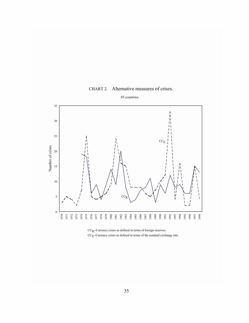
As another check, Figure 2 plots a measure of crises based on foreign reserves (CCR)

against CCE. Because of data limitations, the CCR series begins in 1975, and also contains a total

15

of 85 countries only. However, it shows a peak in 1975 as well, and generally moves pretty

closely with CCE (which is calculated for the same sample of countries here). The exception is

1992, when CCE shows a marked peak that is not reflected in CCR. An examination of the

individual components shows that the reserves based measure fails to pick up many of the

European countries that were affected by the ERM crisis, so we interpret the discrepancy in 1992

as indicating more of a problem with CCR than CCE.

V. Predicting Crises

1. Estimation Technique

The data we are trying to predict is a series of counts: the number of crises in the world

during a year. The estimation technique we employ needs to take this into account; specifically, it

needs to account for the fact that the dependent variable is an integer which cannot be negative.

This rules out least squares estimation; instead, we will use the Poisson regression model. Thus,

we assume that—conditional on the set of regressors xi—the density of our crisis variable c i is

given by

f c x ec

ci iic

ii

i i

( ) , , , ,....!

= =− µ µ 0 1 2

and that its mean is given by

E c xi i i[ ] , = = eci'

µ β

16

which ensures that is greater than zero.µi

A characteristic of the Poisson distribution is that the variance is equal to the mean, so that

the conditional variance of c is nonconstant. Note also that

∂

∂β βE c x

xe x( ) ( )=

so that the effect of a change in x on c does not equal the regression coefficient .β

The equations are estimated using maximum likelihood.

2. Interest Rates, Output and Inflation

In identifying global variables that may predict crises, we take the literature cited earlier as

a starting point, that is, we begin by looking at the role played by global interest rates and

variations in economic activity in explaining crises.

As discussed above, an increase in global interest rates can matter for a variety of reasons.

For instance, higher interest rates will raise the cost of servicing variable rate debt, and therefore

raise doubts about a country’s abilities to meet its external obligations. Or it may cause an outflow

of funds which policymakers in a small open economy may find too costly to counter by raising

domestic interest rates, resulting in a currency collapse. The reasons for the reluctance to raise

rates may be high domestic unemployment, or a weak domestic banking system.

Considerations such as these imply a role for interest rates, but do not provide firm

guidance about which measure to include. If the focus is on U.S. monetary policy shocks, one can

include U.S. short term rates, as Frankel and Rose do. However, we have decided to use the U.S.

12 See, for instance, Mishkin (1997) and the references there.

17

triple-A corporate bond rate instead. A long term corporate rate is likely to be more sensitive to

perceptions of risk in the economy and to provide a better measure of inflation expectations than

a short term rate.

Interest rates alone do not seem to be enough to capture the different kinds of shocks

associated with variations in global economic activity. In response, researchers have used

measures of output growth to explain crises. In our own analysis, we did not find convincing

evidence of a role for output shocks (we will discuss this below); we did, however, find more

convincing evidence for inflation shocks. This evidence is consistent with several accounts of the

role played by U.S. monetary policy in the debt crises of the early 1980s (recall the statement by

Frankel and Rose cited above). To see how such a shock might work, consider what would

happen following a deflationary shock in the U.S. The direct effect of such a shock would be to

lower export revenues and consequently economic activity in countries that export to the U.S. The

resulting unemployment would make it more difficult for them to maintain a pegged currency (as

in Obstfeld, 1994, Drazen and Masson, 1994).

Another effect would work through a debt channel. In the case of a closed economy, a

number of papers have shown that changes in inflation can cause problems for borrowers, and that

these problems can be large enough to have substantial effects on the macroeconomy12. The same

considerations apply with regard to the burden of external debt in open economies. For example, a

disinflationary shock that lowered the demand for exports and their prices would raise the burden

of debt even if nominal interest rates—and therefore nominal payments—were held fixed. Thus,

disinflation in a major economy (such as the U.S.) could be associated with an increase in the total

13 As a check on our results, we did estimate the regressions in Table 1 below with theinflation-surprise specification, where annual U.S. inflation was modeled as an AR(2) processestimated over the whole sample period. The results were about the same as those shown inTable 1; this may reflect the fact that for much of this period inflation is close to a random walk.

18

number of crises. Commodity exporters, in particular, are likely to be hit hard by such a

development.

These considerations argue for including a variable measuring inflation in our crises-

prediction equation. Once again, we have opted to stay with a measure of U.S. inflation. A related

question is whether it is the change in inflation or the unpredicted component of the change in

inflation that matters. While certain kinds of models suggest working with inflation surprises, we

have decided to go with the change in inflation (in part because of the difficulty in determining

how exactly to define an inflation surprise).13

Table 1 shows the results for regressions that include (the log of) interest rates and the (log

of the) inflation rate. We have included a contemporaneous value and a lag for both these

variables. In the first column we impose the restriction that the coefficient on the lag is the same

size as the coefficient on the contemporaneous term, but has the opposite sign. The data do not

reject this restriction for either variable at the 10 percent level. Both variables can thus be entered

as changes; we have retained levels to allow for comparability across specifications where this

restriction is rejected by the data. The estimates in Table 1 show that an increase in the interest

rate leads to an increase in crises. Under the assumption that interest rates are a random walk, this

implies that it is interest rate surprises that matter for crises, and not the level of interest rates.

Similarly, it is the change in the inflation rate that matters, and not the level. These results are

consistent with the debt deflation story above.

14 The R2p measure compares the fit of the model with that provided by a model with only

a constant term. It can be negative and also fall when variables are added to the model. Whenthe model is estimated by MLE, R2

d measures how much the fit improves in going from a modelthat contains only a constant term to the given model relative to the improvement in going from amodel that contains only a constant term to the perfect model. Thus, it is bounded between 0 and1. See Greene (1997).

15 If the restriction that the mean equal the variance were rejected, we would have toemploy an alternative estimation strategy. See Cameron and Trivedi (1998) for a discussion.

19

Turning to the goodness-of-fit measures, the Chi-square statistic shows that the set of

explanatory variables (taken together) is highly significant. Since the equation is nonlinear, one

cannot use the usual R2 measure; we report a couple of pseudo-R2 measures instead14. These

measures are both about 0.5, suggesting that the two variables do a reasonably good job of

explaining the variation in currency crises over time. It is worth pointing out that the inflation

surprise variable is responsible for most of this; when only interest rates are included, the pseudo-

R2 s are just below 0.1. Finally, the overdispersion test shown at the bottom of the table is based

on a specification that the variance equals k times the mean. We are unable to reject the null that k

equals 1.15

The remaining two columns of the table show the results for two subsets of our sample.

The first subset contains the countries that were in the OECD in 1975. The coefficients in the

second column (for the OECD) have the same signs as in the first column. However, the interest

rate variables are no longer significant at conventional levels (and dropping the inflation terms

actually leads to a negative R2p ). The pseudo-R2 are about half those for the first equation. The

second subset (the results for which are shown in the third column) contains the 91 countries

classified as “developing” by Frankel and Rose (1996). Our specification performs about as well

for the developing country set as it does for our full sample. The pseudo-R2s indicate a reasonably

20

good fit, though the t-test suggests a tendency towards overdispersion, as it is significant at 10, but

not at 5, percent. As was the case in the full sample regression, excluding the inflation variable

reduces the pseudo-R2 to less than 0.1. Overall, our results suggest that variations in global

interest rates and inflation are much more important for explaining crises in developing countries

than in the OECD.

Given the importance attached to the output growth variable in earlier studies, it seems

useful to describe what happened when we included this variable in our equation before

concluding this section. Echoing the findings of Frankel and Rose (1996), we found that U.S.

income growth did not help explain crises in the developing countries. Output growth did matter

for the OECD countries (and for the aggregate index). A closer look revealed that the explanatory

power of the output variable had to do largely with its ability to explain the 1992 crises. We found

it hard to understand this result, and so decided to drop the output variable.

3. Third country exchange rates

Although previous empirical work has not paid much attention to the role of third country

exchange rates in contributing to currency crises, it is not hard to see why movements in the

bilateral exchange rates of large economies might trigger such crises. Countries that peg to a

major currency will experience a trade-weighted appreciation if that currency appreciates. As is

well known (Flood and Marion, 1997, Kaminsky and Reinhart, 1999), such appreciation is often

followed by sharp depreciations or currency crises. The crisis in the exchange rate mechanism

(ERM) of the European Monetary System in 1992 is consistent with this description, since it was

preceded by an extended period of deutschemark appreciation.

16 We repeated the regressions below using exchange rate changes over a 3 year period(instead of the 4 year period in the text) and obtained similar results.

21

Note that common currency shocks are likely to have effects that would satisfy the

conditions that have been taken as evidence of spillovers (for example, by Glick and Rose, 1999).

An appreciation of the deutschemark, for instance, would cause the currencies that were linked to

it to appreciate, and would cause the associated economies to slow (with a loss in trade

competitiveness playing a role in the slowdown). Domestic conditions may then force a

devaluation in many of these countries. Since it is likely that these countries have similar trading

patterns (after all, they do peg to the same currency), tests that look for evidence of spillovers

based on trading patterns are likely to find it, even though the underlying cause of depreciation is

a common shock.

Table 2 adds bilateral exchange rates to the interest rate and inflation variables in Table 1.

We include two exchange rates: the mark-dollar rate and the yen-dollar rate. To eliminate the

effects of short run volatility we look at the effect of cumulative changes over a four year span16.

Also, the dollar has shown a trend depreciation over the sample period (especially against the

yen); thus, a one yen change (for example) represents a much larger percentage change at the end

of our sample than at the beginning. Consequently, we include the change in the log of the

exchange rate. Finally, to avoid simultaneity problems, we lag this variable by one year.

The table shows that neither exchange rate variable is significant in the aggregate

equation; however, both are significant in the other two equations (at 10 percent for developing

countries, and at 1 percent for the OECD countries). These findings may be reconciled by

17 Note also that with the mark-dollar rate held fixed, a change in the yen-dollar rate isreally a change in the mark-yen rate.

22

observing that each of the exchange rates has the opposite sign in the two equations, so the effects

are likely to cancel on the aggregate.

In the OECD equation, the coefficient on the deutschemark (Dmchg) is negative, and on

the yen (Yenchg) is positive. Thus, a sustained appreciation of the mark (a decrease in DMchg)

leads to an increase in crises in the OECD countries, a result which is consistent with the

description of the 1992 crisis above. On the other hand, an appreciation of the yen (a decrease in

Yenchg) reduces the crises in OECD countries, which is intuitive since these countries compete

with Japan.17 Inclusion of the bilateral exchange rates leads to an approximate doubling of the

pseudo-R2, from about .25 in Table 1 to about .5 in Table 2.

In the developing countries equation, the coefficient on the deutschemark is positive, while

that on the yen is negative. Thus, a mark appreciation leads to fewer crises in the developing

countries, which is understandable given the large set of countries that tend to peg to the dollar

rather than the deutschemark and trade with European countries whose currencies are linked with

the deutschemark. In contrast, a yen appreciation increases the number of crises in developing

countries. This coefficient is difficult to explain in the context of East Asian developing

economies whose currencies appear to experience depreciation pressures during periods of yen

depreciation. However, developing countries in Africa or Latin America are unlikely to face the

same pressures. As a comparison of panels B and E in Chart 1 indicates, the yen depreciation in

the period up to 1997 appears to have been far more significant for Asia (where it is associated

with a global peak in the currency crisis measure) than for the set of developing countries as a

23

whole (where the value of the crisis measure in 1997 is less than half as much as the global peak).

In any event, the exchange rate variables are only marginally significant in the developing country

equation, and do not lead to any improvement in either the pseudo-R2 or the result of the

overdispersion test.

4. Capital flows

While our results up to this point suggest that shocks to U.S. interest rates and inflation, as

well as movements in major currency exchange rates, account for a large proportion of the

variation in the incidence of currency crises, much of the recent discussion of currency crises does

not emphasize these channels. Instead, many commentators have emphasized the role played by

capital flows.

One well known story is based on “boom and bust” cycles in capital flows. As discussed

by Calvo, Laderman, and Reinhart (1996), there have been a number of episodes in which

international capital flows to developing countries increased sharply for a number of years and

then suddenly reversed direction, precipitating crises in the recipient countries. While these

authors emphasize the role of shocks to global interest rates in inducing such reversals and crises,

the cumulative value of such flows may influence the incidence of crises separately from the

effect of global interest rates. At least two reasons may be offered for this. First, these funds may

be used to finance risky investments (McKinnon and Pill, 1998, Corsetti, Pesenti, and Roubini,

1998, Tornell, 1999), the impact of which will be larger the larger their cumulative value. The risk

of crises may be accentuated if for some reason borrowers do not or cannot hedge their foreign

currency exposure. Second, as the cumulative stock of external financing rises, the benefit to

18 For a model describing the incentives for debt repayment, see Eaton and Gersovitz,1981.

19 Milesi-Ferretti and Razin (1998) show that the lagged 3-year average value of thecurrent account of a middle-income country helps predict whether it will have a currency crisis(in some specifications).

24

defaulting on external debt goes up, so that an adverse external shock is more likely to trigger

defaults and related currency crises (because such a shock can raise the cost of repayment above

the penalty for defaulting on external debt).18

The data we use to determine whether investment flows matter is from the IMF’s balance

of payment statistics. To emphasize the acquisition or liquidation of foreign assets, we focus on

gross outflows. These are further broken down into direct, portfolio and “other flows.” For most

of the analysis to come, we use the “other flows” component. This component is dominated by

bank lending, and its use reflects our beliefs about the role of banks in crises episodes. For

instance, the 1997 crises in Asia were to a large extent the result of uncertainty about the

willingness of commercial banks to roll over loans that were maturing. This is consistent with the

argument of Chadha and Folkerts-Landau (1999), who point out that while the share of banks in

international capital flows has declined, they continue to play a key role, particularly in emerging

markets.

To look for boom-and-bust effects, we include the sum of investment flows over the

previous four years19. The idea is that during lending booms this variable will become unusually

large. So the hypothesis is that large values of this variable should be followed by an increase in

crises. Table 3 shows that when this variable is included in our specification it is significant only

in the aggregate and developing country equations, indicating that sustained increases in

25

investment flows are followed by an increase in currency crises in developing countries but not in

the OECD. We find these results plausible. One reason why developing countries which

experience large inflows may be more vulnerable to crises is that they are unable to borrow in

their own currencies, and therefore cannot fully hedge their external debt (Eichengreen and

Hausmann, 1999).

Capital flows can matter for other reasons as well. For instance, some commentators have

suggested that Thailand’s 1997 crisis spread to other East Asian economies because the collapse

of the Thai currency triggered a generalized “flight to quality.” Similar shifts in the international

allocation of portfolios have been observed in other contexts, such as in the aftermath of the Gulf

War of 1990.

Consequently, we have included an additional variable in Table 3: the lagged change in the

amount of “other” foreign investment by U.S. residents (denoted ∆Invfl). The inclusion of this

variable is variable is meant to capture shifts in the supply of funds, shifts that are not correlated

to changes in interest rates, inflation and major currency exchange rates. To the extent that these

supply shifts represent exogenous shifts in preferences—such as a desire to increase portfolio

diversification—the ∆Invfl variable is similar to the variables that we have already included in

our analysis. However, this may not always be the case. In the Thailand example above, a shock to

a single small country ends up affecting everyone because it affects international capital flows. In

that case, ‘contagion’ can look like a common shock to capital flows.

Nevertheless, we have decided to include this variable in our analysis. One reason is that it

has some important implications for the other coefficient estimates in our regressions. In

particular, note that the “flight to quality” story implies that funds would flow back to the U.S.

26

(and other countries not experiencing crises), causing U.S. interest rates to decline. Thus, falling

U.S. interest rates can sometimes be associated with a withdrawal of liquidity from foreign

markets, instead of an injection, as is commonly assumed in the literature. Consequently, attempts

to measure the effects of interest rate shocks on currency crises without controlling for the effects

of such shifts will lead to biased coefficients.

When the supply shift variable (∆Invfl ) was included in our regressions, it had the

expected sign, with a decrease in investment flows out of the U.S. in a given year led to an

increase in currency crises the following year. However, the marginal significance level of this

term varied between 1 percent (in the OECD equation) and 20 percent. Addition of a second lag

led to the first lag becoming insignificant in all cases, while the second one was highly significant.

Since we only have a limited number of degrees of freedom, we decided to drop the insignificant

first lag and report the results with the second lag only. Table 3 shows that ∆Invfl is significant in

all three equations, and that it has the largest effect on the OECD countries.

Several other results in Table 3 are worth pointing out as well. Note first that the inclusion

of the investment flow variables increases the size of the interest rate coefficients (relative to

Table 2) in line with the discussion on omitted variables above. Second, the inclusion of these

variables leads to a noticeable improvement in fit, with the pseudo-R2s going up by between 0.10

and 0.25. Chart 3 shows actual and fitted values from each of the equations, in order to provide

another measure of their performance.

We have tested the robustness of the results in Table 3 across several dimensions. First, we

employed flows accumulated over three years rather than four. Second, we lagged this 3-year

measure an additional year. Finally, we used the measure for total investments (that is, the sum of

27

portfolio flows, direct investment and the “other” component) instead of the “other” component.

None of these substitutions leads to a noticeable change in the overall results.

5. An Alternative Measure of Crises for Developing Countries

In Table 4 we show how the variables we have employed here perform when we use the

crisis measure devised by Frankel and Rose (1996). (This measure is shown in panel B of Chart

1.) Their sample extends over the period 1973–1992. As we are missing data on cumulative

investment flows for 1973, the first column reports the results without the investment flow

variables. The interest rate variable is significant at 10 percent, all others at 1 percent. All

variables have the same signs as before; the pseudo-R2 measures are about 0.5. The second

column estimates the model over 1974–1992 and includes the investment flow variables. The

cumulative investment variable is significant at 1 percent; however, the flow variable is not

significant. Even so, the pseudo-R2 measures are above 0.65. In neither specification is

overdispersion a problem.

For comparison purposes, the final column of the table shows what happens when we use

our measure of currency crises and estimate the equation for the same set of (developing)

countries and over the same (1974–1992) period. The goodness of fit statistics indicate that our

set of common shocks explains more of the variation in the Frankel-Rose measure of crises than

in the measure constructed in this paper. In addition, a comparison of the coefficients in the last

two columns indicates that (with one exception) the Frankel-Rose measure of crises is more

responsive to common shocks than our measure. This suggests that our finding that external

28

shocks play an important role in causing currency crises is not an artifact of the procedures we

have employed to define currency crises.

It is also useful to assess the sensitivity of our results to changes in the length of the data

sample by comparing the last column of Table 4 with the middle column of Table 3. This

comparison suggests that the addition of the last 5 years of data does not lead to much of a change

in the coefficients of the developing country equation. As might be expected, the smaller sample

has larger standard errors, which causes some of the coefficients in the developing country

equation in Table 4 to become insignificant.

VI. Conclusions

Recent empirical research has focused on the transmission of crises across countries.

Relatively less attention has been paid to what initiates such crises, and, importantly, to why some

crises spread, and others do not. To address these issues, we have suppressed the cross-country

variation in the data, and tried to explain the bunching of currency crises in time using common

shocks alone. We find that a relatively small number of common external shocks can explain a

fairly large proportion of the variation in the total number of crises over time. In common with

earlier studies, we have found a role for global interest rates in causing currency crises in

developing countries. However, our focus on the global incidence of crises allows us to measure

more directly the role that such shocks play in the concentration of such crises at any given point

in time. We have also found a role for some other shocks that had not been previously examined

in the empirical literature, including inflation shocks and third-country exchange rates. Inflation

and nominal interest rates alone can explain about half the variation in our full sample (though

29

they play a noticeably smaller role in explaining crises in the OECD). Adding exchange rates and

investment flows allows us to explain close to three fourths of the variation in the full sample, and

between 60 to 80 percent in our two sub-samples.

We view our work as complementary to recent research on the transmission of crises

across countries. In particular, our findings do not rule out transmission channels such as trade

links, or common financing links emphasized in the literature, but they do suggest that the extent

of transmission—how far “contagion” spreads—may depend upon the aggregate shock hitting the

world economy. Our approach helps explain why not all crises are equally contagious; and

clarifies what causes the “first victim” in a contagious crisis episode to succumb, filling a gap in

existing empirical research. Finally, our ability to explain a reasonably large fraction of the time

series variation in crises using a small number of common shocks suggests a relatively limited

empirical role for contagion or spillover models in which purely domestic developments in one

(small) country are the trigger for simultaneous currency crises in a group of countries.

30

Table 1

Dependent Variable: Number of Currency CrisesSample period: 1974–1997

All Countries OECD Countries Developing Countries

Constant 2.46(.00)1

2.92(.00)

2.73(.00)

3ARatet 3.26 a(.00)

1.58(.46)

4.10 a(.00)

3ARatet-1 -3.26 a(.00)

-3.39(.14)

-4.10 a(.00)

Inft -1.64 a(.00)

-1.79(.02)

-1.94(.00)

Inft-1 1.64 a(.00)

2.78(.00)

1.64(.00)

Chi-Sq 2 67.70(.00)

28.01(.00)

54.76(.00)

R2p 3 .51 .22 .53

R2d 3 .48 .27 .46

t-test for overdispersion 4

1.65(.11)

1.18(.25)

1.87(.07)

Notes: a Contemporaneous and lagged coefficients are restricted to be equal but of opposite sign.The restriction is not rejected at 10%.

1 Marginal Significance Levels are shown in parentheses.2 Tests the hypothesis that all three explanatory variables belong in the equation.3 Pseudo R-squared; for a description, see text.4 See text for discussion.

31

Table 2

Dependent Variable: Number of Currency CrisesSample period: 1974–1997

All Countries OECD Countries Developing Countries

Constant 2.48(.00)1

1.06(.00)

2.18(.00)

3ARatet 3.37 a(.00)

8.94 a(.00)

2.78 a(.00)

3ARatet-1 -3.37 a(.00)

-8.94 a(.14)

-2.78 a(.00)

Inft -1.61 a(.00)

-1.94 a(.00)

-1.65 a(.00)

Inft-1 1.61 a(.00)

1.94 a(.00)

1.65 a(.00)

DMchgt-1 0.04(.88)

-2.95(.00)

0.64(.06)

Yenchgt-1 .11(.80)

7.30(.00)

-0.87(.07)

Chi-Sq 2 67.90(.00)

49.15(.00)

55.00(.00)

R2p 3 .51 .52 .51

R2d 3 .49 .48 .46

t-test for overdispersion 4

1.66(.11)

1.07(.29)

1.93(.07)

Notes: a Contemporaneous and lagged coefficients are restricted to be equal but of opposite sign.The restriction is not rejected at 10%.

1 Marginal Significance Levels are shown in parentheses.2 Tests the hypothesis that all three explanatory variables belong in the equation.3 Pseudo R-squared; for a description, see discussion of Table 1 in text.4 See text for discussion.

32

Table 3Dependent Variable: Number of Currency Crises

Sample period: 1974–1997

All Countries OECD Countries Developing Countries

Constant 4.71(.00)1

0.80(.00)

4.71(.00)

3ARatet 4.93(.00)

11.73 a

(.00)4.13(.00)

3ARatet-1 -6.12(.00)

-11.73 a

(.00)-5.45(.00)

Inft -2.04a

(.00)-2.54a

(.00)-2.12a

(.00)

Inft-1 -2.04a

(.00)2.54a

(.00)2.12a

(.00)

DMchgt-1 -3.70(.00)

0.78(.02)

Yenchgt-1 7.82(.00)

-1.16(.04)

CumInvflt-1 .27(.00)

0.26(.00)

∆Invflt-2 -.94(.00)

-2.01(.00)

-0.75(.00)

Chi-Sq 2 101.17(.00)

72.11(.00)

73.82(.00)

R2p 3 .74 .79 .63

R2d 3 .72 .70 .61

t-test for overdispersion 4

.94(.36)

.81(.43)

1.00(.33)

Notes: a Contemporaneous and lagged coefficients are restricted to be equal but of opposite sign. The restriction is not rejected at 10%.

1 Marginal Significance Levels are shown in parentheses. 2 Tests the hypothesis that all three explanatory variables belong in the equation.3 Pseudo R-squared; for a description, see discussion of Table 1 in text.

33

Table 4Dependent Variable: Currency Crises in 91 Developing Countries

Frankel-Rose measure Our measure

Sample: 1973-1992 Sample: 1974-1992 Sample: 1974-1992

Constant 1.36(.00)1

7.92(.03)

4.73(.00)

3ARatet 1.66a

(.10)4.92(.00)

3.67(.00)

3ARatet-1 -1.66a

(.10)-8.44(.00)

-4.99(.01)

Inft -1.26a

(.00)-2.75a

(.00)-2.02a

(.00)

Inft-1 1.26a

(.00)2.75a

(.00)2.02a

(.00)

DMchgt-1 2.13(.00)

2.81(.01)

0.92(.27)

Yenchgt-1 -2.80(.00)

-3.64(.00)

-1.32(.10)

CumInvflt-1 0.75(.00)

0.24(.13)

∆Invflt-2 -0.37(.25)

-0.65(.01)

Chi-Sq 2 29.43(.00)

42.26(.00)

52.69(.00)

R2p 3 .56 .72 .56

R2d 3 .47 .67 .55

t-test for overdispersion 4

0.98(.33)

-0.57(.58)

1.0(.30)

Notes: a Contemporaneous and lagged coefficients are restricted to be equal but of opposite sign. The restriction is not rejected at 10%.

1 Marginal Significance Levels are shown in parentheses. 2 Tests the hypothesis that all three explanatory variables belong in the equation.3 Pseudo R-squared; for a description, see discussion of Table 1.

34

A. Full s ample : 121 countrie s .

0

5

10

15

20

25

30

35

40

45

1970

1971

1972

1973

1974

1975

1976

1977

1978

1979

1980

1981

1982

1983

1984

1985

1986

1987

1988

1989

1990

1991

1992

1993

1994

1995

1996

1997

1998

Num

ber

of c

rise

s

B. Developing countries (Frankel-Rose).

0

5

10

15

20

25

30

35

1970

1971

1972

1973

1974

1975

1976

1977

1978

1979

1980

1981

1982

1983

1984

1985

1986

1987

1988

1989

1990

1991

1992

1993

1994

1995

1996

1997

1998

Num

ber

of c

rise

s

C. OECD countries.

0

2

4

6

8

10

12

14

16

1819

7019

7119

7219

7319

7419

7519

7619

7719

7819

7919

8019

8119

8219

8319

8419

8519

8619

8719

8819

8919

9019

9119

9219

9319

9419

9519

9619

9719

98

Num

ber

of c

rise

s

D. Kaminsky-Reinhart countries.

0

1

2

3

4

5

6

7

8

9

10

1970

1971

1972

1973

1974

1975

1976

1977

1978

1979

1980

1981

1982

1983

1984

1985

1986

1987

1988

1989

1990

1991

1992

1993

1994

1995

1996

1997

1998

Num

ber

of c

rise

s

E. Asia.

0

2

4

6

8

10

12

1970

1971

1972

1973

1974

1975

1976

1977

1978

1979

1980

1981

1982

1983

1984

1985

1986

1987

1988

1989

1990

1991

1992

1993

1994

1995

1996

1997

1998

Num

ber

of c

rise

s

CHART 1. Currency crises as defined in terms of the nominal exchange rate (CCE).

F-R Measure

CCE

K-R Measure

CCE

35

0

5

10

15

20

25

30

35

1970

1971

1972

1973

1974

1975

1976

1977

1978

1979

1980

1981

1982

1983

1984

1985

1986

1987

1988

1989

1990

1991

1992

1993

1994

1995

1996

1997

1998

Num

ber o

f cris

es

CHART 2. Alternative measures of crises.85 countries.

CCR--Currency crises as defined in terms of foreign reserves.CCE--Currency crises as defined in terms of the nominal exchange rate.

CCE

CCR

36

A. Full sample: 121 countries.

0

5

10

15

20

25

30

35

40

45

1974

1975

1976

1977

1978

1979

1980

1981

1982

1983

1984

1985

1986

1987

1988

1989

1990

1991

1992

1993

1994

1995

1996

1997

Num

ber

of c

rise

s

C. Developing countries (Frankel-Rose).

0

5

10

15

20

25

30

35

1974

1975

1976

1977

1978

1979

1980

1981

1982

1983

1984

1985

1986

1987

1988

1989

1990

1991

1992

1993

1994

1995

1996

1997

Num

ber

of c

rise

s

B. OECD countries.

0

2

4

6

8

10

12

14

16

18

1974

1975

1976

1977

1978

1979

1980

1981

1982

1983

1984

1985

1986

1987

1988

1989

1990

1991

1992

1993

1994

1995

1996

1997

Num

ber

of c

rise

s

CHART 3. Actual and predicted currency crises.

Actual

Predicted

Predicted

Predicted

Actual

Actual

37

References

Agénor, Pierre Richard. 1998. “Capital Inflows, External Shocks and the Real Exchange Rate.” Journal of International Money and Finance. 17(5):713–740.

Agénor, Pierre Richard and Alexander W. Hoffmaister. 1998. “Capital Inflows and the RealExchange Rate: Analytical Framework and Econometric Evidence.” In Managing Capital Flowsand Exchange Rates: Perspectives from the Pacific Basin. Reuven Glick (ed.) Cambridge, MA.,Cambridge University Press.

Baig, T. and I. Goldfajn. 1998. “Financial markets contagion in the Asian Crises.” IMF WorkingPaper WP/98/155.

Balassa, Bela. 1986. “Policy Responses to Exogenous Shocks in Developing Countries.” TheAmerican Economic Review. 76(2):75–78.

Burnside, Craig, Martin Eichenbaum, and Sergio Rebelo. 1998. “Prospective Deficits and theAsian Currency Crisis.” NBER Working Paper 6758.

Calvo, Guillermo and Enrique Mendoza. 1996. “Mexico’s Balance-of-Payments Crisis: Chronicleof a Death Foretold.” Journal of International Economics. 41(3–4):235–64.

Calvo, Guillermo, Leonardo Leiderman. and Carmen Reinhart. 1996. “Inflows of Capital toDeveloping Countries in the 1990s.” Journal of Economic Perspectives. 10(2):123-39.

Calvo, Guillermo, Leonardo Leiderman, and Carmen Reinhart. 1993. “Capital Inflows and RealExchange Rate Appreciation in Latin America.” IMF Staff Papers. 40(1):108–51.

Cameron, A. Colin and Pravin K. Trivedi. Regression Analysis of Count Data. New York:Cambridge University Press, 1998.

Chadha, Bankim and David Folkerts-Landau. 1999. “The Evolving Role of Banks in InternationalCapital Flows.” In Martin Feldstein (ed.), International Capital Flows, Chicago, Ill., TheUniversity of Chicago Press. Chapter 4, pages 191–222.

Chang, Roberto and Andres Velasco. 1998. “The Asian Liquidity Crisis.” NBER Working Paper6796.

Corsetti, Giancarlo, Paolo Pesenti, and Nouriel Roubini. November 1998. “Paper Tigers? A Modelof the Asian Crisis.” NBER Working Paper 6783.

38

Dekle, Robert, Cheng Hsiao, and Siyan Wang. Forthcoming. “Interest Rate Stabilization andContagion in the Asian Crisis Countries.” In Reuven Glick, Ramon Moreno, and Mark Spiegel(eds.) Financial Crises in Emerging Markets. Cambridge University Press.

Drazen, Allan and Paul Masson. 1994. “Credibility of Policies Versus Credibility ofPolicymakers.” Quarterly Journal of Economics. 109(3):735–54.

Eaton, Jonathan and Mark Gersovitz. 1981. “Debt with Potential Repudiation. Theoretical andEmpirical Analysis.” Review of Economic Studies. 48(2):289–309.

Eichengreen, Barry and Ricardo Hausmann. 1999. “Exchange Rates and Financial Fragility.” NBER Working Paper No. W7418.

Eichengreen, Barry, Andrew Rose, and Charles Wyplosz. 1995. “Exchange Market Mayhem: TheAntecedents and Aftermath of Speculative Attacks.” Economic Policy: A European Forum. 0(21):249-96.

Eichengreen, Barry, Andrew Rose, and Charles Wyplosz. 1997. “Contagious Currency Crises.” Revised unpublished Manuscript.

Fernandez-Arias, Eduardo. 1996. “The New Wave of Private Capital Inflows: Push or Pull?” Journal of Development Economics 48(March):389–418.

Flood, Robert and Nancy Marion. 1997. “The Size and Timing of Devaluations inCapital-Controlled Economies.” Journal of Development Economics. 54(1):123–47

Forbes, Kristin and Roberto Rigobon. 1999. “No Contagion, Only Interdependence: MeasuringStock Market Co-Movements.” NBER Working Paper No. W7267. July.

Flood, Robert and Peter Garber. 1984. “Collapsing Exchange Rate Regimes: Some LinearExamples.” Journal of International Economics. 17(1-2):1–13.

Frankel, Jeffrey and Andrew Rose. 1996. “Currency Crashes in Emerging Markets: An EmpiricalTreatment.” Journal of International Economics. 41(3-4):351–66.

Girton, Lance and Don Roper. 1977. “A Monetary Model of Exchange Market Pressure Applied toPostwar Canadian Experience.” American Economic Review. 67(4):537–548.

Glick, Reuven and Andrew Rose. 1999. “Contagion and Trade: Why are Currency CrisesRegional?” Journal of International Money and Finance. 18(4):603-617.

39

Goldberg, Linda and Michael Klein. 1998. “Foreign Direct Investment, Trade, and Real ExchangeRate Linkages in Developing Countries.” In Reuven Glick (ed.) Managing Capital Flows andExchange Rates: Perspectives from the Pacific Basin. Cambridge and New York: CambridgeUniversity Press, pages 73–100.

Greene, William H. Econometric Analysis, 3rd edition. New Jersey: Prentice Hall

Kaminsky, Graciela and Carmen Reinhart. 1999. “The Twin Crises: The Causes of Banking andBalance-of-Payments Problems.” American Economic Review. 89(3):473–500

Krugman, Paul. 1979. “A Model of Balance of Payments Crisis.” Journal of Money, Credit andBanking. 11(3):311–25.

McKinnon, Ronald and Huw Pill. 1998. “International Overborrowing: A Decomposition of Creditand Currency Risks.” World Development. 26(7):1267–82.

Milesi-Ferretti, Gian Maria and Assaf Razin. 1998. “Current Account Reversals and CurrencyCrises: Empirical Regularities.” NBER Working Paper 6620.

Mishkin, Frederic S. 1997. “The Causes and Propagation of Financial Instability: Lessons forPolicymakers,” in Maintaining Financial Stability in a Global Economy, Federal Reserve Bank ofKansas City.

Obstfeld, Maurice. 1994. “The Logic of Currency Crises.” NBER Working Paper 4640.

Sachs, Jeffrey, Aaron Tornell, and Andres Velasco. 1996. “Financial Crises in Emerging Markets:The Lessons from 1995.” Brookings Papers on Economic Activity. 0(1):147–98.

Tornell, Aaron. 1999. “Common Fundamentals in the Tequila and Asian Crises.” NBER WorkingPaper 7139.

Weymark, Diana N. 1998. “A General Approach to Measuring Exchange Market Pressure.” Oxford Economic Papers. 50(1):106–121.

World Bank. 1997. Private Capital Flows to Developing Countries. The Road to FinancialIntegration. Washington, D.C., The World Bank and Oxford University Press.

40

APPENDIX. DATA DESCRIPTION AND SOURCES

The end of period exchange rates (line ae), total reserves less gold (line 1l.d), and US inflation (line 64) arefrom the International Financial Statistics CD-ROM. The 30 year AAA US bond rate (mnemonicFYAAAC) and US inflation (mnemonic PUNEW) are from the Board of Governors FAME database. OtherU.S. assets abroad is line 4703 from the IMF Balance of Payments Statistics CD-ROM.

The data ranges from 1974 to 1998, collected at a quarterly frequency and then annualized for all seriesexcept US bank lending abroad, which has an annual frequency. The values for the US bond rate andinflation are three month averages. A number of macroeconomic series did not span the entire time periodor contained missing values. Estimates were then constructed using the available data for each country.

Full country set (121 countries, developing and industrialized): Algeria, Argentina, Australia, Austria,Bahrain, Bangladesh, Barbados, Belgium, Belize, Benin, Bhutan, Bolivia, Botswana, Brazil, Burkina Faso,Burundi, Cameroon, Canada, Central African Republic, Chad, Chile, People’s Republic of China,Colombia, Democratic Republic of Congo, Republic of Congo, Costa Rica, Cote d’Ivoire, Cyprus,Denmark, Dominican Republic, Ecuador, Egypt, El Salvador, Equatorial Guinea, Ethiopia, Fiji, Finland,France, Gabon, The Gambia, Germany, Ghana, Greece, Grenada, Guatemala, Guinea-Bissau, Guyana,Haiti, Honduras, Hong Kong, Hungary, Iceland, India, Indonesia, Islamic Republic of Iran, Ireland, Italy,Jamaica, Japan, Jordan, Kenya, Korea, Kuwait, Lao People’s Democratic Republic, Lesotho, Luxembourg,Madagascar, Malawi, Malaysia, Mali, Malta, Mauritania, Mauritius, Mexico, Morocco, Mozambique,Myanmar, Nepal, Netherlands, New Zealand, Nicaragua, Niger, Nigeria, Norway, Oman, Pakistan,Panama, Papua New Guinea, Paraguay, Peru, Philippines, Poland, Portugal, Romania, Rwanda, SaudiArabia, Senegal, Seychelles, Sierra Leone, Singapore, South Africa, Spain, Sri Lanka, Sudan, Swaziland,Sweden, Switzerland, Syrian Arab Republic, Thailand, Togo, Trinidad and Tobago, Tunisia, Turkey,Uganda, United Kingdom, Uruguay, Vanuatu, Venezuela, Republic of Yemen, Zambia, and Zimbabwe.

Developing country set (91 countries, as defined by Frankel and Rose, 1996): Algeria, Argentina,Bangladesh, Barbados, Belize, Benin, Bhutan, Bolivia, Botswana, Brazil, Burkina Faso, Burundi,Cameroon, Central African Republic, Chad, Chile, People’s Republic of China, Colombia, DemocraticRepublic of Congo, Republic of Congo, Costa Rica, Cote d’Ivoire, Dominican Republic, Ecuador, Egypt,El Salvador, Equatorial Guinea, Ethiopia, Fiji, Gabon, The Gambia, Ghana, Grenada, Guinea-Bissau,Guyana, Haiti, Honduras, Hungary, India, Indonesia, Islamic Republic of Iran, Jamaica, Jordan, Kenya,Korea, Lao People’s Democratic Republic, Lesotho, Madagascar, Malawi, Malaysia, Mali, Malta,Mauritania, Mauritius, Mexico, Morocco, Myanmar, Nepal, Nicaragua, Niger, Nigeria, Oman, Pakistan,Panama, Papua New Guinea, Paraguay, Peru, Philippines, Portugal, Romania, Rwanda, Senegal,Seychelles, Sierra Leone, Sri Lanka, Sudan, Swaziland, Syrian Arab Republic, Thailand, Togo, Trinidadand Tobago, Tunisia, Turkey, Uganda, Uruguay, Vanuatu, Venezuela, Republic of Yemen, Zambia, andZimbabwe.

41

The OECD country set (23 countries listed as members in the July 1975 OECD Economic Outlook):Australia, Austria, Belgium, Canada, Denmark, Finland, France, Germany, Greece, Iceland, Ireland, Italy,Japan, Luxembourg, Netherlands, New Zealand, Norway, Portugal, Spain, Sweden, Switzerland, Turkey,United Kingdom.

Kaminsky-Reinhart country set (19 countries): Argentina, Bolivia, Brazil, Chile, Colombia, Denmark,Finland, Indonesia, Malaysia, Mexico, Norway, Peru, Philippines, Spain, Sweden, Thailand, Turkey,Uruguay, Venezuela.

The Asia country set (18 countries as grouped by the IMF): Bangladesh, China, Fiji, Hong Kong, India,Indonesia, Korea, Laos, Malaysia, Myanmar, Nepal, Pakistan, Papua New Guinea, Philippines, Singapore,Sri Lanka, Thailand, Vanuatu.