The Macroeconomics of Shadow Banking

Alan Moreira∗ Alexi Savov†

July 2014

First draft: August 2013

Abstract

We build a macroeconomic model that centers on liquidity transformation in thefinancial sector. Intermediaries maximize liquidity creation by issuing securities thatare money-like in normal times but become illiquid in a crash when collateral isscarce. We call this process shadow banking. A rise in uncertainty raises demandfor crash-proof liquidity, forcing intermediaries to delever and substitute toward safe,collateral-intensive liabilities. Shadow banking shrinks, causing the liquidity supplyto contract, discount rates and collateral premia spike, prices and investment fall. Themodel produces slow recoveries, collateral runs, and flight to quality and it providesa framework for analyzing unconventional monetary policy and regulatory reformproposals.

JEL Codes: E44, E52, G21.Keywords: Macro finance, financial intermediation, liquidity transformation, shadowbanking, unconventional monetary policy.

∗Yale University School of Management, alan.moreira@yale.edu.†New York University Stern School of Business and NBER, asavov@stern.nyu.edu.

We thank Markus Brunnermeier, Douglas Diamond, Gary Gorton, Valentin Haddad, Zhiguo He, ArvindKrishnamurthy, Matteo Maggiori, Andrew Metrick, Tyler Muir, Cecilia Parlatore Siritto, Thomas Philippon,and Michael Woodford for feedback. We also thank seminar participants at Yale School of Management,New York University Stern School of Business, Kellogg School of Management, Wisconsin Business School,and Princeton University, and conference participants at the Kellogg Junior Finance Conference, the NBERMonetary Economics Program Meeting, the Safe Assets and the Macroeconomy Conference at LBS, and theannual meetings of the WFA and SED.

Economic performance over the past ten years is the story of a boom, a bust, and aslow recovery. Recent work (He and Krishnamurthy, 2013; Brunnermeier and Sannikov,2014b) shows how a scarcity of capital in the financial sector amplifies the bust. At thesame time, there is an understanding that the connection between finance and macro alsoruns through the liabilities of financial institutions: The ups and downs of the recentcycle closely track the rise and fall of the shadow banking sector, whose liabilities are animportant source of liquidity in the financial system.1 The capital scarcity view prevalentin the macro finance literature does not offer an interpretation of shadow banking thatcan be used to draw this connection.

We interpret shadow banking as liquidity transformation: issuing safe liquid liabil-ities against risky illiquid assets. We build a dynamic macro finance model that putsthis process at the center. In doing so, it joins the macroeconomic cycle to the liquiditytransformation cycle in the financial sector.

Here is how it works. Households demand liquidity to insure against shocks. Inter-mediaries supply liquidity by tranching illiquid assets, subject to a collateral constraintdue to crash risk; issuing equity is costless. In quiet times, intermediaries lever up thecollateral value of their assets, expanding the quantity but also the fragility of liquidity, ashadow banking boom. Over time, investment in risky capital creates an economic boom,but it also builds up economic fragility.

A rise in uncertainty causes households to demand crash-proof, fully-collateralizedliquid securities. Intermediaries delever to meet this demand. Shadow banking shutsdown, contracting the liquidity supply and driving up discount rates. Asset prices fall,amplified by endogenous collateral runs (rising haircuts reinforce falling prices). Invest-ment and economic growth also fall. A flight to quality effect pushes up the prices ofsafe assets, causing intermediaries to shift investment to storage-like capital. This setsup a slow recovery once uncertainty recedes. Recovery is further slowed by a “collateraldecelarator” in which haircuts rise as exposure to uncertainty once again picks up.

At the heart of our model lies the distinction between liquidity and wealth. Securities

1From Bernanke (2013): “Shadow banking. . . was an important source of instability during the crisis. . . .Shadow banking includes vehicles for credit intermediation, maturity transformation, liquidity provision,and risk sharing. Such vehicles are typically funded on a largely short-term basis from wholesale sources.In the run-up to the crisis, the shadow banking sector involved a high degree of maturity transformationand leverage. Illiquid loans to households and businesses were securitized, and the tranches of the se-curitizations with the highest credit ratings were funded by very short-term debt, such as asset-backedcommercial paper and repurchase agreements (repos). The short-term funding was in turn provided byinstitutions, such as money market funds, whose investors expected payment in full on demand and hadlittle tolerance for risk to principal. . . . When investors lost confidence in the quality of the assets. . . they ran.Their flight created serious funding pressures throughout the financial system, threatened the solvency ofmany firms, and inflicted serious damage on the broader economy.”

1

are liquid only to the extent that they are backed by sufficient collateral to make their pay-offs insensitive to private information. We show that intermediaries can provide liquidityefficiently by tranching the economy’s capital assets. This is the source of their economicvalue.

By contrast, the capital scarcity view relies on the distinction between inside and out-side intermediary capital, imposing a friction on the ability of outside capital to flow in.To highlight the liquidity view, we abstract entirely from this type of friction, though thetwo can interact in interesting ways.

The role for liquidity in our model originates with households who experience id-iosyncratic liquidity events (Diamond and Dybvig, 1983): short-lived opportunities toconsume a burst of wealth at high marginal utility, which necessitates a rapid sale of se-curities. As a result of this urgency, liquidity-event consumption must be financed bysales of liquid securities, namely those that can be traded quickly and in large quantitiesat low cost.2

We endogenize liquidity based on the notion of low information sensitivity (Gortonand Pennacchi, 1990): A security is liquid if its expected payoff does not depend too muchon private information about the state of the economy. This makes it immune to adverseselection and allows it to trade without incurring price impact or other costs.

Liquidity provision is constrained by the supply of collateral as all promises mustbe backed by assets (e.g. Holmström and Tirole, 1998). The efficient use of collateral,which is especially scarce in crashes, leads to the rise of shadow banking. Whereas analways-liquid, money-like security requires enough collateral to remain informationallyinsensitive at all times, even in a crash, a near-money security that is only liquid absent acrash uses collateral mainly when it is more abundant, making it cheaper to produce. Werefer to the crash-proof liquid security as money (e.g. deposits or Treasury-backed repos)and the normal-times liquid security as shadow money (e.g. asset-backed commercialpaper or private-label repos). Shadow banking is the process of issuing shadow money.It is in this sense that it embodies liquidity transformation; it allows greater liquiditycreation for each dollar of available collateral.

The supply of collateral sets the liquidity possibility frontier, and its intersection withhousehold demand pins down the equilibrium liquidity mix and security spreads. House-holds’ willingness to hold shadow money instead of money falls as the probability of acrash rises because shadow money becomes increasingly likely to cease to be liquid when

2Empirical evidence for the importance of liquidity demand is found in Krishnamurthy and Vissing-Jorgensen (2012a,b), Sunderam (2013), Greenwood, Hanson and Stein (2014), and Nagel (2014). These pa-pers show that investors accept lower returns for holding securities with money-like liquidity.

2

a liquidity event arrives. This sets up a tradeoff between the quantity and fragility of theliquidity supply.

Crash risk drives a wedge between the current value of an asset and its collateralvalue. We model crashes as compensated (mean-zero) Poisson shocks with time-varyingprobability that hence represents a measure of uncertainty. We micro-found the dynamicsof uncertainty as the outcome of a learning process: It tends to drift down in normaltimes, leading to long quiet periods like the “Great Moderation”. It jumps following therealization of a crash and the jump is largest from relatively low levels, a dynamic in thespirit of a “Minsky moment” (1986).3

When uncertainty is low as in a prolonged quiet period, households are willing tohold shadow money at only a small spread over money. This allows intermediaries toexpand liquidity provision, crowding out money which makes the liquidity supply morefragile. Greater liquidity promotes saving as it allows households to shift consumption toliquidity events when it is most valuable. Greater saving results in lower funding costs forintermediaries, which get passed through as lower discount rates for their assets. Lowerdiscount rates lead to higher prices, investment, and growth. The effect is strongest forassets with low collateral values (like riskier mortgages or commercial loans), which shiftsthe economy’s capital mix towards greater risk. Low uncertainty thus leads to shadowbanking-driven booms in liquidity transformation that spur economic booms while alsobuilding up economic fragility.4

In this way shadow banking increases the economy’s exposure to uncertainty shocks.When such a shock arrives, household flight to crash-proof liquidity causes the spreadbetween shadow money and money to open up. The supply of liquidity contracts sharplyas intermediaries strive to meet the demand for money, which is more collateral-intensive.Shadow banking shuts down. Discount rates and collateral premia rise, asset prices andinvestment fall, growth turns negative. Intermediaries turn to investing only in the safeststorage-like assets (like government debt or prime mortgages) at the expense of riskier butproductive assets. Over time, intermediaries build a “fortress balance sheet”, allowing forhigh levels of liquidity that is crash-proof. Yet growth remains low, leading into a slow

3In July 2007, two Bear Stearns hedge funds failed. We think of this episode as exemplifying the un-certainty shocks in our model. The Financial Crisis Inquiry Report (2011) refers to it as “a canary in themineshaft,” borrowing the phrase from a Wall Street insider. At the June FOMC meeting, Boston Fed Pres-ident Cathy Minehan also expressed a sense of uncertainty, “While the Bear Stearns hedge fund issue maywell not have legs. . . What happens when the bottom falls out and positions thought to be at least somewhatliquid become illiquid? Is there a potential for this to spread and become a systemic problem?” (FederalOpen Market Committee, 2007).

4Evidence consistent with a link between liquidity transformation and economic fragility is documentedin Adrian, Moench and Shin (2010); Schularick and Taylor (2012); Krishnamurthy and Vissing-Jorgensen(2012b); Bai, Krishnamurthy and Weymuller (2013), and Baron and Xiong (2014).

3

recovery. Thus it is not liquidity provision per se but liquidity transformation that enablesgrowth.5

Our model produces amplification via endogenous “collateral runs” or margin spi-rals, episodes when movements in prices and haircuts reinforce each other (Brunnermeierand Pedersen, 2009).6 Collateral runs are a side effect of shadow banking and the fragilityit generates. At times of high liquidity transformation, an uncertainty shock not only con-tracts liquidity provision, increasing discount rates and reducing prices, it also increasesthe volatility of liquidity provision going forward. The heightened exposure to futureuncertainty shocks makes discount rates more sensitive to crashes. As a result, collateralvalues drop faster than prices (haircuts rise), further amplifying the contraction in thesupply of liquidity.

Once the economy’s reliance on shadow banking ends, the haircut-price dynamicsturn benign with falling haircuts decelerating a further fall in prices. While this “collat-eral decelerator” protects the economy from further collapse, it makes the recovery moreprotracted in the reverse. This asymmetry between busts and recoveries can help to rec-oncile the speed at which financial crises unfold with the slowness of the recoveries thatfollow them (Reinhart and Rogoff, 2009).

Our model also generates endogenous flight to quality effects in asset markets when-ever the liquidity supply contracts sharply, as it does in a crash after a shadow bankingboom.7 The resulting rise in collateral premia makes safe, collateral-rich assets appreci-ate even as overall prices are falling. The negative co-movement between safe and riskyassets during crashes reduces the information sensitivity of diversified asset pools, allow-ing intermediaries to expand the liquidity supply. This complementarity has importantimplications for the efficacy of a number of policy interventions.

The unprecedented actions of central banks and governments in the wake of the 2008financial crisis have inspired a debate on unconventional monetary policy and financialstability. We analyze a subset of interventions from the perspective of the liquidity trans-formation role of the financial sector.

Under our framework, large-scale asset purchases (LSAP) support asset prices by re-lieving collateral shortages during a crisis. A mistimed intervention or talk of an early exit

5The tight connection between liquidity transformation and the macroeconomic cycle that our modelproduces is consistent with the results of Bai, Krishnamurthy and Weymuller (2013), who show that liquid-ity transformation in the U.S. expanded up to 2007, contracted sharply in 2008 and 2009, and has remainedpersistently low ever since.

6See Gorton and Metrick (2012) and Krishnamurthy, Nagel and Orlov (2014) for evidence that over-collateralization (haircuts) in parts of the repo market increased sharply during the financial crisis.

7See Krishnamurthy (2010) and McCauley and McGuire (2009) for evidence of flight to quality in U.S.Treasury and foreign exchange markets.

4

(i.e. “tapering”), can undo the effectiveness of LSAP through an expectations channel.Other policies like “Operation Twist” end up tightening collateral constraints by syphon-ing off long-duration safe assets that are complementary to risky assets in the provisionof liquidity.8

Regulatory reform in the spirit of the “Volcker rule” or the Glass-Steagall Act, whichwe interpret as the mandatory segregation of safe and risky assets, can also reduce liquid-ity provision by preventing intermediaries from pooling these assets to take advantage oftheir complementarity. Stricter liquidity requirements like those proposed by the Basel IIICommittee raise funding costs, but are effective at reducing financial and macroeconomicvolatility.

The rest of the paper is organized as follows: Section 1 reviews the literature, Section 2sets up the model, Section 3 provides qualitative analysis, Section 4 presents results froma numerical implementation, Section 5 analyzes policy, and Section 6 concludes.

1 Related literature

Our paper draws on insights from the banking literature and applies them to macro fi-nance. As in Diamond and Dybvig (1983), financial intermediaries add value by issuingsecurities that are more liquid than their assets. Following Gorton and Pennacchi (1990),we model the liquidity of a security as a function of its information sensitivity.

The macro finance literature emphasizes the scarcity of entrepreneurial or interme-diary capital in amplifying and propagating fundamental shocks (for a recent survey,see Brunnermeier, Eisenbach and Sannikov, 2013). In Bernanke and Gertler (1989) andBernanke, Gertler and Gilchrist (1999), funding costs are decreasing in entrepreneurialnet worth. In Kiyotaki and Moore (1997), external funding is constrained by the collateralvalue of assets. Geanakoplos (2003) derives this type of constraint under differences ofopinion, whereas Gorton and Ordoñez (2014) and Dang, Gorton and Holmström (2012)also base it on the notion of information sensitivity.9 The financial crisis has shifted the fo-cus to financial intermediaries, see He and Krishnamurthy (2012, 2013); Gertler and Kiy-otaki (2010, 2013); Gârleanu and Pedersen (2011); Brunnermeier and Sannikov (2014b);Adrian and Boyarchenko (2012); Rampini and Viswanathan (2012); Di Tella (2012); San-nikov (2013) and Maggiori (2013). In these papers effective limits on the issuance of debt

8These predictions are consistent with the findings in Krishnamurthy and Vissing-Jorgensen (2013) thatcentral bank purchases of risky assets are more effective than purchases of long-dated government debt.

9In a related strand of the literature, Kurlat (2013) and Bigio (2013) consider the macroeconomic effectsof time-varying adverse selection more broadly.

5

or equity make intermediary net worth the key state variable. In our case, collateral con-strains specifically liquidity provision because it is needed for maintaining low informa-tion sensitivity. Net worth drops out because equity issuance is costless.

In our model intermediary leverage is pro-cyclical. The empirical evidence on lever-age varies across types of institutions. He, Khang and Krishnamurthy (2010); Adrian andShin (2010); Ang, Gorovyy and van Inwegen (2011) and Adrian, Etula and Muir (2014)document counter-cyclical leverage for commercial banks and pro-cyclical leverage forhedge funds and broker-dealers. In our model equity displaces shadow banking-typefunding, so we view its leverage dynamics as applying most closely to repo-dependentinstitutions such as hedge funds and broker-dealers.

Demand for safety or liquidity on the part of households or firms also plays a role inBansal, Coleman and Lundblad (2010); Greenwood, Hanson and Stein (2014); Krishna-murthy and Vissing-Jorgensen (2012b); Kiyotaki and Moore (2012); Hanson et al. (2014)and Caballero and Farhi (2013). Our contribution to this literature is to develop a fullydynamic macroeconomic model, as well as to highlight the role of near-safe securities forefficient liquidity provision.

Shadow banking and securitization more broadly have also been viewed through thelenses of behavioral bias (Gennaioli, Shleifer and Vishny, 2012, 2013) and regulatory ar-bitrage (Acharya, Schnabl and Suarez, 2013; Harris, Opp and Opp, 2014). These per-spectives emphasize excessive risk taking that arises in shadow banking. We share withGennaioli, Shleifer and Vishny (2013) the emphasis on how beliefs about tail events driveshadow banking activity.

Finally, our analysis of the interaction between financial intermediation and monetarypolicy complements work by Adrian and Shin (2009); Gertler and Karadi (2011); Ashcraft,Gârleanu and Pedersen (2011); Kiyotaki and Moore (2012); Brunnermeier and Sannikov(2014a), and Drechsler, Savov and Schnabl (2014). Our contribution is to take the perspec-tive of the liquidity transformation channel, showing the key role of complementaritiesbetween assets on bank balance sheets for the transmission of policy interventions.

2 Model

In this section we lay out the setup of our model. The economy evolves in continuoustime t ≥ 0. It is populated by a unit mass of households.

6

2.1 Technology

The available production technologies embed a tradeoff between productivity and risk:Technology A is high-productivity but risky, technology B is low-productivity but safe.We think of A as representing new, high-potential but untested investment projects, ver-sus the storage-like safe but less productive technology B. As examples, one can think ofcommercial real estate loans versus prime mortgages.10

Let kat and kb

t denote the efficiency units of capital devoted to each technology. Therate of output is yt = γaka

t + γbkbt , where γa > γb reflects the productivity advantage of

A capital. The total stock of each type of capital i = a, b follows

dkit

kit

= µ(

kat + kb

t

)dt +

[φ(

ιit

)− δ]

dt− κidNt (1)

dNt = dJt − λtdt, (2)

where µ is a constant level inflow, ιit is the investment rate, φ (·) is a concave investmentadjustment cost function, δ is depreciation, and κi > 0 is risk exposure with κa > κb.The level inflow term serves a technical purpose.11 To keep things simple, we assume itaccrues to the total capital stock but not inside the portfolios of investors. For example,it could stand in for technological progress embodied into new vintages of capital as inGârleanu, Panageas and Yu (2012).

The process dNt represents productivity or simply cash-flow shocks. It consists of thecrash component dJt, a Poisson jump process with unit size and time-varying intensityλt, and a compensating term that makes the shocks mean zero. The compensating termensures that innovations to λt represent pure uncertainty shocks (see Brunnermeier andSannikov (2014b) for a similar formulation). As we will see, households are risk neutral,so uncertainty only matters due to frictions.

We require jumps, which we call crashes, in order to create a wedge between an asset’scurrent value and its collateral value.

10To motivate these examples, note that commercial real estate is strongly pro-cyclical; commercial realestate loans enjoy no government guarantees; and they offer a higher return on investment. From an exante perspective and for the same reasons, subprime loans can also be interpreted as type-A capital, thoughof course ex post their “productivity” has been called into question.

11This term makes the boundaries of our capital mix state variable reflecting rather than absorbing. Theeffect is a more gradual change in prices along the capital mix dimension. We keep µ small or zero incalibrations.

7

2.2 Uncertainty

We model uncertainty as the outcome of a filtering problem. This allows us to incorporatesome useful features described below. It also allows us to define liquidity based on thenotion of sensitivity to private information.

A latent crash intensity λ̃t follows a two-state continuous time Markov chain, λ̃t ∈{λL, λH}, with transition intensities qL and qH from the low and high states, respectively.

Agents learn about λ̃t from crash realizations, and from an exogenous news signal withprecision 1/σ.12 As an example of such news, one can think of the failure of the two BearStearns hedge funds in June 2007.

In Appendix A, we show how to compute the innovations to λt = Et[λ̃], which gives

the filtered dynamics

dλt

(λH − λt) (λt − λL)=

(− qH

λH − λt+

qL

λt − λL

)dt +

1σ

dBt +1λt

dNt, (3)

where dBt is a standard Brownian motion that conveys the news signal.The filtered crash intensity has three useful features. First, it drifts down absent a

crash, so crashes are perceived to be less likely following a long quiet period like the GreatModeration. Second, crash realizations cause λt to jump up (Reinhart and Reinhart, 2010,find that half of all economies that suffer a financial crisis experience aftershocks.) Third,it jumps most from relatively low levels, a type of “Minsky moment” (1986).13

2.3 Households

Households have risk-neutral preferences and are subject to liquidity events in the spiritof Diamond and Dybvig (1983). Household h maximizes

Vht = max Et

[∫ ∞

te−ρ(s−t)Ws

(csds + ψCsdNh

s

)], (4)

where ct is the consumption-wealth ratio outside a liquidity event. A realization dNht = 1

signifies a liquidity event, defined as an opportunity to consume a “burst” of wealth Ct

at a high marginal value ψ > 1.

12Note that the evolution dynamics (1) are specified in terms of the filtered compensated crash processdNt. This is not essential. It means that households cannot learn from the compensating drift of productivityoutside of crashes. An alternative is to write (1) in terms of the latent uncompensated crash process but thenλ would affect expected productivity growth. We opt for the specification in (1) in order to have a naturalfrictionless benchmark where λ has no effect. Appendix A has more details on the filtering.

13The jump is largest near√

λLλH , which is below the midpoint 12(λL + λH).

8

Liquidity events are not verifiable. This creates the potential for adverse selection infinancial markets that limits the set of securities that can be used to finance liquidity-eventconsumption (see Section 2.4 below).

We specify the liquidity event process in a way that makes it possible for a house-hold to experience a liquidity event during a crash. This makes demand for crash-proofliquidity increase with the likelihood of a crash as one would naturally expect. The inter-pretation is that crashes last more than an instant though we model them as instantaneousfor tractability.

To this end, dNht has two components: one for normal times and one for crashes.

The normal-times component is dJht , a Poisson jump process that is independent across

households, and the systematic component is the uncompensated crash process dJt. Werequire two moment conditions of dNh

t :14

Et

[dNh

t dJht

]= he−τλt dt (5)

Et

[dNh

t dJt

]= h

(1− e−τλt

)dt. (6)

Equations (5)–(6) imply that Et[dNh

t]= hdt, so the intensity of liquidity events is always

constant at h, but it splits up between normal times and crashes depending on λt. Whenλt is high, a liquidity event is more likely to coincide with a crash. Thus, it is not totalliquidity demand that increases with uncertainty, but only crash-proof liquidity demand.

The parameter τ can be interpreted as the duration of a crash. When τ = 0, all liquid-ity events occur outside of crashes, whereas when τ → ∞ they all occur during crashes.15

Liquidity-event consumption is bounded by Ct. To generate a concave demand forliquidity, we assume Ct is i.i.d. exponential with mean 1/η. For example, a householdmay have to make a large payment of an uncertain amount.

Importantly, liquidity-event consumption is further constrained by the household’sliquid holdings lt, which we characterize below.16 In sum,

Ct ≤ min{

Ct, lt}

. (7)

14A formulation satisfying (5)–(6) is dNht = e−τλt dJh

t + hλt

(1− e−τλt

)dJt with the intensity of dJh

t set to h.15More precisely, in a model with constant-intensity crashes lasting τ periods, the probability of a liquid-

ity event coinciding with a crash is exactly h(1− e−τλt

)dt.

16We are ruling out liquidity insurance contracts, i.e. credit lines or collateral rehypothecation. Ourcollateral constraint limits both of these so they would not change the model significantly. The intuition issimilar to Holmström and Tirole (1998). Credit lines must be secured by a household’s security holdings,which can only back a limited amount of borrowing for the credit line to be informationally insensitive andhence feasible. Rehypothecation similarly amounts to a more efficient use of collateral that neverthelessremains scarce.

9

In a liquidity event, households must quickly sell off a substantial part of their savings.For some securities, the cost of doing so is prohibitive due to price impact or search,rendering them illiquid and effectively constraining liquidity-event consumption.

2.4 Liquidity

Following Gorton and Pennacchi (1990), we define a security as liquid if its value is suf-ficiently insensitive to private information about the state of the economy, in particularabout λ̃t since it is the only source of imperfect information in the model.

Definition 1. A security S with return process drS,t

i. is liquid if

1dt

∣∣∣∣∣∣∣Et

[drS,t

∣∣∣λ̃t

]− Et

[drS,t

∣∣∣λt

]λ̃t − λt

∣∣∣∣∣∣∣ ≤ κ, (8)

where κ is a fixed constant; and

ii. it is crash-proof liquid if it is liquid and if drS,tdNt ≥ 0.

The first part of Definition 1 says that ability to profit from predicting a security’s re-turn per unit of private information, i.e. its sensitivity to private information, must notexceed a fixed bound. We provide a microfoundation for this condition in Appendix B.Low information sensitivity ensures that information acquisition is unprofitable, remov-ing the prospect of adverse selection and allowing large trades with a wide variety ofcounterparties without price impact.

The second part of Definition 1 says that a security ceases to be liquid if it suffers acapital loss (i.e. default).17 This condition extends the logic of information sensitivity tothe immediate aftermath of a crash. Upon default, undercollateralized securities becomejunior in the capital structure, which exposes them to adverse selection. The ability toliquidate collateral might be delayed due to a “failure to deliver” or extended legal pro-ceedings (see He and Milbradt, 2013). Lehman Brothers commercial paper provides auseful example.

17This drives a wedge between the amount of collateral needed to back a dollar of liquidity and theamount of liquidity households derive from seizing that collateral in a crash. If instead the seized collateralremained liquid, money is not issued in equilibrium.

10

2.5 Markets

We distinguish between the markets for assets, which are claims to the economy’s pro-ductive capital, and securities, which are issued by intermediaries against those assets.

2.5.1 Asset markets

There is a liquid secondary market for existing capital. Households and intermediariescan both purchase capital, though households will not do so in equilibrium. Intermedi-aries can profit from liquidity creation by tranching capital, so their valuation cannot bebelow that of the households. We rule out short-selling of capital by households, whichprevents synthetic creation of collateral.18

Each type of capital has price πit for i = a, b with corresponding dynamics

dπit

πit

= µiπ,tdt− σi

π,tdBt − κiπ,tdNt. (9)

We solve for asset prices and their dynamics in equilibrium, and they determine invest-ment and growth.

2.5.2 Securities markets

There are two aggregate shocks in this economy (dBt and dNt) and we introduce threesecurities that span them. We call these money, shadow money, and equity in order toconvey their risk and liquidity profiles. We will show in Section 3.2 that the optimalprovision of liquidity generally requires all three securities, and that the three are indeedsufficient.

We write the return processes for money, shadow money, and equity respectively as

drm,t = µm,tdt (10)

drs,t = µs,tdt− κs,tdNt (11)

dre,t = µe,tdt− σe,tdBt − κe,tdNt. (12)

Whereas the drifts are determined by supply and demand in securities markets, the load-ings are determined by the capital structure decisions of financial intermediaries. Moneyis fully safe, which makes it crash-proof liquid. Shadow money is safe except in a crash.

18In order to short-sell capital, households would have to pledge securities as collateral (as intermediariesdo). The pledged securities would be unavailable for liquidity-event consumption, so households wouldhave no more incentive to short-sell capital than intermediaries.

11

For it to be liquid, according to Definition 1 it must be the case that

κs,t ≤ κ. (13)

To be liquid, shadow money must not suffer too large a loss in a crash. Otherwise, itsfinal payoff would be too sensitive to private information about λ̃t, exposing it to adverseselection. We will show that intermediaries optimally choose to respect this cap, and thatit binds. That is they pledge 1− κ worth of collateral per dollar of shadow money issued.Equity absorbs all normal-times risk and all remaining crash risk, making it illiquid.

2.6 Intermediaries

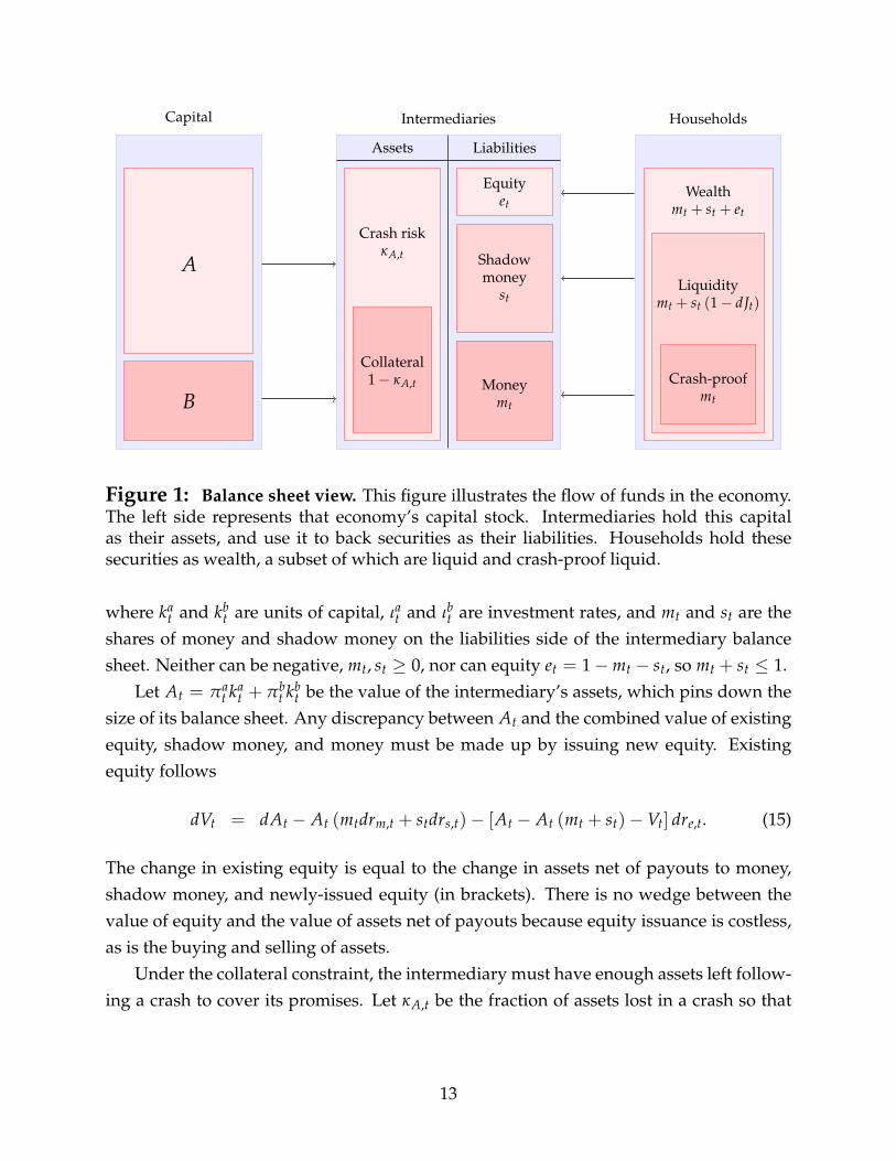
Intermediaries buy capital, set investment, and issue securities to maximize discountedprofits. Figure 1 represents the intermediary balance sheet in relation to the rest of theeconomy.

Although we combine the investment and liquidity provision functions under oneroof, these can easily be separated by adding entrepreneurs. We think of the intermedi-aries as financial institutions since they add value by tranching assets.

The environment is perfectly competitive so each intermediary takes prices as given.Moreover, in contrast to the literature, intermediaries are free to issue and repurchaseequity at no cost, so current net worth is not a state variable. This allows us to solve for theintermediary’s optimal capital structure in closed form given prices and their dynamics.

Intermediaries face a collateral constraint that restricts their ability to provide liquid-ity. Specifically, all claims must be secured by their assets.19 We further restrict attentionto securities whose payoff is nondecreasing in asset value, a natural and commonplace re-striction.20 In Section 3.2 we show that under these conditions crash-proof liquid money,liquid shadow money, and illiquid equity as in (10)–(12) implement the solution to theintermediaries’ optimization problem.

Each intermediary maximizes the value of its existing equity Vt, which is discountedat the equilibrium equity rate of return:

µe,tVtdt = maxka

t ,kbt ,ιat ,ιbt ,mt,st

[(γa − ιat

)ka

t +(

γb − ιbt

)kb

t

]dt + Et [dVt] , (14)

19A collateral constraint can be microfounded with lack of commitment. Payments not explicitly backedby assets are not optimal ex post as there are no reputation or distress costs of reneging on a promise.

20See Innes (1990), Nachman and Noe (1994), DeMarzo and Duffie (1999), and DeMarzo (2005) for usesand justifications for such a restriction.

12

Capital Intermediaries Households

Assets Liabilities

A

B

Crash riskκA,t

Collateral1− κA,t Money

mt

Shadowmoney

st

Equityet

Wealthmt + st + et

Liquiditymt + st (1− dJt)

Crash-proofmt

Figure 1: Balance sheet view. This figure illustrates the flow of funds in the economy.The left side represents that economy’s capital stock. Intermediaries hold this capitalas their assets, and use it to back securities as their liabilities. Households hold thesesecurities as wealth, a subset of which are liquid and crash-proof liquid.

where kat and kb

t are units of capital, ιat and ιbt are investment rates, and mt and st are theshares of money and shadow money on the liabilities side of the intermediary balancesheet. Neither can be negative, mt, st ≥ 0, nor can equity et = 1−mt − st, so mt + st ≤ 1.

Let At = πat ka

t + πbt kb

t be the value of the intermediary’s assets, which pins down thesize of its balance sheet. Any discrepancy between At and the combined value of existingequity, shadow money, and money must be made up by issuing new equity. Existingequity follows

dVt = dAt − At (mtdrm,t + stdrs,t)− [At − At (mt + st)−Vt] dre,t. (15)

The change in existing equity is equal to the change in assets net of payouts to money,shadow money, and newly-issued equity (in brackets). There is no wedge between thevalue of equity and the value of assets net of payouts because equity issuance is costless,as is the buying and selling of assets.

Under the collateral constraint, the intermediary must have enough assets left follow-ing a crash to cover its promises. Let κA,t be the fraction of assets lost in a crash so that

13

1− κA,t is the available asset collateral. We then have

mt + st (1− κs,t) ≤ 1− κA,t. (16)

Each dollar of collateral can back one dollar of money and 1/ (1− κs,t) dollars of shadowmoney. This makes it cheaper for the intermediary to deliver normal-times liquidity evenas households prefer crash-proof liquidity, a key tradeoff.

3 Analysis

In this section we present analytical results that characterize households’ demand forliquidity and intermediaries’ supply of liquidity given asset prices and their dynamics.Results for the full equilibrium are in Section 4 below.

3.1 The demand for liquidity

Households use liquid securities to self-insure against liquidity events. Abundant liquid-ity encourages saving and drives down discount rates. As crashes become more likely,demand for money, which is crash-proof liquid rises and demand for shadow money falls.

The household problem (4) can be written as the Hamilton-Jacobi-Bellman equation

ρVht = max

ct,Ct,mt,stWt

(ctdt + ψEt

[CtdNh

t

])+ Et

[dVh

t

], (17)

where mt and st are portfolio holdings in money and shadow money. The budget dynam-ics and liquidity constraints are

dWt

Wt= −ctdt− CtdNh

t + dre,t + mt (drm,t − dre,t) + st (drs,t − dre,t) (18)

Ct ≤ min{

Ct, lt}

(19)

lt = mt + st (1− dJt) . (20)

Constraint (19) says that liquidity-event consumption must be financed by liquid bal-ances. It always binds since ψ > 1. Equation (20) defines those liquid balances, capturingthe fact that shadow money ceases to be liquid in a crash.

Risk neutrality gives Vht = Wt. Outside a liquidity event, consumption is elastic.21

21This is a standard feature of risk-neutral preferences and it implies that consumption can be negative.Note that even though liquidity-event consumption is lumpy, non-liquidity-event consumption is of order

14

The portfolio optimality conditions are

µe,t − µm,t = h (ψ− 1)[e−τλt e−η(mt+st) +

(1− e−τλt

)e−ηmt

](21)

µs,t − µm,t = h (ψ− 1)(

1− e−τλt)

e−ηmt . (22)

The calculations are in Appendix C. Equity pays a premium over shadow money, andshadow money a premium over money. The total equity premium equals the marginalvalue of liquidity in all states. The premium of shadow-money over money, which wecall the safety premium, equals the marginal value of liquidity in a crash. It is increasingin the level of uncertainty λt.

Evaluating the HJB equation at the optimum gives the total return on savings, whichequals the aggregate cost of capital in equilibrium,

ρ− hη(ψ− 1) +

hη(ψ− 1)

[e−τλt e−η(mt+st) +

(1− e−τλt

)e−ηmt

]. (23)

The cost of capital is decreasing in the supply of liquidity. Greater liquidity promotessaving by raising the opportunity for consumption during a liquidity event when it ismost valuable.

3.2 The supply of liquidity

The intermediary problem consists of the HJB equation (14) subject to the equity dynamics(15), the collateral constraint (16), and the non-negativity constraints mt, st, et ≥ 0. In thissection we focus on the liabilities side of this problem.

Although there are no differences in expertise or preferences between households andintermediaries, holding capital without intermediation is not efficient in this economy. Inall regions of the state-space, at least two of the three available securities are required foroptimal liquidity provision, as we show below. Tranching is always efficient, and this ishow intermediaries add value.

In Appendix C, we state the intermediary’s problem more generally as a security de-sign problem subject to the information sensitivity constraints imposed by Definition 1.This allows us to show rather than assume that crash-proof liquid money, liquid shadowmoney, and illiquid equity as in (10)–(12) are optimal. We state the end result here asfollows:

dt since non-liquidity-event marginal utility is constant at one.

15

κ

mt

mt + st

1− κA,t

1−κA,t1−κ

1− κA,t

(ii)

(iii)

(iv)

0

Figure 2: Optimal capital structure. This figure illustrates cases (ii)–(iv) in Proposi-tion 1. The horizontal axis plots crash-proof liquidity mt and the vertical axis plots totalliquidity mt + st. Note the horizontal axis crosses at 1− κA,t. The blue line represents thecollateral constraint of the intermediary. The red lines represent household indifferencecurves.

Proposition 1. Let κA,t > 0 and σA,t > 0 be the crash risk and normal-times risk exposuresof an intermediary’s balance sheet. Then the intermediary’s optimal capital structure policy canbe implemented with crash-proof liquid money mt, liquid shadow money st (with κs,t = κ), andilliquid equity et = 1−mt − st (with κe,t = 1) as follows:

i. mt = 1− κA,tκ and st =

κA,tκ if κA,t ≤ κ and κA,t <

κη log

(κ

1−κe−τλt

1−e−τλt

);

ii. mt = 0 and st =1−κA,t

1−κ if κA,t > κ and κA,t > 1− 1−κη log

(κ

1−κe−τλt

1−e−τλt

);

iii. mt = 1− κA,t and st = 0 if λt > − 1τ log (1− κ) and κA,t > e; and

iv. mt = 1− κA,t − 1−κη log

(κ

1−κe−τλt

1−e−τλt

)and st =

1η log

(κ

1−κe−τλt

1−e−τλt

)otherwise.

Proof. The proof is contained in Appendix C.

Case (i) of Proposition 1 corresponds to very low asset risk κA,t and uncertainty λt,allowing intermediaries to reduce equity to a minimum. Figure 2 illustrates the intuitionof cases (ii)–(iv). It plots the supply of total liquidity in the form of money and shadowmoney issuance mt + st against crash-proof liquidity mt. The blue line represents theintermediary’s liquidity provision budget, which is pinned down by available collateral

16

1− κA,t. Changes in collateral thus shift the feasibility frontier, expanding and contractingthe total supply of liquidity.

The red lines in Figure 2 depict household demand, which shifts the composition ofliquidity. The indifference curves are defined over crash-proof liquidity and total liquid-ity, as implied by the first-order conditions (21) and (22). Their slope depends on un-certainty λt which determines household willingness to substitute between normal-timesand crash-proof liquidity.

When λt is sufficiently low, we get case (ii) in which shadow money completelycrowds out money and no crash-proof liquidity is produced. As λt rises, the marginalrate of substitution between normal-times and crash-proof liquidity falls so that in case(iv) it is equated to the marginal rate of transformation coming from the intermediarycollateral constraint. Then in case (iii) high uncertainty pushes intermediaries to a cornersolution in which shadow banking shuts down.

Proposition 1 shows that the optimal provision of liquidity generally requires shadowbanking. The sole exception is case (iii). The rest of the time, shadow banking allows thefinancial sector to increase the supply of liquidity by levering up limited collateral. At thesame time, the liquidity it provides is fragile: it disappears when uncertainty rises.

We also see that equity takes all normal-times risk σA,t. This is optimal because if aliquid security had a positive normal-times risk exposure, it would require additional col-lateral in order to remain informationally insensitive and hence liquid ex ante. Residualrisk makes equity an inefficient security for providing liquidity.

As Figure 2 shows, an intermediary’s ability to issue liquid securities is constrainedby the collateral value of its assets (see (16)). Applying Ito’s Lemma to assets At andtaking the crash-risk component, this collateral value is

1− κA,t =πa

t kat

πat ka

t + πbt kb

t

(1− κa

)(1− κa

π,t

)+

πbt kb

t

πat ka

t + πbt kb

t

(1− κb

) (1− κb

π,t

). (24)

The collateral value of assets is a value-weighted average of the collateral value of eachtype of asset on the intermediary’s balance sheet. In turn, the collateral value of eachtype of asset depends on the exposure of its cash flows (κa and κb) and its price (κa

π,t andκb

π,t) to crash risk. The model thus features both exogenous and endogenous risk. Evena cash-flow safe asset (e.g. κb = 0) cannot in general back money directly, as fluctuationsin liquidity premia inject risk into its price (σb

π,t, κbπ,t > 0). The liquidity services that an

asset can support thus become an important component of its value.We turn to the intermediaries’ asset choice in the following section.

17

3.3 Asset prices and investment

On the asset side of their balance sheet, intermediaries purchase capital and set invest-ment. The optimality conditions of the intermediary problem with respect to capital pindown asset prices:

πit =

γi − ιit[µe,t − θ1,t

(1− κi

) (1− κi

π,t

)− θ2,t

]−[µi

π,t + κiκiπ,tλt + φ

(ιit)− δ] (25)

for i = a, b, where θ1,t and θ2,t are the Lagrange multipliers on the collateral and equitynon-negativity constraints. The derivation is in Appendix C.

Prices have the familiar form of current net cash flows over a discount rate minus agrowth rate. The net cash flow, output minus investment, tends to be higher for A capitalsince γa > γb. The growth rate (second bracketed term in the denominator) consists ofprice growth, physical growth, and depreciation.

The first bracketed term in the denominator of (25) is the discount rate. It variesacross the two assets as a result of their differential ability to back liquidity provision.Both assets are funded at a discount from the cost of equity, and this discount dependson their collateral values. Since A capital is riskier, κa > κb, and since collateral is scarce,θ1,t > 0, A’s discount rate tends to be higher than B’s. Although it has higher cash flows,A can have a lower price than B if liquidity is sufficiently scarce. As liquidity becomesmore abundant and the overall cost of capital falls, the wedge in discount rates betweenthe two types of capital shrinks.

The optimal investment policy follows standard q-theory:

1 = πitφ′(

ιit

)(26)

for i = a, b. Since φ is concave, investment is increasing in asset prices. As liquidity affectsdiscount rates and prices, it also affects investment, both overall and across assets.

Taking prices as given and setting investment accordingly, intermediaries shape theevolution of the economy’s capital mix. This capital mix is slow-moving due to tech-nological illiquidity (convex adjustment costs). It can be summarized by the A-capitalshare χt = ka

t /(ka

t + kbt), which becomes a second state variable (after λt). Applying Ito’s

18

Lemma and substituting (1), the dynamics of χt are

dχt = µ (1− 2χt) dt + χt (1− χt)[φ(

ιat

)− φ

(ιbt

)+ λt

(κa − κb

)]dt (27)

−χt (1− χt)

[κa − κb

χt (1− κa) + (1− χt)(1− κb

)] dJt.

In a crash, χt falls as more of the risky capital is wiped out. Crashes thus shift theeconomy’s capital stock towards safety, which produces a dampening effect; uncertaintyshocks absent a crash have a stronger impact on asset prices.22

Absent a crash, the risky capital share drifts according to relative investment in thetwo technologies, φ

(ιat

)− φ

(ιbt

)(the remaining terms of (27) consists of a level-inflow

and crash-compensating terms). This means that in low-uncertainty states when liquidityis abundant so discount rates and collateral premia are low, the economy tends to drifttowards a riskier capital mix. Conversely, the same force pushes towards retrenchment atthe expense of future growth when liquidity provision contracts following a crash.

The model thus features endogenous buildups of economic fragility during boomsand slow recoveries following crashes. Both are dynamic effects resulting from variationin the level and cross-sectional dispersion of discount rates induced by the expansion andcontraction of liquidity provision through shadow banking.

4 Results

In this section, we present results for the full dynamic equilibrium of the model, focusingon the interaction between the macroeconomy and financial markets. We solve for pricesπa (λt, χt) and πb (λt, χt) using projection methods, specifically Chebyshev collocation.Appendix D provides details.

We follow Brunnermeier and Sannikov (2014b) and pick an investment cost functionthat implies quadratic adjustment costs, φ (ιt) =

1ϕ

(√1 + 2ϕιt − 1

). Our benchmark pa-

rameter values are available in Table 1. We view these as an illustration rather than acalibration.

Table 1 about here.22There are several ways to remove the dampening effect: (1) introduce a capital composition shock

that converts some fraction of the safe capital into risky capital when a crash hits; and (2) a crash neednot destroy any capital in the aggregate, it is enough that it destroy some units of capital while benefitingothers (a dispersion shock) as long as investors cannot hold fully diversified portfolios. We pursue the latterapproach in Sections 4.4 (Flight to quality) and 5.2 (Operation Twist).

19

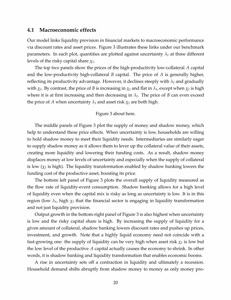
4.1 Macroeconomic effects

Our model links liquidity provision in financial markets to macroeconomic performancevia discount rates and asset prices. Figure 3 illustrates these links under our benchmarkparameters. In each plot, quantities are plotted against uncertainty λt at three differentlevels of the risky capital share χt.

The top two panels show the prices of the high-productivity low-collateral A capitaland the low-productivity high-collateral B capital. The price of A is generally higher,reflecting its productivity advantage. However, it declines steeply with λt and graduallywith χt. By contrast, the price of B is increasing in χt and flat in λt, except when χt is highwhere it is at first increasing and then decreasing in λt. The price of B can even exceedthe price of A when uncertainty λt and asset risk χt are both high.

Figure 3 about here.

The middle panels of Figure 3 plot the supply of money and shadow money, whichhelp to understand these price effects. When uncertainty is low, households are willingto hold shadow money to meet their liquidity needs. Intermediaries are similarly eagerto supply shadow money as it allows them to lever up the collateral value of their assets,creating more liquidity and lowering their funding costs. As a result, shadow moneydisplaces money at low levels of uncertainty and especially when the supply of collateralis low (χt is high). The liquidity transformation enabled by shadow banking lowers thefunding cost of the productive asset, boosting its price.

The bottom left panel of Figure 3 plots the overall supply of liquidity measured asthe flow rate of liquidity-event consumption. Shadow banking allows for a high levelof liquidity even when the capital mix is risky as long as uncertainty is low. It is in thisregion (low λt, high χt that the financial sector is engaging in liquidity transformationand not just liquidity provision.

Output growth in the bottom-right panel of Figure 3 is also highest when uncertaintyis low and the risky capital share is high. By increasing the supply of liquidity for agiven amount of collateral, shadow banking lowers discount rates and pushes up prices,investment, and growth. Note that a highly liquid economy need not coincide with afast-growing one: the supply of liquidity can be very high when asset risk χt is low butthe low level of the productive A capital actually causes the economy to shrink. In otherwords, it is shadow banking and liquidity transformation that enables economic booms.

A rise in uncertainty sets off a contraction in liquidity and ultimately a recession.Household demand shifts abruptly from shadow money to money as only money pro-

20

vides crash-proof liquidity. Intermediaries cater to this demand by adjusting their lia-bilities. The shadow banking sector effectively shuts down within a narrow range ofuncertainty. In the financial crisis of 2007 to 2008, the market for asset-backed commercialpaper suffered a similarly rapid collapse (Acharya, Schnabl and Suarez, 2013).

Issuing more money requires raising equity. The result is less liquidity transforma-tion, less liquidity, and higher discount rates. The price of A capital falls sharply whileB capital becomes more valuable as the liquidity shortage increases the premium for col-lateral. This effect is strongest when collateral is scarce to begin with (χt is high) andliquidity transformation is at its peak. The reversal of investment from productive to safecapital can be interpreted as collateral mining or building a “fortress balance sheet”.

Importantly, it is neither a lack of intermediary capital nor a lack of investment op-portunities that causes intermediaries to stop investing in productive capital when un-certainty rises. It is instead the low level of liquidity transformation resulting from thecontraction of shadow banking that initiates the downturn.

4.2 Persistence

Our model features persistence due to learning and variation in investment, which inter-act dynamically to produce cycles. The endogenous dynamics of collateral values nearthe bottom of the cycle play an important role in this process, a discussion we postponeuntil Section 4.3 below.

A rise in uncertainty contracts liquidity provision, which changes the economy’s tar-get capital mix so that productivity growth remains low even after uncertainty recedes, aform of slow recovery following a financial crisis. At the other end, low uncertainty pro-motes the accumulation of risky capital backed by shadow money issuance, which buildsup fragility during booms.

To illustrate these forces, Figure 4 plots impulse response functions for the state vari-ables uncertainty, λt, and the risky capital share, χt. The plots on the left condition on alow initial level of λt and those on the right on a high one, i.e. a boom versus a bust.

The top panels look at λt. The gray shading represents a contour plot of its conditionaldensity, which is computed by solving the forward Kolmogorov equation in Appendix E.From the solid red lines, which represent conditional means, we see that λt is very persis-tent. From the shaded densities we see that this persistence is due to the combination of anegative drift that pulls much of the mass down and occasional jumps that send chunksof it back up. In this way uncertainty tends to be very low after a long quiet period but itcan rise suddenly as in a “Minsky moment”.

21

Figure 4 about here.

The bottom panels of Figure 4 plot the conditional means of the risky capital share χt

starting from a low, medium, or high level under each of the two λt scenarios. On the left,where λt is low, χt is increasing over time except when it is very high to begin with. Lowuncertainty promotes shadow banking which enables greater liquidity, reducing discountrates and collateral premia. The price of the risky asset rises and stimulates investment.Over time, this leads to a riskier capital mix.

On the right, where λt is high, χt drifts down except when it is very low from the start.When uncertainty is high, households are unwilling to hold shadow money, which makesinvestment in the risky asset less attractive. At the same time, demand for collateralcauses investment in the safe but unproductive asset to pick up (“collateral mining”),causing χt to fall over time. This sets up a slow recovery once uncertainty diminishes.

Overall, Figure 4 illustrates the interaction between the model’s financial and macroe-conomic cycles. In the next section we show how the dynamics of collateral values con-tribute to this interaction.

4.3 Collateral runs

Collateral runs (or margin spirals in the language of Brunnermeier and Pedersen, 2009)are episodes during which liquidity creation requires progressively greater amounts ofcollateral, which is equivalent to a rise in haircuts in financial markets.23

To be concrete, an asset i that can back 1− κ dollars of money per dollar of value has ahaircut of κ. The haircut measures the size of the drop in value that must occur before debtholders take a hit. In our model haircuts have an exogenous cash flow component κi andan endogenous price component κi

π, i = a, b for an overall haircut of 1−(1− κi) (1− κi

π

).

A collateral run occurs when κiπ = 1− πi

+/πi rises as πi falls (pluses denote after-crashprices). This requires a simultaneous rise in the the level and volatility of discount rates.The higher level puts downward pressure on prices, while the higher volaitlity depressesafter-crash collateral values, increasing haircuts. The resulting tightening in the collateralconstraint further amplifies the initial increase in discount rates, causing a downwardprice spiral.

Figure 5 about here.

23A collateral run is distinct from a classic bank run. Agents in our model demand bigger haircuts whenfinancial conditions become more sensitive to uncertainty shocks. They do not face a first-come-first-servedconstraint as in Diamond and Dybvig (1983). A bank run could arise in our model if collateral is rehypoth-ecated among investors. We hope to explore this possibility in future research.

22

To demonstrate the effects of collateral runs, Figure 5 compares haircuts, capital struc-tures, funding costs, and asset prices in economies with and without shadow banking.24

We fix χt = 0.5 and look across λt.In a shadow-banking economy near the peak of a boom (low λt), an uptick in uncer-

tainty leads to a rise in both haircuts and discount rates. Higher haircuts drive a sharpcontraction in liquidity transformation, forcing a shift towards more expensive funding.As a result, prices fall further, which represents a collateral run.

In a collateral run, money yields fall while shadow money yields rise sharply. Sincethe economy is near its peak, shadow banking activity is very high and so overall discountrates rise. The risky A capital suffers the greatest price decline as its funding is mostfragile. Although the amplification of collateral runs causes discount rates to spike abovetheir levels in the no-shadow-banking economy, the price of A capital is always higherwith shadow banking than without because prices capitalize the lower funding costs ina shadow banking-driven boom. The possibility of future booms leads to less severedownturns.

On the other side, when λt is high and liquidity transformation is near bottom, assetprices become less sensitive to uncertainty so a rise in λt actually reduces haircuts. Inother words, the haircut-price dynamic reverses so that a “collateral decelerator” even-tually puts a floor under asset prices. The same dynamic means, however, that haircutsinitially rise as uncertainty begins to subside, which slows down the recovery of assetprices. The same mechanism that amplifies downturns also prolongs their aftermath.

4.4 Flight to quality

Our model generates flight to quality, a rise in the value of safe claims even as overallprices fall. A rise in uncertainty triggers a demand shift from shadow money to money,causing the spread between them to open up. As intermediaries absorb the excess de-mand for money, liquidity transformation shuts down. The premium for collateral rises,causing the safe B capital to appreciate relative to the risky A capital. When this relativeprice change dominates the overall rise in discount rates, the yield of money falls and theprice of B capital rises.

Our benchmark parametrization produces strong flight to quality in securities mar-kets and modest flight to quality in asset markets (see Figure 3). Intuitively, flight toquality is the result of a shortage of collateral due to a sharp contraction in liquidity trans-

24We implement an economy with no shadow banking by setting κ = 0, which removes the leverageadvantage of shadow money.

23

formation. In our benchmark model crashes actually increase the supply of collateral asa higher proportion of the safe B capital remains intact. In this section, we modify themodel slightly to remove this dampening, which intensifies flight to quality effects.

Specifically, we transform the aggregate cash flow shock into a dispersion shock. Letka

i,t and kbi,t be the capital holdings of intermediary i and modify equation (1):

dkai,t

kai,t

=[φ(ιai,t)− δ]

dt− κai,tdNt, (28)

where κai,t = ±κa with probability 1/2 each and κb

i,t = 0 for simplicity. We have furthersimplified our benchmark specification by setting µ = 0, which increases the scarcityof collateral at high levels of χt. We also increase η slightly to 2.8, which reduces theelasticity of substitution between money and shadow money.25

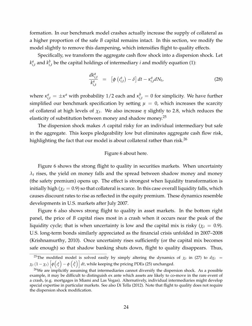
The dispersion shock makes A capital risky for an individual intermediary but safein the aggregate. This keeps pledgeability low but eliminates aggregate cash flow risk,highlighting the fact that our model is about collateral rather than risk.26

Figure 6 about here.

Figure 6 shows the strong flight to quality in securities markets. When uncertaintyλt rises, the yield on money falls and the spread between shadow money and money(the safety premium) opens up. The effect is strongest when liquidity transformation isinitially high (χt = 0.9) so that collateral is scarce. In this case overall liquidity falls, whichcauses discount rates to rise as reflected in the equity premium. These dynamics resembledevelopments in U.S. markets after July 2007.

Figure 6 also shows strong flight to quality in asset markets. In the bottom rightpanel, the price of B capital rises most in a crash when it occurs near the peak of theliquidity cycle; that is when uncertainty is low and the capital mix is risky (χt = 0.9).U.S. long-term bonds similarly appreciated as the financial crisis unfolded in 2007–2008(Krishnamurthy, 2010). Once uncertainty rises sufficiently (or the capital mix becomessafe enough) so that shadow banking shuts down, flight to quality disappears. Thus,

25The modified model is solved easily by simply altering the dynamics of χt in (27) to dχt =

χt (1− χt)[φ(

ιat

)− φ

(ιbt

)]dt, while keeping the pricing PDEs (25) unchanged.

26We are implicitly assuming that intermediaries cannot diversify the dispersion shock. As a possibleexample, it may be difficult to distinguish ex ante which assets are likely to co-move in the rare event ofa crash, (e.g. mortgages in Miami and Las Vegas). Alternatively, individual intermediaries might developspecial expertise in particular markets. See also Di Tella (2012). Note that flight to quality does not requirethe dispersion shock modification.

24

flight to quality results from the acute shortage of collateral that occurs when uncertaintyrises suddenly after a shadow banking boom.

Our model’s learning dynamics tie together normal-times (dB) and crash (dN) flightto quality (both raise λ). The two, however, are conceptually distinct as normal-timesshocks are borne entirely by equity whereas crashes affect collateral values and the supplyof liquidity. In our model only crash-driven flight to quality is important ex ante becauseequity markets are frictionless.27 This observation suggests that differences in the pricingof instruments that act as normal-times versus crash-risk hedges can be used to assess theimportance of equity- versus collateral-based frictions.

5 Policy interventions

In the aftermath of the 2008 financial crisis, central banks around the world and the U.S.Federal Reserve in particular have resorted to a wide variety of interventions, broadlyreferred to as unconventional monetary policy. We consider two of these interventions,the Large Scale Asset Purchase (LSAP) program of 2008–2010 and the Maturity ExtensionProgram also known as “Operation Twist” of 2011–2012. Under LSAP, the FED purchasedlarge amounts of mortgage-backed securities in an effort to support their prices.28 UnderOperation Twist, the FED purchased long-dated Treasurys and sold short-dated ones withthe stated goal of reducing long-term interest rates.29

Alongside central banks, regulators have entertained a broad range of proposals andimplemented a subset of them. We look at two of these, the so-called “Volcker rule”which seeks to separate commercial banking and proprietary trading, and liquidity re-quirements as have been adopted by the Basel III Committee.30

Our aim in this section is to shed light on the interaction of these policies with the

27We explore the policy implications of flight to quality in Section 5.2 (Operation Twist) and Section 5.4(Volcker rule).

28The press release announcing the program reads, “Spreads of rates on GSE debt and on GSE-guaranteedmortgages have widened appreciably of late. This action is being taken to reduce the cost and increase theavailability of credit for the purchase of houses, which in turn should support housing markets and fosterimproved conditions in financial markets more generally” (Federal Open Market Committee, 2008).

29The program’s announcement following the September 2011 FOMC meeting reads, “The Committeeintends to purchase, by the end of June 2012, $400 billion of Treasury securities with remaining maturitiesof 6 years to 30 years and to sell an equal amount of Treasury securities with remaining maturities of 3 yearsor less. This program should put downward pressure on longer-term interest rates and help make broaderfinancial conditions more accommodative” (Federal Open Market Committee, 2011).

30The Basel III framework consists of two parts, the Liquidity Coverage Ratio (LCR), and the Net StableFunding Ratio (NSFR) (Bank for International Settlements, 2010). LCR affects asset liquidity and NSFRaffects liquidity provision directly. From the point of view of the model, what matters is their combinedeffect on liquidity transformation.

25

liquidity transformation channel that lies at the heart of the paper. We leave a compre-hensive welfare analysis that incorporates a broader set of considerations for future work.

5.1 Asset purchases

We interpret LSAP as replacing risky A capital with safe B capital. The direct effect is toincrease the amount of collateral available on intermediary balance sheets, and by exten-sion liquidity provision, asset prices, and investment. Since ex post prices determine exante collateral values, LSAP also has an indirect ex ante effect.

In an LSAP, a given dollar amount of A capital is exchanged for an equal dollaramount of B capital. Any cash flow mismatch between the swapped assets is backedby lump-sump taxation of households (the government does not face a collateral con-straint). We model LSAP as a one-at-a-time intervention to acknowledge the limits of thistaxation power. The model is non-Ricardian because collateral impacts asset prices.

We assume LSAP takes effect with a given probability immediately following a crash(when it is most needed) and it is eventually withdrawn at a given intensity. This setupintroduces a simple binary state variable that corresponds to the state of the central bank’sbalance sheet (empty or full). Appendix F has the details.

Figure 7 implements an LSAP that reduces the risky capital share χt by 0.2. It getstriggered with 50% probability after a crash and is expected to last ten years.

Figure 7 about here.

The top panels of Figure 7 show that in most of the state-space, LSAP pushes the priceof risky capital up and the price of safe capital down, with the effects for both assets beingstrongest when the capital mix is risky (χt = 0.9). In this region, collateral is scarce andliquidity is low. By supplying safe assets, the central bank increases the collateral value ofintermediary balance sheets, allowing for greater liquidity provision. The result is botha decline in overall discount rates which tends to push all prices up, and a decline in thecollateral premium, which pushes the price of risky capital up and the price of safe capitaldown. The net effect is positive for the risky asset and negative for the safe asset.

Interestingly, enacting a program when liquidity is abundant (when χt and λt are low)backfires and actually reduces the price of the risky asset. This is a result of the centralbank’s limited capacity. The economy becomes riskier because the central bank will likelybe out of ammunition at the next crash.

Looking along the λt dimension, the price effects are strongest when uncertainty ismoderately high. This is also the region where collateral runs push haircuts to their high-

26

est levels (see Section 4.3). Thus, LSAP is most effective when the shadow banking sectoris maximally stressed and contracting precipitously.

The middle two panels of Figure 7 consider the ex ante effect of LSAP by comparingprices across economies with and without the possibility of an LSAP intervention. Riskycapital prices are higher and safe capital prices are lower in the LSAP economy through-out the state-space, as expected. Importantly, the ex ante effects are stronger than the expost effects in the low uncertainty region. LSAP has a stabilizing effect ex post when un-certainty is high, which means it boosts collateral values ex ante when uncertainty is low.In this way, expectation of future LSAP interventions amplifies shadow banking booms.This mechanism echoes concerns raised by Rajan (2005).

Finally, we consider the effect of an announcement that policy accommodation will bewithdrawn sooner than anticipated.31 In the lower panels of Figure 7 we show that “tapertalk” produces sharp asset price movements in our model as in the data. Expectationsof premature policy withdrawal can undermine the effectiveness of an asset purchaseprogram.

Our results show that when liquidity transformation is impaired by high uncertainty,an LSAP intervention allows the central bank to support asset prices via collateral trans-formation.

5.2 Operation Twist

We model Operation Twist as a market intervention that reduces the duration of safeassets on intermediary balance sheets. Interestingly, in our framework this can reducepledgeability as long-term safe capital acts as a crash-hedge due to flight to quality. Todemonstrate this effect, we use the parameters from Section 4.4 on flight to quality.

We map the safe asset to government debt by assuming that the private sector cannotcreate it but that the government issues it by following the same policy that intermediariesdo in the benchmark economy (set Tobin’s q to one as in (26)). To model a change induration within an economy, we introduce two types of government debt, zero-durationfloating-rate debt and long-term fixed coupon bonds. Floating debt pays the floating rateµm (the yield of money) and trades at par. Long bonds pay the fixed coupon γb as in thebaseline model. The central bank sets the shares of the two types of bonds as a policyvariable. Details are in Appendix F.

In an Operation Twist intervention, the central bank buys long-term bonds and sells

31In the summer of 2013, discussion of policy withdrawal, or “taper talk”, led to sharp corrections acrossasset markets.

27

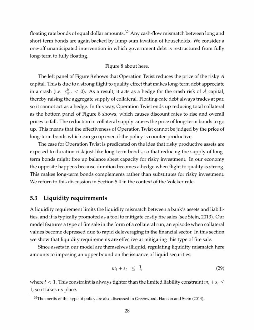
floating rate bonds of equal dollar amounts.32 Any cash-flow mismatch between long andshort-term bonds are again backed by lump-sum taxation of households. We consider aone-off unanticipated intervention in which government debt is restructured from fullylong-term to fully floating.

Figure 8 about here.

The left panel of Figure 8 shows that Operation Twist reduces the price of the risky Acapital. This is due to a strong flight to quality effect that makes long-term debt appreciatein a crash (i.e. κb

π,t < 0). As a result, it acts as a hedge for the crash risk of A capital,thereby raising the aggregate supply of collateral. Floating-rate debt always trades at par,so it cannot act as a hedge. In this way, Operation Twist ends up reducing total collateralas the bottom panel of Figure 8 shows, which causes discount rates to rise and overallprices to fall. The reduction in collateral supply causes the price of long-term bonds to goup. This means that the effectiveness of Operation Twist cannot be judged by the price oflong-term bonds which can go up even if the policy is counter-productive.

The case for Operation Twist is predicated on the idea that risky productive assets areexposed to duration risk just like long-term bonds, so that reducing the supply of long-term bonds might free up balance sheet capacity for risky investment. In our economythe opposite happens because duration becomes a hedge when flight to quality is strong.This makes long-term bonds complements rather than substitutes for risky investment.We return to this discussion in Section 5.4 in the context of the Volcker rule.

5.3 Liquidity requirements

A liquidity requirement limits the liquidity mismatch between a bank’s assets and liabili-ties, and it is typically promoted as a tool to mitigate costly fire sales (see Stein, 2013). Ourmodel features a type of fire sale in the form of a collateral run, an episode when collateralvalues become depressed due to rapid deleveraging in the financial sector. In this sectionwe show that liquidity requirements are effective at mitigating this type of fire sale.

Since assets in our model are themselves illiquid, regulating liquidity mismatch hereamounts to imposing an upper bound on the issuance of liquid securities:

mt + st ≤ l, (29)

where l < 1. This constraint is always tighter than the limited liability constraint mt + st ≤1, so it takes its place.

32The merits of this type of policy are also discussed in Greenwood, Hanson and Stein (2014).

28

Solving the model with a liquidity requirement involves an additional case in theintermediary’s optimal capital structure policy. The specifics are in Appendix F.

Figure 9 about here.

Figure 9 compares an economy with a 10% liquidity requirement (1− l = 10%) to thebenchmark case of a zero liquidity requirement. We fix χt = 0.5 and look across λt.

From the top two panels, we see that the liquidity requirement leads to a drastic re-duction in shadow money issuance. The reason is that the cap on liquidity provisioncurtails the principal advantage of shadow money, the ability to create liquidity with lesscollateral. In fact, money issuance rises as it is no longer crowded out by shadow moneyduring booms.

The middle two panels plot prices, which are lower in the economy with a liquidityrequirement due to lower liquidity provision. Note that this happens even at high uncer-tainty when the liquidity requirement is not binding. The reason is that it is expected tobind when uncertainty is low. In this way taming the boom deepens the bust.

The bottom panels look at haircuts (recall from Section 4.3 that an asset’s haircut isone minus its collateral value). We see that the haircuts of both assets fall, though asset Ahas a much larger haircut to begin with due to greater risk.33

The intuition for this result is that by restraining shadow banking in booms, liquid-ity requirements reduce the economy’s exposure to uncertainty shocks. This means thatprices do not fall as fast when uncertainty rises, so collateral values remain relatively highand haircuts low.

Recall that a collateral run is an event where haircuts rise as prices fall and the tworeinforce each other (Section 4.3). Figure 9 shows that liquidity requirements can indeedarrest this dynamic by slowing the rise in haircuts. This suggests they can be used topromote financial stability.

5.4 The Volcker rule

The Volcker rule seeks to prevent banks from engaging in proprietary trading due to highlevels of risk. Observers have argued that the distinction between market making andproprietary trading is extremely difficult as market making typically involves holding asubstantial inventory of risky assets.

In this section we map market making activity and its associated inventory accumula-tion into holdings of risky capital and interpret the Volcker rule as imposing a segregation

33By fixing χt = 0.5, we are looking at a region with enough collateral where flight to quality does nottake place.

29

between intermediaries that hold risky and safe assets.34 At this level, our analysis couldalso refer to the reintroduction of the Glass-Steagall act, which banned affiliations be-tween commercial banks and securities firms. Once again, our scope here is limited to theliquidity transformation channel.

The key point is that our model features a complementarity between risky and safeasset holdings whenever flight to quality effects are present. The intuition is the same as inthe discussion of Operation Twist in Section 5.2: Flight to quality turns safe capital into ahedge for risky capital on intermediary balance sheets, which raises the overall collateralvalue of intermediary assets. Under a Volcker rule, collateral is effectively wasted as safebanks have too much and risky banks too little.

To illustrate, suppose there is flight to quality so that the value of safe capital risesin a crash (e.g. κb = 0, κb

π,t < 0). Consider a Volcker rule economy with two (types of)intermediaries, a risky-asset bank i = a and a safe-asset bank i = b. Each bank’s balancesheet must satisfy limited liability and the collateral constraint while holding only onetype of capital:

mi + si ≤ min{

1,(

1− κiπ

) (1− κi

)+ siκ

}. (30)

Flight to quality implies that the safe bank has excess collateral that allows it to issue 100%money, mb = 1 and sb = 0. The risky bank behaves as in our model, so its crash-solvencyconstraint binds, ma + sa = (1− κa

π) (1− κa) + saκ. Let x be the value-weighted share ofA capital. Then total liquidity under the Volcker rule and the benchmark economy is

ma + sa + mb + sb = x (1− κaπ) (1− κa) + (1− x) + saκ (31)

m + s = x (1− κaπ) (1− κa) + (1− x)

(1− κb

π

) (1− κb

)+ sκ. (32)

Comparing (31) and (32) it is clear that flight to quality,(1− κb

π

) (1− κb) > 1, leads

to lower liquidity provision in the Volcker economy. In general both normal-times andcrash-proof liquidity are lower even though the Volcker rule only tightens the collateralconstraint coming from crash risk. The scarcity of collateral on the risky bank’s balancesheet reduces its capacity to provide normal-times liquidity with shadow money. At thesame time, the excess collateral on the safe bank’s balance sheet goes unused.

34Note that liabilities-side segregation (e.g. between issuers of money and shadow money) has no effectin our model as the ability to issue equity costlessly allows capital to flow freely across intermediaries.

30

6 Conclusion

We present a model that joins the macroeconomic cycle to the liquidity transformationcycle in the financial sector. The key friction is that while liquidity is valuable, it requirescollateral. Since collateral is particularly scarce after large shocks (crashes), intermediariesoptimally produce state-contingent liquidity in the form of securities that are money-likein normal times but cease to be liquid in a crash. This allows them to produce liquidsecurities from risky assets, that is to engage in liquidity transformation. We call thisprocess shadow banking.

Shadow banking creates booms in which liquidity provision expands, discount ratesfall, asset prices and investment rise, and output grows. At the same time, it buildsfragility by raising the economy’s exposure to uncertainty shocks. Such shocks unleashsevere effects when preceded by a boom: shadow banking disappears and liquidity con-tracts sharply, prices of risky assets fall, amplified by collateral runs, and prices of safeassets rise through flight to quality; investment and growth fall. Recoveries are slow dueto fortress balance sheets and a “collateral decelerator” under which haircuts rise as re-vived liquidity transformation once again restores uncertainty exposure.

In sum, shadow banking enables high levels of liquidity in good times at the expenseof bad times. As it expands and contracts, shadow banking activity shifts the balancebetween financial stability and growth.

31

References

Acharya, Viral, Philipp Schnabl, and Gustavo Suarez. 2013. “Securitization without risktransfer.” Journal of Financial Economics, 107(3): 515–536.

Adrian, Tobias, and Hyun Song Shin. 2009. “Money, Liquidity, and Monetary Policy.”The American Economic Review, 99(2): pp. 600–605.

Adrian, Tobias, and Hyun Song Shin. 2010. “Liquidity and leverage.” Journal of FinancialIntermediation, 19(3): 418–437.

Adrian, Tobias, and Nina Boyarchenko. 2012. “Intermediary leverage cycles and finan-cial stability.” Working paper.

Adrian, Tobias, Emanuel Moench, and Hyun Song Shin. 2010. “Financial intermedia-tion, asset prices, and macroeconomic dynamics.” Federal Reserve Bank of New York StaffReport, 422.

Adrian, Tobias, Erkko Etula, and Tyler Muir. 2014. “Financial Intermediaries and theCross-Section of Asset Returns.” The Journal of Finance, doi: 10.1111/jofi.12189.

Ang, Andrew, Sergiy Gorovyy, and Gregory B. van Inwegen. 2011. “Hedge fund lever-age.” Journal of Financial Economics, 102(1): 102–126.

Ashcraft, Adam, Nicolae Gârleanu, and Lasse Heje Pedersen. 2011. “Two monetarytools: Interest rates and haircuts.” In NBER Macroeconomics Annual 2010, Volume 25.143–180. University of Chicago Press.

Bai, Jennie, Arvind Krishnamurthy, and Charles-Henri Weymuller. 2013. “Measuringthe liquidity mismatch in the banking sector.” Working paper.

Bank for International Settlements. 2010. Basel III: International framework for liquidity riskmeasurement, standards and monitoring.

Bansal, Ravi, Wilbur Coleman, and Christian Lundblad. 2010. “Endogenous LiquiditySupply.” Working paper.

Baron, Matthew, and Wei Xiong. 2014. “Credit Expansion and Neglected Crash Risk.”Working paper.

Bernanke, Ben S. 2013. “Monitoring the Financial System.” At the 49th Annual Confer-ence on Bank Structure and Competition sponsored by the Federal Reserve Bank ofChicago, Chicago, Illinois.

Bernanke, Ben S, and Mark Gertler. 1989. “Agency costs, net worth, and business fluc-tuations.” The American Economic Review, 14–31.

Bernanke, Ben S, Mark Gertler, and Simon Gilchrist. 1999. “The financial accelerator ina quantitative business cycle framework.” Handbook of macroeconomics, 1: 1341–1393.

Bigio, Saki. 2013. “Endogenous liquidity and the business cycle.” Working paper.Brunnermeier, Markus K, and Lasse Heje Pedersen. 2009. “Market liquidity and funding

liquidity.” Review of Financial studies, 22(6): 2201–2238.Brunnermeier, Markus K, and Yuliy Sannikov. 2014a. “The I Theory of Money.” Working

paper.Brunnermeier, Markus K, and Yuliy Sannikov. 2014b. “A macroeconomic model with a

financial sector.” The American Economic Review, 104(2): 379–421.Brunnermeier, Markus K, Thomas Eisenbach, and Yuliy Sannikov. 2013. “Macroeco-

nomics with Financial Frictions: A Survey.” Advances in Economics and Econometrics,Tenth World Congress of the Econometric Society. New York:Cambridge University Press.

Caballero, Ricardo J, and Emmanuel Farhi. 2013. “A Model of the Safe Asset Mechanism(SAM): Safety Traps and Economic Policy.” NBER working paper.

Dang, Tri Vi, Gary Gorton, and Bengt Holmström. 2012. “Financial crises and the opti-mality of debt for liquidity provision.” Working paper.

DeMarzo, Peter, and Darrell Duffie. 1999. “A liquidity-based model of security design.”Econometrica, 67(1): 65–99.

DeMarzo, Peter M. 2005. “The pooling and tranching of securities: A model of informedintermediation.” Review of Financial Studies, 18(1): 1–35.

Diamond, Douglas W, and Philip H Dybvig. 1983. “Bank Runs, Deposit Insurance, andLiquidity.” Journal of Political Economy, 91(3): pp. 401–419.

Di Tella, Sebastian. 2012. “Uncertainty shocks and balance sheet recessions.” Workingpaper.

Drechsler, Itamar, Alexi Savov, and Philipp Schnabl. 2014. “A Model of Monetary Policyand Risk Premia.” Working paper.

Federal Open Market Committee. 2007. “Minutes from the Meeting of the Federal OpenMarket Committee on June 27–28, 2007.” US Federal Reserve.

Federal Open Market Committee. 2008. “Press Release of November 25, 2008.” US FederalReserve.

Federal Open Market Committee. 2011. “Statement following the meeting of the FederalOpen Market Committee on September 11, 2011.” US Federal Reserve.

Financial Crisis Inquiry Commission. 2011. “The Financial Crisis Inquiry Report.” USGovernment Printing Office.

Gârleanu, Nicolae, and Lasse Heje Pedersen. 2011. “Margin-based Asset Pricing andDeviations from the Law of One Price.” Review of Financial Studies.

Gârleanu, Nicolae, Stavros Panageas, and Jianfeng Yu. 2012. “Technological Growth andAsset Pricing.” The Journal of Finance, 67(4): 1265–1292.

Geanakoplos, John. 2003. “Liquidity, Default, and Crashes: Endogenous Contracts inGeneral Equilibrium.” In Advances in Economics and Econometrics. Vol. 2, , ed. MathiasDewatripont, Lars Peter Hansen and Stephen J. Turnovsky, 170–205. Cambridge Uni-versity Press.

Gennaioli, Nicola, Andrei Shleifer, and Robert W. Vishny. 2012. “Neglected risks, fi-nancial innovation, and financial fragility.” Journal of Financial Economics, 104(3): 452 –468. Market Institutions, Financial Market Risks and Financial Crisis.

Gennaioli, Nicola, Andrei Shleifer, and Robert W. Vishny. 2013. “A Model of ShadowBanking.” The Journal of Finance, 68(4): 1331–1363.

Gertler, Mark, and Nobuhiro Kiyotaki. 2010. “Financial Intermediation and Credit Pol-icy in Business Cycle Analysis.” In Handbook of Monetary Economics. Vol. 3 of Handbookof Monetary Economics, , ed. Benjamin M. Friedman and Michael Woodford, Chapter 11,547–599. Elsevier.

Gertler, Mark, and Nobuhiro Kiyotaki. 2013. “Banking, Liquidity and Bank Runs in anInfinite-Horizon Economy.” Working paper.

Gertler, Mark, and Peter Karadi. 2011. “A model of unconventional monetary policy.”Journal of Monetary Economics, 58(1): 17–34.

Gorton, Gary, and Andrew Metrick. 2012. “Securitized banking and the run on repo.”Journal of Financial Economics, 104(3): 425–451.

Gorton, Gary, and George Pennacchi. 1990. “Financial Intermediaries and Liquidity Cre-ation.” The Journal of Finance, 45(1): 49–71.

Gorton, Gary, and Guillermo Ordoñez. 2014. “Collateral crises.” The American EconomicReview, 104(2): 343–378.

Greenwood, Robin, Sam Hanson, and Jeremy Stein. 2014. “A Comparative-AdvantageApproach to Government Debt Maturity.” Journal of Finance, forthcoming.

Hanson, Floyd B. 2007. Applied stochastic processes and control for jump diffusions: Modeling,analysis, and computation. Society for Industrial and Applied Mathematics.

Hanson, Samuel G, Andrei Shleifer, Jeremy C Stein, and Robert W Vishny. 2014.“Banks as Patient Fixed Income Investors.” Working paper.

Harris, Milton, Christian Opp, and Marcus Opp. 2014. “Higher Capital Requirements,Safer Banks? Macroprudential Regulation in a Competitive Financial System.” Workingpaper.

He, Zhigu, and Arvind Krishnamurthy. 2012. “A Model of Capital and Crises.” The Re-view of Economic Studies, 79(2): 735–777.

He, Zhiguo, and Arvind Krishnamurthy. 2013. “Intermediary Asset Pricing.” AmericanEconomic Review, 103(2): 732–770.

He, Zhiguo, and Konstantin Milbradt. 2013. “Endogenous liquidity and defaultablebonds.” Econometrica, forthcoming.

He, Zhiguo, In Gu Khang, and Arvind Krishnamurthy. 2010. “Balance sheet adjustmentsduring the 2008 crisis.” IMF Economic Review, 58(1): 118–156.

Holmström, Bengt, and Jean Tirole. 1998. “Private and Public Supply of Liquidity.” Jour-nal of Political Economy, 106(1): 1–40.

Innes, Robert D. 1990. “Limited liability and incentive contracting with ex-ante actionchoices.” Journal of economic theory, 52(1): 45–67.

Kiyotaki, Nobuhiro, and John Moore. 1997. “Credit Cycles.” Journal of Political Economy,105(2).

Kiyotaki, Nobuhiro, and John Moore. 2012. “Liquidity, business cycles, and monetarypolicy.” Working paper.

Krishnamurthy, Arvind. 2010. “How Debt Markets Have Malfunctioned in the Crisis.”The Journal of Economic Perspectives, 24(1): 3–28.

Krishnamurthy, Arvind, and Annette Vissing-Jorgensen. 2012a. “The aggregate demandfor treasury debt.” Journal of Political Economy, 120(2): 233–267.

Krishnamurthy, Arvind, and Annette Vissing-Jorgensen. 2012b. “Short-term Debt andFinancial Crises: What we can learn from US Treasury Supply.” Working paper.

Krishnamurthy, Arvind, and Annette Vissing-Jorgensen. 2013. “The Ins and Outs ofLSAPs.” 2013 Federal Reserve Bank of Kansas City Economic Policy Symposium, Jackson Hole,Wyoming.

Krishnamurthy, Arvind, Stefan Nagel, and Dmitry Orlov. 2014. “Sizing up repo.” TheJournal of Finance, doi: 10.1111/jofi.12168.

Kurlat, Pablo. 2013. “Lemons Markets and the Transmission of Aggregate Shocks.” Amer-ican Economic Review, 103(4): 1463–1489.

Liptser, Robert S, and Albert N Shiryaev. 2001. Statistics of Random Processes II: II. Appli-cations. Vol. 2, Springer.

Maggiori, Matteo. 2013. “Financial intermediation, international risk sharing, and reserve

currencies.” Working paper.McCauley, Robert, and Patrick McGuire. 2009. “Dollar appreciation in 2008: safe haven,

carry trades, dollar shortage and overhedging.” BIS Quarterly Review.Minsky, Hyman P. 1986. Stabilizing an unstable economy. Yale University Press New Haven,

CT.Nachman, David C, and Thomas H Noe. 1994. “Optimal design of securities under asym-

metric information.” Review of Financial Studies, 7(1): 1–44.Nagel, Stefan. 2014. “The Liquidity Premium of Near-Money Assets.” Working paper.Rajan, Raghuram G. 2005. “Has finance made the world riskier?” 2005 Federal Reserve

Bank of Kansas City Economic Policy Symposium, Jackson Hole, Wyoming.Rampini, Adriano, and S Viswanathan. 2012. “Financial intermediary capital.” Working

paper.Reinhart, Carmen M, and Kenneth Rogoff. 2009. This time is different: Eight centuries of

financial folly. Princeton University Press.Reinhart, Carmen M, and Vincent R Reinhart. 2010. “After the fall.” Working paper.Sannikov, Yuliy. 2013. “Quiet Times and Financial Fragility.” Working paper.Schularick, Moritz, and Alan M Taylor. 2012. “Credit Booms Gone Bust: Monetary

Policy, Leverage Cycles, and Financial Crises, 1870-2008.” American Economic Review,102(2): 1029–61.

Stein, Jeremy. 2013. “The Fire-Sales Problem and Securities Financing Transactions.” Atthe Federal Reserve Bank of New York Workshop on Fire Sales as a Driver of SystemicRisk in Triparty Repo and other Secured Funding Markets, New York, 4 October 2013.

Sunderam, Adi. 2013. “Money Creation and the Shadow Banking System.” Working paper.Wonham, W Murray. 1965. “Some applications of stochastic differential equations to op-

timal nonlinear filtering.” Journal of the Society for Industrial and Applied Mathematics,Series A: Control, 2(3): 347–369.

Table 1: Benchmark parameter values

This table contains the values for the model parameters used forproducing the benchmark results of the paper.

Description Parameter Value

Subjective discounting parameter ρ 0.40Depreciation δ 0.03Level-inflow of capital µ 0.01Adjustment cost parameter ϕ 5Asset A cash flow risk κa 0.4Asset B cash flow risk κb 0.0Asset A productivity γa 0.08Asset B productivity γb 0.03Low uncertainty state λL 0.1High uncertainty state λH 2.1Low uncertainty state exit rate qL 0.05High uncertainty state exit rate qH 0.05Uncertainty news signal precision 1/σ 0.1Liquid asset risk upper bound κ 0.7Liquidity event duration τ 1.032Liquidity event intensity h 0.1Value of liquidity-event consumption ψ 10Average liquidity shock size 1/η 0.5

Figure 3: Prices, issuance, liquidity-event consumption, and growth

This figure plots capital prices, money issuance, shadow money issuance, output growth,and liquidity services using the benchmark parameter values in Table 1. Each quantityis plotted against uncertainty λt while holding the risky capital share χt fixed at a low(0.1), medium (0.5), and high (0.9) level. Growth is the expected growth rate of outputyt = γaka

t + γbkbt . Liquidity-event consumption is the flow rate of Et

[CtdNh

t].

Asset A price (πa) Asset B price (πb)

0.5 1 1.5 20.8

1

1.2

1.4

1.6

λ

0.5 1 1.5 20.8

0.85

0.9

0.95

1

λ

Money (m) Shadow money (s)

0.5 1 1.5 20.2

0.4

0.6

0.8

1

λ

0.5 1 1.5 20

0.2

0.4

0.6

0.8

λ

Liquidity-event consumption Growth

0.5 1 1.5 20.034

0.036

0.038

0.04

0.042

0.044

0.046

λ

0.5 1 1.5 2−0.06

−0.04

−0.02

0

0.02

λ

χ = 0.1 χ = 0.5 χ = 0.9

Figure 4: Persistence

The evolution of uncertainty λt, and the capital mix χt over time starting from a initialcondition of low (left, λ0 = 0.6) or high (right, λ0 = 1.6) levels of λt, and low (χ0 = 0.1),medium (χ0 = 0.5), or high (χ0 = 0.9) levels of χt. The top two panels show the evolutionof λt (which is independent of χt) with solid red lines for the conditional mean of λt,E0 [λt| λ0], and gray shading for the conditional density of λt. The bottom panels showthe conditional means of χt, E0 [χt| λ0, χ0]. The conditional means and densities arecomputed using the forward Kolmogorov equation in Appendix E.

Low initial uncertainty High initial uncertainty

E [λt| λ0 = 0.6] E [λt| λ0 = 1.6]

t

0 1 2 3 4 5

0.5

1

1.5

2

t

0 1 2 3 4 5

0.5

1

1.5

2

E [χt| λ0 = 0.6, χ0] E [χt| λ0 = 1.6, χ0]

t

0 1 2 3 4 50

0.2

0.4

0.6

0.8

1

t

0 1 2 3 4 50

0.2

0.4

0.6

0.8

1

χ0 = 0.1 χ0 = 0.5 χ0 = 0.9

Figure 5: Collateral runs

Equilibrium haircuts, capital structure, funding costs, and prices for economies with(no markers) and without (circle markers) shadow banking. The risky capital share isfixed at χt = 0.5. Haircuts are defined as one minus the collateral value of the asset, i.e.1−

(1− κi) (1− κi

π

)for i = a, b.

Haircuts Capital structure

0.5 1 1.5 20

0.1

0.2

0.3

0.4

0.5

λ

A B Agg.

0.5 1 1.5 20

0.2

0.4

0.6

0.8

1

λ

m s e

Funding costs Prices

0.5 1 1.5 2−0.05

0

0.05

0.1

0.15

0.2

0.25

0.3

λ

µm µ s µ e

0.5 1 1.5 20.7

0.8

0.9

1

1.1

1.2

1.3

1.4

λ

A B

Figure 6: Flight to quality

The yield on money, the spread between shadow money and money (the safety pre-mium), the equity premium, and the crash-return of B capital for the model with adispersion shock κa

i = 0.6 (see discussion in Section 4.4), µ = 0 and η = 2.8.

Money yield (µm) Safety premium (µs − µm)

0.5 1 1.5 2−0.08

−0.06

−0.04

−0.02

0

0.02

λ

0.5 1 1.5 20

0.1

0.2

0.3

0.4

λ

Equity premium (µe − µm) B crash return (πb+/πb − 1)

0.5 1 1.5 20.1

0.2

0.3

0.4

0.5

λ

0.5 1 1.5 20

0.01

0.02

0.03

0.04

0.05

0.06

λ

χ = 0.1 χ = 0.5 χ = 0.9

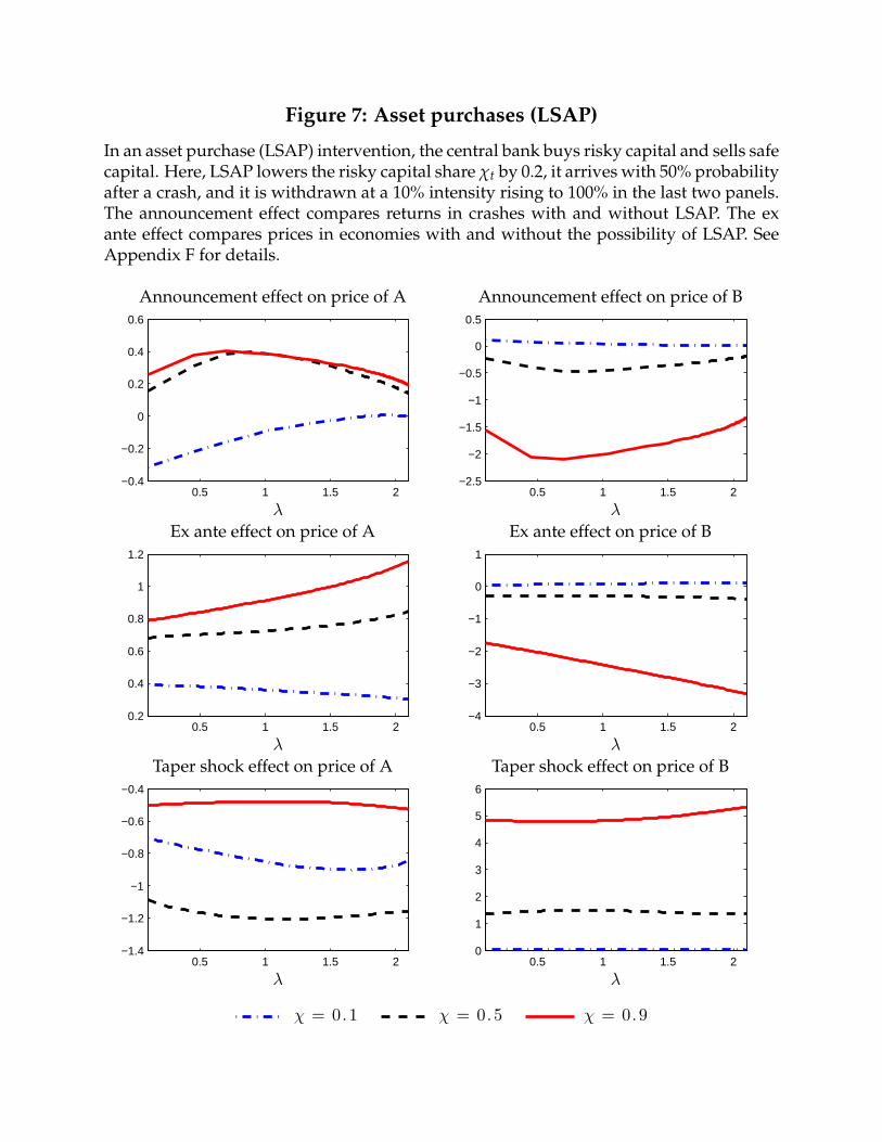
Figure 7: Asset purchases (LSAP)

In an asset purchase (LSAP) intervention, the central bank buys risky capital and sells safecapital. Here, LSAP lowers the risky capital share χt by 0.2, it arrives with 50% probabilityafter a crash, and it is withdrawn at a 10% intensity rising to 100% in the last two panels.The announcement effect compares returns in crashes with and without LSAP. The exante effect compares prices in economies with and without the possibility of LSAP. SeeAppendix F for details.

Announcement effect on price of A Announcement effect on price of B

0.5 1 1.5 2−0.4

−0.2

0

0.2

0.4

0.6

λ0.5 1 1.5 2

−2.5

−2

−1.5

−1

−0.5

0

0.5

λ

Ex ante effect on price of A Ex ante effect on price of B

0.5 1 1.5 20.2

0.4

0.6

0.8

1

1.2

λ0.5 1 1.5 2

−4

−3

−2

−1

0

1

λ

Taper shock effect on price of A Taper shock effect on price of B

0.5 1 1.5 2−1.4

−1.2

−1

−0.8

−0.6

−0.4

λ0.5 1 1.5 2

0

1

2

3

4

5

6

λ

χ = 0.1 χ = 0.5 χ = 0.9

Figure 8: Operation Twist

This figure shows the effects on prices and pledgeability of changing the mix of safegovernment bonds from fixed-coupon (long-duration) bonds to floating-rate (zero-duration) bonds. The top left (right) plot shows the change in the price of the riskyA (long-duration safe LB) capital πa

t (πlbt ), and the bottom plot shows the change in

aggregate pledgeability 1− κA,t. This figure uses the parameter values from Section 4.4 togenerate strong flight to quality and µ = 0 to keep growth invariant to the government’sdebt structure. Quantities on the vertical axis are in percent.

Change in the price of Change in the price ofrisky A capital long-duration safe LB capital

0.5 1 1.5 2−0.2

−0.15

−0.1

−0.05

0

λ0.5 1 1.5 2

−0.5

0

0.5

1

1.5

2

2.5

λ

Change in aggregate pledgability

0.5 1 1.5 2−1

−0.5

0

0.5

λ

χ = 0.1 χ = 0.5 χ = 0.9

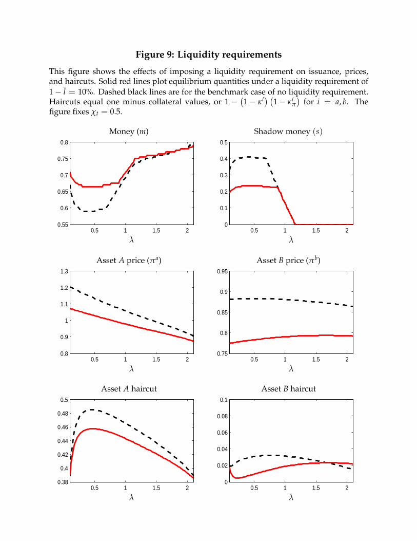
Figure 9: Liquidity requirements

This figure shows the effects of imposing a liquidity requirement on issuance, prices,and haircuts. Solid red lines plot equilibrium quantities under a liquidity requirement of1− l = 10%. Dashed black lines are for the benchmark case of no liquidity requirement.Haircuts equal one minus collateral values, or 1 −

(1− κi) (1− κi

π

)for i = a, b. The

figure fixes χt = 0.5.

Money (m) Shadow money (s)

0.5 1 1.5 20.55

0.6

0.65

0.7

0.75

0.8

λ

0.5 1 1.5 20

0.1

0.2

0.3

0.4

0.5

λ

Asset A price (πa) Asset B price (πb)

0.5 1 1.5 20.8

0.9

1

1.1

1.2

1.3

λ

0.5 1 1.5 20.75

0.8

0.85

0.9

0.95

λ

Asset A haircut Asset B haircut

0.5 1 1.5 20.38

0.4

0.42

0.44

0.46

0.48

0.5

λ

0.5 1 1.5 20

0.02

0.04

0.06

0.08

0.1

λ

Appendix

A Filtering

Let Ft represent agents’ information filtration. Agents form beliefs

λt = E[

λ̃t∣∣Ft

]. (A.1)

They learn about λ̃ from crash realizations and from uncertainty news. The solution tothe filtering problem with Markov switching is analyzed in Wonham (1965) and Liptserand Shiryaev (2001).

Uncertainty news are given by the process(λ̃− λ

)dt + σdB̃t. The crash realization

process is the uncompensated Poisson process dJ̃t, which must coincide with the observedcrash realization process dJt. The innovation to the household filtration Ft can thereforebe represented as the 2× 1 signal

dζt =

[ (λ̃t − λt

)dt + σdB̃t

dJ̃t − λtdt

], (A.2)

We seek to compute an innovations representation of the form

dλt = Atdt + B′tdζt. (A.3)

Note that

dλt = E[

λ̃t+dt∣∣Ft, dζt

]− E

[λ̃t∣∣Ft

](A.4)

= E[

λ̃t + dλ̃t∣∣Ft, dζt

]− E

[λ̃t∣∣Ft

](A.5)

=[−(

λt − λL)

qH +(

λH − λt

)qL]

dt + E[

λ̃t∣∣Ft, dζt

]− E

[λ̃t∣∣Ft

]. (A.6)

The last line follows from the fact that the crash and news innovations are uncorrelatedwith the switching process for λ̃. The innovation representation is therefore the condi-tional mean of the population regression

λ̃t − λt =[−(

λt − λL)

qH +(

λH − λt

)qL]

dt + B′tdζt + εt. (A.7)

The orthogonality condition for εt gives

Bt = E[

dζtdζ ′t∣∣Ft

]−1 E[

dζt(λ̃t − λt

)∣∣Ft]

(A.8)

=

[σ2dt 0

0 λtdt

]−1 [ (λH − λt

) (λt − λL) dt(

λH − λt) (

λt − λL) dt

](A.9)

=

[1

σ21λt

] (λH − λt

) (λt − λL

). (A.10)

Therefore, we can write the dynamics of the perceived crash intensity as

dλt =[−(

λt − λL)

qH +(

λH − λt

)qL]

dt +(

λH − λt

) (λt − λL

) [1

σ21λt

]dζt

(A.11)

=[−(

λt − λL)

qH +(

λH − λt

)qL]

dt +(

λH − λt

) (λt − λL

)(dBt

σ+

dNt

λt

),

(A.12)

where dBt =1σ

(λ̃t − λt

)dt + dB̃t is a Brownian motion and dNt = dJ̃t − λtdt = dJt − λtdt

is a compensated Poisson jump process with intensity λt, both adapted to Ft. Thus,

dλt

(λH − λt) (λt − λL)=

(− qH

λH − λt+

qL

λt − λL

)dt +

1σ

dBt +1λt

dNt. (A.13)

This confirms (3).

B Liquidity and information sensitivity

We show how to motivate our definition of liquidity as a sufficient condition for avoidinginformation acquisition by arbitrageurs and the resulting adverse selection problem.

Consider an arbitrageur who runs a fund with assets under management normalizedto one. For simplicity, assume that the fund is short-lived so its investment horizon haslength dt. At the end of this period, the arbitrageur is compensated for outperforming aleverage-adjusted benchmark composed of the underlying assets.

We consider arbitrageurs in the equity and shadow money markets separately. Thisis without loss of generality as in equilibrium we will show that at any given state onlyone of the two markets is liquid (typically shadow money), ruling out informed arbitragetrades that exploit equity and shadow money simultaneously.

An equity fund trades money and equity, yielding a rate of return drS,t = drm,t +wt (dre,t − drm,t), where wt is the portfolio weight in equity. On the other hand, her bench-mark return is drI,t = drm,t + wt (dre,t − drm,t), where wt = Et [wt| λt]. In order to obtainfinite demand, suppose the fund faces a quadratic position cost α

2 (wt − wt)2. This means

that an infinite position is prohibitively expensive. This could be due to some form of riskaversion or more broadly decreasing returns to scale at the trading strategy level.

Let ϑt be the LaGrange multiplier for the constraint wt = Et [wt| λt]. An informedarbitrageur thus maximizes

VArbt dt = max

wtEt[

drS,t − drI,t| λ̃]− α

2(wt − wt)

2 dt + ϑt (wt − Et [wt| λt]) dt (B.1)

= maxwt

Et[(wt − wt) (dre,t − drm,t)| λ̃

]− α

2(wt − wt)

2 dt (B.2)

+ϑt (wt − Et [wt| λt]) dt.

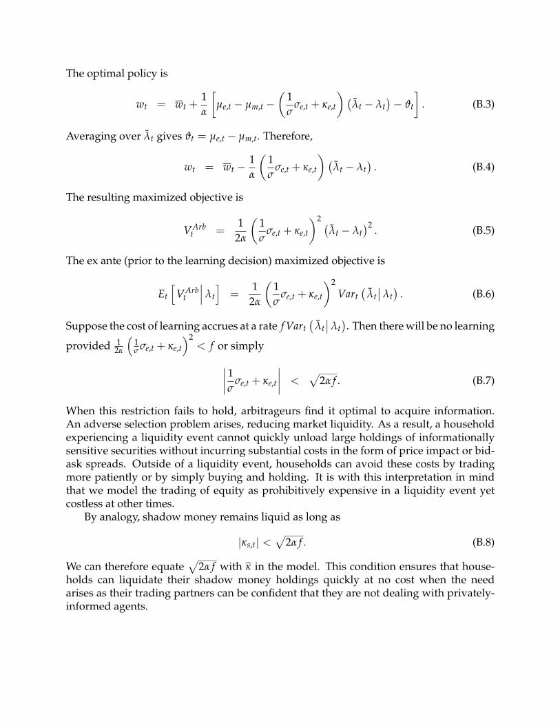
The optimal policy is

wt = wt +1α

[µe,t − µm,t −

(1σ

σe,t + κe,t

) (λ̃t − λt

)− ϑt

]. (B.3)

Averaging over λ̃t gives ϑt = µe,t − µm,t. Therefore,

wt = wt −1α

(1σ

σe,t + κe,t

) (λ̃t − λt

). (B.4)

The resulting maximized objective is

VArbt =

12α

(1σ

σe,t + κe,t

)2 (λ̃t − λt

)2 . (B.5)

The ex ante (prior to the learning decision) maximized objective is

Et

[VArb

t

∣∣∣ λt

]=

12α

(1σ

σe,t + κe,t

)2

Vart(

λ̃t∣∣ λt)

. (B.6)

Suppose the cost of learning accrues at a rate f Vart(

λ̃t∣∣ λt). Then there will be no learning

provided 12α

(1σ σe,t + κe,t

)2< f or simply∣∣∣∣ 1σ σe,t + κe,t

∣∣∣∣ <√

2α f . (B.7)

When this restriction fails to hold, arbitrageurs find it optimal to acquire information.An adverse selection problem arises, reducing market liquidity. As a result, a householdexperiencing a liquidity event cannot quickly unload large holdings of informationallysensitive securities without incurring substantial costs in the form of price impact or bid-ask spreads. Outside of a liquidity event, households can avoid these costs by tradingmore patiently or by simply buying and holding. It is with this interpretation in mindthat we model the trading of equity as prohibitively expensive in a liquidity event yetcostless at other times.

By analogy, shadow money remains liquid as long as

|κs,t| <√

2α f . (B.8)

We can therefore equate√

2α f with κ in the model. This condition ensures that house-holds can liquidate their shadow money holdings quickly at no cost when the needarises as their trading partners can be confident that they are not dealing with privately-informed agents.

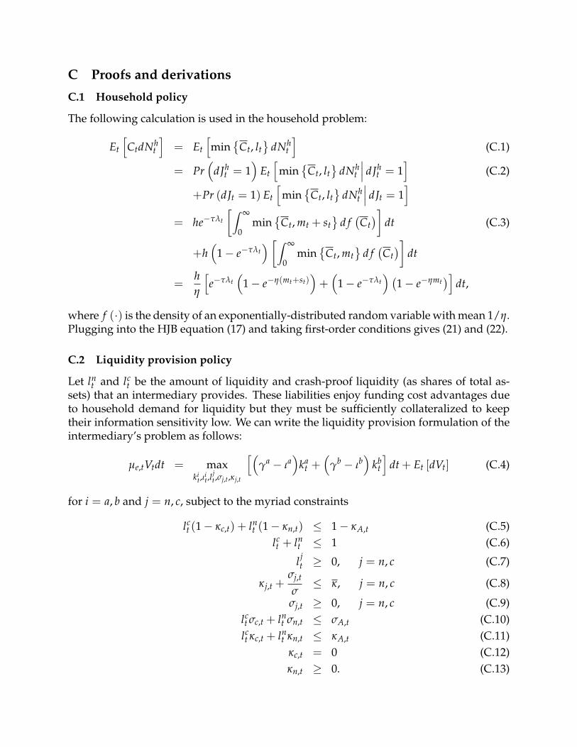
C Proofs and derivations

C.1 Household policy

The following calculation is used in the household problem:

Et

[CtdNh

t

]= Et

[min

{Ct, lt

}dNh

t

](C.1)

= Pr(

dJht = 1

)Et

[min

{Ct, lt

}dNh

t

∣∣∣ dJht = 1

](C.2)

+Pr (dJt = 1) Et

[min

{Ct, lt

}dNh

t

∣∣∣ dJt = 1]

= he−τλt

[∫ ∞

0min

{Ct, mt + st

}d f(Ct)]

dt (C.3)

+h(

1− e−τλt) [∫ ∞

0min

{Ct, mt

}d f(Ct)]

dt

=hη

[e−τλt

(1− e−η(mt+st)

)+(

1− e−τλt) (

1− e−ηmt)]

dt,

where f (·) is the density of an exponentially-distributed random variable with mean 1/η.Plugging into the HJB equation (17) and taking first-order conditions gives (21) and (22).

C.2 Liquidity provision policy

Let lnt and lc

t be the amount of liquidity and crash-proof liquidity (as shares of total as-sets) that an intermediary provides. These liabilities enjoy funding cost advantages dueto household demand for liquidity but they must be sufficiently collateralized to keeptheir information sensitivity low. We can write the liquidity provision formulation of theintermediary’s problem as follows:

µe,tVtdt = maxki

t,ιit,l

jt ,σj,t,κj,t

[(γa − ιa

)ka

t +(

γb − ιb)

kbt

]dt + Et [dVt] (C.4)

for i = a, b and j = n, c, subject to the myriad constraints

lct (1− κc,t) + ln

t (1− κn,t) ≤ 1− κA,t (C.5)lct + ln

t ≤ 1 (C.6)

l jt ≥ 0, j = n, c (C.7)

κj,t +σj,t

σ≤ κ, j = n, c (C.8)

σj,t ≥ 0, j = n, c (C.9)lct σc,t + ln

t σn,t ≤ σA,t (C.10)lct κc,t + ln

t κn,t ≤ κA,t (C.11)κc,t = 0 (C.12)κn,t ≥ 0. (C.13)

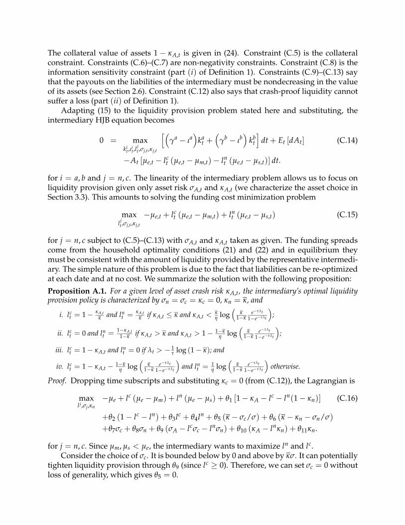
The collateral value of assets 1 − κA,t is given in (24). Constraint (C.5) is the collateralconstraint. Constraints (C.6)–(C.7) are non-negativity constraints. Constraint (C.8) is theinformation sensitivity constraint (part (i) of Definition 1). Constraints (C.9)–(C.13) saythat the payouts on the liabilities of the intermediary must be nondecreasing in the valueof its assets (see Section 2.6). Constraint (C.12) also says that crash-proof liquidity cannotsuffer a loss (part (ii) of Definition 1).

Adapting (15) to the liquidity provision problem stated here and substituting, theintermediary HJB equation becomes

0 = maxki

t,ιit,l

jt ,σj,t,κj,t

[(γa − ιa

)ka

t +(

γb − ιb)

kbt

]dt + Et [dAt] (C.14)

−At [µe,t − lct (µe,t − µm,t)− ln

t (µe,t − µs,t)] dt.

for i = a, b and j = n, c. The linearity of the intermediary problem allows us to focus onliquidity provision given only asset risk σA,t and κA,t (we characterize the asset choice inSection 3.3). This amounts to solving the funding cost minimization problem

maxl jt ,σj,t,κj,t

−µe,t + lct (µe,t − µm,t) + ln

t (µe,t − µs,t) (C.15)

for j = n, c subject to (C.5)–(C.13) with σA,t and κA,t taken as given. The funding spreadscome from the household optimality conditions (21) and (22) and in equilibrium theymust be consistent with the amount of liquidity provided by the representative intermedi-ary. The simple nature of this problem is due to the fact that liabilities can be re-optimizedat each date and at no cost. We summarize the solution with the following proposition:

Proposition A.1. For a given level of asset crash risk κA,t, the intermediary’s optimal liquidityprovision policy is characterized by σn = σc = κc = 0, κn = κ, and

i. lct = 1− κA,t

κ and lnt =

κA,tκ if κA,t ≤ κ and κA,t <

κη log

(κ

1−κe−τλt

1−e−τλt

);

ii. lct = 0 and ln

t =1−κA,t

1−κ if κA,t > κ and κA,t > 1− 1−κη log

(κ

1−κe−τλt

1−e−τλt

);

iii. lct = 1− κA,t and ln

t = 0 if λt > − 1τ log (1− κ); and

iv. lct = 1− κA,t − 1−κ

η log(

κ1−κ

e−τλt

1−e−τλt

)and ln

t = 1η log

(κ

1−κe−τλt

1−e−τλt

)otherwise.

Proof. Dropping time subscripts and substituting κc = 0 (from (C.12)), the Lagrangian is

maxl j,σj,κn

−µe + lc (µe − µm) + ln (µe − µs) + θ1 [1− κA − lc − ln(1− κn)] (C.16)

+θ2 (1− lc − ln) + θ3lc + θ4ln + θ5 (κ − σc/σ) + θ6 (κ − κn − σn/σ)

+θ7σc + θ8σn + θ9 (σA − lcσc − lnσn) + θ10 (κA − lnκn) + θ11κn.

for j = n, c. Since µm, µs < µe, the intermediary wants to maximize ln and lc.Consider the choice of σc. It is bounded below by 0 and above by κσ. It can potentially

tighten liquidity provision through θ9 (since lc ≥ 0). Therefore, we can set σc = 0 withoutloss of generality, which gives θ5 = 0.

Next, consider the choice of σn. It can only tighten liquidity provision through θ6 orθ9 so we can set σn = 0 without loss of generality. This implies θ9 = 0.

To determine κn, we will first show that θ1 always binds. Suppose θ1 is slack. Then θ2must bind since if it does not lc can be raised further (recall σc = 0). Thus if θ1 is slack,θ2 must bind. But then it is profitable to raise lc and reduce ln one-for-one since lc has agreater funding advantage (ln > 0 since otherwise lc = 1 and θ1 would be violated). Weconclude that θ1 binds.

Now back to κn: Note that since θ1 binds, 1− κA = lc + ln (1− κn), and since ln + lc ≤1, we automatically have lnκn ≤ κA so θ10 is always satisfied and therefore redundant.This means that it is unambiguously better to raise κn so as to increase liquidity produc-tion. As κn is bounded from above by κ, we conclude κn = κ (and θ11 = 0).

Turning to ln and lc, we can now substitute σc = σn = 0, κn = κ, θ5 = θ9 = θ11 = 0, aswell as impose complementary slackness on θ6, θ7 and θ8, none of which involve ln or lc.We can also remove the redundant θ10. The Lagrangian simplifies to

maxln,lc

−µe + lc (µe − µm) + ln (µe − µs) (C.17)

+θ1 [1− κA − lc − ln(1− κ)] + θ2 (1− lc − ln) + θ3lc + θ4ln.

The optimality conditions are

µe − µm = θ1 + θ2 − θ3 (C.18)µe − µs = (1− κ) θ1 + θ2 − θ4. (C.19)

We already know θ1 > 0. Since µe − µm > µe − µs, we also have κθ1 > θ3 − θ4.Case (i): Suppose θ2 > 0 so ln + lc = 1. Since θ1 > 0, ln = κA/κ and so lc =

1 − κA/κ. This clearly requires κA ≤ κ and gives θ3 = θ4 = 0. Substituting for thespreads from the household problem, θ1 = 1

κ h (ψ− 1)(1− e−τλ

)e−η(1−κA/κ) and θ2 =

h (ψ− 1)[e−τλe−η +

(1− 1

κ

) (1− e−τλ

)e−η(1−κA/κ)

]. For θ2 to be positive, this also re-

quires κA < κη log

(κ

1−κe−τλ

1−e−τλ

).

Case (ii): Suppose θ3 > 0 so lc = 0. Then θ2 = 0 by case (i). Since θ1 > 0,ln = (1− κA) / (1− κ). For θ2 = 0, we must have κA > κ. It follows that θ4 = 0.

Substituting for the spreads gives θ3 = h (ψ− 1)[

κ1−κ e−τλe−η

(1−κA1−κ

)−(1− e−τλ

)]and

θ1 = h (ψ− 1) 11−κ e−τλe−η

(1−κA1−κ

). Since θ3 > 0, κA > 1− 1−κ

η log(

κ1−κ

e−τλ

1−e−τλ

).

Case (iii): Suppose θ4 > 0 so ln = 0. Then θ2 = 0 by case (i). Since θ1 > 0, lc =

1− κA and so θ2 = θ3 = 0. Substituting for the spreads, θ1 = h (ψ− 1) e−η(1−κA) andθ4 = h (ψ− 1)

[(1− κ)− e−τλ

]e−η(1−κA). This case thus requires λ > − 1

τ log (1− κ) (sothat θ4 > 0).

Case (iv): Suppose θ2 = θ3 = θ4 = 0. Since θ1 > 0, ln = 1− κA + lnκ− lc. Substitutingfor the spreads and solving, ln = 1

η log(

κ1−κ

e−τλ

1−e−τλ

), lc = 1− κA − 1−κ

η log(

κ1−κ

e−τλ

1−e−τλ

),

and θ1 = h (ψ− 1) e−η(1−κA)(

e−τλ

1−κ

)1−κ (1−e−τλ

κ

)κ.

We can now show that the optimal liquidity provision policy characterized in Propo-sition A.1 can be implemented with crash-proof liquid money, liquid shadow money, andilliquid equity as stated in Proposition 1 in the text:

Proof of Proposition 1. We already showed that κs,t = κ is optimal for delivering normal-times liquidity.

Case (i): The optimal capital structure can be implemented with mt = 1− κA,tκ and

st =κA,t

κ . This case technically requires an infinite σe,t but in practice it can be imple-mented with an arbitrarily small amount of equity and finite σe,t with no impact on theequilibrium. Equity is illiquid.

Case (ii): The optimal capital structure can be implemented with mt = 0 and st =1−κA,t

1−κ . Equity is et =κA,t−κ

1−κ with κe,t = 1 so equity is illiquid.Case (iii): The optimal liquidity supply can be implemented with mt = 1− κA,t and

st = 0. Equity is 1− mt − st = κA,t and is wiped out in a crash (κe,t = 1) so equity isilliquid.

Case (iv): The optimal capital structure can be implemented with mt = (1− κA,t)−1−κ

η log(

κ1−κ

e−τλt

1−e−τλt

)and st =

1η log

(κ

1−κe−τλt

1−e−τλt

). Equity is again wiped out in a crash,

κe,t = 1 so it is illiquid.

C.3 Asset-side policy

From (14) and (15), applying Ito’s Lemma to total assets and dropping time subscripts,the asset-side intermediary problem is

0 = maxka,kb,ιa,ιb

(γa − ιa

)ka +

(γb − ιb

)kb + πaka

[µa

π + φ(

ιa)− δ + κaκa

πλ]

(C.20)

+πbkb[µb

π + φ(

ιb)− δ + κbκb

πλ]− A [µe − θ1 (1− κA)− θ2] ,

where θ1 is the multiplier on the collateral constraint and θ2 is the multiplier on the equitycapital requirement (both are scaled by assets). We have already substituted the liabilities-side optimality conditions (C.18) and (C.19). The multipliers θ1 and θ2 are determinedin equilibrium by aggregate liquidity provision and collateral values, their formulas areincluded in the proof of Proposition A.1.

Taking derivatives of (C.20) with respect to ιa and ιb gives (26). Substituting for κAusing (24) and differentiating with respect to ka and kb gives (25).

D Numerical solution

Using the adjustment cost function φ (ι) = 1ϕ

(√1 + 2ϕι− 1

), the optimality conditions

for capital (25) become

µe − θ1

(1− κi

π

) (1− κi

)− θ2 =

γi + 12ϕ

πi +πi

2ϕ+ µi

π −1ϕ− δ + κiκi

πλ (D.1)

for i = a, b. The multipliers are provided in the proof of Proposition A.1. Substitutingfor the investment cost function and the investment optimality conditions into (27), thedynamics of χ are

dχ = µ (1− 2χ) dt + χ (1− χ)

[πa − πb

ϕ+ λ

(κa − κb

)]dt (D.2)

−χ (1− χ)

[κa − κb

χ (1− κa) + (1− χ)(1− κb

)] dJ.

To get the dynamics of prices, apply Ito’s Lemma:

dπi

πi =

[πi

λ

πi

(λ− λL

) (λH − λ

)(− qH

λH − λ+

qL

λ− λL − 1)

(D.3)

+12

πiλλ

πi

(λ− λL

)2 (λH − λ

)2 1σ2 +

πiχ

πi χ (1− χ)

(µ

(1χ− 1

1− χ

)+

πa − πb

ϕ+ λ

(κa − κb

))]dt +

πiλ

πi

(λ− λL

) (λH − λ

) 1σ

dB

−

1−πi(

λ + 1λ

(λ− λL) (λH − λ

), χ− χ(1−χ)(κa−κb)

χ(1−κa)+(1−χ)(1−κb)

)πi

dJ

for i = a, b. We solve for πa and πb using Chebyshev collocation.

E Conditional state density

Let ft (λ, χ) be the joint density of λ and χ at t given initial density f0 (λ, χ). We calculatef by solving the associated forward Kolmogorov equation (Hanson, 2007, Theorem 7.7):

∂ ft

∂t= − ∂

∂λ(µλ ft)−

∂

∂χ(µχ ft) +

12

∂2

∂λ2

(σ2

λ ft

)(E.1)

+

[λ− ft

(λ−, χ−

) ∣∣∣∣∂λ−

∂λ

∣∣∣∣ ∣∣∣∣∂χ−

∂χ

∣∣∣∣− λ ft (λ, χ)

].

We have

∂

∂λ(µλ ft) =

[2λ−

(qH + qL

)−(

λH + λL)]

ft (E.2)

+[−qH

(λ− λL

)+ qL

(λH − λ

)−(

λ− λL) (

λH − λ)] ∂ ft

∂λ∂

∂χ(µχ ft) =

[1ϕ

(πa − πb

)+ λ

(κa − κb

)] [(1− 2χ) ft + χ (1− χ)

∂ ft

∂χ

](E.3)

+µ

[(1− 2χ)

∂ ft

∂χ− 2 ft

]+

1ϕ

(πa

χ − πbχ

)χ (1− χ) ft

∂2

∂λ2

(σ2

λ ft

)= 2

[(∂σλ

∂λ

)2

+ σλ

(∂2σλ

∂λ2

)]ft + 4σλ

(∂σλ

∂λ

)∂ ft

∂λ+ σ2

λ

∂2 ft

∂λ2 , (E.4)

where σλ =(λ− λL) (λH − λ

) 1σ , ∂σλ

∂λ =(λL + λH − 2λ

) 1σ , and ∂2σλ

∂λ2 = − 2σ . The pre-jump

state values λ− and χ− are given by

λ− =λLλH

λL + λH − λ(E.5)

χ− =1

1 +(

1−κa

1−κb

) (1−χ

χ

) (E.6)

with ∂λ−∂λ = λLλH

(λL+λH−λ)2 and ∂χ−

∂χ =

(1−κa

1−κb

)(1

χ2

)[1+(

1−κa

1−κb

)(1−χ

χ

)]2 . We solve the Kolmogorov equation

with Chebyshev collocation as in the rest of the paper.

F Implementation of policy interventions

F.1 Large Scale Asset Purchases

Let ζt ∈ {ζE, ζF} denote the state of the central bank’s balance sheet which is either“empty” (ζt = ζE) or “full” (ζt = ζF). An empty balance sheet is filled with probabil-ity βLSAP(λt, χt) immediately after a crash in which case it becomes full. The size of theprogram is given as a state-contingent fraction α(λt, χt) of the outstanding supply of Acapital. A full balance sheet is emptied (ζt = ζE) with intensity βTAPER(λt, χt).

We nest a permanent and transitory LSAP programs with βTAPER (λt, χt) = 0 undera permanent policy and βTAPER (λt, χt) > 0 under a transitory policy. We can expressprices as πi

t = πi (λt, χt, ζt) for i = a, b. The drift and after-crash value of prices whenζt = ζE are

µiπ,ζE

= µiπ,ζ0− λβLSAP

(κi

π,LSAP − κiπ

)(F.1)

1− κiπ,ζE

= min{

1− κiπ,LSAP, 1− κi

π

}, (F.2)

for i = a, b where µiπ,ζ0

is given in (D.3), 1 − κiπ,LSAP = πi(λ+,χ+−α,ζF)

π(λ,χ,ζE)(LSAP shifts χ+

to χ+ − α), and 1− κiπ = π(λ+,χ+,ζE)

π(λ,χ,ζE). These modified dynamics enter into (25). Under

ζt = ζF, we have

µiπ,ζF

= µiπ,ζ0− βTAPERκi

π,TAPER. (F.3)

for i = a, b with 1− κπ,TAPER = π(λ,χ+α,ζE)πi(λ,χ,ζF)

. To keep things simple, we do not imposecollateral constraints with respect to the reversal shock. This has the effect of understatingthe impact of policy withdrawal. In addition, the policy’s entry and exit are generally notof equal size as the economy drifts in the meantime. In this case one can think of thecentral bank’s balance sheet as retaining a residual position.

We measure the announcement effect of an LSAP program as the difference in crashreturns with and without the intervention, κi

π − κiπ,LSAP. A policy reversal shock is mea-

sured analogously as πi(λ,χ−α,ζE)πi(λ,χ,ζF)

− 1. We measure the effect of an unanticipated tapering

shock that raises βTAPER as πi(λ,χ,ζF|βHTAPER)

πi(λ,χ,ζF|βLTAPER)

− 1.

In the case of a permanent intervention, the economy at ζt = ζF corresponds to thebenchmark economy and we can solve backwards to obtain prices under ζE. When inter-ventions are transitory, there is two-way flow between ζE and ζF and we solve for pricesunder the two regimes simultaneously.

F.2 Operation Twist

We map the safe capital kbt to government debt by assuming that the private sector cannot

create it but that the government issues it at the same rate as in the baseline model.35 Tomodel a change in duration within a given economy, we split type kb capital into twopieces: zero-duration floating-rate debt k f b and long-duration safe bonds klb (so kb

t =

k f bt + klb

t ). Floating debt pays the floating rate µm (the yield of money) and trades at parin equilibrium. Long bonds pay the fixed coupon γb as in the baseline model. We avoidintroducing an additional state variable by assuming that the central bank sets the relativeshares αt = k f b

t /kbt and 1− αt = klb

t /kbt as a policy variable.

In an Operation Twist intervention, the central bank buys long-term bonds and sellsfloating rate bonds of equal dollar amounts at post-announcement prices. This changestheir relative shares αt and 1− αt. Operation Twist thus changes the composition of gov-ernment debt αt, while keeping its value constant. The change in the quantity of govern-ment debt is characterized as follows.

Let x− and x+ denote the pre- and post-intervention values of a given quantity x. Forexample πbl

+ is the post-intervention price of the long-term bond. Assuming that the gov-ernment trades at post-announcement prices and that the intervention does not change

35Specifically, private investment ιbt is restricted to zero in the pricing equation (25). Existing long bondsdepreciate on the balance sheet but the government controls their aggregate supply by setting issuance todklb

t =[φ(

ιlbt

)− δ]

dt absent a policy shock with πlbt φ′

(ιlbt

)= 1 and similarly for dk f b

t .

the overall value of government liabilities, the pre- and post- quantities must respect

kb−

[α−π

f b+ + (1− α−)πlb

+

]= kb

+

[α+π

f b+ + (1− α+)πlb

+

]. (F.4)

We solve for net new issuance kb+

kb−

as a function of equilibrium prices and the change in

the debt maturity mix α+ − α−.

F.3 Liquidity requirements

The solution to the intermediary capital structure problem in the presence of a liquidityrequirement is characterized by

Proposition F.1. Let l be the upper bound on liquidity creation. The intermediary’s optimalliquidity provision policy is implemented by

i. mt = l and st = 0 if κA,t ≤ 1− l;

ii. mt = l − κA,t−(1−l)κ and st =

κA,t−(1−l)κ if 1 − l ≤ κA,t ≤ 1 − l + κl and κA,t <

1− l + κη log

(κ

1−κe−τλt

1−e−τλt

);

iii. mt = 0 and st =1−κA,t

1−κ if κA,t > 1− l + κl and κA,t > 1− 1−κη log

(κ

1−κe−τλt

1−e−τλt

);

iv. mt = 1− κA,t and st = 0 if λt > − 1τ log (1− κ) and κA,t ≥ 1− l;

v. mt = (1− κA,t)− 1−κη log

(κ

1−κe−τλt

1−e−τλt

)and st =

1η log

(κ

1−κe−τλt

1−e−τλt

)otherwise.

Proof of Proposition F.1. The proof follows the recipe for Propositions A.1 and 1, replacingthe limited liability constraint with the liquidity requirement. The only new case is case(i) which arises when total risk is so low that the solution in case (ii) would violate theliquidity requirement.