coastal research and policy integration corepoint – eu ...corepoint.ucc.ie/2.3 quantification of...

QUANTIFICATION OF THE ECONOMIC BENEFITS OF NATURAL COASTAL ECOSYSTEMS

Coastal Research and Policy Integration

COREPOINT – EU-INTERREG IIIB

Activity 2.3

Revised January 2007

Activity 2.3: Quantify the economic benefits of natural coastal ecosystems

of 37

EXECUTIVE SUMMARY

The European coastline includes a great diversity of geomorphologic features, ecosystem /

biome types, socio-economic dynamics and culture. This report provides an economic

valuation of the coastal and marine resources of the Member States from NW Europe involved

in the COREPOINT-INTERREG IIIB project. Using an ecosystem service value method for

valuation, the analysis estimates the economic value in 2003 of the coastal and marine zone of

Belgium as €256M, Ireland €11,700M, France €18,405M, Netherlands €4,005M and the UK as

€65,325M. This equates to the following percentage of GNI (Global National Income); Ireland

9.6%, UK 3.4%, France 1.1%, Netherlands 0.8% and Belgium < 0.1%,

Whilst these valuations are useful for high-level strategic and policy considerations, they do not

provide much insight for ICZM practitioners. Consequently, a method based on normative

economics rather than ecological economics was designed; this method was called Biodiversity

Portfolio Analysis. This method assesses the risk to the provision of ecosystem services and

the economic return of those services, using the portfolio of different biomes types within the

target Members State’s coastal and marine zone. The analysis is based upon the

interrelationships of risk and return between different biomes, weighted by area; it provides a

comparative risk and return index for each Member State.

The Biodiversity Portfolio Analysis for the target Members States showed that risk and return

were highly correlated in the studied Members States. The ranking of risk and return, with the

highest first, was Ireland > UK > France = Netherlands > Belgium. For these Member States

the risks to ecosystem service provision were positively correlated with GNI (r = 0.97, P<0.01);

suggesting that the higher the economic importance of coastal and marine resources in a

Member State the more at risk the resources are.

A smaller spatial scale case study is also presented from Durham Heritage Coast which

illustrates the use of this technique in prioritisation of management actions at a local scale.

Using stakeholder involvement to determine risks and returns, the case study identifies key

biomes and key risks to those biomes which would negatively impact upon ecosystem service

provision from the case study area.

Although, the Biodiversity Portfolio Technique involves making a number of assumptions, it

does provide coastal managers with a potential tool with which to strategically plan due to

increased awareness of the interaction between the elements of the portfolio of biomes. It is

proposed that this technique could be easily adapted for use at local or regional spatial scales

in areas where ICZM initiatives are being implemented.


of 37

TABLE OF CONTENTS

CHAPTER 1: ECONOMIC VALUATION OF NW EUROPEAN COAST 6

1.1 Introduction

1.2 Economic valuation of biodiversity in NW Europe

1.3 Annual Values of Ecosystem Service

6

6

7

CHAPTER 2: BIODIVERSITY PORTFOLIO APPROACH 9

2.1 Introduction to portfolio method

2.2 Hypothetical Biodiversity Portfolio analysis

2.3 Risk to ecosystem service provision

2.4 Interpretation of Risk-Return Profiles

2.5 Trading off risks to maintain returns.

2.6 Correlation between risk factors

9

9

11

13

14

14

CHAPTER 3: BIODIVERSITY PORTFOLIO ANALYSIS OF NW EUROPE 17

3.1 Portfolio analysis 17

CHAPTER 4: MEMBER STATE SCALE APPLICATION OF THE BIODIVERSITY PORTFOLIO

APPROACH 21

4.1 Assumptions of the Portfolio method.

4.2 Benefits of the Portfolio Method for ICZM.

4.3 Application of the Portfolio Method for ICZM.

21

22

22

CHAPTER 5: A LOCAL-SCALE CASE STUDY USING THE BIODIVERSITY PORTFOLIO

APPROACH 24

5.1 Durham Heritage Coast study area. 5.2 Methodology 5.3 Results 5.4 Discussion and interpretation 5.5 Conclusions

24

25

26

33

36

ACKNOWLEDGMENTS 37


of 37

FIGURES AND TABLES

List of Figures

Figure 1. Risk-Return profile for each hypothetical Member State for each biome and cumulative (Total) for (a) Member State 1 and (b) Member State 2.

13

Figure 2. Revised Risk return graph for MS1 (Open Ocean O1 for original , O2 with over fishing no more a threat; Total portfolio T1 original; T2 with no over fishing threat).

16

Figure 3. Risk return relationship for COREPOINT Member States. Continental shelf biomes removed. Axes are nominal values but comparative.

18

Figure 4. Positive relationship between risk and GNI for target Member States (r = 0.97, P<0.01) (Key: Be, Belgium; Ne, Netherlands; Fr, France; UK, United kingdom and Ir, Ireland).

19

Figure 5. The location of the Durham Heritage Coast.

24

Figure 6. Risk-return profile for the Durham Heritage coast.

28

Figure 7. Re-worked risk-return profiles showing the impact of hypothetical management strategies aimed to target and reduce the risk of tourism and recreation impact.

30

Figure 8. Re-worked risk-return profile showing the impact of hypothetical management strategies aimed to reduce the risk of tourism and recreation impact and coastal erosion and sediment movement processes.

31

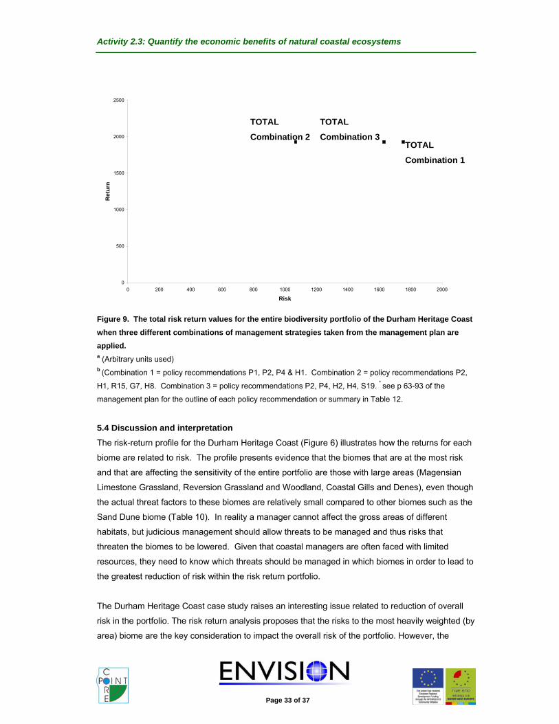
Figure 9. The total risk return values for the entire biodiversity portfolio of the Durham Heritage Coast when three different combinations of management strategies taken from the management plan are applied.

33


of 37

List of Tables

Table 1. Coastline and shelf zones of NW European countries 6

Table 2. Value of biomes by considering 17 ecosystem services of NW Europe member states from 1988 data and adjusted to 2003 values using Member State inflation rates.

7

Table 3. Value of coastal ecosystems per capita. 8

Table 4. Biodiversity portfolio of 2 hypothetical Member States 10

Table 5 Estimated ecosystem service function for the biomes present in the two hypothetical Member States.

10

Table 6. Categories of Systemic and Non-systemic threats. 11

Table 7. Correlation between risk factors for each biome. 14

Table 8. Percentage of three coastal biomes in target Member States (data from EU Demonstration Project)

17

Table 9. Estimated ecosystem service function for the biomes present on the Durham Heritage Coast.

26

Table 10. Categories of Systemic and Non-systemic threats 27

Table 11. Pearson’s correlation of the threat factors for each of the biomes leads to the resultant matrix of r2 values

28

Table 12. The ‘Independent’ pairs of biomes in the biodiversity portfolio. 29

Table 13. The ‘Associated’ pairs of biomes in the biodiversity portfolio 29

Table 12. The actions involved in the three coastal management scenarios.

32


of 37

CHAPTER 1: ECONOMIC VALUATION OF NW EUROPEAN COAST

1.1 Introduction Although there are a number of methodologies for quantitative assessment of the value of the

environment, these tend to give different results and there is a fundamental problem in assessing

non-use values, in particular “existence” value. Coupled to methodological issues, there is also a

scarcity of large scale data that can be used for such a valuation, for example, not all Member

States of Europe have a detailed biodiversity/biotope map of their territorial waters. An additional

problem is that, because so many “guesstimates” have to be used, then the “real” economic value

in absolute terms is very questionable – and most ecological economists spend the majority of their

time arguing over this. However, in order to decide management options that inevitably include an

element of compromise between competing interests and goals, absolute values of environmental

assets may be limited. A methodology that determines the relative value between management

scenarios based on the portfolio of different elements of the environment present within a Member

State’s boundaries and the dependence/interdependence between them is likely to be more

insightful. In this report we summarise firstly the outcomes from a study to determine the value of

Europe’s coasts as part of the EU ICZM Demonstration Project and, secondly, a proposed

methodology that uses a biodiversity portfolio approach.

1.2 Economic valuation of biodiversity in NW Europe

There are over 350,000 km of coastline within the 13 “old”-EU Member States with direct access to

the sea (Table 1); with a great diversity of coastline lengths, biome types and socio-economic

structures. There is considerable variety in coastline length among the Member States of the

COREPOINT partners, ranging from only 76Km for Belgium to over 19,000Km for the UK.

Table 1. Coastline and shelf zones of NW European countries (from: World Resources Institute; http://earthtrends.wri.org/; accessed May 2005). Length of Coastline was derived from the World Vector Shoreline database of the United States Mapping Agency; estimates calculated using a Geographic Information System (GIS) with a resolution of 1:250,000 kilometers and an underlying database consistent for the entire world.

Member State Length coastline (Km)

Belgium 76

Ireland 6,437

France 7,330

Netherlands 1,914

UK 19,717

“OLD” EUROPE 353,892

WORLD 1,634,701


of 37

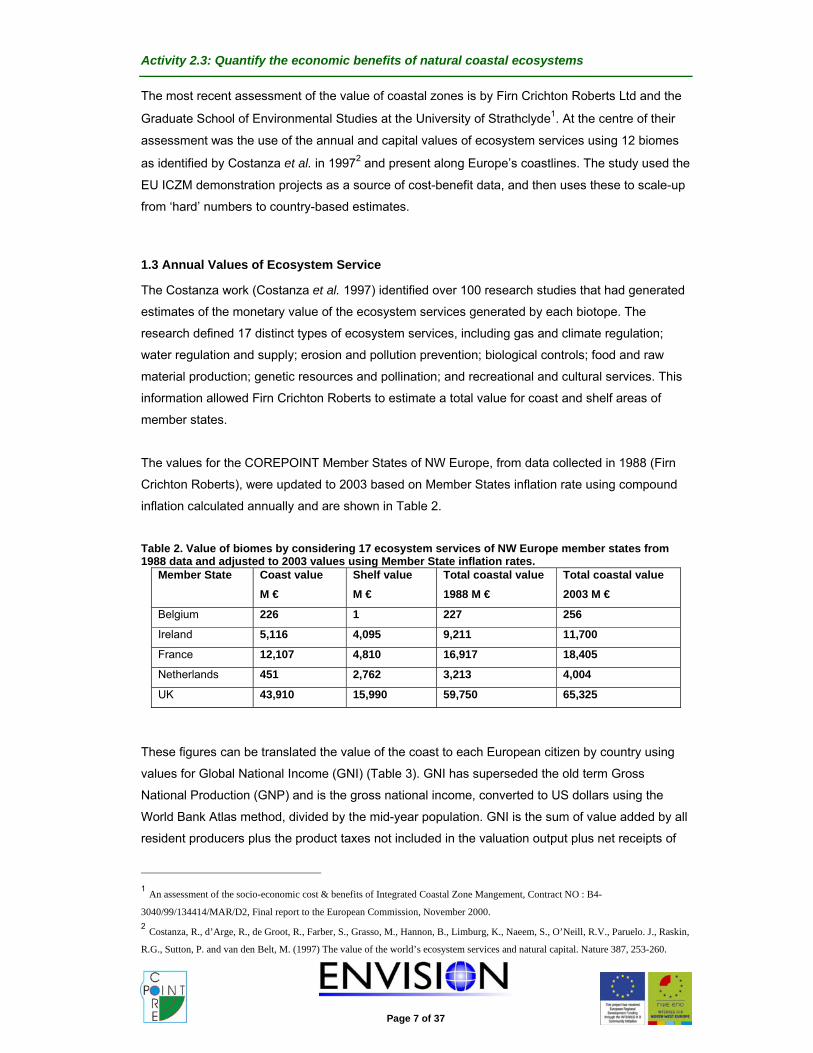
The most recent assessment of the value of coastal zones is by Firn Crichton Roberts Ltd and the

Graduate School of Environmental Studies at the University of Strathclyde1. At the centre of their

assessment was the use of the annual and capital values of ecosystem services using 12 biomes

as identified by Costanza et al. in 19972 and present along Europe’s coastlines. The study used the

EU ICZM demonstration projects as a source of cost-benefit data, and then uses these to scale-up

from ‘hard’ numbers to country-based estimates.

1.3 Annual Values of Ecosystem Service

The Costanza work (Costanza et al. 1997) identified over 100 research studies that had generated

estimates of the monetary value of the ecosystem services generated by each biotope. The

research defined 17 distinct types of ecosystem services, including gas and climate regulation;

water regulation and supply; erosion and pollution prevention; biological controls; food and raw

material production; genetic resources and pollination; and recreational and cultural services. This

information allowed Firn Crichton Roberts to estimate a total value for coast and shelf areas of

member states.

The values for the COREPOINT Member States of NW Europe, from data collected in 1988 (Firn

Crichton Roberts), were updated to 2003 based on Member States inflation rate using compound

inflation calculated annually and are shown in Table 2.

Table 2. Value of biomes by considering 17 ecosystem services of NW Europe member states from 1988 data and adjusted to 2003 values using Member State inflation rates.

Member State Coast value M €

Shelf value M €

Total coastal value 1988 M €

Total coastal value 2003 M €

Belgium 226 1 227 256

Ireland 5,116 4,095 9,211 11,700

France 12,107 4,810 16,917 18,405

Netherlands 451 2,762 3,213 4,004

UK 43,910 15,990 59,750 65,325

These figures can be translated the value of the coast to each European citizen by country using

values for Global National Income (GNI) (Table 3). GNI has superseded the old term Gross

National Production (GNP) and is the gross national income, converted to US dollars using the

World Bank Atlas method, divided by the mid-year population. GNI is the sum of value added by all

resident producers plus the product taxes not included in the valuation output plus net receipts of

1 An assessment of the socio-economic cost & benefits of Integrated Coastal Zone Mangement, Contract NO : B4-

3040/99/134414/MAR/D2, Final report to the European Commission, November 2000. 2 Costanza, R., d’Arge, R., de Groot, R., Farber, S., Grasso, M., Hannon, B., Limburg, K., Naeem, S., O’Neill, R.V., Paruelo. J., Raskin,

R.G., Sutton, P. and van den Belt, M. (1997) The value of the world’s ecosystem services and natural capital. Nature 387, 253-260.


of 37

primary income from abroad. The difference between GNI and GNP is that GNI includes member

State nationals who produce both for their nation’s economy as well as foreign interests in other

countries. The World Bank Atlas method for GNI averages inter-annual exchange rates for the

target year, by the preceding two years, adjusted by inflation rates. Table 3. Value of coastal ecosystems per capita.

Member State Global National

Income (GNI, €)*

Total value of

coastal

ecosystem

services (€ M)

% of GNI from

coastal

ecosystem

services

Annual value (€)

of coastal

ecosystems per

capita

Belgium 29,177 256 0.08 23

Ireland 30,465 11,700 9.60 2925

France 27,990 18,405 1.11 311

Netherlands 29,730 4,004 0.84 250

UK 32,036 65,325 3.46 1108

* figures are for 2003 from the World Development Indicators published by the World Bank. They have been converted from US Dollars to Euros, by using the mean monthly average exchange rate during 2003 (US$1 = €0.885).


of 37

CHAPTER 2: BIODIVERSITY PORTFOLIO APPROACH

2.1 Introduction to portfolio method

Valuing the ecosystem service value for Member States is useful to make comparisons between

the economic importance of the coastal and marine zone between Member States. However, it

does not provide ready information on which to base management strategies or operations. As an

alternative to estimating a total economic value for coastlines, we outline a methodology that

provides insight into the economic affect of loss of coastal biodiversity, and provides managers with

a tool that can be used for the basis of decision making within ICZM; this approach is based on

normative economics rather than ecological economics.

It is possible, that Cost-Benefit Analysis (CBA) could be used at a local scale, but the overriding

weighting of the very difficult to value “existence” costs for natural/protected area remains highly

problematic. The innovative technique outlined in the following chapters, has never previously

employed in coastal areas, is called portfolio modelling. The mathematics of portfolio analysis are

well known and used widely in equity fund management, in which a portfolio is developed that has

the highest return with the lowest risk.

The development of a biodiversity portfolio can be determined at the regional or national scale.

Risks for biotopes can be identified through known suites of threats and returns based on

previously published data adapted for use in the method. The key dynamics of the portfolio are

then based on the type of interaction between the biotope components which can be positively or

negatively correlated or display no significant association. Management of a biodiversity portfolio

can then be based upon decision making to maximize return for the minimum of risk. The sort of

management implications are that ICZM resources should be targeted to certain biotopes and it is

possible that these resources are not the most valuable but those that negate the most risk. Thus,

this analysis should provide an approach that doesn’t necessarily weight biotopes that are valuable

irrespective of the risk, but considers biotopes at a landscape scale and seeks to provide highest

return at minimum risk.

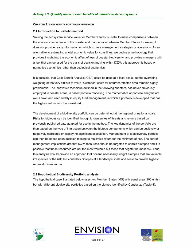
2.2 Hypothetical Biodiversity Portfolio analysis The hypothetical case illustrated below uses two Member States (MS) with equal area (100 units)

but with different biodiversity portfolios based on the biomes identified by Constanza (Table 4).


of 37

Table 4. Biodiversity portfolio of 2 hypothetical Member States (biome categories as used by Costanza et al. 1997)

Biome Member State 1 - Area

Member State 2 - Area

Open ocean 50 10

Continental Shelf 5 30

Tidal marshes 0 10

Floodplains 0 30

Temperate forest 30 0

Estuaries 15 20

TOTAL area 100 100

Each of the biomes provides a range of ecosystem services that are of value. Constanza broke

these service values down into 17 “types” and valued each in terms the presence of service and

extent of service. The service values varied between the biomes (Table 5). The table represents

estimated values for biome function, as no more quantified data is available. The figures are

agreed through the “expert opinion” of COREPOINT partners.

Table 5 Estimated ecosystem service function for the biomes present in the two hypothetical Member States. Scale from 0 = no or negligible ecosystem service provided; to 3 = extensive to complete service provided. Therefore, the maximum ecosystem “return” by any biome is 17 (no. of services) x 3 = 51. BIOME

SERVICE Open Ocean Shelf Marsh Floodplain Forest Estuary

Gas regulation 3 2 2 1 1 2

Climate regulation 3 2 1 1 1 2

Disturbance

regulation

2 2 2 2 0 3

Water regulation 1 1 2 3 2 3

Water supply 0 2 1 3 1 3

Erosion control &

sediment retention

2 3 3 2 1 3

Soil formation 1 2 2 3 2 2

Nutrient cycling 3 3 3 2 1 3

Waste treatment 2 3 2 2 0 3

Pollution 2 3 3 3 1 3

Biological control 0 0 0 0 1 0

Refugia 2 2 2 2 1 2

Food production 1 3 1 3 0 2

Raw materials 2 2 1 1 2 0

Genetic resources 2 2 1 1 1 2

Recreation 1 3 2 3 3 3

Cultural 0 1 1 3 2 1

TOTAL (out of 51) 27 36 29 35 20 37


of 37

2.3 Risk to ecosystem service provision

Any changes to the environment within any given biome – whether natural or anthropogenic in

origin – will produce a risk to the continuation of that service provision by the biome. Risk is defined

as the sum of the threats – the higher the cumulative threat score, the greater the severity of

threats, and consequent impact, the biome is likely to experience over time. Threat factors can be

divided into a number of categories (Table 6) depending on whether they are (i) Systemic threat

factors – larger than landscape scale risks that cannot be modified by management only mitigated

against (taken from EU demonstration project), and (ii) Non-systemic threat factors – risk factors

that are within landscape scale and risk factor can be modified in magnitude, or the impacts

mitigated against. The scale of any impact resulting from a threat factor can be tracked onto each

biome type present in the hypothetical Member State (Table 6). The value for each threat

component for each biome is agreed through the “expert opinion” of the COREPOINT partners.

Table 6. Categories of Systemic and Non-systemic threats. 0 = threat factor has no impact; to 5 = threat could destroy biome function. The maximum cumulative impact resulting from the combined threat factors is 18 (no of threat factors) x 5 = 80.

Open Ocean

Shelf Marsh Floodplain Forest Estuary

SYSTEMIC THREATS

Climate change 1 1 3 4 2 2

Sea level rise 0 0 5 4 1 4

NON-SYSTEMIC THREAT

Erosion 0 0 3 3 1 4

Sediment movement 0 0 4 3 1 5

Water pollution 0 1 2 3 0 4

Air pollution 0 0 1 1 1 1

Water shortage 0 0 0 3 1 3

Population growth 0 0 2 3 0 4

Tourism & recreation impact

0 3 2 4 1 4

Mineral extraction 2 3 1 1 0 2

Over-fishing 4 4 1 0 0 2

Transport congestion 0 3 0 0 0 5

Endangered species loss

2 2 1 1 1 3

Endangered migrants loss

0 1 4 3 1 4

Habitat loss 1 2 4 4 1 3

Urban expansion 0 3 2 5 2 4

TOTAL (out of possible 80)

10 23 35 42 13 54


of 37

Risk is the sum of the potential threat factors –Table 6 shows that an Open Ocean biome has less

cumulative threat factors and thus lower risk (10 nominal risk units) compared to an Estuary biome

(54).

The consequence of the risk faced by each hypothetical Member State to the provision of

ecosystem services is dependent upon the area of the biome present and the return (i.e., “value” of

the ecosystem services provided) provided by that biome. The RISK – RETURN profile of each

Member State will therefore be determined by the biome risk and return weighted by area:

(Eq 1) Biome Z risk for Member State = ∑Biome Z risk x biome Z area in Member State

(Eq 2) Biome Z return for Member State = ∑Biome Z return (i.e. ecosystem service value) x

biome Z area in Member State

The Biome portfolio risk and return are the cumulative weighted risk and returns for all the biomes

of the Member State; the values for risk and return are nominal values and are comparative. A

higher nominal risk value means that the biodiversity portfolio has a comparatively high associated

risk. Similarly, a higher nominal return value means that the biodiversity portfolio has a relatively

high comparative return.

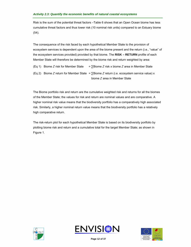
The risk-return plot for each hypothetical Member State is based on its biodiversity portfolio by

plotting biome risk and return and a cumulative total for the target Member State; as shown in

Figure 1.


of 37

2.4 Interpretation of Risk-Return Profiles Although the total return (ecosystem service value) for the biodiversity portfolio of both hypothetical

Member State’s is nearly the same (reference TOTAL in Fig.1 against Y axis), the risk is higher in

Member State 2 compared to Member State 1 (reference TOTAL in Fig.1 against X axis). This is

due to relatively large areas of floodplain and estuary that are relatively higher risk biomes. In

contrast, in Member State 1 the large area of Open Ocean provides a relatively high level of return

for minimal risk.

For a coastal manager, the biodiversity portfolio of Member State 1 is more attractive than that of

Member State 2 because for the same return on ecosystem service provision, the associated risk

from systemic and non-systemic threats is lower. However, in reality a coastal manager cannot

a

b

Figure 1. Risk-Return profile for each hypothetical Member State for each biome and cumulative (Total) for (a) Member State 1 and (b) Member State 2. The axes are nominal.


of 37

affect the gross areas of different habitats (i.e. make estuaries in open ocean), but judicious

management should allow threats to be managed and thus risks to be lowered. In a “real world” the

limited availability of resources, means that management should be targeted at biomes which lead

to the greatest reduction of risk. Further analysis of the biodiversity portfolio is thus required to

identity which threat(s) should be targeted in which biomes in order to minimise risk and maximise

return of the portfolio.

2.5 Trading off risks to maintain returns. The key to the biodiversity portfolio is the way in which risk can be traded off, i.e. risk on one biome

can balance risk on another. If a manager had only one biome then management would be clearly

targeted at reducing the key threat or threats to the biome. However, if a manager had 2 biomes –

would the risk profile be any better? This would depends on the way the two biomes relate to the

threat – if they both respond to threats in the same way then the risk profile is the same as with one

biome. However, assume another scenario in which one biome is resistant to a threat and one is

impacted heavily by a threat – then the two biome portfolio has less risk than a single biome as it

will still be producing a return even if the one of the biomes has been impacted by the threat. Thus

using this logic, the overall risk of a portfolio of two biomes that respond differently to threats is

lower compared to a portfolio with two biomes that respond in the same way; associated with this

lower risk is also the maintenance of return from the biodiversity portfolio.

2.6 Correlation between risk factors To determine which biomes respond in a similar way to threats, pairwise comparisons of biome

responses to threats were calculated. Pairwise correlation of the risk factors for each of the biome

pairs leads to the resultant matrix (Table 7) which provides information of the interaction between

biomes by risk.

Table 7. Correlation between risk factors for each biome. (*) = significant; (NS) = non-significant.

open shelf marsh flood forests

shelf 0.601 (*)

marsh -0.264 (NS) -0.383 (NS)

flood -0.536 (*) -0.317 (*) 0.631 (**)

forests -0.277 (NS) -0.194 (NS) 0.374 (NS) 0.651 (**)

estuaries -0.544 (*) -0.108 (NS) 0.302 (NS) 0.310 (NS) -0.078 (NS)

Where the correlation between any pair of biomes is not significant, then the threat factors for these

biomes are not related, i.e. they respond in an independent fashion to threat factors. These non

associated pairs are termed INDEPENDENT pairs.

Where the correlation between risk factors for a pair of biomes is significant and positive, then the

threat factors impact upon the biomes in a relatively similar way to the biomes, i.e. each of the two


of 37

biomes respond to threats in a similar way. These positive significant biome associations are

termed ASSOCIATED pairs.

Where the correlation between any pair of biomes is significant and negative, then threats that can

greatly impact upon ecosystem services in one biome tend to have little impact upon the other

biome. These are termed RESILIENT Pairs.

If an area had a portfolio made up of all INDEPENDENT pairs, then it would be possible to

passively manage risk, as even if returns from one biome are affected by a threat then they are not

associated to returns from others. In contrast, if a biome has a portfolio that consists only of

ASSOCIATED pairs then threats will impact all of the biome service provision producing an

inherently high risk portfolio. Alternatively, if a biome has a portfolio of RESILIENT biomes pairs

then risk to one biome can be offset against maintained service provision from the remainder. In

reality a real portfolio is likely to be a mix of different types of pairwise interactions that lead to

portfolio-wide reduction of risk.

For the hypothetical Member States illustrated here, the largest biome of Member State 1 is Open

Ocean (50 area units), which is ASSOCIATED to Shelf biomes (from Table 7.). The Estuary is

RESILIENT to threats in the Open Ocean and the forest is INDEPENDENT. This means that

realization of a threat in the Ocean will also impact be likely to impact the Coastal Shelf, but not

likely to impact Estuary. The Forest may or may not be impacted, depending on the nature of the

specific threat. Thus, the return from the portfolio is relatively robust to threats as the interactions

between the biomes and risk factors are offset by resilient pairs.

It is possible to indicate portfolio impact sensitivity by the sum of RESILIENT (which minimize risks

to returns) and INDEPENDENT (which are neutral) and pairs to ASSOCIATED pairs (which raise

risk in combination). Portfolio impact sensitivity can be calculated by the sum of the pairings with

scoring of: ASSOCIATED pairs= +1; RESILIENT pairs = -1; INDEPENDENT = 0. Thus for Member

State 1 this is:

ASSOCIATED pairs = +1 (Ocean & shelf)

RESILIENT pairs = -1 (Ocean & estuary)

INDEPENDENT pairs = 0 (Ocean & forest; shelf & forest; shelf & estuary; estuary & forest)

Giving a Portfolio impact sensitivity = 0

If we assume a scenario in which the management aim for Member State 1 would be to maximize

return and minimize the risk. Then taking the open Ocean, that has the highest biome return (low

return but large area), and knowing that changes in the Ocean are positively linked to Shelf and

that Estuaries are resilient to change in the open Ocean and that Forest act independently, then a

ban on over-fishing would reduce the threat portfolio of the Open Ocean by 4, making the risk to

ecosystem service change from 10 to 6. Reworking the weighted risk-return from the Member State


of 37

shows the impact of this management strategy on the risk-return profile (Figure 2).

The interpretation of this strategy is that through managing the threat of over-fishing the manager

has reduced the risk to services provided by the Open Ocean, but also reduced the risk to the

overall risk –return to all the biodiversity portfolio (T1 to T2).

For Member State 2, the risks are higher relative to Member State 1. Looking at the interaction in

the biome profile we find that the:

ASSOCIATED pairs = +2 (Ocean & shelf; marsh & flood)

RESILIENT pairs = -3 (Ocean & flood; ocean estuary; shelf & flood)

INDEPENDENT pairs = 0 (Ocean & marsh; shelf & marsh; shelf estuary; flood & estuary)

Giving a Portfolio impact sensitivity = -1

This means that there is a relatively higher level of biome pair association, i.e. the portfolio does

not lower risk because it has a relatively higher number of positive associated pairs that will

respond in a similar fashion in response to threats. Therefore a manager is faced with a portfolio

lacking robustness due to the association between biome pairs (or SECTORS). The priority for the

manager is to minimise risks to both of the associated pairs (Ocean & Shelf; Marsh & Flood).

Considering the threats table, one possibility is to choose a high impact threat that operates across

both sectors (relatively easy as they have ASSOCIATED impacts). For example, using the similar

calculations as above, assuming that the management strategy is to strictly control any tourism and

recreation impact, this would drop the inherent portfolio risk (Total) from 6.84 to 6.20.

Figure 2.Revised Risk return graph for MS1 (open Ocean O1 for original, O2 with over fishing no more a threat; Total portfolio T1 original; T2 with no over fishing threat). The Shelf Biome will also have lower risk, but the difference is too small to be displayed on this graph.


of 37

CHAPTER 3: BIODIVERSITY PORTFOLIO ANALYSIS OF NW EUROPE

3.1 Portfolio analysis

The previous Chapter has outlined the Biodiversity Portfolio method for two hypothetical Member

States. This Chapter outlines a comparative analysis of the target Member States (COREPOINT

partners) of NW Europe. Quantitative data availability for such an analysis remains a problem. This

is due to: firstly, a lack of biotope classification systems that links directly into the Costanza

Biotopes; and secondly to a lack of complete coverage of biotopes of the Members States,

especially the marine zone.

However, data is available with adequate coverage for these Members States from the EU

Demonstration Project from the work of Firn Crichton Roberts3. These data were “broad estimates”

of the percentage of the Constanza biomes in the coastal areas. Consequently, these data

represent an expert opinion, and remain to be validated by Europe-wide mapping in the future. As

this represents the most cohesive dataset covering all of the target Members States, it is used for

the following analysis. Raw data on the area of Costanza biomes from the EU Demonstration

Project was kindly provided by Dr John Firm of Firn Crichton Roberts. From these data, the biomes

with significant coastal inputs were selected: open ocean, continental shelf, tidal marsh, forest and

estuaries. The coastal areas include other biomes such as agriculture, but as they are nominally

influenced by coastal dynamics they were not considered. In addition, the area of open ocean was

zero for all Members States as all of the European marine zone was within the continental shelf.

Areas of biomes were changed into proportions of total coastal area and risk–return estimates were

calculated following precisely the method used in the previous chapter. However, due to the

comparatively large area of the continental shelf biome (95% or more for all target Member States),

the shelf biome had an overbearing influence on the risk and return estimates. Consequently, the

continental shelf biome was removed from the analysis and thus the analysis concentrated on the

remaining three coastal influenced biomes: tidal marsh, forest and estuaries. Risk return estimates

were calculated for the target Member States using the three coastal biomes. The data is shown in

Table 8 and the risk-return graph is shown in Fig. 3.

Table 8. Percentage of three coastal biomes in target Member States (data from EU Demonstration Project)

% of coastal biome Member State

Estuary Marsh Forest

France 4 17 79

Ireland 3 85 12

Netherlands 4 16 80

Belgium 6 0 94

UK 18 21 61

3 An assessment of the socio-economic cost & benefits of Integrated Coastal Zone Mangement, Contract NO : B4-

3040/99/134414/MAR/D2, Final report to the European Commission, November 2000.


of 37

15 20 25 30

21

22

23

24

25

26

27

28

Risk

Ret

urn

Fr

Ir

Ne

Be

UK

Figure 3. Risk return relationship for COREPOINT Member States. Continental shelf biomes removed. Axes are nominal values but comparative. (Key: Be, Belgium; Ne, Netherlands; Fr, France; UK, United kingdom and Ir, Ireland).

This analysis shows comparative differences in the risk-return status of the target Member States.

The graph shows a number of features:

• There is a high correlation between risk and return shown by the high correlation in risk

and return for the target Member States (r = 0.99, P<0.001). The underlying reason for this

is correlation between the overall risk and return for the biomes (r = 0.72; Table 5 and

Table 6; but r = 1.0 for the three biomes used in this analysis) and is a core characteristic

of this approach. This analysis does support strongly the contention that return comes at a

risk in terms of these biomes.

• There appears to be an ordering of Members States from high to low risk-return: Ireland >

UK > Netherlands = France > Belgium. This suggests, for example, that the return from

Ireland’s resources is greater than the other Member States, in terms of ecosystem

services, but it comes at an increased risk. The high return and risk can be linked to the

large percentage (85% area) of tidal marsh which heavily weights the indexes. For the UK

the relatively high risk and return can be associated with the relatively large proportion of


of 37

estuarine area which has inherent high return but high risk (Tables 5 and 6).

• The comparative risk-return relationship between the Member States links to the economic

importance of the coastal ecosystem services in terms of GNI. A plot of risk (or

alternatively return as they are highly correlated) against GNI shows a positive relationship

(r = 0.97, P<0.01). This relation between the risk-return status of a coastal biomes and GNI

is significant. The data used in the GNI was from the economic valuation, whereas the data

for the risk-return estimates were from experts estimates of risks and returns by biome.

The only common link between the two compared data sets links to the areas of biomes,

thus the relationship cannot be considered to have arisen due to a lack of independence of

data.

15 20 25 30

0

1

2

3

4

5

6

7

8

9

10

Risk

GN

I(%

)

Fr

Ir

NeBe

UK

Figure 4. Positive relationship between risk and GNI for target Member States (r = 0.97, P<0.01) (Key: Be, Belgium; Ne, Netherlands; Fr, France; UK, United kingdom and Ir, Ireland).

The portfolio impact sensitivity for all the Member States is 0, as the three biomes used are all

independent pairs. However, with such a limited number of biomes, the indicative value of

assessing the interrelationship of impacts between biomes is low, and no conclusions should

be drawn from this.

Care should also taken in using these results as it is assumed that all appropriate risks and

returns are included. Expert consensus was used to try to ensure inclusion of all relevant

factors, however, it may be that certain risks or returns have been missed out of the analysis,

for example the risk associated with coastal flooding. Before the results of such an analysis are

used for management, wider stakeholder involvement should be used to ensure inclusion of all


of 37

relevant factors.

From this analysis it appears that the risk, return and value of the coastal biomes are

associated. Member States that have a high proportion of GNI from coastal areas also tend to

have biomes which have an inherent high return, but also high risk. The risk associated with

high returns and economic importance means that Integrated Coastal Management becomes a

key tool for management for economic and environmental sustainability and must include some

appropriate risk analysis.


of 37

CHAPTER 4: MEMBER STATE SCALE APPLICATION OF THE BIODIVERSITY PORTFOLIO APPROACH

4.1 Assumptions of the Portfolio method.

The comparative analysis of the target Member States in the previous chapter involved a range

of assumptions. Such assumptions are necessary for the analysis and a strong reliance on

assumptions is a common feature of many economic analyses of natural resources.

Awareness of the assumptions of this method is important for the subsequent assessment of

application of this technique. The following were identified as key assumptions:

1. Biome economic return values. The biome return values (Table 5.) were estimated and

then open to expert consideration for modifications to produce the final table. This was

necessary due to lack of available quantitative data. These data assume that the economic

return value of a biome is fixed per unit area, a similar assumption as used by Constanza.

These data thus take no account of quality of the biome; for example whether it is pristine

or degraded.

2. Biome risk value. Similar to the return values, the biome risk function was determined

through estimation and expert confirmation and is thus not based on quantitative data.

These data assume that potential impacts are similar for a specific biome irrespective of its

geographical position within NW Europe; this is confounded as certain impacts are likely to

be higher in certain geographical positions, for example on high energy shores compared

to a low energy shoreline. Thus, the “average” risk assigned to each biome may not

necessarily reflect the situation at any one site. Another assumption related to the risk

function is that all present and future risks are included; it remains possible that new impact

factors could become apparent, or that the severity of impact could change over time. Such

variations in risk (and return as per 1 above) could be built into the methodology but this

would add another layer of complexity and again, as data on these aspects is limited,

necessitate further expert-led judgement.

3. Biome areas. The data for biome areas were supplied from the EU Demonstration Project

and are based upon practitioner’s estimates for their Member States, and may well be

incorrect or biased. The relative areas of biomes, as opposed to their presence and

absence, are important for the determination of the weighting of the risk and return

functions.

4. Portfolio impact sensitivity. The calculation of Portfolio impact sensitivity, through the

summation of scorings of pairs of associated, resilient and independent biomes assumes a

holistic interrelationship for each biome (Table 7). For example, the severity of impacts on

tidal marsh and flood plain are always positively correlated, i.e. associated. It may be that

in certain circumstances the fixed relationship between biomes in terms of their degree of

association, resilience or independence is not maintained. It is also worth noting that the

interrelatedness of biomes in terms of impacts is based on the significance and type

(positive / negative) of a correlation. However, in the significant correlation there remains


of 37

some degree of unexplained variation which is disregarded in the portfolio analysis.

The strong reliance on the above assumptions does not invalidate the technique, but they do

have an influence on how this technique can be used within an ICZM context.

4.2 Benefits of the Portfolio Method for ICZM. The biodiversity portfolio method has a number of potential benefits for use as a tool within an

ICZM framework:

♦ Illustrates to managers that returns are related to risk - so management effort should not

just concentrated on high return areas but on overall risk management.

♦ Enables managers to strategically plan by raising awareness of the interaction between the

elements of the portfolio of biomes in the target area.

♦ Allows managers to be cost effective since management decisions can be based on

lowering the risk profile of the whole area, not just certain favoured biomes.

♦ Overall it provides a tool for strategic planning that directs management actions to stabilize

returns from ecosystem services by reducing overall risk to those ecosystem services.

4.3 Application of the Portfolio Method for ICZM. Although the technique can be used as a tool within ICZM, the comparative analysis presented in

this document is of a too extensive nature (Members State) for use by ICZM practitioners who tend

to operate at a smaller spatial scale (regional/local). It is proposed that for effective use within

ICZM, the spatial scale area studied should be decreased to the scale of the area undergoing

ICZM.

It is proposed that the risk, return and degree of correlation tables (Tables 5-7) are used as a basis

for the implementation of this technique within an ICZM initiative. Through stakeholder discussion

and involvement, the tables should be adapted to the local situation, this could be through:

♦ Modification of the scale of impacts from the generic NW European scale to the local

situation.

♦ Modification of the biome returns reflecting local use and exploitation patterns.

♦ Addition of other biome types which are relevant to the resource exploitation patterns in the

area.

♦ Review of the interrelationship between biome pairs (associated, resilient and

independent).

The process of reviewing the generic tables is also likely to lead to identification of differences of

perception between stakeholders and also identify the possible inadequacy of data for some

aspects.

The generic tables on risk and return provided in this document should be modified through a


of 37

process of stakeholder involvement to reflect relevant characteristics of the local situation where it

is applied. This approach would also have the benefit of increasing levels of ownership by the

involved stakeholders of the results. The method can then be used to assess the effect of

management interventions through a range of possible scenarios and thus become a planning tool

facilitating agreement between stakeholders for the optimal interventions leading to the

maximisation of return from the coastal ecosystem whilst minimising the risk to that return.

The following chapter illustrates the use of the risk return methodology, at a more local scale and

involving local stakeholders to determine and assess the risks and returns, to analyse an existing

coastal management plan for a stretch of coast in the North East of England.


of 37

CHAPTER 5: A LOCAL-SCALE CASE STUDY USING THE BIODIVERSITY PORTFOLIO APPROACH

5.1 Durham Heritage Coast study area. The Durham Heritage Coast (UK) is a varied coastal landscape stretching between the two main

conurbations of Tyne and Wear and Teeside on the North East coast of England with much of the

coast being of national and international conservation importance. The Heritage Coast lies within

the local authorities of County Durham, District of Easington, and City of Sunderland with

Hartlepool Borough Council included as an interested neighbour. Each of the local authorities

involved in the Heritage Coast have formally committed to protecting the defined areas and to

focussing management attention on the distinctive issues faced on the coast. The Durham

Heritage Coast Management Plan for 2005-20104 gives the present status of the coast and also

identifies the main concerns associated with the coast and policy recommendations that address

these concerns. One of the key objectives of the plan is to integrate fully with adjoining areas

within the region, to actively promote ICZM.

The Durham Heritage Coast stretches in three separate sections for 14km from Ryehope to

Crimdon on the North East coast of England (Figure 5).

Figure 5. The location of the Durham Heritage Coast.

4 Durham Heritage Coast Management Plan 2005-2010.

http://www.durhamheritagecoast.org/dhc/doclibrary.nsf/vwebdoc/163E1AD6410092CB802571E10057E2E9


of 37

5.2 Methodology Between March and June 2006, semi-structured interviews and informal meetings were carried out

with members of key stakeholder groups for the Durham Heritage Coast. Through stakeholder

discussion: (i) a set of biomes which reflect local resource use and exploitation patterns of the area

were identified, by modifying and adding to the list of biomes identified by Costanza et al. (1997),

(ii) a list of ecosystem services which reflect the local use and dependency upon them was

complied through modification of the list originally assembled by Costanza et al. (1997). The

ecosystem services were subsequently rated on a scale of 0 to 3 (0 = no or negligible ecosystem

service provided; 3 = extensive to complete service provided) and (iii) the threats used in the

previous chapters were modified from the generic North West European scale to the local situation.

The impact of each threat upon each biome was subsequently determined by rating each threat on

a scale of 0 to 5 (0 = threat factor has no impact; 5 = threat could destroy biome function).

The risk to the provision of ecosystem services is dependant upon the area of the biome present

and the return value. The risk-return profile of the Durham Heritage Coast was thus determined by

calculating the risks to the biomes and the returns of each biome weighted by area using the

following equations:

Biome A risk = ∑ Biome A risk x biome A area

Biome A return = ∑ Biome A return x biome A area

Pearson Product Moment Correlation of the stakeholder-defined risk factors for each biome was

used to determine the interaction between the biomes (INDEPENDENT, ASSOCIATED or

RESILIENT).

Using the knowledge of the interaction between biomes it was possible to test how certain

management strategies affect the entire portfolio of biomes. The Durham Heritage Coast Plan for

2005-2010 outlines management strategies to be implemented. Using three different combinations

of proposed management strategies together which were targeted at specifically managing some of

the threats which affect particular biomes, the risk values for some of the biomes could be reduced,

thus changing the weighted risk return. The re-working of the weighted risk-return values showed

the impact that the suggested management strategies would have on the risk-return profile.


of 37

5.3 Results Through stakeholder discussions and consensus, a set of biomes were derived along with a list of

ecosystem services and a list of threats that affect the biomes, with corresponding ratings allocated

to the severity of the threat and the provision of services (Tables 9 & 10).The provision of the

ecosystem services both in terms and presence of service and extent of services varies between

the biomes. The Woodland, Coastal Gills and Denes biome provided the most return (i.e. “value”

of ecosystem services provided). The Sub-littoral Habitat and Reversion Grassland biomes

provided the least return.

Table 9. Estimated ecosystem service function for the biomes present on the Durham Heritage Coast. Rating is on a scale from 0 = negligible ecosystem service provided to 3 = extensive to complete ecosystem

service provided. The maximum cumulative ecosystem return by any biome is 9 (no. of services) x 3 = 27.

BIOME

SERVICE

Woodland

and Coastal

Gills and

Denes

Magnesian

Limestone

Grasslands

Sand

Dune

Reversion

Grassland

Rocky

Shore

Sub-

Littoral

Habitat

Nutrient cycling 2 2 1 1 2 2

Erosion control and

sediment retention 3 2 2 2 2 1

Habitat provision 3 2 2 1 2 2

Conservation and

scientific interest 3 3 1 2 2 2

Food production 1 1 0 0 1 0

Production of raw

materials 1 1 0 0 1 2

Recreation 3 1 3 1 2 1

Tourism 2 1 2 0 1 0

Cultural/Educational 3 3 2 3 3 0

TOTAL (out of a possible 27)

21 16 13 10 16 10


of 37

Table 10. Categories of Systemic and Non-systemic threats. Rating is on a scale from 0 = threat factor

has no impact to 5 = threat could destroy the biome function. The maximum cumulative impact resulting from

the combined threat factors is 9 (no. of threat factors) x 5 = 45

Woo

dlan

d

and

Coa

stal

Gill

Mag

nesi

an

Lim

esto

ne

Gra

ssla

nds

Sand

Dun

e

Rev

ersi

on

Gra

ssla

nd

Roc

ky

Shor

e

Sub-

Litto

ral

Hab

itats

SYSTEMIC THREATS

Climate Change 3 3 4 3 3 2 Sea level rise 2 3 4 3 3 3

NON-SYSTEMIC THREAT

Coastal erosion,

sediment movement and other

coastal processes.

1 3 5 2 3 3

Tourism and recreation impact 1 2 5 1 4 1 Population growth,

urban expansion and

development

2 2 4 3 4 1

Agriculture and land

management 2 3 4 4 2 0

Vandalism and general misuse 2 2 4 1 1 0 Pollution 1 1 2 1 2 2 Over fishing and disturbance to

the seabed 0 0 0 0 0 2

TOTAL(out of possible 45) 14 19 32 18 22 14

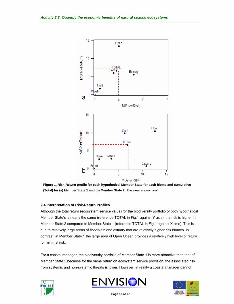
The risk-return profile for the Durham Heritage Coast (Fig. 6) illustrates that the Magnesian

Limestone biome is the biome most at risk. The actual risk value for this biome is low compared to

the other biomes (Table 10), however the profile value is as a result of a weighted calculation which

considers area and consequently the Magnesian Limestone biome has one of the largest areas. In

contrast to this, the Sand Dune biome has the greatest risk value (Table 10) but one of the smallest

areas of coverage. The profile also illustrates that the Woodland, Coastal Gills and Denes biome is

the biome that provides the most return with the Rocky Shore biome providing the least return.


of 37

0

1000

2000

3000

4000

5000

6000

0 500 1000 1500 2000 2500 3000 3500 4000 4500

Risk

Ret

urn

Figure 6. Risk-return profile for the Durham Heritage coast. a RS: Rocky Shore, SLH: Sublittoral Habitat, SD: Sand Dunes, RG: Reversion Grassland, MLG: Magnesian

Limestone Grassland, WGD, Woodland, Coastal Gills and Denes. b (Arbitrary units used)

The outcome of the Pearson’s correlation for threats (Table 11) resulted in 0 ‘Resilient’ pairs, 9

‘Independent’ pairs of biomes (Table 12) and 6 ‘Associated’ pairs of biomes (Table 13). The

Portfolio Impact Sensitivity was thus + 6, reflecting a high positive association between of the

impact of risks on biomes pairs.

Table 11. Pearson’s correlation of the threat factors for each of the biomes leads to the resultant matrix of r2 values (*) = significant; (NS) = non-significant (RS: Rocky Shore, SLH: Sub-littoral Habitat,

SD: Sand Dunes, RG: Reversion Grassland, MLG: Magnesian Limestone Grassland, WGD: Woodland,

Coastal Gills and Denes).

WGD MLG SD RG RS

MLG 0.732 (*)

SD 0.555 (NS) 0.854 (*)

RG 0.750 (*) 0.807 (*) 0.535 (NS)

RS 0.402 (NS) 0.583 (*) 0.753 (*) 0.496 (NS)

SLH -0.223

(NS)

0.047 (NS) -0.124

(NS)

-0.084

(NS)

0.147 (NS)

RS SD

RG

SLH

MLG

WGD

TOTAL


of 37

Table 12. The ‘Independent’ pairs of biomes in the biodiversity portfolio.

1. Woodland, Coastal Gills and Denes & Sand Dunes

2. Woodland, Coastal Gills and Denes & Rocky Shore

3. Woodland, Coastal Gills and Denes & Sub-littoral Habitat

4. Magnesian Limestone Grassland & Sub-littoral Habitat

5. Sand Dunes & Reversion Grassland

6. Sand Dunes & Sub-littoral Habitat

7. Reversion Grassland & Rocky Shore

8. Reversion Grassland & Sub-littoral Habitat

9. Rocky Shore & Sub-littoral Habitat

Table 13. The ‘Associated’ pairs of biomes in the biodiversity portfolio

1. Woodland, Coastal Gills and Denes & Magnesian Limestone Grassland

2. Woodland, Coastal Gills and Denes & Reversion Grassland

3. Magnesian Limestone Grassland & Sand Dunes

4. Magnesian Limestone Grassland & Reversion Grassland

7. Magnesian Limestone Grassland & Rocky Shore

8. Sand Dunes & Rocky Shore

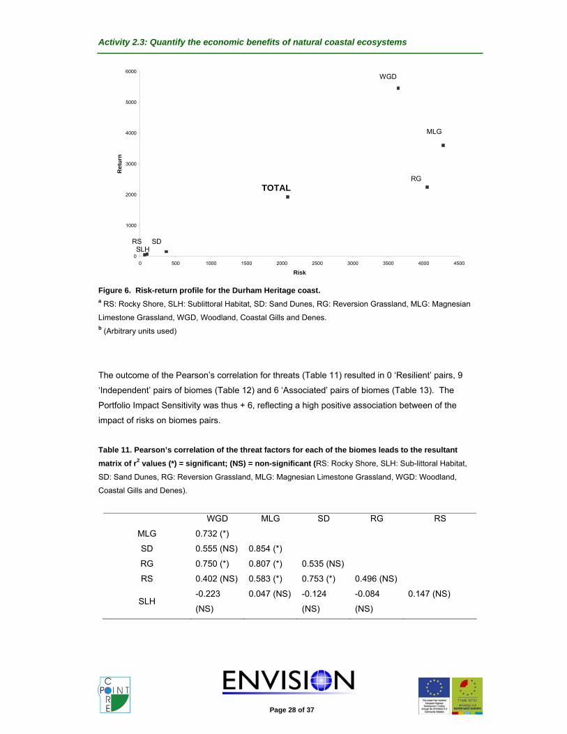
The positive association between quite a number of biomes suggests that management actions

and resources should be focused on reducing the most highly rated risks that affect all the

‘Associated’ pairs. The resulting impact that managing these particular threats would have upon

the entire portfolio (if they were managed to reduce the risk to provision of services to 0) can be

observed in the re-worked risk-return profiles (Figures 7 & 8). Fig. 7 shows the risk-return plot for

reducing the risk of recreation and tourism to 0 and Fig. 8 shows a similar plot but for reducing the

risk of recreation and tourism as well as costal erosion and sediment movement to 0. The risk to

services provided by certain biomes has been reduced and the total risk-return to the entire

biodiversity portfolio risk drops from 2082 to 1673 (Figure 8) when hypothetical management

actions are implemented simultaneously.


of 37

0

1000

2000

3000

4000

5000

6000

0 500 1000 1500 2000 2500 3000 3500 4000 4500

Risk

Ret

urn

Figure 7. Re-worked risk-return profiles showing the impact of hypothetical management strategies aimed to target and reduce the risk of tourism and recreation impact. a RS: Rocky Shore, SLH: Sub-littoral Habitat, SD: Sand Dunes, RG: Reversion Grassland, MLG: Magnesian


SD

MLG

WGD

TOTAL RG

RS SLH


of 37

0

1000

2000

3000

4000

5000

6000

0 500 1000 1500 2000 2500 3000 3500 4000

Risk

Ret

urn

Figure 8. Re-worked risk-return profile showing the impact of hypothetical management strategies aimed to reduce the risk of tourism and recreation impact and coastal erosion and sediment movement processes. a RS: Rocky Shore, SLH: Sub-littoral Habitat, SD: Sand Dunes, RG: Reversion Grassland, MLG: Magnesian


Using valid suggestions for management actions (taken from the Durham Heritage Coast

management plan), different combinations* of suggested management strategies each targeting

individual threats for individual biomes can be applied and the impact upon the risk return plot can

be determined. Three alternative management scenarios were investigated which linked into

achievement of a number of the action as identified in the Durham Heritage Coast Management

Plan. The actions which were implemented in each of the three scenarios are identified in Table 12.

The resulting risk return for each of the three scenarios can then be compared to determine the

optimal approach for management and reduction of risk to the entire portfolio (Figure 9).

TOTAL

SLH RS

SD

WGD

MLG

RG


of 37

Table 12. The actions involved in the three coastal management scenarios. The codes refer to the action

identified in the Durham Heritage Coast Plan. For each management scenario, a tick by an action means that

this action is successfully implemented.

Manag. scenarioAction code Action description

1 2 3

P1 Support regular monitoring programmes √

P2 Support and develop programmes to manage dune system √ √ √

P4 Provide advisory point for coastal development and

planning applications.

√ √

H1 Develop and support programmes to enhance protected

habitats

√ √

H2 Influence local planning processes to prevent and reduce

threats to protected landscapes and coastal habitats

√

H4 Support improvement programmes to monitor streams

flowing into coastal areas

√

H8 Develop and promote litter and pollution reducing projects √

R15 Support projects and initiatives that improve security √

S19 Support protection, management and consistency of

approach along management areas.

√

G7 Support and strengthen penalties for unauthorised use of

sites

√


of 37

0

500

1000

1500

2000

2500

0 200 400 600 800 1000 1200 1400 1600 1800 2000

Risk

Ret

urn

Figure 9. The total risk return values for the entire biodiversity portfolio of the Durham Heritage Coast when three different combinations of management strategies taken from the management plan are applied. a (Arbitrary units used) b (Combination 1 = policy recommendations P1, P2, P4 & H1. Combination 2 = policy recommendations P2,

H1, R15, G7, H8. Combination 3 = policy recommendations P2, P4, H2, H4, S19. * see p 63-93 of the

management plan for the outline of each policy recommendation or summary in Table 12.

5.4 Discussion and interpretation The risk-return profile for the Durham Heritage Coast (Figure 6) illustrates how the returns for each

biome are related to risk. The profile presents evidence that the biomes that are at the most risk

and that are affecting the sensitivity of the entire portfolio are those with large areas (Magensian

Limestone Grassland, Reversion Grassland and Woodland, Coastal Gills and Denes), even though

the actual threat factors to these biomes are relatively small compared to other biomes such as the

Sand Dune biome (Table 10). In reality a manager cannot affect the gross areas of different

habitats, but judicious management should allow threats to be managed and thus risks that

threaten the biomes to be lowered. Given that coastal managers are often faced with limited

resources, they need to know which threats should be managed in which biomes in order to lead to

the greatest reduction of risk within the risk return portfolio.

The Durham Heritage Coast case study raises an interesting issue related to reduction of overall

risk in the portfolio. The risk return analysis proposes that the risks to the most heavily weighted (by

area) biome are the key consideration to impact the overall risk of the portfolio. However, the

TOTAL

Combination 1

TOTAL

Combination 2

TOTAL

Combination 3


of 37

importance of sand-dune, which is inherently high risk but of a very small area in reducing overall

portfolio risk is minimal. The sand-dune area is however an important feature for the Durham

Heritage Coast and can be considered as a “flagship” biome nationally. Herein lays the key aspect

of the risk return approach: to reduce risks and maintain return from coastal area as a whole may

mean that relative focus on “flagship” biomes is reduced. By looking at the whole of the biome

landscape holistically, the focus in the risk return approach is on dealing with risks (especially

between associated pairs, which is a cost effective approach) to reduce overall portfolio risk and

thus maintain ecosystem service return. Viewing a coastal area as an economic generator,

concentrating on ensuring the functioning and thus economic return of the main economic

generation biomes makes sense. This however may lower the importance of “flagship” biomes

which are traditionally favoured, not for economic reasons, but for a variety of other reasons such

as biodiversity value as reflected in designations in the EU Habitats Directive. This partial

contradiction in terms of management prioritisation between economic return and maintenance of

other features, such as conservation, means that within any ICZM plan the goal needs to be

realistically stated.

On the Durham Heritage Coast, the ‘Independent’ pairs of biomes signify that even if returns from

one of the biome pairs are affected by a threat then they are not associated to returns from the

other biome pair. The ‘Associated’ pairs of biomes signify that these biomes will respond in a

similar fashion in response to threats. Due to the high level of biome pair association the portfolio

for the Durham Heritage Coast (Portfolio Impact Sensitivity = +6) lacks robustness. Clearly the

management of the coast needs to minimise risk to the associated pairs but as some of the biomes

that are independently paired are then associated to other biomes i.e. Sand Dunes & Sub-littoral

Habitat are paired independently from each other but Sand Dunes are then associated to

Magnesian Limestone Grassland and Rocky Shore, it means that the management strategies need

to be specifically targeted at individual threats. Figures 7 & 8 demonstrate how management

actions targeted at reducing tourism impact, recreation impact and erosion and sediment

movement across the whole portfolio of biomes reduces the entire portfolio risk.

The Durham Heritage Coast management plan for 2005-2010 provides comprehensive information

on the threats which are currently affecting the coastline and presents policy recommendations to

control and target these threats. The biodiversity portfolio method of valuation provides the

managers of the Durham Heritage Coast with a decision making tool which enables the managers

to consider the severity of the threats to each biome individually and also the threats that increase

risk to the entire portfolio of biomes. As a decision making tool it also enables the managers to

make choices as to which of the policy recommendations in their management plan should be

implemented with regard to minimising risk and maximising the return of individual biomes whilst

also considering the whole portfolio and reducing the overall risk. Figure 9 illustrates how

allocating ICZM resources to different combinations of policy recommendations targeting different

threats, can affect the entire risk value of the portfolio whilst still maintaining the same return.


of 37

Considering the threats table (Table 10) and the risk return profile (Figure 6), it is possible to

identify certain threats that operate at high risk across the portfolio. The highest rated threats

across the portfolio are the systemic threats of climate change and sea-level rise which

unfortunately as threat, are impossible to manage in their entirety. Nonetheless some of the

consequences of these threats can be managed.

The portfolio method of valuation is useful in this sense as it makes the coastal managers able to

strategically plan ahead for management of potential consequences of these threats for the entire

portfolio of biomes due to the awareness of the interaction between the elements within the

portfolio area. The risk return profile (Figure 6) indicated that the biomes most at risk were the

ones with large areas even thought the actual threat factors to them were not the highest when

compared with the other biomes. The weighting with area here may be misleading, as the Sand

Dune biome is highly threatened but due its small area it appears at a small risk when regarded

within the full portfolio. In spite of this seeming limitation, the biodiversity portfolio method

essentially highlights that whilst the Sand Dune may not be regarded as the biome that negates the

most risk within the portfolio, the Sand Dune biome is still a priority which, with appropriate

management of the risk will reduce the overall risk to the Durham Heritage Coast Portfolio.

The portfolio method can be used to assess the effect of management interventions through a

range of possible scenarios and thus also become a planning tool facilitating agreement between

stakeholders for optimal interventions. As described, using three different combinations of policy

recommendations for management actions (that have been outlined in the Durham Heritage Coast

management plan with the potential aim of targeting some of the threats that currently pose a

problem), it is possible to evaluate the possible outcome of these actions against the threats to the

biome and to observe the impact that these that management actions would have on the entire

portfolio (Figure 9). The combinations of policy recommendations used were selected from the

management plan to specifically target at least one more of the main threats affecting the each of

the biomes.

To carry out this study, it was essential to conduct interviews with representatives of at least half

the stakeholder groups involved with the Durham Heritage Coast. The necessity of this being to

avoid bias due to the diverse nature of interests that each of the stakeholder groups hold. The

stakeholder groups involved with the Durham Heritage Coast ranged from small local conservation

groups (for example Groundwork based in East Durham) to borough councils and even national

representative bodies such as English Nature. With this in mind, there was always going to be the

inevitable consequence that each stakeholder group as a whole and even the attitudes, opinions

and knowledge of the individual person representing the stakeholder group were going to be highly

variable. The differences that became apparent through stakeholder discussion related to the

following issues:


of 37

(i) the identification of biome types and the associated boundaries

(ii) identification and formation of a list of ecosystem services and threats relating to each biome

(iii) the rating of ecosystem services and threats for each biome.

The differences in opinions, perceptions and attitudes to the preceding issues may stem from a

lack of knowledge and understanding about a specific biome and its related services, bias towards

areas where the stakeholder group is heavily involved and failing to even consider or appreciate a

certain component of value such as bequest or option value due to lack of understanding. The

limitations that are brought about as an outcome of the differences is that the resulting total ratings

of ecosystem service provided by and threats to some biomes due to a consensus, may not be

entirely true to the Durham Heritage Coast.

5.5 Conclusions The Biodiversity portfolio method of valuation provides an effective decision making tool for use

within an ICZM framework at a local scale. Management of a portfolio can be based upon using

this tool in the decision making process to maximise return at the minimum of risk, with the

management implications being that ICZM resources should be targeted to certain biomes and it is

possible that these are not the most valuable but those that negate the most risk. Thus the

analysis of the portfolio provides an approach that doesn’t necessarily weight biomes which are

valuable irrespective of risk, but considers biomes at a landscape scale attempting to provide

highest return at the minimum of risk.


of 37

ACKNOWLEDGMENTS The authors would like to thank Dr John Firn (Firn Crichton Roberts Ltd.) for the effort retrieving the

archived data on biomes area in Members states that formed the underlying dataset for the

biodiversity portfolio analysis. The authors would also like to thank Caroline Robinson (University of

Newcastle upon Tyne) for help with the Durham Heritage Coast case study and Niall Benson

(Durham County Council) and other stakeholders from Durham Heritage Coast who took part in the

discussions on risks and returns. The authors would also like to thank the other members of the

COREPOINT team for comments and inputs into this work, especially Jeremy Gault (CMRC,

University of Cork).

coastal research and policy integration corepoint – eu ...corepoint.ucc.ie/2.3 quantification of...

Documents