classification-based music transcriptiongraham/papers/poliner_thesis_book08.pdf · abstract...
TRANSCRIPT

Classification-Based Music Transcription
Graham E. Poliner
Submitted in partial fulfillment of therequirements for the degree
of Doctor of Philosophyin the Graduate School of Arts and Sciences
COLUMBIA UNIVERSITY2008

(This page intentionally left blank)

c© 2008
Graham E. PolinerAll Rights Reserved

(This page intentionally left blank)

AbstractClassification-Based Music Transcription
Graham E. Poliner
Music transcription is the process of resolving the musical score from anaudio recording. The ability to generate an accurate transcript of a musi-cal performance has numerous practical applications ranging in nature fromcontent-based organization to musicological analysis. Although trained mu-sicians can generally perform transcription within a constrained setting, theprocess has proven to be quite challenging to automate since the recognitionof multiple simultaneous notes is generally obfuscated by the harmonic seriesinteraction that renders music aurally pleasing.
In contrast to model-based approaches that incorporate prior assumptionsof harmonic or periodic structure in the acoustic waveform, we present aclassification-based framework for automatic music transcription. The pro-posed system of support vector machine note classifiers temporally constrainedvia hidden Markov models may be cast as a general transcription framework,trained specifically for a particular instrument, or used to recognize higher-level musical concepts such as melodic sequences. Although the classificationstructure provides a simple and competitive alternative to model-based sys-tems, perhaps the most important result of this thesis is that no formal acous-tical prior knowledge is required in order to perform music transcription.
We report a series of experiments, with corresponding comparisons to alter-native approaches, in which the proposed framework is used to transcribereal-world polyphonic music ranging in diversity from ensemble orchestralrecordings to popular music tracks. In addition, we describe several meth-ods for extending a limited set of labeled training data, thereby improvingthe generalization capabilities of the classification system. Finally we relatea demonstrative experiment in which the classification posteriors (i.e. theoutputs of the proposed framework) are used as an acoustic feature represen-tation.

(This page intentionally left blank)

Contents
1 Introduction 11.1 Contributions . . . . . . . . . . . . . . . . . . . . . . . . . . . . . 2
1.2 Overview and Organization . . . . . . . . . . . . . . . . . . . . . 3
2 Background 52.1 Music Transcription . . . . . . . . . . . . . . . . . . . . . . . . . . 5
2.2 Melody Transcription . . . . . . . . . . . . . . . . . . . . . . . . . 8
2.3 Score to Audio Alignment . . . . . . . . . . . . . . . . . . . . . . 12
2.4 Summary . . . . . . . . . . . . . . . . . . . . . . . . . . . . . . . . 13
3 Melody Transcription 153.1 Audio Data . . . . . . . . . . . . . . . . . . . . . . . . . . . . . . . 15
3.1.1 Multitrack Recordings . . . . . . . . . . . . . . . . . . . . 16
3.1.2 MIDI Audio . . . . . . . . . . . . . . . . . . . . . . . . . . 16
3.1.3 Resampled Audio . . . . . . . . . . . . . . . . . . . . . . 18
3.1.4 Validation and Test Sets . . . . . . . . . . . . . . . . . . . 18
3.2 Acoustic Features . . . . . . . . . . . . . . . . . . . . . . . . . . . 19
3.3 Melody Classification . . . . . . . . . . . . . . . . . . . . . . . . . 22
3.3.1 C-way All-Versus-All SVM Classification . . . . . . . . . 22
3.3.2 Multiple One-Versus-All SVM Classification . . . . . . . 25
3.4 Voiced Frame Detection . . . . . . . . . . . . . . . . . . . . . . . 27
3.5 Hidden Markov Model Post Processing . . . . . . . . . . . . . . 28
3.5.1 HMM State Dynamics . . . . . . . . . . . . . . . . . . . . 28
3.5.2 Smoothing Discrete Classifier Outputs . . . . . . . . . . 29
3.5.3 Exploiting Classifier Posteriors . . . . . . . . . . . . . . . 29
3.6 Experimental Analysis . . . . . . . . . . . . . . . . . . . . . . . . 33
3.6.1 Evaluation Metrics . . . . . . . . . . . . . . . . . . . . . . 33
3.6.2 Empirical Results . . . . . . . . . . . . . . . . . . . . . . . 34
3.7 Summary . . . . . . . . . . . . . . . . . . . . . . . . . . . . . . . . 36
4 Polyphonic Music Transcription 374.1 Audio Data and Features . . . . . . . . . . . . . . . . . . . . . . 37
4.1.1 Audio Data . . . . . . . . . . . . . . . . . . . . . . . . . . 37
4.1.2 Acoustic Features . . . . . . . . . . . . . . . . . . . . . . . 38
4.2 Piano Note Classification . . . . . . . . . . . . . . . . . . . . . . 39
4.3 Hidden Markov Model Post Processing . . . . . . . . . . . . . . 42
4.4 Experimental Results . . . . . . . . . . . . . . . . . . . . . . . . . 43
i

4.4.1 Evaluation Metrics . . . . . . . . . . . . . . . . . . . . . . 43
4.4.2 Piano Transcription . . . . . . . . . . . . . . . . . . . . . . 45
4.4.3 Multiple Fundamental Frequency Estimation . . . . . . 48
4.5 Summary . . . . . . . . . . . . . . . . . . . . . . . . . . . . . . . . 52
5 Improving Generalization for Classification-Based Transcription 535.1 Audio Data . . . . . . . . . . . . . . . . . . . . . . . . . . . . . . . 53
5.2 Generalized Learning . . . . . . . . . . . . . . . . . . . . . . . . . 54
5.2.1 Semi-Supervised Learning . . . . . . . . . . . . . . . . . 54
5.2.2 Multiconditioning . . . . . . . . . . . . . . . . . . . . . . 55
5.3 Experiments . . . . . . . . . . . . . . . . . . . . . . . . . . . . . . 55
5.4 Summary . . . . . . . . . . . . . . . . . . . . . . . . . . . . . . . . 57
6 Score to Audio Alignment 596.1 Audio Data and Features . . . . . . . . . . . . . . . . . . . . . . 59
6.1.1 Audio Data . . . . . . . . . . . . . . . . . . . . . . . . . . 59
6.1.2 Short-Time Fourier Transform . . . . . . . . . . . . . . . 60
6.1.3 Classification Posteriors – Transcription Estimate . . . . 61
6.1.4 Peak Structure Distance . . . . . . . . . . . . . . . . . . . 61
6.1.5 Chroma . . . . . . . . . . . . . . . . . . . . . . . . . . . . 61
6.2 Time Alignment . . . . . . . . . . . . . . . . . . . . . . . . . . . . 62
6.2.1 Similarity Matrix . . . . . . . . . . . . . . . . . . . . . . . 62
6.2.2 Dynamic Time Warping . . . . . . . . . . . . . . . . . . . 62
6.3 Alignment Experiments . . . . . . . . . . . . . . . . . . . . . . . 63
6.3.1 Evaluation Metric . . . . . . . . . . . . . . . . . . . . . . . 63
6.3.2 Time Distortion . . . . . . . . . . . . . . . . . . . . . . . . 63
6.3.3 Note Deletion . . . . . . . . . . . . . . . . . . . . . . . . . 65
6.3.4 Variation in Instrumentation . . . . . . . . . . . . . . . . 65
6.4 Bootstrap Learning . . . . . . . . . . . . . . . . . . . . . . . . . . 66
6.5 Summary . . . . . . . . . . . . . . . . . . . . . . . . . . . . . . . . 67
7 Conclusion 69
Bibliography 73
ii

List of Figures
1.1 Short-time Fourier transform spectral representation . . . . . . 2
3.1 Melody transcription training data generation . . . . . . . . . . 17
3.2 Variation of melody transcription classification accuracy withthe number of training frames per excerpt . . . . . . . . . . . . 23
3.3 Variation of melody transcription classification accuracy withthe total number of training excerpts . . . . . . . . . . . . . . . . 24
3.4 Example melody transcription posteriorgram . . . . . . . . . . . 26
3.5 Melody transcription hidden Markov model parameters . . . . 32
3.6 Melody transcription error histogram comparison . . . . . . . . 35
3.7 Example melody transcription estimate comparison . . . . . . . 35
4.1 Piano transcription training and testing set note distributions . 38
4.2 Variation of piano transcription classification accuracy with thenumber of training frames per excerpt . . . . . . . . . . . . . . . 40
4.3 Variation of piano transcription classification accuracy with thetotal number of training excerpts . . . . . . . . . . . . . . . . . . 41
4.4 Example piano transcription posteriorgram and HMM estimates 42
4.5 Variation in transcription performance with the number of si-multaneous notes . . . . . . . . . . . . . . . . . . . . . . . . . . . 46
6.1 Score to audio alignment data generation and feature analysis . 60
6.2 Example similarity matrix . . . . . . . . . . . . . . . . . . . . . . 63
6.3 Score to audio alignment mean onset errors for the tempo dis-torted test set . . . . . . . . . . . . . . . . . . . . . . . . . . . . . 64
6.4 Score to audio alignment mean onset errors for the transcriptdistorted test set . . . . . . . . . . . . . . . . . . . . . . . . . . . . 65
6.5 Score to audio alignment mean onset errors for the time-scaled,transcript distorted test set . . . . . . . . . . . . . . . . . . . . . 66
7.1 Piano transcription note insertion analysis . . . . . . . . . . . . 70
iii

(This page intentionally left blank)
iv

List of Tables
2.1 Representative polyphonic transcription algorithms . . . . . . . 6
2.2 Representative melody transcription algorithms . . . . . . . . . 9
2.3 Representative score to audio alignment algorithms . . . . . . . 12
3.1 Summary of the ADC 2004 melody contest test data . . . . . . 18
3.2 Summary of the MIREX 2005 melody evaluation test data . . . 19
3.3 Acoustic feature analysis . . . . . . . . . . . . . . . . . . . . . . . 21
3.4 Impact of including resampled training data on melody tran-scription accuracy . . . . . . . . . . . . . . . . . . . . . . . . . . . 22
3.5 Impact of classification structure on melody transcription accu-racy . . . . . . . . . . . . . . . . . . . . . . . . . . . . . . . . . . . 25
3.6 Voicing detection analysis . . . . . . . . . . . . . . . . . . . . . . 27
3.7 Impact of HMM smoothing on melody transcription accuracy . 30
3.8 Results of the MIREX 2005 melody transcription evaluation . . 34
4.1 Piano transcription frame-level classification results . . . . . . . 46
4.2 Piano transcription classification accuracy comparison for syn-thesized and piano recordings . . . . . . . . . . . . . . . . . . . 47
4.3 Piano transcription classification results for the Marolt test set . 48
4.4 Piano note onset detection results . . . . . . . . . . . . . . . . . 48
4.5 Piano transcription data description . . . . . . . . . . . . . . . . 50
4.6 MIREX 2007 frame-level multiple fundamental frequency eval-uation results . . . . . . . . . . . . . . . . . . . . . . . . . . . . . 51
4.7 MIREX 2007 note-level multiple fundamental frequency evalu-ation results . . . . . . . . . . . . . . . . . . . . . . . . . . . . . . 51
5.1 Generalization experiment transcription error results . . . . . . 57
6.1 Score to audio alignment mean onset errors for the hand-labeledopera data set . . . . . . . . . . . . . . . . . . . . . . . . . . . . . 66
6.2 Bootstrap generalization experiment transcription error results 67
v

(This page intentionally left blank)
vi
Acknowledgments
Firstly, I would like to thank my advisor, Professor Dan Ellis, from whomI have learned so much more than signal processing techniques. I am pro-foundly grateful that he was willing to take an unwarranted chance on me,and I will continue to strive toward the standard he set. I cannot imagine amore erudite advisor or a mentor better suited to my disposition.
I would also like to thank Professors Juan Bello, Shih-Fu Chang, Brad Garton,and John Kymissis for serving on my Ph.D. committee and for their influentialinstruction, comments, and discussions over the past few years.
While studying in LabROSA, I have been extremely fortunate to be a partof a warm community of brilliant researchers. I am very grateful to all themembers of the group for their insights and friendship, and I am proud to beamong their peers.
Finally, I would like to thank my family: my sister Caitlin, for whom bound-aries do not exist and from whom I derive so much inspiration; Laurie Ortiz,whose love and infinite optimism have buoyed my spirits an uncountablenumber of times; and my parents, who have ensured that my wildest dreamshave all become reality and to whom I would like to dedicate this thesis.Please accept this work as a token of my appreciation for all the love andsupport you have provided me.
vii

(This page intentionally left blank)
viii

1
Chapter 1
Introduction
Music elicits a plethora of responses from listeners, and as such, has receivedresearch consideration in fields ranging from philosophy to signal processing.Recently, the pervasiveness of music data led to the establishment of an en-tirely new research arena, music information retrieval, specifically concernedwith developing methods for the organization and analysis of the rapidlygrowing musical universe. This thesis is concerned with one such method,automatic music transcription, and its application to content-based audio re-trieval.
Music transcription is the process of resolving the musical score (i.e. a sym-bolic representation) from an audio recording. Thus, transcription entailsrecovering the list of note times and pitches generated by the performer orensemble. In this thesis, transcription is specifically defined as estimating thefundamental frequency for the set of notes present within a frame of audio.
The ability to generate an accurate transcript of a performance has numerouspractical applications in content-based organization and musicological analy-sis. For example, estimated transcripts may be used to identify multiple per-formances of the same piece of music within an audio database. Alternatively,an analysis of deviations from a reference score may be used as an instructivedevice or to examine stylistic variations between a set of performances. Inaddition, an automated transcription system could be used as the front-endto a source transformation system (e.g. synthesizing an audio recording withdifferent instrumentation).
Trained musicians can typically transcribe polyphonic recordings within aconstrained setting (though the undertaking is often arduous); however, theprocess has proven to be quite challenging to automate since the recognitionof multiple simultaneous notes is generally obfuscated by the harmonic se-ries interaction that renders music aurally pleasing. While a single musicalnote may be represented by a set of harmonics at integer multiples of thefundamental frequency under Fourier analysis as displayed in the left pane

2 1.1 Contributions
freq
/ Hz
0.5 1 1.5 2 2.5 3 3.5 4 4.50
500
1000
1500
2000
2500
3000
3500
4000
time / s0.5 1 1.5 2 2.5 3 3.5 4 4.5
0
500
1000
1500
2000
2500
3000
3500
4000
Figure 1.1: Left: Short-time Fourier transform spectral representationof a monophonic clarinet recording. Right: Spectral representation of apolyphonic quintet recording.
of Figure 1.1, ensemble music may consist of multiple notes (with fundamen-tal frequencies at simple ratios) that overlap in time. The coincidence of theharmonics results in complex patterns of constructive and destructive inter-ference in a narrowband spectral analysis as displayed in the right pane ofFigure 1.1. That is, the underlying phenomena in musical harmony signifi-cantly complicate the corresponding analysis.
This thesis also considers the subject of melody transcription, a special case ofmusic transcription in which the fundamental frequency of the most salientpitch is estimated. The melody of a piece of music is the principal part of acomposition – informally, the sequence of tones that a listener might whis-tle or hum. As such, melody provides a concise and natural descriptionof music that serves as an intuitive basis for communication and retrieval(e.g. query-by-humming). Although the fundamental mechanism requiredto deploy organizational systems based on melodic content faces similar chal-lenges to general transcription systems, melody transcription systems face theadditional challenge of discriminating the predominant note from within thepolyphony.
1.1 Contributions
In this dissertation, we propose a machine learning approach to automaticmusic transcription. The proposed framework consists of a system of supportvector machine classifiers temporally constrained via hidden Markov models.The classification-based system may be generalized to perform polyphonicpitch estimation or trained specifically to recognize the predominant melody.This learning-based approach to pitch transcription stands in stark contrastto previous approaches that incorporate prior assumptions of harmonic orperiodic structure in the acoustic waveform. While the assumption that pitcharises from harmonic components is strongly grounded in musical acoustics,

1. Introduction 3
it is not strictly necessary for transcription. As such, the main contribution ofthis thesis is a demonstration of the feasibility and simplicity of a purely datadriven approach to music transcription.
In addition to the presentation of the classification-based framework and func-tional factors that influence the performance of the approach, we propose theuse of classification posteriors as features for related music information re-trieval tasks. An illustrative experiment is reported in which the classificationposteriors (i.e. estimated transcripts) are used as acoustic features to synchro-nize musical scores to audio recordings. The resulting audio-transcript pairsmay be used to bootstrap the original classification system.
In order to demonstrate the plausibility of the proposed framework, we cre-ated a corpora of labeled data for training and testing transcription systems.The labeled testing data and evaluation metrics described in this thesis wereused to organize an international evaluation of melody transcription systemsand constituted a portion of the test data used for an similar evaluation ofpolyphonic pitch estimation algorithms.
The work directly related to this thesis was reported in three journal arti-cles [26, 54, 56] and two conference proceedings [53, 55].
1.2 Overview and Organization
The remainder of the thesis is structured as follows:
In Chapter 2, we provide a background discussion on polyphonic pitch es-timation, melody transcription, and score to audio alignment, as well as asummary of previous work.
In Chapter 3, we introduce the concept of classification-based music tran-scription in the context of melody transcription. A description of the generalframework consisting of a system of support vector machines and hiddenMarkov models is presented along with a corresponding analysis of the datacollection, feature selection, and classification experiments conducted.
In Chapter 4, we extend the single-estimate classification framework describedin Chapter 3 in order to perform polyphonic pitch transcription. The pro-posed framework is presented first as a system for polyphonic piano tran-scription then generalized for instrument-independent pitch estimation.
In Chapter 5, we examine several methods based on semi-supervised learningand multiconditioning for enhancing a limited training set thereby increasingthe generalization capabilities of the proposed framework.
In Chapter 6, we explore the use of classification posteriors as acoustic fea-tures for score to audio alignment and present a keystone experiment inwhich the synchronized score/audio pairs are used to bootstrap the super-vised classification system.

4 1.2 Overview and Organization
Finally in Chapter 7, we make concluding remarks regarding the merits andlimitations of the classification-based framework and propose directions forfuture work.

5
Chapter 2
Background
In this chapter we provide background information and a discussion of priorresearch in the areas of polyphonic pitch estimation, melody transcription,and score to audio alignment. Although providing an exhaustive catalog ofprevious work is impractical, we have, to the best of our knowledge, surveyeda number of representative approaches for each of the research problems con-sidered.
2.1 Music Transcription
Music transcription is the process of resolving a musical score from an audiorecording. As such, transcription involves recovering the list of note timesand pitches generated by a performer or ensemble. In order to automate thetranscription process, a system must estimate the set of fundamental frequen-cies that correspond to the notes played within a given period of time (i.e.detecting the pitch, onset, and duration of each note).
Automated music transcription has a rich signal processing history datingback into the 1970s. In [47], Moorer proposed a limited system for duet tran-scription. Since then, a long thread of research has gradually improved tran-scription accuracy and reduced the scope of constraints (e.g. limitations onthe number of concurrent notes or confinement to a specific instrument) re-quired for successful transcription1; however, we are still far from a systemthat can automatically convert a recording into an accurate transcript in an un-constrained setting. Nonetheless, automatic music transcription has garnereda significant amount of research attention since such a system would havenumerous practical implications in musicological analysis and content-basedretrieval.
1A recent summary of the field is available in [40].

6 2.1 Music Transcription
System Front end Multi-pitch Note events Post-processingRyynanen [62] |STFT| Harmonic
sieveHMM
Smaragdis [68] |STFT| NMF – –Marolt [43] Harmonic os-
cillatorsNeural Nets Onset detection ad hoc algorithms
Kameoka [37] Power spectrum clustering via EM – –Martin [45] Auditory cor-
relogramBlackboard hypotheses heuristics
Davy [46] AR/harmonicmodel
Bayesian network –
Cemgil [8] Stochasticprocesses
Bayesian network –
Bello [2] Time domain Mixing ma-trix, phase-alignment to adatabase
– –
Table 2.1: Representative polyphonic transcription algorithms. Forbrevity, systems are referred to by their first author alone.
The algorithm structure and characteristic design parameters for a represen-tative set of (western tonal music) polyphonic pitch transcription systems isdisplayed in Table 2.1. For example, all transcription systems must select adomain in which to examine the audio signal (e.g. spectrum or time domain),adopt an approach for handling temporal overlap of simultaneous notes withdifferent periods, and may include further processing to organize frame-levelpitch estimates into structured note events. The first column of the table,“Front end”, describes the various signal processing approaches applied tothe input audio in oder to reveal the pitch content. The most common tech-nique is to apply the magnitude of the short-time Fourier transform (denoted|STFT| in the table). In the |STFT| representation, pitched notes appear asa ‘ladder’ of more-or-less stable harmonics in the spectrogram as displayedin Figure 1.1. Unlike the time waveform itself, |STFT| is invariant to relativeor absolute time or phase shifts in the harmonics because the STFT phase isdiscarded. This result is convenient since perceived pitch has essentially nodependence on the relative phase of (resolved) harmonics, and it makes thetranscription invariant to the alignment of the analysis time frames. Sincethe frequency resolution of the STFT improves with temporal window length,these systems tend to employ long windows (e.g. 50 to 100 ms or more).
As an alternative to the STFT, Martin applies the log-lag correlogram [25],which is based on the short-time autocorrelation correlogram described in [67].Like the |STFT|, the autocorrelation (which may be calculated by taking theinverse Fourier transform of the |STFT|) is phase invariant. Rather than ex-plicitly calculating a Fourier transform, Davy proposed an autoregressive-based polyphonic harmonic model in order to represent the acoustical en-ergy. Although the system proposed by Cemgil does not strictly calculate aFourier transform or implement a sinusoidal model, the signal is modeled bya stochastic process that typically results in periodic oscillations.

2. Background 7
In stark contrast to the systems discussed above, Bello does not attempt tomodel the frequency domain characteristics of the signal at all. Instead, seg-ments under consideration are phase-aligned in the time domain and tran-scription is performed via a database comparison to previously seen notes.As such the proposed time-domain implementation is necessarily restrictedto cases in which the phase relationship between partials in a given note maybe assumed to be reproducible (e.g. piano notes) and essentially limited tothe monophonic case for practical purposes due to the computational expenseof calculating and storing representative phase combinations.
Kameoka proposed harmonic temporal structured clustering (HTC), a methodwith similarities to earlier work by Goto [33], which attempts to perform thefront-end feature extraction and multi-pitch estimation cooperatively. TheHTC model decomposes the energy patterns of the power spectrum (as cal-culated using a Gabor-based wavelet transform) into clusters such that eachgroup corresponds to a single source. The sources are then modeled by amixture of two dimensional Gaussians that are constrained harmonically infrequency and continuously in time. Transcription is performed by fittingmixtures of the source models to the observed power spectrum by updatingmodel parameters and clustering the energy patterns via expectation maxi-mization (EM).
The “Multi-pitch” column of Table 2.1 addresses how the representative sys-tems deal with estimating the multiple periodicities present in the polyphonicaudio. Systems that apply the |STFT| typically perform transcription by iden-tifying the set of fundamental frequencies corresponding to the observed har-monic series. This operation is generally performed by implementing a ‘har-monic sieve’ [31, 23], which, in principle, considers each possible fundamentalby integrating evidence from every predicted harmonic location. One weak-ness of this approach is its susceptibility to reporting a spectrum one octavetoo high, since if all the harmonics of a fundamental frequency f0 are present,then the harmonics of a putative fundamental 2 f0 will also be present. Themulti-pitch identification stage of Ryynanen’s implementation [39] is essen-tially an iterative harmonic sieve; however, lower fundamentals are identifiedfirst and the spectrum is modified at each iteration in order to remove theenergy associated with the identified pitch, thereby removing evidence foroctave transpositions.
Martin performed multi-pitch detection and note event modeling simultane-ously by implementing a blackboard system [25]. The proposed frameworkincorporated knowledge ranging from the low-level correlogram features de-scribed above to hypotheses of note structure and musical rules in order toperform transcription.
The remaining representative systems perform multi-pitch estimation usingconventional machine learning techniques. In addition to many others, Smaragdisperforms polyphonic pitch estimation via non-negative matrix factorization(NMF) [41], an unsupervised learning technique popular in audio scene anal-ysis that learns harmonic structure from the magnitude spectra. In the sys-
8 2.2 Melody Transcription
tem proposed by Marolt, transcription is achieved by using neural networksto classify the outputs of adaptive harmonic oscillators. Likewise, Davy em-ploys a Bayesian framework based on Markov Chain Monte Carlo samplingof harmonic oscillator posterior distributions. Finally, the graphical modelproposed by Cemgil emulates sound generation by incorporating prior infor-mation on music structure with low-level acoustical analysis in a switchingKalman filter framework.
The “Note events” and “Post-processing” columns of Table 2.1 relate how, ifat all, the representative multiple fundamental frequency transcription sys-tems convert pitch estimates to the note-level of abstraction. Whereas Martin,Davy, and Cemgil consider notes (or at least onsets) in tandem with pitchestimation2, a number of transcription systems integrate musicological con-siderations in a separate stage. Systems such as those proposed by Maroltand Martin employ heuristics in order to incorporate a representation of mu-sical knowledge or common errors (e.g. removing octave transpositions). Incontrast, Ryynanen resolves note events with a hidden Markov model (HMM)that incorporates musicological considerations (e.g. key estimates and bigrammodels) and imposes temporal consistency on the multi-pitch estimations.
2.2 Melody Transcription
Melody transcription is a special case of music transcription that entails esti-mating the fundamental frequency of the ‘predominant pitch’ within a polyphony,loosely defined as the dominant perceived melody note. In the context ofidentifying the main melody within multi-instrument music, the music tran-scription problem is further complicated because although multiple pitchesmay be present at the same time, at most just one of them will be the melody.Thus, all approaches to melody transcription face two problems: identifyinga set of candidate pitches that appear to be present at a given time, thendiscriminating which (if any) of those pitches correspond to the melody.
For the scope of this thesis, we define melody as the single (monophonic)pitch sequence that a listener might reproduce if asked to whistle or hum apiece of polyphonic music (i.e. the sequence a listener would recognize asbeing the ‘essence’ of a piece of music). In particular, much of popular mu-sic contains a ‘lead vocal’ line, a sung contour which is typically the mostprominent source in the mixture, that listeners have no trouble distinguishingfrom the background accompaniment. However, classical orchestral musicand richly polyphonic piano compositions commonly possess a single, promi-nent melody line that can be agreed upon by most listeners. Thus, while weare in the dangerous position of setting out to quantify the performance ofautomatic systems seeking to transcribe something that is not strictly defined,there is some hope we can conduct a meaningful evaluation.
2The temporal clustering proposed by Kameoka may also be akin to note-level segmentation.

2. Background 9
System Front end Multi-pitch No.pitch
Onsetevents
Post-processing
Voicing
Dressler [21] |STFT|+sines Harmonicmodel fit
5 Fragments Streamingrules
Melody+localthresh.
Marolt [44] |STFT|+sines EM fit oftone models
> 2 Fragments Proximityrules
Melodygrouping
Goto [33] Hierarchic|STFT|+sines
EM fit oftone models
> 2 – Trackingagents
continuous
Ryynanen [63] |STFT| Harmonicsieve
2 Note on-sets
HMM Backgroundmodel
Paiva [50] Auditorycorrelogram
Summaryautocorrela-tion
> 2 Pitches Pruningrules
Melodygrouping
Vincent [76] YIN / Timewindows
Gen. modelinference
5 / 1 – HMM continuous
Table 2.2: Representative melody transcription algorithms. For brevity,systems are referred to by their first author alone.
In [35, 33], Goto proposed identifying a single, dominant periodicity over themain musical spectral range (plus a single low-frequency bass line estimate)which he referred to as “Predominant-F0 Estimation” or PreFEst. In Goto’ssystem, the predominant fundamental is generally recognizable as the melodyof the polyphonic music, and as such, the system provides a representative“sketch” of popular music. Such a representation may be used to implementa number of practical systems such as query-by-humming [30] or as a toolto analyze musicological primitives, and as a result, a great deal of researchhas recently taken place with respect to automatic melody transcription assummarized by the representative systems in Table 2.2.
The “Front end” column of Table 2.2 describes the various signal processingapproaches applied to input audio in oder to reveal the pitch content. As wasthe case for general music transcription, the most common technique is toapply the magnitude of the short-time Fourier transform. In a slightly morecomplex implementation, Goto uses a hierarchy of STFTs in order to improvefrequency resolution, down-sampling the original 16 kHz audio through 4
factor-of-2 stages resulting in a 512 ms window at the lowest (i.e. 1 kHz)sampling rate. Since musical semitones are logarithmically spaced with aratio between adjacent fundamental frequencies of 21/12 ≈ 1.06, to preservesemitone resolution down to the lower extent of the pitch range (i.e. below100 Hz) requires these longer windows. Dressler, Marolt, and Goto furtherreduce their magnitude spectra by recording only the sinusoidal frequenciesestimated as relating to prominent peaks in the spectrum, using a variety oftechniques (such as instantaneous frequency [29]) to exceed the resolution ofthe STFT bins.
A number of systems apply autocorrelation as an alternative to the STFT. Inthe representative systems listed, Paiva uses the Lyon-Slaney auditory modelup to the summary autocorrelation [67], and Vincent uses a modified version

10 2.2 Melody Transcription
of the YIN pitch tracker [18] to generate candidates for time-domain modelinference. The Lyon-Slaney model calculates autocorrelation on an approxi-mation of the auditory nerve excitation, which separates the original signalinto multiple frequency bands, then sums the normalized results. In order toperform multi-pitch detection, Paiva simply identifies the largest peaks in thesummary autocorrelation. Although YIN incorporates autocorrelation acrossthe full frequency band, Vincent performs the calculation based on the STFTrepresentation, and reports gains from some degree of across-spectrum en-ergy normalization. Interestingly, because the resolution of autocorrelation isa function of the sampling rate rather than the window length, Paiva uses asignificantly shorter window of 20 ms, and considers periods only out to 9 mslag (110 Hz).
The “Multi-pitch” column of Table 2.2 addresses how the representative sys-tems deal with distinguishing the multiple periodicities present in the poly-phonic audio, and the following column, “No. pitch”, quantifies the numberof simultaneous pitches reported at any time. Systems that apply the |STFT|transcribe the melody note by identifying the fundamental frequency of theharmonic series (even though there need not be any energy at that fundamen-tal for humans to perceive the pitch), generally performed by implementinga harmonic sieve. Ryynanen’s melody transcription implementation employsthe same iterative harmonic sieve multi-pitch stage as the polyphonic systemdescribed above.
Goto proposed an expectation maximization technique for estimating weightsover all the possible fundamentals in order to jointly explain the observedspectrum. As such, the different fundamentals effectively compete for har-monics, a process that is largely successful in resolving octave ambiguities.Marolt modified the EM procedure slightly to incorporate perceptual prin-ciples and to consider, exclusively, fundamentals that are equal to (or oneoctave below) observed frequencies. As a result, EM assigns weights to ev-ery possible pitch (most of which are very small), and the largest weightedfrequencies are taken as the potential pitches at each frame (with two to fivepitches typically considered).
Although Vincent uses autocorrelation in order to estimate up to five candi-date pitches, the core of his system is a generative model for the time-domainwaveform within each window that includes parameters for fundamental fre-quency, overall gain, amplitude envelope of the harmonics, the phase of eachharmonic, and a background noise term that scales according to local energyin a psychoacoustically-derived manner. The optimal parameters are inferredfor each candidate fundamental, and the one with the largest posterior prob-ability under the model is chosen as the melody pitch at that frame.
The “Onset events” column of Table 2.2 reflects that only some of the repre-sentative systems attempt to incorporate note (or note-series) level analysis.The systems proposed by Goto and Vincent simply estimate a single melodypitch at every frame and do not attempt to form them into higher-level note-type structures. Dressler and Marolt, however, track the amplitude variation

2. Background 11
in the harmonic sets (since there may still be multiple candidate notes) in or-der to form distinct fragments of more-or-less continuous pitch and energy.Paiva attempts to resolve the continuous pitch tracks into piecewise-constantfrequency contours, thereby removing effects such as vibrato and slides be-tween notes in order to provide a representation closer to the underlying,discrete melody sequence.
Ryynanen uses a hidden Markov model that provides distributions over fea-tures including an ‘onset strength’ related to the local temporal derivative oftotal energy associated with a pitch. The first, “attack”, state models the sharpjump in onset characteristics expected for new notes, although a bimodal dis-tribution also allows for notes that begin more smoothly; the following “sus-tain” state is able to capture the greater salience (energy), narrower frequencyspread, and lesser onset strength associated with continuing notes. Thus,new note events can be detected simply by noting transitions through the on-set state for a particular note model in the best-path (Viterbi) decoding of theHMM.
The “Post-processing” column of Table 2.2 examines how the raw (multi)pitch tracks are further refined in order to produce the final melody estimates.In the systems proposed by Dressler, Marolt, and Paiva, post-processing in-volves selecting a subset of the notes or note fragment elements to form asingle melody line, including gaps where no melody note is selected. In eachcase, the post-processing is achieved by applying sets of rules that attempt tocapture the continuity of realistic melodies in terms of energy and pitch (e.g.avoiding or deleting large, brief, frequency jumps). Rules may also includesome musical insights, such as preference for a particular pitch range, andfor the highest or lowest (outer) voices in a set of simultaneous pitches (apolyphony). Although the system proposed by Goto does not employ an in-termediate stage of note elements, it does distinguish between multiple pitchcandidates via a set of interacting “tracking agents” – alternate hypotheses ofthe current and past pitch – that compete to acquire the new pitch estimatesfrom the current frame, and that live or die based on a continuously-updatedpenalty that reflects the total strength of the past pitches they represent; thestrongest agent determines the final pitch reported.
Ryynanen and Vincent both use HMMs in order to limit the dynamics oftheir pitch estimates (i.e. to provide a degree of smoothing that favors slowly-changing pitches). Ryynanen simply connects the per-note HMMs describedabove through a third, noise/background, state, and incorporates musicologically-informed transition probabilities that vary depending on an estimate of thecurrent chord or key [74]. Vincent uses an HMM simply to smooth pitchsequences, training the transition probabilities as a function of interval sizefrom the ground-truth melodies in the 2004 evaluation set.
The “Voicing” column of Table 2.2 considers how, specifically, the systems dis-tinguish between the intervals where the melody is present and those whereit is silent (gaps between melodies). Goto and Vincent simply report theirbest pitch estimate at every frame and do not admit gaps. As discussed

12 2.3 Score to Audio Alignment
System Features Similarity SynchronizationRaphael [60] “Activity” and |STFT| HMMOrio & Schwarz [49] Peak Structure Distance DPHu et al. [36] Chroma Euclidian Distance DPTuretsky & Ellis [72] |STFT| Cosine Distance DP
Table 2.3: Representative score to audio alignment algorithms.
above, the selection of notes or fragments in the systems proposed by Dressler,Marolt, and Paiva naturally leads to gaps where no suitable element is se-lected; Dressler augments this with a local threshold to discount low-energynotes.
2.3 Score to Audio Alignment
Score to audio alignment is the process of synchronizing a symbolic repre-sentation with a recording. For many recordings, a corresponding score isavailable in the form of sheet music or a MIDI transcript. Since a recordedperformance is not an exact recreation of the score, expressive and stylisticvariations exist between different interpretations of the same piece of music.As such, developing a time mapping between the note labels and audio eventsin a given recording enables an analysis of variations between performancesand has a number of practical applications ranging from content-based in-dexing to automatic music accompaniment. We note that the basic theory ofscore to audio alignment is very similar in nature to string matching in speechrecognition [58] and biological sequence analysis [24].
In the majority of cases, score to audio alignment algorithms may be bro-ken down into three stages: acoustic feature analysis, feature similarity (ordistance) calculation, and time synchronization. Typically, a set of acousticfeatures is calculated for both the recorded audio and a synthesis of the refer-ence transcript. Then, a similarity calculation is performed by comparing thepairs of acoustic feature vectors at discrete time steps, a process that resultsin a distance matrix. Finally, time alignment is accomplished by identifyingthe least cost path through the distance matrix. Table 2.3 displays the charac-teristic attributes for several score to audio alignment systems.
Like [17, 73], Raphael [60] sought to provide a framework for automatic mu-sical accompaniment. Monophonic recordings were aligned to a referencescore by identifying the optimal sequence of local note estimates via a hiddenMarkov model. The note sequence was observed by estimating the fundamen-tal frequency of the performance in the magnitude-STFT domain, gated by anormalized energy, “activity”, measure. In contrast to the other representativeapproaches, Raphael uses a HMM to perform the time-alignment. Althoughthe HMM framework has the potential to learn sequence structure, it is di-

2. Background 13
rectly interchangeable with dynamic time warping (DTW) [58] for pairwisesequence alignment.
Whereas the remaining approaches perform feature analysis on a feature-domain realization generated from the score by some kind of synthesis, Orioand Schwarz [49] attempted to avoid employing an explicit score synthesis toachieve alignment. As such, they proposed a specialized similarity measure,the peak structure distance (PSD). For a given set of notes from the score, PSDhypothesizes the locations of associated harmonics in the spectrum (taking forexample the first 8 multiples of the expected fundamentals), then calculatesthe similarity of the observed spectral frames to the set of notes as the pro-portion of the total spectral energy that occurs within some narrow windowaround the predicted harmonics. As the actual spectrum tends towards puresets of harmonics at the correct frequencies, the similarity tends to 1. This isthen converted to a distance by subtracting the similarity estimate from 1. Asa result, the measure neatly avoids having to model the relative energies ateach harmonic.
Hu et al. [36] and Turetsky and Ellis [72] calculate acoustic features basedon the magnitude-STFT; however, Hu et al. map each bin of the fast Fouriertransform (FFT) into the corresponding chroma classes (i.e. the 12 semitoneswithin an octave) they overlap, and Turetsky and Ellis explore a number ofmagnitude-STFT feature normalizations in order to reduce the timbral depen-dency on the consistency of the synthesis. In addition, the approaches differin that Turetsky and Ellis calculate the similarity matrices based on the innerproduct (i.e. cosine distance) whereas Hu et al. apply a Euclidian distancemetric.
Identifying the least cost path through a large distance matrix can becomequite computationally expensive. As such, a number of methods have beenproposed in order to optimize the dynamic programming (DP) search suchas [20, 38].
2.4 Summary
In this chapter, we presented a background discussion and analysis of rep-resentative research pertaining to polyphonic pitch estimation, melody tran-scription, and score to audio alignment. A wide variety of approaches werereported; however a number of common themes were identified as well (e.g.the popularity of the |STFT| feature representation). In the following chap-ters, we too employ the |STFT| front-end; however, we adopt an agnosticapproach to transcription in which classifiers are left to infer whatever regu-larities may exist in the representation of training examples taken from realmusic audio recordings.

14 2.4 Summary

15
Chapter 3
Melody Transcription
In this chapter, we introduce the concept of classification-based music tran-scription in the context of melody note discrimination. Supervised classifierstrained directly from acoustic features are used to identify the predominantmelody note in a frame of audio, and the overall note sequence is smoothedvia a hidden Markov model in order to reflect the temporal consistency ofactual melodies. The training data has the single greatest influence on anyclassification system, and as such, we begin our investigation by describingthe collection and generation of the audio data. We present several acousticfeatures and normalizations for classification and make feature comparisonsbased on a baseline all-versus-all support vector machine framework. In or-der to examine the effect of classification structure on transcription accuracy,we explore different frame-level pitch classifiers and consider the problem ofdistinguishing voiced (melody) and unvoiced (accompaniment) frames. Fi-nally, we describe the addition of temporal constraints from hidden Markovmodels and provide an empirical analysis of the classification-based systemwith comparisons to alternative approaches.
3.1 Audio Data
Supervised training of a classifier requires a corpus of labeled feature vectors.In general, larger quantities of eclectic training data will give rise to moreaccurate classifiers. In the classification-based approach to transcription, then,a significant challenge becomes collecting suitable training data. Although theavailability of digital scores aligned to real recordings is very limited, there area number of alternative sources for obtaining relevant data. We investigatedusing multitrack recordings and MIDI files as training data, and we evaluatedthe proposed approach on recently developed standard test sets.

16 3.1 Audio Data
3.1.1 Multitrack Recordings
Popular music recordings are typically created by layering a number of in-dependently recorded audio tracks. In some cases, artists (or their recordcompanies) make available separate vocal and instrumental tracks as part ofa CD or 12” vinyl single release. The a capella vocal recordings can be usedto create ground truth for the melody in the full ensemble music, since a solovoice can usually be tracked at high accuracy with standard pitch trackingsystems [70, 18]. Therefore, we can construct a set of ground truth labels aslong as we can identify the temporal alignment between the solo track and thefull recording (melody plus accompaniment). Note that the a capella record-ings are only used to generate ground truth; the classifier is not trained onisolated voices since we do not expect to use it to transcribe such data.
A collection of multitrack recordings was obtained from genres such as jazz,pop, R&B, and rock. The digital recordings were read from CD, then down-sampled into monaural files at a sampling rate of 8 kHz. The 12” vinyl record-ings were converted from analog to digital mono files at a sampling rate of8 kHz. For each song, the fundamental frequency of the melody track was esti-mated using the fundamental frequency estimator in WaveSurfer, which is de-rived from ESPS’s get f0 [66]. Estimations of the fundamental frequency werecalculated at frame intervals of 10 ms and limited to the range 70–1500 Hz.
Dynamic Time Warping was used to align the a capella recordings and thefull ensemble recordings following the procedure described in [72]. Thistime alignment was smoothed and linearly interpolated in order to achieve aframe-by-frame correspondence. The alignments were manually verified andcorrected using WaveSurfer’s graphical user interface in order to ensure theintegrity of the training data. Target labels were assigned by calculating theclosest MIDI note number to the monophonic estimation. An illustration ofthe training data generation process is displayed in Figure 3.1.
The collection of multitrack recordings resulted in 12 training excerpts rang-ing in duration from 20 s to 48 s. Only the voiced portions of each excerptwere used for training (we did not attempt to include an ‘unvoiced’ class atthis stage), resulting in 226 s (i.e. 3:46) of training audio, or 22,600 frames ata 10 ms frame rate.
3.1.2 MIDI Audio
MIDI was created by the manufacturers of electronic musical instruments asa digital representation of the notes, times, and other control information re-quired to synthesize a piece of music. As such, a MIDI file amounts to adigital music score that can easily be converted into an audio rendition. Ex-tensive collections of MIDI files exist consisting of numerous transcriptionsfrom diverse genres. The MIDI training data used in the following exper-iments was composed of several frequently downloaded pop songs from

3. Melody Transcription 17
freq
/ H
zfr
eq /
Hz
0
500
1000
1500
2000
0 0.5 1 1.5 2 2.5 3 3.5 -10
-5
0
Rel
ativ
e M
elod
ic P
ower
(dB
)
time / sec
0
500
1000
1500
2000
0
10
20
30
dB
Figure 3.1: Examples from training data generation. The fundamentalfrequency of the isolated melody track (top pane) was estimated andtime-aligned to the complete audio mix (center). The fundamental fre-quency estimates (overlaid on the spectrogram), rounded to the nearestsemitone were used as target class labels. The bottom panel shows thepower of the melody voice relative to the total power of the mix (in dB);if the mix consisted only of the voice, this would be 0 dB.
http://www.findmidis.com. The training files were converted from the stan-dard MIDI file format to monaural audio files with a sampling rate of 8 kHzusing the MIDI synthesizer in Apple’s iTunes. Although completely synthe-sized (with the lead vocal line often assigned to a wind or brass voice), theresulting audio is quite rich, with a broad range of instrument timbres andproduction effects such as reverberation.
In order to identify the corresponding ground truth, the MIDI files wereparsed into data structures containing the relevant audio information (i.e.tracks, channels numbers, note events, etc), and the melody was isolated andextracted by exploiting MIDI conventions. Commonly, the lead voice in popMIDI files is stored in a monophonic track on an isolated channel. In the caseof multiple simultaneous notes in the lead track, the melody was assumed tobe the highest note present. Target labels were determined by sampling theMIDI transcript at the precise times corresponding to the analysis frames ofthe synthesized audio.
We selected five MIDI excerpts for training, each around 30 s in length. 125 s(12,500 frames) of training audio remained after we removed the unvoicedframes from the training pool.

18 3.1 Audio Data
Category Style Melody InstrumentDaisy Pop Synthesized voiceJazz Jazz SaxophoneMIDI Folk (2), Pop (2) MIDI instrumentsOpera Classical opera Male voice (2), Female voice (2)Pop Pop Male Voice
Table 3.1: Summary of the ADC 2004 melody contest test data. Eachcategory consists of 4 excerpts, each roughly 20 s in duration. The 8 seg-ments in the Daisy and MIDI categories were generated using a synthe-sized lead melody voice, and the remaining categories were generatedusing multitrack recordings.
3.1.3 Resampled Audio
When the availability of a representative training set is limited, the quantityand diversity of musical training data may be extended by resampling therecordings to effect a global pitch shift. The multitrack and MIDI record-ings were resampled at rates corresponding to symmetric semitone frequencyshifts over the chromatic scale (i.e. ±1, 2, . . . 6 semitones); the expanded train-ing set consisted of all transpositions pooled together. The ground truth labelswere shifted accordingly and linearly interpolated to maintain time alignment(because higher pitched transpositions also acquire a faster tempo). Usingthis approach, we created a smoother distribution of the training labels andreduced bias toward the specific pitches present in the training set. The clas-sification approach relies on learning separate decision boundaries for eachindividual melody note with no direct mechanism to ensure consistency be-tween similar note classes (e.g. C4 and C#4), or to improve the generalizationof one note-class by analogy with its neighbors in pitch. Using a transposition-expanded training restores some of the advantages we might expect from amore complex scheme for tying the parameters of pitchwise-adjacent notes:although the parameters for each classifier are separate, classifiers for notesthat are similar in pitch have been trained on transpositions of many of thesame original data frames. Resampling expanded the total training pool by afactor of 13 to around 456,000 frames.
3.1.4 Validation and Test Sets
Research progress benefits when a community agrees on a consistent defini-tion of their problem of interest, then goes on to define and assemble stan-dard tests and data sets. Recently, the music information retrieval communitydeveloped formal evaluations for the melody transcription problem, startingwith the Audio Description Contest at the 2004 International Conference onMusic Information Retrieval (ISMIR/ADC 2004) [32] and continuing with theMusic Information Retrieval Evaluation eXchange (MIREX) [56]. The ADC

3. Melody Transcription 19
Melody Instrument StyleHuman voice (8 f, 8 m) R&B (6), Rock (5), Dance/Pop (4), Jazz (1)Saxophone (3) JazzGuitar (3) Rock guitar soloSynthesized Piano (3) Classical
Table 3.2: Summary of the MIREX 2005 melody evaluation test data.
2004 test set for melody estimation is composed of 20 excerpts, four fromeach of five styles, each lasting 10-25 s, for a total of 366 s of test audio. Adescription of the data used in the 2004 evaluation is displayed in Table 3.1.The corresponding reference data was created by using SMSTools [6] to esti-mate the fundamental frequency of the isolated, monophonic melody trackat 5.8 ms steps. As a convention, the frames in which the main melody isunvoiced were labeled 0 Hz. The transcriptions were manually verified andcorrected using the graphical user interface in order to ensure the quality ofthe reference transcriptions. Unless otherwise noted, the ADC 2004 test setwas used as the development set in the experiments described in this chapter.
Since the ADC 2004 data was distributed after the competition, an entirelynew test set of 25 excerpts was collected for the MIREX 2005 evaluation con-sisting of 25 excerpts ranging in length from 10-40 s, providing 536 s of totaltest audio. The same audio format was used as in the 2004 evaluation; how-ever, the ground-truth melody transcriptions were generated at 10 ms steps(in order to accommodate non-frame-based approaches) using the ESPS get f0method implemented in WaveSurfer [66]. As displayed in Table 3.2, the 2005
test data was more heavily biased toward a pop-based corpora rather thanuniformly weighting the segments across a number of styles or genres as inthe 2004 evaluation. The shift in the distribution was motivated both by therelevance of commercial applications for music organization and by the avail-ability of multitrack recordings in the specified genres. Since the 2005 test setis more representative of real-world recordings, it is inherently more complexthan the preceding test set. In Section 3.6, we evaluate the classification-basedsystem on the MIREX 2005 test set and provide comparisons to a number ofalternative approaches to melody transcription.
3.2 Acoustic Features
The acoustic feature representation described in this chapter is based on theubiquitous and well-known spectrogram, which converts a sound waveforminto a distribution of energy over time and frequency. The spectrogram iscommonly displayed as a pseudo-color or grayscale image as shown in themiddle pane of Figure 3.1, and the basic acoustic features for each time-framemay be considered vertical slices through such an image. Specifically, theoriginal music recordings (melody plus accompaniment) were combined into

20 3.2 Acoustic Features
a single (mono) channel and down-sampled to 8 kHz. The short-time Fouriertransform was applied using N = 1024 point transforms (i.e. 128 ms), an N-point Hanning window, and an 80 point advance between adjacent windows(for a 10 ms hop between successive frames). Only the coefficients correspond-ing to frequencies below 2 kHz (i.e. the first 256 spectral bins) were used inthe representative feature vector.
An analysis of preprocessing schemes was made by measuring the influenceof feature normalization on a baseline classifier. A C-way, all-versus-all (AVA)algorithm for multi-class discrimination based on support vector machinestrained by sequential minimal optimization [52] as implemented in the Wekatoolkit [78] was used as the baseline pitch classifier in the acoustic featurecomparison. In this scheme, a majority vote was taken from the output of(C2 − C)/2 discriminant functions, comparing every possible pair of classes.For computational reasons, the AVA classification experiments were restrictedto a linear kernel.
Each audio frame was represented by a 256-element input vector, with C = 60classes corresponding to five-octaves of semitones from G2 to F#7. In orderto classify the dominant melodic pitch for each frame, we assume the melodynote at a given instant to be solely dependent on the normalized frequencydata below 2 kHz. For the acoustic feature analysis experiments, we furtherassume each frame to be independent of all other frames. Additional experi-ments and details regarding the classification framework will be presented inSection 3.3.
Separate AVA classification systems were trained using six different featurenormalizations. Of these, three feature sets were based on the STFT, and threewere based on the (pseudo)autocorrelation. In the first feature representation,the audio data was simply represented by the magnitude of the STFT normal-ized such that the the energy in each frame was bounded by zero and one.For the second case, the magnitudes of the spectral bins were normalized bysubtracting the mean and dividing by the standard deviation calculated ina 71-point sliding frequency window along the columns of the spectrogram.The goal of the 71-point normalization feature is to remove some of the vari-ational influence due to differences in instrumentation and context betweenthe training and testing data. For the third STFT-based normalization scheme,cube-root compression, which is commonly used as an approximation to theloudness sensitivity of the ear, was applied to the magnitude STFT in orderto make larger spectral magnitudes appear more similar.
In order to create the fourth set of features, the autocorrelation was calculatedby taking the inverse Fourier transform (IFT) of the magnitude of the STFTfor the original windowed waveform. Similarly, the fifth feature set, the cep-strum, was generated by calculating the IFT of the log-STFT-magnitude. Notethat the cepstrum also performs a sort of timbral normalization because theoverall gain and broad spectral shape are separated into the first few cepstralbins whereas periodicity appears at the higher indexes. In addition, we at-

3. Melody Transcription 21
Training dataNormalization Multitrack MIDI BothSTFT 56.4% 50.5% 62.5%71-pt norm 54.2% 46.1% 62.7%Cube root 53.3% 51.2% 62.4%Autocorr 55.8% 45.2% 62.4%Cepstrum 49.3% 45.2% 54.6%LiftCeps 55.8% 45.3% 62.3%
Table 3.3: Effect of normalization: raw pitch accuracy results on a with-held portion of the training set for each of the normalization schemesconsidered, trained on either multitrack audio alone, MIDI synthesesalone, and both data sets combined. (The size of the training sets washeld constant, so the results are not directly comparable to the otherresults reported in this chapter.)
tempted to normalize the autocorrelation-based features by liftering (scalingthe higher-order cepstral by an exponential weight).
A comparison of the raw pitch accuracy for the classifiers trained on eachof the different normalization schemes is displayed in Table 3.3. We showseparate results for the classifiers trained on multitrack audio alone, MIDIsyntheses alone, and both data sources combined. The raw pitch accuracyresults correspond to melodic pitch transcription to the nearest semitone.
The most obvious result displayed in Table 3.3 is that all the features, withthe exception of the cepstrum, result in a very similar transcription accuracy(although the across-frequency local normalization provides a slight perfor-mance advantage). This result is not altogether surprising since all the fea-tures contain largely equivalent information, but it also raises the questionas to how effective the normalization (and hence the system generalization)has been. It may be that a better normalization scheme remains to be discov-ered. Looking across the columns in the table, we see that the more realisticmultitrack data forms a better training set than the MIDI syntheses, whichhave much lower acoustic similarity to most of the evaluation excerpts. Us-ing both, and hence a more diverse training set, always gives a significantaccuracy boost – up to 9% absolute improvement, as observed for the best-performing 71-point normalized features.
The impact of including the training data transposed by resampling over ±6semitones is displayed in Table 3.4. The inclusion of the resampled data re-sults in a substantial 7.5% absolute improvement in raw pitch accuracy, aneffect that underscores the value of broadening the range of data seen foreach individual note.

22 3.3 Melody Classification
Training Set # Training Frames Raw Pitch AccNo resampling 8,500 60.2%With resampling 110,500 67.7%
Table 3.4: Impact of resampling the training data: raw pitch accuracy re-sults on the ADC 2004 test set for systems trained on the entire trainingset, either without any resampling transposition, or including transpo-sitions out to ±6 semitones (i.e 500 frames per transposed excerpt, 17
excerpts, 1 or 13 transpositions).
3.3 Melody Classification
In the previous section, we showed that classification accuracy seems to de-pend more strongly on training data diversity than on feature normalization.It may be that the SVM classifier applied in the acoustic feature analysis wasbetter able to generalize than the explicit feature normalizations. In this sec-tion, we examine the effects of different classifier types on transcription accu-racy and the influence of the total amount of training data used.
The support vector machine (SVM) [15] was selected as the learning methodto be used in the following classification experiments. The SVM is a super-vised classification system that employs a hypothesis space of linear func-tions in a high-dimensional feature space in order to learn separating hyper-planes that are maximally distant from all training patterns. As such SVMclassification attempts to generalize an optimal decision boundary betweenclasses of data. Labeled training data in a given space are thus separated bya maximum-margin hyperplane through SVM classification. Complete tutori-als and the underlying mathematical formulation for the SVM may be foundin [5, 16].
3.3.1 C-way All-Versus-All SVM Classification
Our baseline classifier is the AVA SVM as described in Section 3.2. Given thelarge amount of training data used in the evaluation (over 105 frames), weselected a linear kernel, which requires training time on the order of the num-ber of feature dimensions cubed for each of the O(C2) discriminant functions.More complex kernels (such as radial basis functions, which require trainingtime on the order of the number of instances cubed) were computationallyinfeasible due to the size of the training set.
We sought to determine the number of training instances to include from eachaudio excerpt in the first classification experiment. The number of traininginstances selected from each song was varied using both incremental sam-pling (taking a limited number of frames from the beginning of each excerpt)and random sampling (selecting the frames from anywhere in the excerpt),as displayed in Figure 3.2. Randomly sampling feature vectors to train on

3. Melody Transcription 23
0 200 60040030
35
40
45
50
55
60
65
Training samples per excerpt (17 excerpts total)
Cla
ssifi
catio
n ac
cura
cy /
%
RandomIncremental
800
Figure 3.2: Variation of classification accuracy with number of trainingframes per excerpt. Incremental sampling takes frames from the begin-ning of the excerpt; random sampling takes them from anywhere. Thetraining set does not include resampled (transposed) data.
approaches an asymptote much more rapidly than adding the data in chrono-logical order. In addition, random sampling appears to exhibit symptoms ofover-training.
The observation that random sampling achieves peak accuracy within approx-imately 400 samples per excerpt (out of a total of around 3000 samples for a30 s excerpt with 10 ms hops) may be explained by both signal processingand musicological considerations. Firstly, adjacent analysis frames are highlyoverlapped, sharing 118 ms out of a 128 ms window, and thus their featurevalues will be very highly correlated (10 ms is an unnecessarily fine timeresolution to generate training frames, but it is the standard used in the eval-uation). From a musicological point of view, musical notes typically maintainapproximately constant spectral structure over hundreds of milliseconds; anote should maintain a steady pitch for some significant fraction of a beat tobe perceived as well-tuned. If we assume there are on average 2 notes persecond (i.e. around 120 bpm) in the pop-based training data, then we expectto see approximately 60 melodic note events per 30 s excerpt. Each note maycontribute a few usefully different frames to tuning variation such as vibratoand variations in accompaniment. Thus we expect many clusters of largelyredundant frames in the training data, and random sampling down to 10%(or closer to one frame every 100 ms) seems reasonable.
The observation that analysis frames are highly overlapped also gives us a per-spective on how to judge the significance of differences in these results. Forexample, the ADC 2004 test set consists of 366 s, or 36,600 frames using thestandard 10 ms hop. A simple binomial significance test may be used to com-pare classifiers by estimating the likelihood that random sets of independenttrials could produce the observed differences in empirical error rates froman equal underlying probability of error. Since the standard error of suchan observation falls as 1/
√T for T trials, the significance interval depends

24 3.3 Melody Classification
0 20k 40k 60k 80k 100k35
40
45
50
55
60
65
70
75
Number of training frames (500 x 13 = 6500 per excerpt)
Training Data + Resampled Audio
PooledPer excerpt
Cla
ssifi
catio
n ac
cura
cy /
%
5 excerpts
10 excerpts
15 excerpts
Figure 3.3: Variation of classification raw pitch accuracy with the to-tal number of excerpts included, compared to sampling the same totalnumber of frames from all excerpts pooled. This data set includes 13
resampled versions of each excerpt, with 500 frames randomly sampledfrom each transposition.
directly on the number of trials. However, the arguments and observationsabove show that the 10 ms frames are anything but independent; to obtainsomething closer to independent trials, we should test on frames no less than100 ms apart, and 200 ms sampling (5 frames per second) would be a saferchoice. This corresponds to only 1,830 independent trials in the test set; a one-sided binomial significance test suggests that differences in frame accuracieson this test of less than 2.5% are not statistically significant at the accuraciesreported in this paper.
In the second classification experiment, we examined the incremental gainfrom adding novel training excerpts. The effect of increasing the number ofexcerpts (from one to 16) used to train the classification system on raw pitchaccuracy is displayed in Figure 3.3. In this case, each additional excerpt con-sisted of adding 500 randomly-selected frames from each of the 13 resampledtranspositions described in Section 3.1, or 6,500 frames per excerpt. Thus,the largest classifier was trained on 104k frames as compared to the approxi-mately 15k frames used to train the largest classifier in Figure 3.2. The solidcurve in Figure 3.3 displays the result of training on the same number offrames randomly drawn from the pool of the entire training set. Again, wenotice that the system trained from pool of total frames appears to reach anasymptote by 20k total frames, or fewer than 100 frames per transposed ex-cerpt. We suspect, however, that the level of this asymptote was determinedby the total number of excerpts. That is, we believe that the “per excerpt”trace will continue to climb upwards if additional novel training data wasavailable.

3. Melody Transcription 25
Classifier Kernel Raw Pitch ChromaAVA SVM Linear 67.7% 72.7%OVA SVM Linear 69.5% 74.0%OVA SVM RBF 70.7% 74.9%
Table 3.5: Raw pitch accuracy for multi-way classification systems basedon all-versus-all (AVA) and one-versus-all (OVA) structures. Accuracyresults are provided for both raw pitch transcription and chroma tran-scription (which ignores octave errors).
3.3.2 Multiple One-Versus-All SVM Classification
In addition to the C-way melody classification, 60 binary one-versus-all (OVA)SVM classifiers were trained representing each of the notes present in theresampled training set. The distance-to-classifier-boundary hyperplane mar-gins were treated as a proxy for a log-posterior probability for each of theclasses. Pseudo-posteriors (up to an arbitrary scaling power) were obtainedfrom the distance-to-classifier boundary by fitting a logistic model to the data.In the OVA framework, transcription was achieved by selecting the most prob-able class at each time frame. While OVA approaches are generally viewed asless sophisticated, [61] presents evidence that they can match the performanceof more complex multi-way classification schemes. An example ‘posterior-gram’ (note-class-versus-time image showing the posteriors of each class at agiven time step) for a pop excerpt is displayed with the ground truth labelsoverlaid in the bottom pane of Figure 3.4.
Since the number of classifiers required in the OVA framework is O(C) (ratherthan the O(C2) classifiers required for the AVA approach) it becomes compu-tationally feasible to experiment with alternative classifier kernels. The bestresult classification rates for each of the SVM systems examined are displayedin Table 3.5. Both OVA classifiers provide a marginal performance advantageover the pairwise classifier (with a slight edge favoring the OVA SVM systemthat uses an RBF kernel).

26 3.3 Melody Classification
time / s
prob
freq
/ Hz
0 1 2 3 4 5 6 7 80
200
400
600
800
1000
1200
1400
1600
1800
2000
-30
-20
-10
0
10
20
30
MID
I not
e nu
mbe
r
0 1 2 3 4 5 6 7 845
50
55
60
65
70
0.1
0.2
0.3
0.4
0.5
0.6
0.7
0.8
0.9
pop3
dB
Figure 3.4: Spectrogram and posteriorgram (pitch probabilities as afunction of time) for the first 8 s of pop music excerpt “pop3” fromthe ADC 2004 test set. The ground-truth labels, plotted on top of theposteriorgram, closely track the mode of the posteriors for the most part.However, this memoryless classifier also regularly makes hare-brainederrors that can be corrected through HMM smoothing.

3. Melody Transcription 27
Voicing Voicing Voicing VoicingClassifier Detection FA d′ Frame AccAll Voiced 100% 100% 0 85.6%Energy Threshold 88.0% 32.3% 1.63 78.4%Linear SVM 76.1% 46.4% 0.80 73.0%RBF SVM 82.6% 48.1% 0.99 78.3%
Table 3.6: Voicing detection performance. “Voicing Detection” is theproportion of voiced frames correctly labeled; “Voicing FA” is the pro-portion of unvoiced frames incorrectly labeled, so labeling all frames asvoiced scores 100% on both counts, as displayed in the first row. d′ is ameasure of a detector’s sensitivity that attempts to factor out the overallbias toward labeling any frame as voiced. “Voicing Frame Acc” is theproportion of all frames given the correct voicing label.
3.4 Voiced Frame Detection
Complete melody transcription involves not only deciding the note of frameswhere the main melody is active, but also discriminating between melodyand non-melody (accompaniment) frames. In this section, we briefly describetwo approaches for classifying instants as voiced (dominant melody present)or unvoiced (no melody present).
In the first approach we considered, voicing detection was performed by im-plementing a simple energy threshold. Spectral energy in the range 200 <f < 1800 Hz was summed for every 10 ms frame. Each energy sum valuewas normalized by the median energy in that band for the given excerpt, andinstants were classified as voiced or unvoiced by a global threshold as tunedon a small development set. Since the melody instrument is usually givena prominent level in the final musical mix, this approach is generally quitesuccessful (particularly after we have filtered out the low-frequency energy ofbass and drums).
In keeping with the classification-based approach, we also attempted to trainbinary SVM classifiers (using both linear and RBF kernels) based on the nor-malized magnitude of the STFT. The voiced melody classification statisticsare displayed in Table 3.6. Although we had hoped that the classifiers wouldlearn particular spectral cues as to the presence of the melody, the correspond-ing data shows that the simple energy threshold provides better voicing detec-tion results. However none of the voicing detectors investigated resulted in ahigher frame-level accuracy than simply labeling all the frames as voiced. Dueto the fact that the ADC 2004 test data is more than 85% voiced, any classifierthat attempts to identify unvoiced frames risks making more mislabeling mis-takes than unvoiced frames correctly detected. As such, we also report theperformance in terms of d′, a measure of a detector’s sensitivity that attemptsto factor out the overall bias toward labeling any frame as voiced (completedefinitions of the evaluation metrics are provided in Section 3.6).

28 3.5 Hidden Markov Model Post Processing
While the proposed voicing detection scheme is simple and not particularlyaccurate, it is not the main focus of the current work. The energy thresh-old enables the identification of nearly 90% of the melody-containing frames,without resorting to the crude choice of simply treating every frame as voiced.However, more sophisticated approaches to learning classifiers for tasks withhighly-skewed priors offer a promising future direction [10].
3.5 Hidden Markov Model Post Processing
The posteriorgram in Figure 3.4 clearly illustrates both the strengths andweaknesses of the classification approach to melody transcription. The suc-cess of the approach in estimating the correct melody pitch from audio data isclear in the majority of frames. However, the result also displays the obviousfault of classifying each frame independently of its neighbors: the inherenttemporal structure of music is not exploited. In this section, we attempt toincorporate the sequential structure that may be inferred from musical signalsby using hidden Markov models (HMMs) to impose temporal constraints1.
3.5.1 HMM State Dynamics
Similarly to our data driven approach to classification, we attempt to learn thetemporal structure of music directly from the training data. In the proposedframework, the HMM states correspond directly to a given melody pitch. Assuch, the state dynamics (transition matrix and class priors) can be estimatedfrom the ‘directly observed’ state sequences (i.e. the ground-truth transcrip-tions of the training set). The note class prior probabilities, generated bycounting all frame-based instances from the resampled training data, and thenote class transition matrix, generated by observing all frame-to-frame notetransitions, are displayed in Figure 3.5 (a) and (b) respectively.
Note that although some bias has been removed in the note priors by symmet-rically resampling the training data, the sparse nature of a transition matrixlearned from a limited training set is likely to generalize poorly to novel data.In an attempt to mitigate this lack of generalization, each element of the tran-sition matrix was replaced by the mean of the corresponding matrix diagonal.This generalization is equivalent to assuming that the probability of makinga transition between two pitches depends only on the interval between them(in semitones) and not on their absolute frequency. The resulting normalizedstate transition matrix is displayed in Figure 3.5 (c).
1A complete tutorial on the formulation and use of hidden Markov models is available in [57].

3. Melody Transcription 29
3.5.2 Smoothing Discrete Classifier Outputs
We can use an HMM to apply temporal smoothing even if we only considerthe labels assigned by the frame-level classifier at each stage and entirely ig-nore any information on the relatively likelihood of other labels that mighthave been available prior to the final hard decision being made by the classi-fier. If the model state at time t is given by qt, and the classifier output label isct, then the HMM will achieve temporal smoothing by finding the most likely(Viterbi) state sequence i.e. maximizing
∏t
p(ct|qt)p(qt|qt−1) (3.1)
where p(qt|qt−1) is the transition matrix estimated from the ground-truthmelody labels as described in the previous subsection. However, we stillneed p(ct|qt), the probability of seeing a particular classifier label ct given atrue pitch state qt. Since we cannot directly observe p(ct|qt), we may estimateit from the confusion matrix of classified frames (i.e. counts normalized togive p(ct, qt)) on a development corpus. For practical purposes, we reusedthe training set to generate the normalized counts. Reusing the training datamight lead to an overoptimistic belief about how well ct will reflect qt, but itwas the only reasonable option due to the limited nature of labeled data. Theraw confusion matrix normalized by columns (qt) to give the required condi-tionals is displayed in Figure 3.5 (d), and the normalized confusion matrix reg-ularized such that all elements along a given diagonal are equal is displayedin Figure 3.5 (e). Other than a small moving average, a normalization was notapplied to the zero (unvoiced) state. From the confusion (observation) ma-trix, we can see that the most frequently confused classifications are betweenmembers of the same chroma (i.e. separated by one or more octaves in pitch)and between notes with adjacent pitches (separated by one semitone).
For the total transcription problem (dominant melody transcription plus voic-ing detection), the baseline (memoryless) transcription was estimated by sim-ply gating the pitch classifier output with the binary energy threshold. If ateach instant we use the corresponding column of the observation (confusion)matrix in the Viterbi decoder dynamic-programming local-cost matrix, we canderive a smoothed state sequence that removes short, spurious excursions ofthe raw pitch labels. Despite the paucity of information obtained from theclassifier, a small, yet robust, absolute improvement of 0.9% in overall accu-racy is obtained from using this approach as displayed in Table 3.7.
3.5.3 Exploiting Classifier Posteriors
The OVA classification system was constructed in order to approximate log-posteriors for each pitch class, and we can use this detailed information toimprove the HMM decoding. Rather than guessing the local likelihood ofa particular note given a single output from the classification system, the

30 3.5 Hidden Markov Model Post Processing
Classifier Voicing Acc Raw Pitch Acc Overall AccMemoryless 85.1% 71.2% 70.7%MemlessAllVx 86.1% 76.8% 66.1%Discrete 83.6% 71.9% 71.6%Posteriors 86.2% 74.5% 73.2%PostAllVx 86.1% 79.4% 68.3%
Table 3.7: Melody transcription frame accuracy percentages for differ-ent systems with and without HMM smoothing. “Voicing Acc” is theproportion of frames whose voicing state is correctly labeled. “RawPitch Acc” is the proportion of pitched frames assigned the correct pitchlabel. “Overall Acc” is the proportion of all frames assigned both thecorrect voicing label, and, for voiced frames, the correct pitch label. Allresults are based on the one-versus-all SVM classifier using an RBF ker-nel. The “Memoryless” classifier simply takes the most likely label fromthe frame classifier after gating by the voicing detector; “MemlessAllVx”ignores the voicing detection and reports a pitch for all frames (to max-imize pitch accuracy). “Discrete” applies HMM smoothing to this labelsequence without additional information, “Posteriors” uses the pseudo-posteriors from the OVA SVM to generate observation likelihoods inthe HMM, and “PostAllVx” is the same except the unvoiced state isexcluded (by setting its frame posterior to zero).
likelihood of each note may be directly observed from each binary classifier.Thus, if the acoustic data at each time is xt, we may regard our OVA classifiersas giving us estimates of
p(qt|xt) ∝ p(xt|qt)p(qt) (3.2)
i.e. the posterior probabilities of each HMM state given the local acoustic fea-tures. Thus, by dividing each (pseudo)posterior by the prior of that note, weobtain scaled likelihoods that can be employed directly in the Viterbi searchfor the solution of Equation 3.1. The unvoiced state needs special treatment,since it is not considered by the main classifier. We attempted several ap-proaches for incorporating an estimate of the unvoiced state including decod-ing the pitch HMM with the unvoiced state excluded (setting its observationlikelihood to zero), then applying voicing decisions from a separate voicingHMM, and setting the observation posterior of the unvoiced state to 1/2± α,where α was tuned on the development (training set), which provided signif-icantly better results.
As shown in Table 3.7, using the posteriors as HMM features results in an ad-ditional absolute improvement of 1.6% total frame accuracy over using onlythe 1-best classification information. More impressively, the absolute accu-racy on the pitched frames jumps 3.3% as compared to the memoryless case,since knowing the per-note posteriors helps the HMM to avoid very unlikelynotes when it decides to stray from the one-best label assigned by the classi-fier. If we focus only on raw pitch accuracy (i.e. exclude the frames whose

3. Melody Transcription 31
ground truth is unvoiced from scoring), we can maximize pitch accuracy witha posterior-based HMM decode that excludes the unvoiced state, achievinga pitch accuracy of 79.4%, or 2.6% better than the comparable unsmoothedcase.

32 3.5 Hidden Markov Model Post Processing
40 45 50 55 60 65 70 75 80 85 900
0.05
0.1
0.15
0.2P
rior
Pro
babi
lity
Note Class (MIDI Note Number)
Class Prior
Current State
Pre
viou
s S
tate
Training Data Transition Matrix
40 50 60 70 80 90
40
50
60
70
80
90Normalized Transition Matrix
Current State
Pre
viou
s S
tate
40 50 60 70 80 90
40
50
60
70
80
90
Actual State
Pre
dict
ed S
tate
Discrete Observation Emission Matrix
40 50 60 70 80 90
40
50
60
70
80
90Normalized Observation Emission Matrix
Actual State
log prob
Pre
dict
ed S
tate
40 50 60 70 80 90
40
50
60
70
80
90
-12
-10
-8
-6
-4
-2
(a)
(b)
(d)
(c)
(e)
Figure 3.5: Hidden Markov parameters learned from the ground truthand confusion matrix data. Top (pane (a)): class priors. Middle:state transition matrix, raw (pane (b)), and regularized across all notes(pane (c)). Bottom: Observation likelihood matrix for the discrete-labelsmoothing HMM, raw (pane (d)) and regularized across notes (pane (e)).For panes (b) to (e), the state densities are displayed in the first columnand last row of each figure.

3. Melody Transcription 33
3.6 Experimental Analysis
In this section, we present the results of a full-scale melody transcription eval-uation, the MIREX melody transcription contest, that sought to provide anobjective comparison of approaches to melody transcription by developing astandardized test set and a consensus regarding evaluation metrics. The eval-uation was conducted in 2005 in association with the International Conferenceon Music Information Retrieval and repeated in 2006.
3.6.1 Evaluation Metrics
Algorithms submitted to the MIREX melody transcription contest were re-quired to estimate the fundamental frequency of the predominant melody ona regular time grid. In order to enable more detailed insight into the structureof each submitted system, participants were allowed to perform pitch estima-tion and voicing detection independently, i.e., each algorithm could give itsbest guess for a melody pitch even for frames that it reported as unvoiced.An attempt was made to evaluate the lead voice transcription at the lowestlevel of abstraction, and as such, the concept of segmenting the fundamentalfrequency predictions into notes was omitted from consideration. The metricsused in the evaluation were agreed upon by the participants in a discussionperiod prior to the algorithm submission deadline. A brief description of theevaluation metrics is provided below:
• The algorithms were ranked according to the overall transcription ac-curacy, a measure that combines the pitch transcription and voicing de-tection tasks. It is defined as the proportion of frames correctly labeledwith both raw pitch accuracy and voicing detection.
• The raw pitch accuracy is defined as the proportion of voiced framesin which the estimated fundamental frequency is within ±1/4 tone ofthe reference pitch (including the pitch estimation for frames estimatedunvoiced).
• The raw chroma accuracy is defined in the same manner as the rawpitch accuracy; however, both the estimated and reference frequenciesare mapped into a single chroma in order to forgive octave transposi-tions.
• The voicing detection rate is the proportion of frames labeled voiced inthe reference transcription that are estimated voiced by the algorithm.
• The voicing false alarm rate is the proportion of frames that are nottruly voiced that are estimated as voiced.
• The discriminability d′ is a measure of the sensitivity of a detector thatattempts to factor out the overall bias toward labeling any frame as

34 3.6 Experimental Analysis
Overall Raw Raw Voicing Voicing VoicingParticipant Accuracy Pitch Chroma Detection FA d′
Dressler 06 [21] 73.2% 77.7% 82.0% 89.3% 28.8% 1.80
Dressler 71.4% 68.1% 71.4% 81.8% 17.3% 1.85Ryynanen 06 [63] 67.9% 71.5% 75.0% 78.2% 16.5% 1.75
Ryynanen 64.3% 68.6% 74.1% 90.3% 39.5% 1.56
Poliner 06 [26] 63.0% 66.2% 70.4% 93.5% 45.1% 1.64
Poliner 61.1% 67.3% 73.4% 91.6% 42.7% 1.56
Paiva [50] 61.1% 58.5% 62.0% 68.8% 23.2% 1.22
Marolt [44] 59.5% 60.1% 67.1% 72.7% 32.4% 1.06
Sutton [69] 53.7% 56.4% 60.1% 64.5% 13.8% 1.46
Goto * [33] 49.9% 65.8% 71.8% 99.9% 99.9% 0.59
Vincent * [76] 47.9% 59.8% 67.6% 96.1% 93.7% 0.23
Brossier * [4] 31.9% 41.0% 56.1% 99.5% 98.2% 0.46
Table 3.8: Results of the MIREX Audio Melody Transcription evalua-tion. Results marked with a * are not directly comparable to the othersbecause those systems did not perform voiced/unvoiced detection. Forbrevity, systems are referred to by their first author alone.
voiced (which can move both hit rate and false alarm rate up and downin tandem). It converts the hit rate and false alarm into standard devi-ations away from the mean of an equivalent Gaussian distribution, andreports the difference between them. A larger value indicates a detec-tion scheme with better discrimination between the two classes [22].
Each algorithm was evaluated on the 25 test songs described in Table 3.2, andthe results of the evaluation are presented in the following subsection.
3.6.2 Empirical Results
The combined results of the 2005 and 2006 MIREX melody transcription eval-uations are displayed in Table 3.8. Since each research group was allowed tomake multiple submissions, only the top performing algorithm for each groupin a given year is presented. The memoryless, C-Way AVA SVM system wassubmitted to the 2005 evaluation, and a linear kernel (for computational ef-ficiency), OVA classification system with a posterior-based HMM smoothingstage was submitted in 2006.
In both the 2005 and 2006 competitions, the classification-based approachwas the third best performing melody transcription submission for each ofthe evaluation metrics considered. Comparing the proposed approach to theother submissions, we note that, although the Dressler system outperformedall other submissions, the classification-based system performed near the topbased on overall and raw pitch accuracy. As such, the classification-basedsystems appear to be one of the better approaches for generating candidatenote estimates.

3. Melody Transcription 35
-20 -10 0 10 200
10
20
30
40
Dressler
-20 -10 0 10 20
Goto
-20 -10 0 10 20
Ryynänen
-20 -10 0 10 20
Poliner
error / semitones
prop
ortio
n of
tota
l err
ors
/ %
Figure 3.6: Transcription error histograms where the relative frequencyof errors is plotted against the number of semitones deviation from thereference pitch.
0 1 2 3250
300
350
400
450Dressler
freq
uenc
y / H
z
0 1 2 3
Goto
0 1 2 3
Ryynänen
0 1 2 3
Poliner
time / s
Figure 3.7: Examples of melody transcription estimations from severalof the submitted systems as compared to the ground truth (light dots)for a 3.7 s excerpt from “Frozen” by Madonna.
We may gain additional insights into the nature of the classification approachby more closely examining the output of the proposed transcription system.Figure 3.6 displays a note error histogram for the classification-based systemas compared with a few of the top performing MIREX submissions. In starkcontrast to the other systems, the classification approach exhibits a significantnumber of adjacent note errors due to discretizing estimates to the nearestsemitone. We suspect that this result is due to the fact that the note-levelclassifiers may have more difficulty resolving acoustic effects such as vibratoand ‘mistuned’ notes. These effects are illustrated in Figure 3.7 in which anumber of example transcriptions are provided for an excerpt of “Frozen” byMadonna. Whereas algorithms that track the fundamental frequency of thelead melody voice (e.g. Dressler) follow the reference transcript quite closelyand provide a clear representation of the acoustic effects, the classification-based system, which discretizes estimates to the nearest semitone, provides arepresentation more closely associated with the note level of abstraction.
Contrasting the classification submissions year over year, we observe that, indiscordance with the classification results reported in Section 3.3.1, the AVAsystem provided a slight advantage in raw pitch accuracy as compared withthe OVA system. However, we suspect that this result is an artifact of thestatistical significance limitations of the ADC and MIREX data sets. Turningour attention to the raw chroma metric, we note that this measure indirectlyevaluates the candidate note identification stage and hints at the potential forimprovement in post processing. The HMM post-processing stage minimizes

36 3.7 Summary
the difference between the raw pitch and chroma accuracy by including amodel of the melody note transitions thereby reducing erroneous octave trans-positions. In addition, the HMM improves the voicing detection estimates byimposing temporal context on the voiced/unvoiced transitions. Thus, theHMM provided a modest improvement in overall accuracy by limiting thelocal melody steps and improving the voicing detection estimates.
3.7 Summary
In this chapter, we presented a classification approach to melody transcription.We have shown that a pure machine learning approach to melody transcrip-tion is viable and that such an approach can be successful even when basedon a modest amount of training data. Although the quality of diverse train-ing data was demonstrated to have the greatest impact on transcription accu-racy, modest improvements in performance may be obtained by implement-ing more complex classification structures and by temporally constraining theclassification estimates via hidden Markov models. The concepts formulatedherein will serve as the underpinnings for a general classification-based musictranscription framework to be investigated in the following chapters.
37
Chapter 4
Polyphonic MusicTranscription
In this chapter, we present a classification approach to polyphonic music tran-scription. Whereas melody transcription, as described in Chapter 3, consistsof estimating the single pitch corresponding to the most salient note, the poly-phonic transcription problem entails resolving multiple simultaneous notes ina given period of time. As such, we extend the C-way, one-versus-all classifica-tion system developed in Chapter 3 to transcribe the set of notes for which thepseudo-posterior probability exceeds a threshold in a given frame. We first ex-amine the complete transcription problem in the context of polyphonic pianotranscription, then we generalize the approach to an instrument agnostic mul-tiple fundamental frequency estimation framework. Similarly to Chapter 3,we begin our investigation with the description of our data collection and fea-ture analysis. Support vector machines trained on spectral features are used toclassify frame-level note instances, and the classifier estimates are temporallyconstrained via hidden Markov models. The polyphonic pitch classificationsystem is used to transcribe piano and ensemble recordings, and empiricalanalyses, as well as comparisons to alternative approaches, are presented.
4.1 Audio Data and Features
4.1.1 Audio Data
The audio data used to train and test the instrument specific piano transcrip-tion system was derived directly and indirectly from MIDI transcripts col-lected from the Classical Piano Midi Page, http://www.piano-midi.de/. The130 piece data set was randomly split into 92 training, 25 testing, and 13 val-
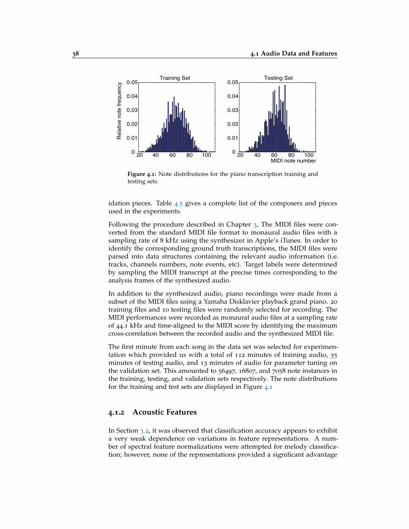
38 4.1 Audio Data and Features
20 40 60 80 1000
0.01
0.02
0.03
0.04
0.05
Rela
tive
note
freq
uenc
y
Training Set
20 40 60 80 1000
0.01
0.02
0.03
0.04
0.05
MIDI note number
Testing Set
Figure 4.1: Note distributions for the piano transcription training andtesting sets.
idation pieces. Table 4.5 gives a complete list of the composers and piecesused in the experiments.
Following the procedure described in Chapter 3, The MIDI files were con-verted from the standard MIDI file format to monaural audio files with asampling rate of 8 kHz using the synthesizer in Apple’s iTunes. In order toidentify the corresponding ground truth transcriptions, the MIDI files wereparsed into data structures containing the relevant audio information (i.e.tracks, channels numbers, note events, etc). Target labels were determinedby sampling the MIDI transcript at the precise times corresponding to theanalysis frames of the synthesized audio.
In addition to the synthesized audio, piano recordings were made from asubset of the MIDI files using a Yamaha Disklavier playback grand piano. 20
training files and 10 testing files were randomly selected for recording. TheMIDI performances were recorded as monaural audio files at a sampling rateof 44.1 kHz and time-aligned to the MIDI score by identifying the maximumcross-correlation between the recorded audio and the synthesized MIDI file.
The first minute from each song in the data set was selected for experimen-tation which provided us with a total of 112 minutes of training audio, 35
minutes of testing audio, and 13 minutes of audio for parameter tuning onthe validation set. This amounted to 56497, 16807, and 7058 note instances inthe training, testing, and validation sets respectively. The note distributionsfor the training and test sets are displayed in Figure 4.1
4.1.2 Acoustic Features
In Section 3.2, it was observed that classification accuracy appears to exhibita very weak dependence on variations in feature representations. A num-ber of spectral feature normalizations were attempted for melody classifica-tion; however, none of the representations provided a significant advantage
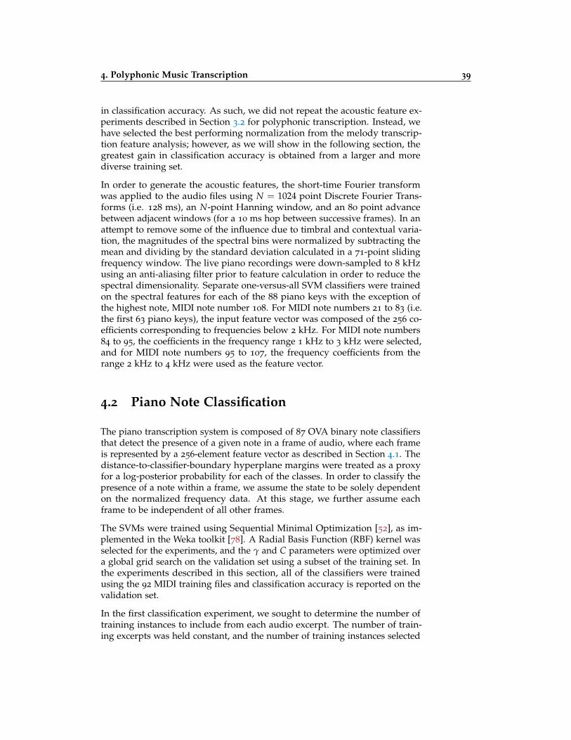
4. Polyphonic Music Transcription 39
in classification accuracy. As such, we did not repeat the acoustic feature ex-periments described in Section 3.2 for polyphonic transcription. Instead, wehave selected the best performing normalization from the melody transcrip-tion feature analysis; however, as we will show in the following section, thegreatest gain in classification accuracy is obtained from a larger and morediverse training set.
In order to generate the acoustic features, the short-time Fourier transformwas applied to the audio files using N = 1024 point Discrete Fourier Trans-forms (i.e. 128 ms), an N-point Hanning window, and an 80 point advancebetween adjacent windows (for a 10 ms hop between successive frames). In anattempt to remove some of the influence due to timbral and contextual varia-tion, the magnitudes of the spectral bins were normalized by subtracting themean and dividing by the standard deviation calculated in a 71-point slidingfrequency window. The live piano recordings were down-sampled to 8 kHzusing an anti-aliasing filter prior to feature calculation in order to reduce thespectral dimensionality. Separate one-versus-all SVM classifiers were trainedon the spectral features for each of the 88 piano keys with the exception ofthe highest note, MIDI note number 108. For MIDI note numbers 21 to 83 (i.e.the first 63 piano keys), the input feature vector was composed of the 256 co-efficients corresponding to frequencies below 2 kHz. For MIDI note numbers84 to 95, the coefficients in the frequency range 1 kHz to 3 kHz were selected,and for MIDI note numbers 95 to 107, the frequency coefficients from therange 2 kHz to 4 kHz were used as the feature vector.
4.2 Piano Note Classification
The piano transcription system is composed of 87 OVA binary note classifiersthat detect the presence of a given note in a frame of audio, where each frameis represented by a 256-element feature vector as described in Section 4.1. Thedistance-to-classifier-boundary hyperplane margins were treated as a proxyfor a log-posterior probability for each of the classes. In order to classify thepresence of a note within a frame, we assume the state to be solely dependenton the normalized frequency data. At this stage, we further assume eachframe to be independent of all other frames.
The SVMs were trained using Sequential Minimal Optimization [52], as im-plemented in the Weka toolkit [78]. A Radial Basis Function (RBF) kernel wasselected for the experiments, and the γ and C parameters were optimized overa global grid search on the validation set using a subset of the training set. Inthe experiments described in this section, all of the classifiers were trainedusing the 92 MIDI training files and classification accuracy is reported on thevalidation set.
In the first classification experiment, we sought to determine the number oftraining instances to include from each audio excerpt. The number of train-ing excerpts was held constant, and the number of training instances selected

40 4.2 Piano Note Classification
0 2k 4k 6k 8k 10k 12k 14k 16k 18k 20k40
45
50
55
60
65
70
Training instances per note class
Fram
e le
vel c
lass
ifica
tion
accu
racy
/ %
Figure 4.2: Variation of classification accuracy with number of randomlyselected training frames per note, per excerpt.
from each piece was varied by randomly sampling an equal number of pos-itive and negative instances for each note. As displayed in Figure 4.2, theclassification accuracy1 begins to approach an asymptote within a small frac-tion of the potential training data. The observation that random samplingapproaches an asymptote within a couple of hundred samples per excerpt(out of a total of 6000 for a 60 s excerpt with 10 ms hops) is consistent withand reinforces the results reported in Section 3.3.1 in which we noticed manyclusters of largely redundant training frames due to musicological and signalprocessing considerations. Since the RBF kernel requires training time on theorder of the number of training instances cubed, 100 samples per note class,per excerpt was selected as a compromise between training time and perfor-mance for the remainder of the experiments. As noted in Section 4.1, thereare an average of 8 note events per second in the training data; thus, randomsampling down to 2% (roughly equal to the median prior probability of aspecific note occurrence) is a reasonable approximation.
In the second classification experiment, we examined the incremental gain inclassification accuracy from adding novel training excerpts. In this case, thenumber of training excerpts was varied while holding the number of traininginstances per excerpt constant. Figure 4.3 shows the variation in classificationaccuracy with the addition of novel training excerpts. Each additional excerptcorresponded to 100 randomly-selected frames per note class (50 each positiveand negative instances). Thus, the largest note classifiers were trained on9200 frames. The solid curve displays the result of training on the samenumber of frames randomly drawn from the pool of the entire training set.In contrast to the effects of adding additional training excerpts described inSection 3.3 and illustrated in Figure 3.2, the two curves in Figure 4.3 are veryclosely related. This result appears to be a combined artifact of the limitedtimbral variance in MIDI piano synthesis and the fact that the piano notes are
1A detailed description of the classification metrics is provided in Section 4.4

4. Polyphonic Music Transcription 41
0 1k 2k 3k 4k 5k 6k 7k 8k 9k 10k40
45
50
55
60
65
70
Training instances per note class
Fram
e le
vel c
lass
ifica
tion
accu
racy
/ %
PooledPer excerpt
Figure 4.3: Variation of classification accuracy with the total numberof excerpts included, compared to sampling the same total number offrames from all excerpts pooled.
discretized to specific fundamental frequencies (whereas instruments such asthe human voice may vary over a bounded range). In Section 4.4.2, we beginto investigate the effect of training data generalization, a concept that becomesthe focus of Chapter 5.

42 4.3 Hidden Markov Model Post Processing
MID
I not
e nu
mbe
r
22 24 26 28 30 32 34 3640
45
50
55
60
65
70
75
time / s22 24 26 28 30 32 34 36
40
45
50
55
60
65
70
75
Figure 4.4: Top: Posteriorgram (pitch probabilities as a function of time)for an excerpt of Beethoven’s Fur Elise. Bottom: The HMM smoothedestimation (black) plotted on top of the ground truth labels (gray).
4.3 Hidden Markov Model Post Processing
Similarly to the procedure described in Section 3.5.3, we attempted to inducetemporal constraints on the independent note classifications by implementinga hidden Markov model post processing stage. Each note class was indepen-dently modeled with a two state, ‘on’/‘off’, HMM where the state dynamics(i.e. transition matrix and class priors) were estimated from the directly ob-served state sequences, the ground-truth transcriptions of the training set.Whereas the posterior-based melody transcription HMM consisted of identi-fying the single maximum likelihood sequence through the C allowed stateswhere the observation p(ct|qt) was represented by columns of the posteri-orgram, the posterior-based polyphonic HMM consists of identifying the Cmaximum likelihood binary sequences for each of the C states where theobservation p(ct|qt) is represented by the cell of the posteriorgram (and itscomplement) corresponding to the particular class under consideration.
HMM post-processing results in a 2.8% absolute improvement thus yielding aframe-level classification accuracy of 70% on the validation set. Although theimprovement in frame-level classification accuracy is relatively modest, the
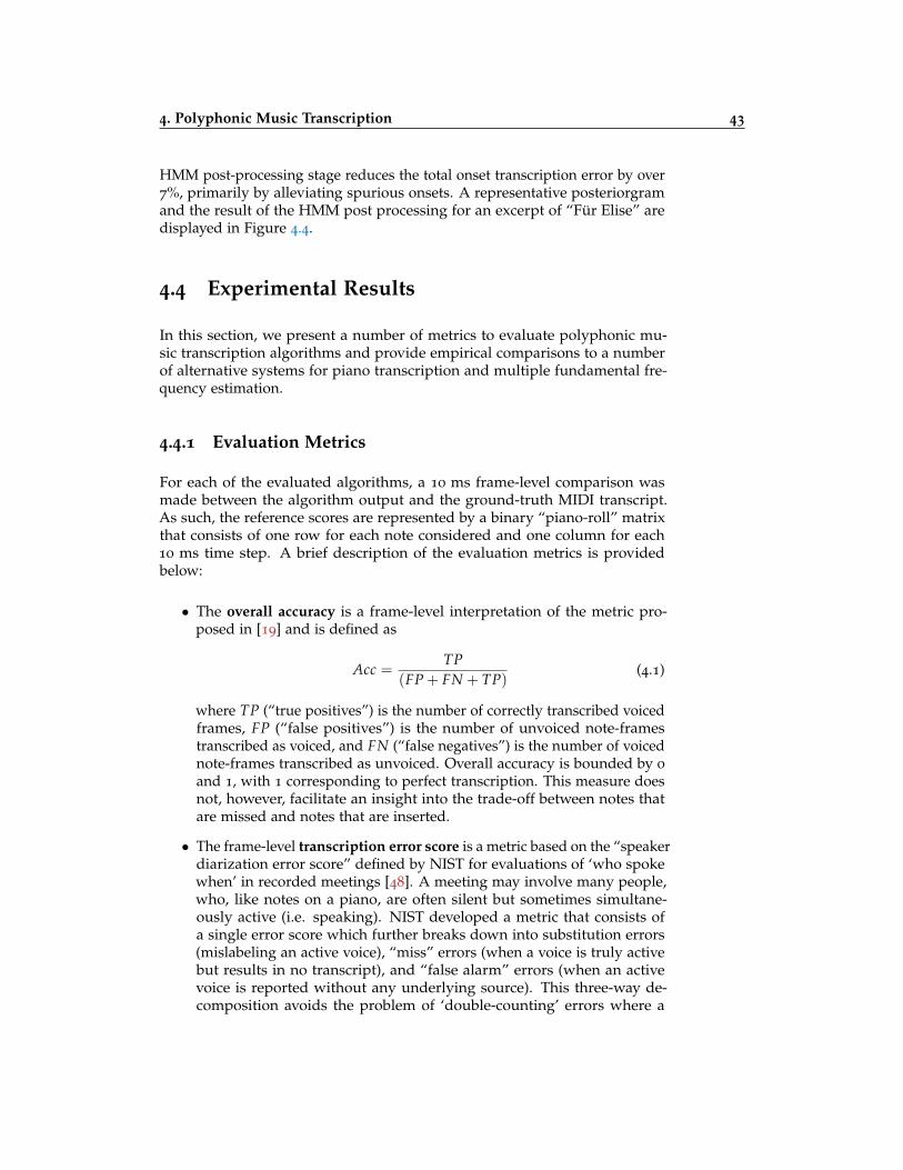
4. Polyphonic Music Transcription 43
HMM post-processing stage reduces the total onset transcription error by over7%, primarily by alleviating spurious onsets. A representative posteriorgramand the result of the HMM post processing for an excerpt of “Fur Elise” aredisplayed in Figure 4.4.
4.4 Experimental Results
In this section, we present a number of metrics to evaluate polyphonic mu-sic transcription algorithms and provide empirical comparisons to a numberof alternative systems for piano transcription and multiple fundamental fre-quency estimation.
4.4.1 Evaluation Metrics
For each of the evaluated algorithms, a 10 ms frame-level comparison wasmade between the algorithm output and the ground-truth MIDI transcript.As such, the reference scores are represented by a binary “piano-roll” matrixthat consists of one row for each note considered and one column for each10 ms time step. A brief description of the evaluation metrics is providedbelow:
• The overall accuracy is a frame-level interpretation of the metric pro-posed in [19] and is defined as
Acc =TP
(FP + FN + TP)(4.1)
where TP (“true positives”) is the number of correctly transcribed voicedframes, FP (“false positives”) is the number of unvoiced note-framestranscribed as voiced, and FN (“false negatives”) is the number of voicednote-frames transcribed as unvoiced. Overall accuracy is bounded by 0
and 1, with 1 corresponding to perfect transcription. This measure doesnot, however, facilitate an insight into the trade-off between notes thatare missed and notes that are inserted.
• The frame-level transcription error score is a metric based on the “speakerdiarization error score” defined by NIST for evaluations of ‘who spokewhen’ in recorded meetings [48]. A meeting may involve many people,who, like notes on a piano, are often silent but sometimes simultane-ously active (i.e. speaking). NIST developed a metric that consists ofa single error score which further breaks down into substitution errors(mislabeling an active voice), “miss” errors (when a voice is truly activebut results in no transcript), and “false alarm” errors (when an activevoice is reported without any underlying source). This three-way de-composition avoids the problem of ‘double-counting’ errors where a

44 4.4 Experimental Results
note is transcribed at the right time but with the wrong pitch; a simpleerror metric as used in earlier work, and implicit in Acc, biases systemstowards not reporting notes, since not detecting a note counts as a singleerror (a “miss”), but reporting an incorrect pitch counts as two errors(a “miss” plus a “false alarm”). Instead, at every time frame, the inter-section of Nsys reported pitches and Nre f ground-truth pitches countsas the number of correct pitches Ncorr; the total error score, integratedacross all time frames t is then:
Etot =∑T
t=1 max(
Nre f (t), Nsys(t))− Ncorr(t)
∑Tt=1 Nre f (t)
(4.2)
which is normalized by the total number of active note-frames in theground-truth, so that reporting no output will entail an error score of1.0. Frame-level transcription error is the sum of three components:substitution, “miss”, and “false alarm” errors.
• Substitution errors are defined as:
Esubs =∑T
t=1 min(
Nre f (t), Nsys(t))− Ncorr(t)
∑Tt=1 Nre f (t)
(4.3)
which counts, at each time frame, the number of ground-truth notes forwhich the correct transcription was not reported, yet some note was re-ported – which can thus be considered a substitution. It is not necessaryto designate which incorrect notes are substitutions, merely to count howmany there are.
• Miss errors are defined as:
Emiss =∑T
t=1 max(0, Nre f (t)− Nsys(t)
)∑T
t=1 Nre f (t)(4.4)
• False alarm errors are defined as:
E f a =∑T
t=1 max(0, Nsys(t)− Nre f (t)
)∑T
t=1 Nre f (t)(4.5)
The error equations sum, at the frame level, the number of ground-truth ref-erence notes that could not be matched with any system outputs (i.e. missesafter substitutions are accounted for) or system outputs that cannot be pairedwith any ground truth (false alarms beyond substitutions) respectively.
The error measure is a score rather than a probability or proportion i.e. itcan exceed 100% if the number of insertions (false alarms) is very high. Inline with the universal practice in the speech recognition community, we feelthis is the most useful measure since it gives a direct feel for the quantity oferrors that will occur as a proportion of the total quantity of notes present.

4. Polyphonic Music Transcription 45
It aids intuition to have the errors break down into separate, commensuratecomponents that add up to the total error, expressing the proportion of errorsfalling into the distinct categories of substitutions, misses, and false alarms.
In addition to the frame-level error metrics described above, the MIREX 2007
evaluation described in Section 4.4.3 reported note-level results using a num-ber of common signal detection metrics as well as a measure of the totalsimilarity to the reference score.
• The precision or positive predictive value is defined as:
P =TP
TP + FP(4.6)
which measures the proportion of assigned labels that were correct.
• The recall is defined as:R =
TPTP + FN
(4.7)
which measures the proportion correct labels that were assigned.
• The F1 measure combines precision and recall with equal weighting:
F1 =2PR
P + R(4.8)
in order to balance the bias towards omitting note label estimates inorder to maximize precision and including spurious note label estimatesin order to maximize recall.
• The overlap ratio as proposed in [62] is defined as:
overlap ratio =min{offsets} −max{onsets}max{offsets} −min{onsets} (4.9)
where “onsets” refers to the onset times of both the reference and es-timated note, and “offsets” refers to the onsets of the reference andestimated note.
For the note-level analysis described in Section 4.4.3, an estimated note isscored as correct if the onset is within 50 ms of the reference onset, the fun-damental frequency is within a quarter tone of the reference fundamental,and the offset value is within the larger of 20% of the duration of the note or50 ms.
4.4.2 Piano Transcription
The classification-based piano transcription system was used to estimate themusical score for the 35 (25 synthesized and 10 recorded) songs in the testing

46 4.4 Experimental Results
Algorithm Acc Etot Esubs Emiss EfaSVM [54] 65.9% 34.2% 5.3% 12.1% 16.8%Ryynanen and Klapuri [62] 46.3% 52.3% 15.0% 26.2% 11.1%Marolt [43] 36.9% 65.7% 19.3% 30.9% 15.4%
Table 4.1: Frame-level piano transcription results.
0 1 2 3 4 5 6 7 8 9
30
40
50
60
70
80
Fram
e le
vel c
lass
ificat
ion
accu
racy
/ % SVM
Klapuri&RyynanenMarolt
1 2 3 4 5 6 7 80
0.2
0.4
0.6
0.8
1
Notes present per frameTo
tal e
rror s
core missed notes
false alarmssubstitutions
Figure 4.5: Left:Variation of classification accuracy with number of notespresent in a given frame and relative note frequency. Right: Error scorecomposition as a function of the number of notes present.
set, and the results of the frame-level evaluation are displayed in Table 4.1.In addition, direct comparisons are provided to the systems proposed in [62]and [43]. We note that the Ryynanen and Klapuri system was developed forgeneral music transcription, and the parameters have not been tuned specifi-cally for piano recordings.
As displayed in Table 4.1, the classification system provides a significant per-formance advantage on the test set with respect to frame-level accuracy andthe error scores – outperforming the other two systems on 33 out of the 35
test pieces. Since the transcription problem becomes more complex as thenumber of simultaneous notes increases, we have also plotted the frame-levelclassification accuracy versus the number of notes present for each of the algo-rithms in the left panel of Figure 4.5; the total error score (broken down intothe three components) with the number of simultaneously occurring notes forthe proposed algorithm is displayed in the right panel. As expected, there isan inverse relationship between the number of notes present and the propor-tional contribution of false alarm errors to the total error score. However, theperformance degradation is not as severe for the proposed method as it is forthe comparison systems.
In Table 4.2, a breakdown of the transcription results is reported betweenthe synthesized audio and piano recordings. The proposed system exhibitsthe most significant disparity in performance between the synthesized audioand piano recordings; however, we suspect that this is because the greatest

4. Polyphonic Music Transcription 47
Algorithm Piano (10) Synthesized (25) Both (35)SVM (Piano Only) 59.2% 23.2% 33.5%SVM (MIDI Only) 33.0% 74.6% 62.7%SVM (MIDI & Piano) 56.5% 70.0% 65.9%Ryynanen and Klapuri 42.2% 47.9% 46.3%Marolt 35.4% 37.5% 36.9%
Table 4.2: Classification accuracy comparison for the MIDI test files andlive recordings. The MIDI SVM classifier was trained on the 92 MIDItraining excerpts, and the Piano SVM classifier was trained on the 20
piano recordings.
proportion of the training data was generated using synthesized audio. In ad-dition, Table 4.2 displays the classification accuracy results for SVMs trainedon MIDI data and piano recordings alone. The specific data distributions per-form well on more similar data, but generalize poorly to unfamiliar audio.These results clearly indicate that the implementations based only on onetype of training data are over-trained to the specific timbral characteristics ofthat data and may provide an explanation for the poor performance of neuralnetwork-based system. However, the inclusion of both types of training datadoes not come at a significant cost to classification accuracy for either type.As such, it is likely that the proposed system may be generalized to differenttypes of piano recordings when trained on a diverse set of training instances.
In order to investigate the generalization assumption further, the proposedsystem was used to transcribe the test set prepared by Marolt in [43]. Thisset consists of six recordings from the same piano and recording conditionsused to train his neural network and is different from any of the data in ourtraining set. The classification results on the Marolt test set are displayed inTable 4.3. The SVM system commits a greater number of substitution andmiss errors compared to its performance on the relevant portion of our testset, reinforcing the possibility of improving the stability and robustness of theSVM with a broader training set. Marolt’s classifier, trained on data closer tohis test set than to ours, outperforms the SVM here on the overall accuracymetric, although interestingly with a much greater number of false alarmsthan the SVM (compensated for by many fewer misses). The system proposedby Ryynanen and Klapuri outperforms the classification-based approacheson the Marolt test set; a result that underscores the need for a diverse setof training recordings for a practical implementation of a classification-basedapproach.
Frame-level accuracy is a particularly exacting metric. Although offset esti-mation is essential in generating accurate transcriptions, it is likely of lesserperceptual importance than accurate onset detection. In addition, the prob-lem of offset detection is obscured by relative energy decay and pedalingeffects. In order to account for these effects and to reduce the influence ofnote duration on the performance results, we report an evaluation of note

48 4.4 Experimental Results
Algorithm / test set Acc Etot Esubs Emiss EfaSVM / our piano 56.5% 46.7% 10.2% 15.9% 20.5%SVM / Marolt piano 44.6% 60.1% 14.4% 25.5% 20.1%Marolt / Marolt piano 46.4% 66.1% 15.8% 13.2% 37.1%Ryynanen and Klapuri /Marolt piano
50.4% 52.2% 12.8% 21.1% 18.3%
Table 4.3: Frame-level transcription results on recorded piano only(ours and the Marolt test sets).
Algorithm Acc Etot Esubs Emiss EfaSVM 69.1% 43.2% 4.5% 16.4% 22.4%Ryynanen and Klapuri 60.2% 46.0% 6.2% 25.3% 14.4%Marolt 33.6% 87.5% 13.9% 41.9% 31.7%
Table 4.4: Piano note onset detection results.
onset detection. A note onset was labeled as correct if the estimated onsetwas within 100 ms of the ground-truth onset. The systems were scored on themetrics described above with respect to note onsets rather than frame-leveltranscription accuracy, and the note onset transcription results are reportedin Table 4.4. When scoring the systems, substitutions were counted first byassociating unattached system outputs and ground-truth notes. Even with-out a formal onset detection stage, the proposed algorithm provides a slightadvantage over the comparison systems on the 35 song test set.
4.4.3 Multiple Fundamental Frequency Estimation
In 2007, the music information retrieval community conducted a multiple fun-damental frequency estimation evaluation as part of MIREX 2007
2. Like themelody transcription evaluations that preceded it, the goal of the multiplefundamental frequency evaluation was to provide a unified set of test dataand evaluation metrics for the community of researchers working on auto-mated transcription. For the frame-level analysis, the 28 song test set againstwhich the algorithms were evaluated consisted of 20 ensemble pieces (withvarious combinations of woodwind, brass, and string instruments) and eightsynthesized recordings from the real world computing (RWC) database [34].The ground-truth transcriptions for the 20 ensemble pieces were generatedusing a procedure similar to that described in Section 3.1.1. The results ofthe frame-level multiple fundamental frequency evaluation are presented inTable 4.6.
2http://www.music-ir.org/mirex/2007/index.php/Multiple Fundamental Frequency
Estimation & Tracking Results
4. Polyphonic Music Transcription 49
In this experiment, the piano specific classification system was generalized inorder to perform instrument-independent music transcription. The classification-based submission to the multiple fundamental frequency evaluation was trainedon the pop-based melody transcription training data3 described in Section 3.1,the piano transcription training data described in Section 4.1, and 20 ad-ditional synthesized MIDI files with varying instrumentation. In order tomaximize efficiency in classification time, linear kernel SVM classifiers weretrained for each of the C classes corresponding to the first 87 piano notes. Atwo state HMM, as described in Section 4.3, was used to temporally constrainthe classification posteriors based on the state dynamics observed in the train-ing data. Despite the fact that the data used to train the classification systembore little resemblance to the 20 ensemble pieces, the SVM-based approach tomusic transcription performed relatively well as compared to the other sub-missions finishing 6th out of 12 research groups on the total frame-level errorscore.
In addition to the frame-level evaluation, an analysis of note-level transcrip-tion systems was performed on a set of 30 recordings. The note-level test setconsisted of 16 ensemble recordings, eight synthesized recordings from theRWC database, and six piano recordings selected from the test set describedin Section 4.1. Seven of the participants attempted to formulate the funda-mental frequency estimates into notes, and the results of the note-level tran-scription analysis are displayed in Table 4.7. The note-level classifiers, whichdiscretize the fundamental frequency estimates to the nearest semitone, per-formed near the top of the evaluation as a result of operating on the notelevel of abstraction. The proposed system likely received an advantage onthe six piano test cases that were created in the same recording environmentas a fraction of the training data; however, the SVM approach was able togeneralize to a number of unseen instruments and recording environmentsrepresented in the remaining testing cases.
3Only positive training instances were selected from the melody transcription training datasince we could not exclude the possibility of a positive accompanying note instance for any giventraining frames.

50 4.4 Experimental Results
Composer Training Testing ValidationAlbeniz Espana (Prelude†, Malaguena,
Sereneta, Zortzico) SuiteEspanola (Granada, Cataluna,Sevilla, Cadiz, Aragon,Castilla)
Espana (Tango), SuiteEspanola (Cuba)
Espana (Capri-cho Catalan)
Bach Well-Tempered Clavier 1: Pre-lude & Fugue No. 5
Well-Tempered Clavier 1:Prelude & Fugue No. 2
Well-TemperedClavier 1: Pre-lude & FugueNo. 1
Balakirew Islamej†Beethoven Appassionata 1-3, Moonlight
(1, 3), Pathetique (1)†, Wald-stein (1-3)
Fur Elise† Moonlight (2),Pathetique (3)†
Pathetique (2)
Borodin Petite Suite (In themonastery†, Intermezzo,Mazurka, Serenade, Noc-turne)
Petite Suite (Mazurka) Reverie
Brahms Fantasia (2†, 5), Rhapsodie Fantasia (6)†Burgmueller The pearls†, Thunderstorm The FountainChopin Opus 7 (1†, 2), Opus 25 (4),
Opus 28 (2, 6, 10, 22), Opus 33
(2, 4)
Opus 10 (1)†, Opus 28 (13) Opus 28 (3)
Debussy Suite bergamasque(Passepied†, Prelude)
Menuet Clair de Lune
Granados Danzas Espanolas (Oriental†,Zarabanda)
Danzas Espanolas (Vil-lanesca)
Grieg Opus 12 (3), Opus 43 (4), Opus71 (3)†
Opus 65 (Wedding) Opus 54 (3)
Haydn Sonata in G major 1† Sonata in G major 2 †Liszt Grandes Etudes de Paganini
(1†-5)Love Dreams (3) Grandes Etudes
de Paganini (6)Mendelssohn Opus 30 (1)†, Opus 62 (3,4) Opus 62 (5) Opus 53 (5)Mozart Sonata in C Major (1†-3),
Sonata in B Flat Major (3)Sonata in B Flat Major (1)† Sonata in B Flat
Major (2)Mussorgsky Pictures at an Exhibition
(1†,3,5-8)Pictures at an Exhibition(2,4)
Schubert Sonata in A Minor (1†,2), Fan-tasy in C Major (1-3), Sonata inB Flat (1,3)
Fantasy in C Major (4)† Sonata in B Flat(2)
Schumann Scenes from Childhood (1-3, 5,6†)
Scenes from Childhood (4)†
Opus 1 (1)
Tchaikovsky The Seasons (February, March,April†, May, August Septem-ber, October, November, De-cember)
The Seasons (January†,June)
The Seasons(July)
Table 4.5: MIDI compositions from http://www.piano-midi.de/. †denotes songs for which piano recordings were made.

4. Polyphonic Music Transcription 51
Algorithm Etot Esubs Emiss Efa AccPertusa [51] 44.5% 9.4% 29.8% 5.3% 58.0%Yeh [79] 46.0% 10.8% 23.8% 11.5% 58.9%Ryynanen [62] 47.4% 15.8% 13.3% 18.3% 60.5%Zhou [80] 49.8% 14.1% 19.7% 16.0% 58.2%Vincent [75] 53.8% 13.5% 24.0% 16.3% 54.3%Poliner 63.9% 12.0% 37.5% 14.4% 44.4%Leveau [42] 63.9% 15.1% 43.2% 5.5% 39.4%Raczynski [59] 67.0% 18.5% 21.9% 26.5% 48.4%Cao [7] 68.5% 20.0% 12.8% 35.6% 51.0%Emiya [28] 95.7% 7.0% 76.7% 12.0% 14.5%Cont [12] 99.0% 34.8% 22.1% 42.1% 31.1%Egashira [37] 118.8% 40.1% 5.2% 73.4% 33.6%
Table 4.6: MIREX 2007 frame-level multiple fundamental frequencyevaluation results. For brevity, systems are referred to by their firstauthors alone.
Algorithm Precision Recall F1 OverlapRyynanen 0.312 0.382 0.337 0.884
Poliner 0.305 0.278 0.277 0.879
Pertusa 0.206 0.262 0.226 0.844
Vincent 0.162 0.277 0.204 0.859
Egashira 0.071 0.130 0.09 0.847
Emiya 0.098 0.052 0.076 0.804
Cont 0.015 0.044 0.023 0.831
Table 4.7: MIREX 2007 note-level multiple fundamental frequency eval-uation results.

52 4.5 Summary
4.5 Summary
In this chapter, we presented a classification approach to music transcription.We have shown that a data driven approach may be used to classify the notesof a specific instrument or generalized to an instrument agnostic transcrip-tion framework. We observed that the relevance of the training data hadthe single greatest impact on classification accuracy; however, representativetraining data is often limited. As such, we seek to investigate methods forimproving classification generalization and extending a limited training setin the following chapter.

53
Chapter 5
Improving Generalization forClassification-BasedTranscription
In this chapter, we present methods to improve the generalization capabilitiesof the classification-based approach to music transcription. Although the sys-tem proposed in Chapter 4 compared favorably with model-based approacheswhen both the training and testing recordings were made from the same setof pianos, the classification-based system exhibited a performance degrada-tion when presented with piano recordings made under different conditions.As described in the preceding chapters, classifier performance is limited bythe amount and diversity of the labeled training data available; however, agreat deal of relevant, yet unlabeled, audio data exists. In this chapter, weseek to exploit the vast pool of unlabeled data and to improve the value ofthe limited labeled data. To that end, we investigate semi-supervised learningand multiconditioning techniques for improving generalization.
5.1 Audio Data
The 92 synthesized MIDI files and 20 piano recordings described in Section 4.1were used as the labeled training data in the generalization experiments. Thevalidation set used to tune classifier parameters was collected from the RWCdatabase [34], and the ground-truth transcripts for the three validation fileswere aligned by Cont [11] following the method described in [38]. The gen-eralization test set consisted of 19 piano recordings made from three differ-ent pianos including six pieces from the test set generated by Marolt [43],two pieces created by Scheirer [64], and 11 pieces recorded on a Roland HP

54 5.2 Generalized Learning
330e digital piano downloaded from the Classical Piano Midi Page1. In caseswhere limitations in the MIDI file parsing resulted in a linear scaling betweenthe labels and test audio, a compensating scaling constant was estimated tomaximize the alignment between the reference score and a noisy transcriptionof the audio made by the baseline SVM system. In addition to the labeledaudio, 54 unlabeled polyphonic piano files were collected from 20 differentrecording environments to be used as training data in the semi-supervisedlearning experiments.
5.2 Generalized Learning
Although the classification-based system performs well on different record-ings made from the same set of pianos in the same recording environments,the success of the transcription system does not translate as well to novelpianos and unseen recording settings. In this section, we propose methodsfor improving generalization by learning from unlabeled training data and byaugmenting the value of the data for which training labels are available.
5.2.1 Semi-Supervised Learning
Millions of music recordings exist, yet only a very small fraction of them arelabeled with corresponding transcriptions. Since the success of the proposedtranscription system is so heavily dependent on the quantity and diversity ofthe available training data, we have attempted to incorporate more of the dataavailable to train new classification systems by applying different techniquesto assign labels to unlabeled data.
Nearest neighbor clustering is a simple classification system in which a labelis assigned to a particular point in the feature space based on its proximity,using a given distance metric, to its k-nearest neighbors. For each frame-levelfeature vector2 in the unlabeled data set, a set of 87 binary labels was gener-ated by calculating the Euclidian distance to each point in the training datafor a given note class and assigning the label of the (majority vote of the)k-nearest neighbors to the unlabeled point. For each note, an equal num-ber of positive and negative training instances generated from the unlabeleddata was added to the original training data set, and a new system of SVMclassifiers was trained.
In our semi-supervised SVM approach, labels were assigned to unlabeleddata by classifying the unlabeled points with our baseline SVM system. Al-though formal semi-supervised support vector machine methods have beenproposed for minimizing the structural risk by calculating the misclassifica-tion error for each unlabeled feature vector (i.e. minimizing the additional
1http://www.piano-midi.de/2The acoustic features were calculated following the procedure described in Section 4.1.2.
5. Improving Generalization for Classification-Based Transcription 55
risk of adding the data point as a positive or negative training instance) [3],classifying the unlabeled data using the framework described in Chapter 4
enables the incorporation of temporal constraints. As an alternative to usingthe raw classifier output as a proxy for training sample selection, the HMMpost-processing stage described in Section 4.3 may be applied to the outputof the unlabeled data classification. In some cases, the inclusion of the HMMstage results in class assignment updates due to temporal context, thus im-proving the insight of the trained classifier in ambiguous situations. Again,for each note, an equal number of positive and negative training instancesgenerated from the unlabeled data was added to the original training set inorder to create an updated system of classifiers.
5.2.2 Multiconditioning
The quantity and diversity of the training data was extended by resamplingthe audio to effect a global pitch shift. Each recording from the trainingset was resampled at rates corresponding to frequency shifts of a fractionof a semitone in order to account for differences in piano tunings. The cor-responding ground-truth labels were unaffected (since the target note classremained the same); however, the time axis was linearly interpolated in or-der to adjust for the resulting time scaling. Symmetrically shifted frequencydata was added to the original training set in order to create additional clas-sifiers. As such, this method for extending the training data corresponds to asub-semitone version of the resampling approach described in Section 3.1.
5.3 Experiments
In the first semi-supervised learning experiment, each frame of audio in theunlabeled data set was assigned the label of its k-nearest neighbors. Fromeach song in the unlabeled set and for each note in the classification system, 50
negative training instances and 50 positive training instances (when available)were added to the original set of training data This addition increased thequantity of training data by approximately 50%. The amount of training dataused was held constant while the number of nearest neighbors, k, was variedfrom 1 to 7 in odd increments. A classification system of SVMs was trainedfrom each of the updated training sets; however, each resulted in a negligiblechange in transcription error on the validation set.
The baseline SVM system was then used to estimate transcriptions for eachsong in the unlabeled data set. Positive training instances were selected byvarying the range of the distance to classifier boundary used for samplingselection. While holding the 50% increase in training data constant, we at-tempted sampling from a series of ranges by performing a grid search overthe distance to classifier boundary, the best of which resulted in a 0.8 pointdecrease in total error score for the validation set. In addition to sampling

56 5.3 Experiments
different distance to classifier ranges to generate training instances, the HMMpost-processing stage was applied to the raw classifier transcriptions of theunlabeled data set. From each song, 50 positive and negative instances wereselected for each note class and additional classifiers were trained resultingin an 1.1 point reduction in the total error on the validation set. In orderto demonstrate the variation in classifier performance due to the additionof semi-supervised training instances, the amount of estimated training datawas varied as a fraction of percent increase in total data from 10-100% (in10% increments) resulting in a monotonically decreasing reduction in the to-tal error score on the validation set up to 1.9 points for the training instancesgenerated from the output of the SVM classifier with HMM smoothing.
Four additional classifiers were trained in order to investigate the effects ofgenerating training data from resampled audio. Each recording from thetraining set was resampled at symmetric rates corresponding to ± 0.5, 1.0,1.5, 2.0% deviations from the original tone (where a full semitone shift corre-sponds to a ≈ 6% deviation). In this experiment, the amount of resampledtraining data was held constant, while the range of resampled audio used totrain the classifiers was varied. Incorporating the resampled audio resultedin 3.1, 1.2, 1.1, and 0.9 point reductions, respectively, in frame-level errorscore for the validation set. We suspect that the resampling rates closer tothe original tone provide an advantage in performance because they are morelikely to be in line with mild instrument de-tuning. The top performing re-sampled classifier was then used to generate labels for the unlabeled dataset. The transcriptions were temporally smoothed via the HMM, and the es-timated labels were sampled (50 positive and negative instances per class) tocreate additional training data for a final set of classifiers. The combinationof the semi-supervised learning with the resampling technique resulted in a4.7 point improvement in total error score on the validation set.
The parameters for each of the generalization techniques were optimized onthe validation set by minimizing the frame-level transcription error score, andthe top performing classification system from each of the proposed frame-works was used to transcribe the 19 songs in the test set. The correspondingframe-level transcription results are displayed in Table 5.1. The top perform-ing system, a combination of the semi-supervised and multiconditioning tech-niques, provided a 10 point reduction in total frame-level error score on thetest set.
Finally, both the baseline system and the system combining training data frommulticonditioning and semi-supervised learning were used to transcribe the10 test piano recordings described in Section 4.1. Including the diversifyingtraining data resulted in a mild 0.4 point performance degradation in totalerror score for the original instruments; however, the 10 point improvementin generalization on the novel test set seems to warrant the addition.

5. Improving Generalization for Classification-Based Transcription 57
Frame-level transcriptionSystem Etot Esubs Emiss EfaSVM (baseline) 69.7% 15.8% 36.3% 17.6%k-NN 70.5% 15.1% 37.3% 18.1%SVM 68.9% 10.2% 49.7% 9.0%SVM + HMM 68.5% 15.6% 33.9% 19.0%MC 63.0% 12.4% 39.5% 11.1%MC + SVM + HMM 59.1% 8.6% 38.6% 12.3%
Table 5.1: Generalization experiment transcription error results for the19 song test set. The systems reported correspond to methods for creat-ing additional training data.
5.4 Summary
In this chapter, we presented a number of methods for improving classifica-tion generalization for piano transcription. We have shown that a reductionin total transcription error may be achieved by combining multiconditioningand semi-supervised learning in order to generate additional training datafor a classification-based music transcription system. The proposed meth-ods demonstrate that limited quantities of training data may be augmentedin order to reduce classification error. In the following chapter, we investi-gate these concepts further by examining the effects of using classificationposteriors as alignment features in order to facilitate bootstrap learning fordeveloping training data and improving transcription accuracy.

58 5.4 Summary

59
Chapter 6
Score to Audio Alignment
In this chapter, we present a method for score to audio alignment based onsynchronizing an estimated transcript with a reference score. The frameworkdescribed in the preceding chapters is used to transcribe polyphonic audiorecordings, and the classification posteriors are synchronized to a MIDI tran-script by dynamic time warping. A key advantage of the proposed methodfor score to audio alignment is that the time-alignment is performed in thescore domain and, as such, does not require an artificial synthesis of the score.We describe a novel method for generating test cases based on leveraging asmall amount of aligned data by systematically distorting the reference score,and we report empirical comparisons to a number of alternative alignment ap-proaches. Finally, we present a keystone experiment in which the proposedmethod for score to audio alignment is used to develop a semi-supervisedclassification system for music transcription.
6.1 Audio Data and Features
6.1.1 Audio Data
The typical method for evaluating score to audio alignment approaches in-volves hand-labeling the time mapping between a recording and the corre-sponding score for a small test set. In the typical case, the audio recording isconsidered a distorted version of the target reference score. Rather than lim-iting our evaluation to a small set of hand-labeled test files, we examined theconverse approach of generating a reference recording directly from a tran-script, then distorting the reference transcript by a known warping to createmisaligned pairs of scores and recordings. In this complementary case, therecordings (and the transcripts used to generate them) are considered the ref-erence, and we attempt to map the distorted scores onto the time axis of thereference recordings. This alternative method allows us to employ a larger

60 6.1 Audio Data and Features
Reference MIDI
Recorded Audio
Synthesized Audio
Feature Analysis
DTW
MIDI to WAV
Playback piano
t
WarpingFunction
r
t (t )r wt (t )w r
^
Warped MIDI
STFT
chroma
STFT
chroma
posteriors
Transcriptionclassifier
MIDI score
tw
Figure 6.1: Flow chart of the data generation and feature analysis forscore to audio alignment.
test set (potentially including a large number of distortions) without requir-ing a large number of recordings, since each recording is aligned to multiple,distorted, scores. Consequently, the statistical quality of our analyses areimproved, and the time required for test set development is significantly re-duced.
The experimental audio data was derived from the 10 piano recording/MIDItranscript pairs described in Section 4.1. We attempted to account for typi-cal deviations that might be expected between scores and recordings whengenerating the test cases. Therefore, the reference MIDI files were distortedby varying the local tempo and by modifying the notes present in the ref-erence transcript. A complete description of the experimental distortions isprovided in Section 6.3. Figure 6.1 displays the development of the test dataand time-warping analysis.
In addition to the set of piano recordings and distorted MIDI files, we com-piled a small set of operetta songs from the 1993 D’Oyly Carte recording ofGilbert and Sullivan’s Mikado and the corresponding MIDI karaoke files fromThe Gilbert and Sullivan Archive, http://math.boisestate.edu/gas/. Thebeginning of each line of lyrics was hand labeled for the recordings and readdirectly from the karaoke file transcripts.
6.1.2 Short-Time Fourier Transform
The magnitude short-time Fourier transform was used as our baseline align-ment feature. The piano recordings and synthesized MIDI files were re-sampled to 8 kHz, and the STFT was applied to the audio files using 1024 pointdiscrete Fourier transforms (i.e. 128 ms), a 1024 point Hanning window, andan 80 point advance between adjacent windows (for a 10 ms hop between

6. Score to Audio Alignment 61
successive frames). The frequency coefficients below 2 kHz (i.e. the first256 spectral bins) were used as the features in the calculation of the similaritymatrix as described in Section 6.2.
6.1.3 Classification Posteriors – Transcription Estimate
The posterior features were calculated using the piano transcription systemdescribed in Chapter 4 (without the HMM post-processing stage) trained onthe generalized data described in Chapter 5. As in Chapter 5, linear kernelSVMs were used in order to maximize classification efficiency. The systemof SVM classifiers was used to detect the presence or absence of each notein a frame of audio, a process that resulted in an estimated transcript foreach recording. The transcript estimations were limited to the first 63 pianonotes (i.e. notes with a fundamental frequency less than 2 kHz) when calcu-lating the similarity between the warped MIDI transcript and the estimatedreference transcript.
6.1.4 Peak Structure Distance
Like us, the authors of [49] wished to avoid having to employ an explicitsynthesized audio version of their score to achieve alignment. Their solutionwas to define a specialized similarity measure, the Peak Structure Distance(PSD). For a given set of notes from the score, PSD hypothesizes the loca-tions of associated harmonics in the spectrum (taking for example the first 8
multiples of the expected fundamentals), then calculates the similarity of theobserved spectral frames to the set of notes as the proportion of the total spec-tral energy that occurs within some narrow window around the predictedharmonics. As the actual spectrum tends towards pure sets of harmonics atthe correct frequencies, the similarity tends to 1. This is then converted to adistance by subtracting the similarity metric from 1. Thus, the measure neatlyavoids having to model the relative energies at each harmonic.
6.1.5 Chroma
Chroma features attempt to capture the dominant note as well as the broadharmonic accompaniment by folding all spectral information into the 12 semi-tones within an octave. Rather than using a coarse mapping of FFT bins tothe chroma classes they overlap (which is particularly blurry at low frequen-cies), the phase-derivative (instantaneous frequency) within each FFT bin wasused both to identify strong tonal components in the spectrum (indicated byspectrally-adjacent bins with close instantaneous frequencies) and to improvethe resolution of the underlying frequency estimate [9, 1]. The chroma wasgenerated on a 10 ms grid from the spectral components below 1 kHz.

62 6.2 Time Alignment
In addition to calculating the chroma features from the synthesized MIDI files,we attempted to estimate chroma directly from the MIDI transcript. Referencepower curves, created by varying the ‘velocity’ of individual piano notes andmeasuring the power versus time, were used to approximate the relative loud-ness and decay of each note. In order to calculate the chroma features directlyfrom the notes in the MIDI file, the corresponding reference power was addedto the feature matrix rather than using a binary representation of each note inthe transcript.
6.2 Time Alignment
6.2.1 Similarity Matrix
In order to calculate the similarity between two feature matrices, we tookthe normalized inner product or cosine distance. The similarity matrix M iscalculated by:
M =AT B
ETAEB
(6.1)
where A is the feature matrix for the reference audio recording (one columnper time step) and B is the feature matrix for the time-warped recording in ouranalysis. EA and EB are row vectors containing the norms of each column ofA and B respectively, and the division is applied elementwise. The elementsof the resulting matrix M are bounded by 0 and 1, where a cell value of 1
indicates a region of high similarity between the cells of the feature matrices.
6.2.2 Dynamic Time Warping
Dynamic time warping was used to identify the least-cost time-alignmentpath through each similarity matrix. The least-cost path p is computed it-eratively via dynamic programming by minimizing the cost function for thedistance matrix, D = 1− M:
p(i, j) = min
p(i − 1, j − 1) + D(i, j)p(i − 1, j) + D(i, j)p(i, j − 1) + D(i, j)
(6.2)
An example similarity matrix and the corresponding least-cost path is dis-played in Figure 6.2. A complete treatment of DTW for audio alignment isavailable in [58].

6. Score to Audio Alignment 63
warped transcript / s
refe
renc
e / s
0 5 10 15 20 25 30 350
5
10
15
20
25
Figure 6.2: Similarity matrix calculated between an audio recording anda MIDI rendition of Tchaikovsky’s January: At the Fireside from TheSeasons. Dark regions indicate similarity between the feature matrices,and the least-cost path warping estimate is overlaid in white.
6.3 Alignment Experiments
6.3.1 Evaluation Metric
We assess the success of each of the feature representations considered byevaluating the timing error between the reference transcript and the estimatedalignment. We report the average onset timing error which is defined as themean of the timing error, errk = |tre f
k − testk |, for each note onset k in the
reference transcript. This metric is similar to the “average offset” reported in[49] and the “error” score described in [13].
6.3.2 Time Distortion
The tempo of the reference transcript was varied in order to account for lo-cal deviations (e.g. stylistic performance differences) and global shifts (e.g.playing the song more slowly). A Brownian walk W(t) was applied to thereference tempo in order to generate the warped time tw as a function ofreference time tr
W(t) = W(t − 1) + N(0, σ2) (6.3)
tw(tr) =tr
∑t=0
exp{
B · log(2) · W(t)maxτ |W(τ)|
}(6.4)
where B is a warp bound varied between 0.1 to 1. Thus, the warped time tw isobtained as the sum of a sequence of time steps that can individually vary be-tween 0.5 and 2.0 for the largest warp bound. 10 random walk iterations wereperformed for each warp bound resulting in 1000 time-warped MIDI and au-

64 6.3 Alignment Experiments
0 0.1 0.2 0.3 0.4 0.5 0.6 0.7 0.8 0.9 10
10
20
30
40
50
60
70
80
90
100
Brownian bound B
note
ons
et e
rror /
ms
STFT
posteriorsPSD
chroma
Figure 6.3: Time warp mean onset errors.
dio recording pairs. The resulting mean onset error evaluated on a 10 ms gridfor each of the features considered is displayed in Figure 6.3. Although notdisplayed in Figure 6.3, the chroma features generated directly from the MIDItranscript result in an approximate 40 ms performance degradation as com-pared to the chroma calculated from the synthesized MIDI. Chroma featuresgive relatively poor temporal alignment compared to STFT1, but PSD and pos-terior features are significantly better, with posteriors achieving a slight edgefor more drastic distortions.
Each of the comparison systems operates by making some kind of predictionof the spectrum from the score, then comparing with the actual signal in thespectral domain. The key advantage of using a classifier to generate score-likenote posteriors appears to lie in its ability to generalize across all the differentspectral realizations that a particular pitch may take. Synthetic audio derivedfrom MIDI makes a single guess about the anticipated spectra of each note,and to the extent this fails to match the actual notes observed, the similaritymatrix is compromised and alignment will suffer. The classifier, by contrast,has been trained on multiple instances of each note’s spectra, and will mapany of these versions to the same transcribed event. This result is most clearlyillustrated in the substantial improvement between alignment based on STFTfeatures and that using posteriors. The PSD, which also is able to accepta note regardless of its precise harmonic spectrum, performed comparablyto posterior matching in our tests; however, posterior feature matching wassuperior in most cases.
1A single song containing a number of arpeggios contributed disproportionately to the totalerror for the Chroma features. This test case highlights the conspicuous weakness of foldingthe observations into a single octave representation; however, the chroma features provide atheoretical advantage when the recorded audio is played in a different octave than the score.

6. Score to Audio Alignment 65
0 10 20 30 40 50 60 70 80 900
50
100
150
200
250
300
350
400
450
500
note deletion percentage / %
note
ons
et e
rror /
ms
STFT
posteriorsPSD
chroma
Figure 6.4: Note deletion mean onset errors.
6.3.3 Note Deletion
A portion of the notes present in the reference transcript were removed inorder to account for variations in performance (e.g. misplayed or spuriousnotes). Uniform random sampling was used to delete a fraction of the noteswhile holding the original tempo of the reference transcript constant. For eachfraction of notes deleted, 10 files were created resulting in 900 additional testcases. The results of the mean note onset error calculation for varying notedeletion percentages are displayed in Figure 6.4.
Both the PSD and posterior features appear to gain an advantage from thedynamic programming bias towards jointly advancing a step in each timeaxis. As such, the note deletion experiment was repeated for those two fea-tures with a constant, linear time-scaling in the distorted transcripts whileholding the specific notes deleted fixed. The test cases were scaled such thatthe distorted transcripts were 50% longer in duration, and the results of thesupplemental note deletion experiment are displayed in Figure 6.5. The poste-rior features still resulted in note onset errors of approximately 100 ms or lesswhen up to 50% of the notes were deleted from the linearly scaled transcript.
6.3.4 Variation in Instrumentation
In order to account for variations in instrumentation and synthesis qualitybetween a MIDI transcript and an audio recording, a set of eight operettarecordings, for which the symphonic MIDI representation differed from therecorded audio, were hand labeled at the beginning of each line of lyrics.These instants were selected since hand-labeling every note onset is imprac-tical for an opera recording and because the practical task of voice detec-tion facilitates vocal performance analysis such as an examination of vowel-

66 6.4 Bootstrap Learning
0 10 20 30 40 50 60 70 80 900
50
100
150
200
250
300
350
400
450
500
note deletion percentage / %
note
ons
et e
rror /
ms
posteriorsPSD
Figure 6.5: Note deletion mean onset errors for the linearly scaled testcases.
Feature ¯err (ms) ¯err (frames)STFT 324 1.62
Posteriors 316 1.58PSD 322 1.61
Chroma 375 1.87
Table 6.1: Error results for the hand-labeled opera recordings.
modification. The start times for each line of lyrics were labeled on a 100 msgrid, but the error evaluation between the recorded audio and karaoke tran-script was performed on a 200 ms grid in order to account for inaccuracies inthe hand-labeling. The mean onset error results for the hand-labeled data setare displayed in Table 6.1. In this experiment, the classification-based featureswere generated using the instrument agnostic classification system describedin Section 4.4.3.
We suspect that the hop size used in the evaluation may be a limiting factor inthe mean note onset errors (especially for the opera experiments). However,the average time alignment errors were limited to a small number of framesin the feature representation for the majority of cases.
6.4 Bootstrap Learning
The proposed method for score to audio alignment was used to synchronize46 MIDI transcripts from the data set described in Section 3.1 to piano record-ings made in a number of different recording environments (i.e. differentstudio, piano, performer, etc.) for which an exact transcript was unavailable.The note labels from the time-aligned score were associated with frames from
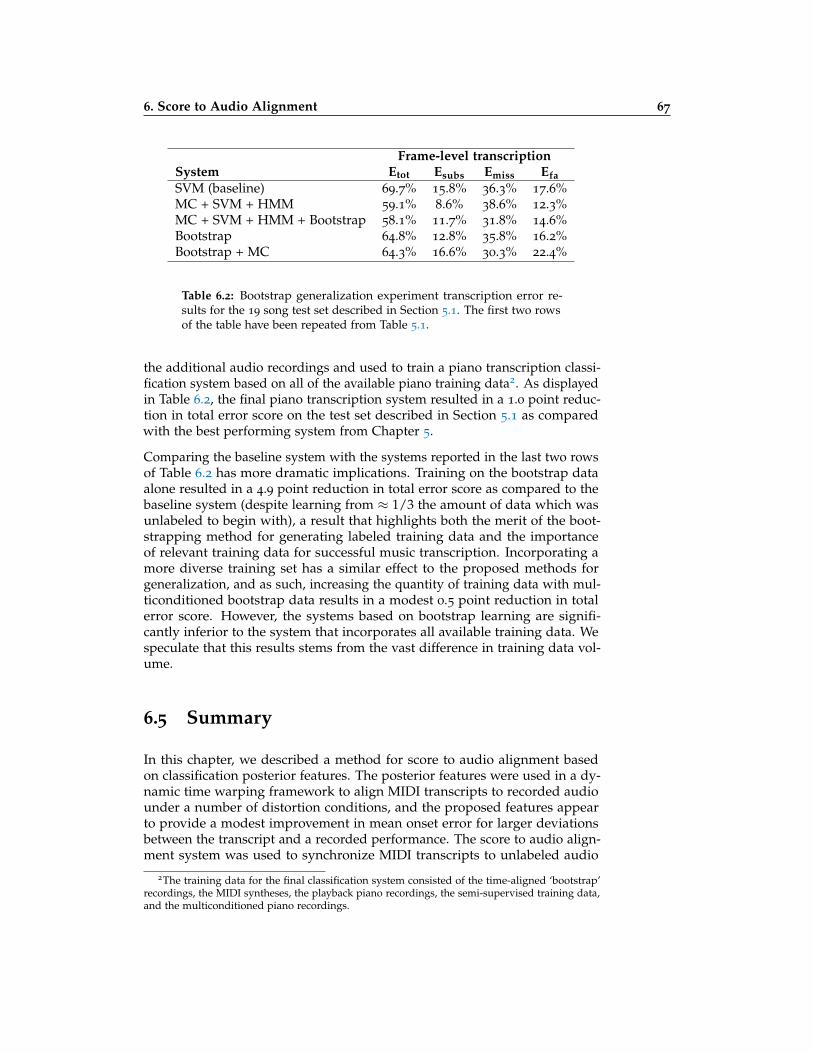
6. Score to Audio Alignment 67
Frame-level transcriptionSystem Etot Esubs Emiss EfaSVM (baseline) 69.7% 15.8% 36.3% 17.6%MC + SVM + HMM 59.1% 8.6% 38.6% 12.3%MC + SVM + HMM + Bootstrap 58.1% 11.7% 31.8% 14.6%Bootstrap 64.8% 12.8% 35.8% 16.2%Bootstrap + MC 64.3% 16.6% 30.3% 22.4%
Table 6.2: Bootstrap generalization experiment transcription error re-sults for the 19 song test set described in Section 5.1. The first two rowsof the table have been repeated from Table 5.1.
the additional audio recordings and used to train a piano transcription classi-fication system based on all of the available piano training data2. As displayedin Table 6.2, the final piano transcription system resulted in a 1.0 point reduc-tion in total error score on the test set described in Section 5.1 as comparedwith the best performing system from Chapter 5.
Comparing the baseline system with the systems reported in the last two rowsof Table 6.2 has more dramatic implications. Training on the bootstrap dataalone resulted in a 4.9 point reduction in total error score as compared to thebaseline system (despite learning from ≈ 1/3 the amount of data which wasunlabeled to begin with), a result that highlights both the merit of the boot-strapping method for generating labeled training data and the importanceof relevant training data for successful music transcription. Incorporating amore diverse training set has a similar effect to the proposed methods forgeneralization, and as such, increasing the quantity of training data with mul-ticonditioned bootstrap data results in a modest 0.5 point reduction in totalerror score. However, the systems based on bootstrap learning are signifi-cantly inferior to the system that incorporates all available training data. Wespeculate that this results stems from the vast difference in training data vol-ume.
6.5 Summary
In this chapter, we described a method for score to audio alignment basedon classification posterior features. The posterior features were used in a dy-namic time warping framework to align MIDI transcripts to recorded audiounder a number of distortion conditions, and the proposed features appearto provide a modest improvement in mean onset error for larger deviationsbetween the transcript and a recorded performance. The score to audio align-ment system was used to synchronize MIDI transcripts to unlabeled audio
2The training data for the final classification system consisted of the time-aligned ‘bootstrap’recordings, the MIDI syntheses, the playback piano recordings, the semi-supervised training data,and the multiconditioned piano recordings.

68 6.5 Summary
recordings in order to facilitate bootstrap learning, a process that resulted inan improvement in classification generalization.

69
Chapter 7
Conclusion
We have presented a classification-based approach for automatic music tran-scription. The proposed system of support vector machine note classifierstemporally constrained via hidden Markov models may be cast as a generaltranscription framework, trained specifically for a particular instrument, orused to recognize higher-level musical concepts such as melodic sequences.Although the classification structure provides a simple and competitive al-ternative to model-based systems, perhaps the most important result of thisthesis is that no formal acoustical prior knowledge is required in order toperform music transcription.
Music transcription has a number of practical applications in content-basedretrieval/organization, signal transformation, and as a pedagogical tool. Forexamples, the transcription system described may be used to identify multipleperformances of the same piece from within a music database, synthesize arecording with different instrumentation, or analyze a performance to identifystylistic interpretations or variations. In addition, the estimated transcriptsmay be used as acoustic features in order to solve related music informationretrieval problems (e.g. score to audio alignment).
As with any artificial intelligence system, one may begin to wonder whatcharacteristics the classifiers are learning. Although the mechanics of the clas-sifiers are rather opaque (i.e. a SVM formulates classification decisions oninput feature vectors in a black box framework), we may speculate about theunderlying nature of the system by examining the common transcription er-rors. Figure 7.1 displays the log-probability of a note occurrence during aninsertion error for the piano transcription validation set. Insertion errors com-monly occur when (sub)octave and harmonically related notes are present1.As such, it appears that the classifier is learning empirical models of har-monic structure; however, the framework allows for the potential of a moregeneralized form since the classifier may learn to map many harmonic series
1Similar error patterns have been observed for note omission errors.

70
note
inse
rtion
erro
r / M
IDI n
ote
num
ber
40 45 50 55 60 65 70 75 8040
45
50
55
60
65
70
75
80
notes present / MIDI note number40 45 50 55 60 65 70 75 80
40
45
50
55
60
65
70
75
80
-8
-7
-6
-5
-4
-3
-2
log prob
Figure 7.1: Left: Log-probability note accompaniment occurrence fornote insertion errors. Right: Log-probability note accompaniment inser-tion errors normalized by averaging along the diagonals of the matrixin order to facilitate generalization.
weightings to a single note class (as long as representative patterns exist inthe training data).
An examination of the transcription errors leads us to consider the upperbound of the proposed system. An attractive feature of the data driven ap-proach is that improvements in classification accuracy may be obtained byadding novel, relevant training data as illustrated in Figures 3.3 and 4.3. Weexpect to observe these incremental gains in classification accuracy until thesubtle nuances of the testing distribution are represented in the training data.Unfortunately, labeled training data is often difficult or expensive to obtain.As such, we were motivated to extend the value of the limited data throughsemi-supervised learning, multiconditioning, and bootstrapping, and subse-quent improvements were achieved. Furthermore, dependency on represen-tative data is also the key limitation of the proposed approach, and the clas-sification system was observed to perform poorly in cases where exemplarydata was unavailable. However, the training requirements for characteristicdata were generally modest.
As with any classification approach, the proposed framework assumes a pre-defined system dependency. In the reported structure, we regard a note classas a conventional western tonal note that bears a resemblance to the data rep-resented in the training set. As such, the described implementation cannotperform sub-note-level (e.g. quarter-tone) pitch estimation without trainingadditional classifiers and may have difficulty resolving notes played in dif-ferent contexts (e.g. unseen simultaneous note combinations). However, a re-lated advantage of the proposed system is the potential to exploit higher-levelconcepts such as commonly related notes when performing transcription.
Although a strong dependency on training data was observed, there are anumber of directions to pursue with respect to the classification framework.We recognize that separating the classification and temporal constraints is

7. Conclusion 71
somewhat ad hoc. A system for applying maximum-margin classificationin a Markov framework was proposed in [71]; however, solving the entireoptimization problem may be impractical for the scope of the evaluation.Moreover, treating each frame independently does not come at a significantcost to classification accuracy. Perhaps the existing SVM framework may beimproved by optimizing the discriminant function for detection rather thanmaximum-margin classification as described in [65].
Despite the fact that a variety of acoustic features were implemented, noneof the representations provided a significant advantage in terms of classifica-tion accuracy. This result is note entirely surprising since all of the featurescontain largely equivalent information; however, it may be that a better nor-malization scheme remains to be discovered. For example, a log-frequencyspectral representation may allow for the incorporation of higher frequencyharmonic information without an excessively large feature vector.
Figures 3.6 and 7.1 illustrate common note errors for the proposed melodytranscription system and piano transcription system respectively. Many of theerrors may be categorized as adjacent note confusion or octave transpositions.More advanced training sample selection methods such as disproportionatelysampling members of the same chroma class, harmonically related notes, oradjacent note boundaries (i.e. note classes with the greatest probability ofclassification error) may result in improved transcription results.
Provided the appropriate training data is available, the proposed frameworkmay be extended to perform a number of related tasks such as chord tran-scription and local key estimation. Independent estimates of the key andchord may be combined in a hierarchical model to improve the temporal con-text of the transcriptions. Similarly, the inclusion of a formal onset detectionstage may reduce note detection errors occurring at rearticulations and pro-vide a perceptual advantage for common onset clustering.
In addition to framework enhancements to the classification approach, thereare several research directions that may benefit from investigating the use ofthe proposed system. We observed that posterior features provided an advan-tage for score to audio alignment. Classification posteriors could also serve asa replacement for chroma or spectral features for similar tasks such as coversong detection [27] and phrase segmentation [14]. The classification posteri-ors may even be used as features for another classification system (e.g. keyor chord), similarly to the method proposed in [77] for speech/non-speechdiscrimination.
Finally, the proposed system may be used to learn the structure of musicalcomposition. For example, the classification system may be trained on theaccompaniment data without the lead melody mixed in, but still using themelody transcripts as the target labels. The resulting classification systemwould be trained to predict an ‘appropriate’ melody from an accompanimentalone. With suitable temporal smoothness constraints, as well as perhapssome random perturbation to avoid boring melody choices, the proposedframework could be used as a robotic improvisor or compositional aid.

72
(This page intentionally left blank)

73
Bibliography
[1] T. Abe and M. Honda. Sinusoidal model based on instantaneous fre-quency attractors. IEEE Transactions on Audio, Speech, and Language Pro-cessing, 14(4):1292–1300, 2006. (Cited on page 61.)
[2] J. Bello, L. Daudet, and M. Sandler. Automatic piano transcription us-ing frequency and time-domain information. IEEE transactions on audio,speech, and language processing, 14(6):2242–2251, November 2006. (Citedon page 6.)
[3] K. Bennett and A. Demiriz. Semi-supervised support vector machines.In Proc. Advances in Neural Information Processing Systems, pages 368–374,Denver, December 1998. (Cited on page 55.)
[4] P. Brossier, J. Bello, and M. Plumbley. Fast labeling of notes in musicsignals. In Proc. International Conference on Music Information Retrieval,pages 331–336, Barcelona, October 2004. (Cited on page 34.)
[5] C. Burges. A tutorial on support vector machines for pattern recognition.Data Mining and Knowledge Discovery, 2(2):121–167, June 1998. (Cited onpage 22.)
[6] P. Cano. Fundamental frequency estimation in the SMS analysis. In Proc.COST-G6 Workshop on Digital Audio Effects, Barcelona, November 1998.(Cited on page 19.)
[7] C. Cao, M. Li, J. Liu, and Y. Yan. Multiple f0 estimation in polyphonicmusic (MIREX 2007). In Proc. MIREX Multiple Fundamental FrequencyEstimation Abstracts, Vienna, September 2007. (Cited on page 51.)
[8] A. Cemgil, H. Kappen, and D. Barber. A generative model for musictranscription. IEEE transactions on audio, speech, and language processing,14(2):679–694, March 2006. (Cited on page 6.)
[9] F. Charpentier. Pitch detection using the short-term phase spectrum. InProc. IEEE International Conference on Acoustics, Speech, and Signal Process-ing, pages 113–116, Tokyo, April 1986. (Cited on page 61.)
74 Bibliography
[10] N. Chawla, N. Japkowicz, and A. Kolcz. Editorial: Special issue on learn-ing from imbalanced data sets. ACM Special Interest Group on KnowledgeDiscovery and Data Mining Explorations, 6(1):1–6, June 2004. (Cited onpage 28.)
[11] A. Cont. Realtime multiple pitch observation using sparse non-negativeconstraints. In International Conference on Music Information Retrieval, Vic-toria, October 2006. (Cited on page 53.)
[12] A. Cont, S. Dubnov, and D. Wessel. Realtime multiple-pitch and multiple-instrument recognition for music signals using sparse non-negative con-straints. In Proc. International Conference on Digital Audio Effects, Bordeaux,October 2007. (Cited on page 51.)
[13] A. Cont, D. Schwarz, N. Schnell, and C. Raphael. Evaluation of real-time audio-to-score alignment. In Proc. International Conference on MusicInformation Retrieval, pages 315–316, Vienna, September 2007. (Cited onpage 63.)
[14] M. Cooper and J. Foote. Summarizing popular music via structural simi-larity analysis. In Proc. IEEE Workshop on Applications of Signal Processingto Audio and Acoustics, pages 127–130, New Paltz, October 2003. (Citedon page 71.)
[15] C. Cortes and V. Vapnik. Support-vector networks. Machine Learning,20(3):273–297, November 1995. (Cited on page 22.)
[16] N. Cristianini and J. Shawe-Taylor. An introduction to support vector ma-chines and other kernel-based learning methods. Cambridge University Press,New York, 2000. (Cited on page 22.)
[17] R. Dannenberg. An on-line algorithm for real-time accompaniment. InProc. International Computer Music Conference, pages 193–198, Paris, Octo-ber 1984. (Cited on page 12.)
[18] A. de Cheveigne and H. Kawahara. YIN, a fundamental frequencyestimator for speech and music. Journal Acoustic Society of America,111(4):1917–1930, 2002. (Cited on pages 10 and 16.)
[19] S. Dixon. On the computer recognition of solo piano music. In Proc.Australasian Computer Music Conference, Brisbane, July 2000. (Cited onpage 43.)
[20] S. Dixon and G. Widmer. Match: A music alignment tool chest. In Proc.International Conference on Music Information Retrieval, London, September2005. (Cited on page 13.)
[21] K. Dressler. Sinusoidal extraction using an efficient implementation ofa multi-resolution fft. In Proc. International Conference on Digital AudioEffects, pages 247–252, Montreal, September 2006. (Cited on pages 9
and 34.)

Bibliography 75
[22] R. Duda, P. Hart, and D. Stork. Pattern Classification. John Wiley & Sons,New York, 2001. (Cited on page 34.)
[23] H. Duifhuis, L. Willems, and R. Sluyter. Measurement of pitch in speech:An implementation of Goldstein’s theory of pitch perception. Journal ofthe Acoustical Society of America, 71(6):1568–1580, 1982. (Cited on page 7.)
[24] R. Durbin, S. Eddy, A. Krogh, and G. Mitchison. Cambridge UniversityPress. Prentice Hall, Cambridge, 1998. (Cited on page 12.)
[25] D. Ellis. Prediction-driven computational auditory scene analysis. PhD the-sis, Massachusetts Institute of Technology, Cambridge, 1996. (Cited onpages 6 and 7.)
[26] D. Ellis and G. Poliner. Classification-based melody transcription. Ma-chine Learning Journal, 65(2–3):439–456, 2006. (Cited on pages 3 and 34.)
[27] D. Ellis and G. Poliner. Identifying cover songs with chroma features anddynamic programming beat tracking. In Proc. IEEE International Confer-ence on Acoustics, Speech, and Signal Processing, pages IV 1429–1432, Hon-olulu, April 2007. (Cited on page 71.)
[28] V. Emiya, R. Badeau, and B. David. Multipitch estimation and trackingof inharmonic sounds in colored noise. In Proc. MIREX Multiple Funda-mental Frequency Estimation Abstracts, Vienna, September 2007. (Cited onpage 51.)
[29] J. L. Flanagan and R. M. Golden. Phase vocoder. Bell System TechnicalJournal, 45:1493–1509, 1966. (Cited on page 9.)
[30] A. Ghias, J. Logan, D. Chamberlin, and B. Smith. Query by humming– Music information retrieval in multimedia databases. In Proc. ACMMultimedia, pages 231–236, San Francisco, 1995. (Cited on page 9.)
[31] J. Goldstein. An optimum processor for the central formation of pitch ofcomplex tones. Journal of the Acoustical Society of America, 54:1496–1516,1973. (Cited on page 7.)
[32] E. Gomez, S. Streich, B. Ong, R. Paiva, S. Tappert, J. Batke, G. Poliner,D. Ellis, and J. Bello. A quantitative comparison of different approachesfor melody extraction from polyphonic audio recordings. Technical Re-port MTG-TR- 2006-01, University Pompeu Fabra, Music TechnologyGroup, 2006. (Cited on page 18.)
[33] M. Goto. A real-time music scene description system: Predominant-F0
estimation for detecting melody and bass lines in real-world audio sig-nals. Speech Communication, 43(4):311–329, 2004. (Cited on pages 7, 9,and 34.)
[34] M. Goto, H. Hashiguchi, T. Nishimura, and R. Oka. Rwc music database:Music genre database and musical instrument sound database. In Proc.International Conference on Music Information Retrieval, pages 229–230, Bal-timore, October 2003. (Cited on pages 48 and 53.)

76 Bibliography
[35] M. Goto and S. Hayamizu. A real-time music scene description system:Detecting melody and bass lines in audio signals. In Working Notes of theIJCAI-99 Workshop on Computational Auditory Scene Analysis, pages 31–40,Stockholm, August 1999. (Cited on page 9.)
[36] N. Hu, R. Dannenberg, and G. Tzanetakis. Polyphonic audio matchingand alignment for music retrieval. In Proc. IEEE Workshop on Applica-tions of Signal Processing to Audio and Acoustics, pages 185–188, New Paltz,October 2003. (Cited on pages 12 and 13.)
[37] H. Kameoka, T. Nishimoto, and S. Sagayama. A multipitch analyzerbased on harmonic temporal structured clustering. IEEE transactionson audio, speech, and language processing, 15(3):982–994, 2007. (Cited onpages 6 and 51.)
[38] H. Kaprykowsky and Xavier Rodet. Globally optimal short-time dy-namic time warping application to score to audio alignment. InProc. IEEE International Conference on Audio Speech and Signal Processing,Toulouse, May 2006. (Cited on pages 13 and 53.)
[39] A. Klapuri. A perceptually motivated multiple-f0 estimation method.In Proc. IEEE Workshop on Applications of Signal Processing to Audio andAcoustics, pages 291–294, New Paltz, October 2005. (Cited on page 7.)
[40] A. Klapuri and M. Davy, editors. Signal Processing Methods for MusicTranscription. Springer, New York, 2006. (Cited on page 5.)
[41] D. Lee and H. Seung. Learning the parts of objects by non-negative ma-trix factorization. Nature, 401:788–791, October 1999. (Cited on page 7.)
[42] P. Leveau, D. Sodoyer, and L. Daudet. Automatic instrument recogni-tion in a polyphonic mixture using sparse representations. In Proc. Inter-national Conference on Music Information Retrieval, Victoria, October 2006.(Cited on page 51.)
[43] M. Marolt. A connectionist approach to transcription of polyphonic pi-ano music. IEEE Transactions on Multimedia, 6(3):439–449, October 2004.(Cited on pages 6, 46, 47, and 53.)
[44] M. Marolt. On finding melodic lines in audio recordings. In Proc. Interna-tional Conference on Digital Audio Effects, 2004. (Cited on pages 9 and 34.)
[45] K. Martin. A blackboard system for automatic transcription of simplepolyphonic music. Technical Report 385, MIT Media Laboratory Percep-tual Computing Section, 1996. (Cited on page 6.)
[46] M.Davy and S. J. Godsill. Bayesian harmonic models for musical sig-nal analysis (with discussion). In J. Bernardo, J. Berger, A. Dawid, andA. Smith, editors, Bayesian Statistics VII. Oxford University Press, 2003.(Cited on page 6.)

Bibliography 77
[47] J.A. Moorer. On the transcription of musical sound by computer. Com-puter Music Journal, 1(4):32–38, 1977. (Cited on page 5.)
[48] National Institute of Standards and Technology. Spring 2004 (RT-04S)rich transcription meeting recognition evaluation plan, 2004. (Cited onpage 43.)
[49] N. Orio and D. Schwarz. Alignment of monophonic and polyphonicmusic to a score. In Proc. International Computer Music Conference, Havana,September 2001. (Cited on pages 12, 13, 61, and 63.)
[50] R. P. Paiva, T. Mendes, and A. Cardosa. Melody detection in polyphonicmusical signals: Exploiting perceptual rules, note salience and melodicsmoothness. Computer Music Journal, 30(4):80–98, 2006. (Cited on pages 9
and 34.)
[51] A. Pertusa and J. Inesta. Multiple fundamental frequency estimationbased on spectral pattern loudness and smoothness. In Proc. MIREXMultiple Fundamental Frequency Estimation Abstracts, Vienna, September2007. (Cited on page 51.)
[52] J. Platt. Fast training of support vector machines using sequential min-imal optimization. In B. Scholkopf, C. Burges, and A. Smola, editors,Advances in Kernel Methods – Support Vector Learning, pages 185–208. MITPress, Cambridge, 1999. (Cited on pages 20 and 39.)
[53] G. Poliner and D. Ellis. A classification approach to melody transcription.In Proc. International Conference on Music Information Retrieval, pages 161–166, London, September 2005. (Cited on page 3.)
[54] G. Poliner and D. Ellis. A discriminative model for polyphonic pianotranscription. EURASIP Journal on Advances in Signal Processing, 2007,January 2007. (Cited on pages 3 and 46.)
[55] G. Poliner and D. Ellis. Improving generalization for classification-basedpolyphonic piano transcription. In Proc. IEEE Workshop on Applications ofSignal Processing to Audio and Acoustics, pages 86–89, New Paltz, October2007. (Cited on page 3.)
[56] G. Poliner, D. Ellis, A. Ehmann, E. Gomez, S. Strich, and B. Ong. Melodytranscription from music audio: approaches and evaluation. IEEE trans-actions on audio, speech, and language processing, 15(4):1247–1256, May 2007.(Cited on pages 3 and 18.)
[57] L. Rabiner. A tutorial on hidden Markov models and selected applica-tions in speech recognition. Proceedings of the IEEE, 77(2):257–286, Febru-ary 1989. (Cited on page 28.)
[58] L. Rabiner and B. Juang. Fundamentals of Speech Recognition. Prentice Hall,Englewood Cliffs, 1993. (Cited on pages 12, 13, and 62.)

78 Bibliography
[59] S. Raczynski, N. Ono, and S. Sagayama. MIREX 2007: Multiple funda-mental frequency estimation and tracking harmonic nonnegative matrixapproximation approach. In Proc. MIREX Multiple Fundamental FrequencyEstimation Abstracts, Vienna, September 2007. (Cited on page 51.)
[60] C. Raphael. Automatic segmentation of acoustic musical signals usinghidden markov models. IEEE Transactions on Pattern Analysis and MachineIntelligence, 21(4):360–370, 1999. (Cited on page 12.)
[61] R. Rifkin and A. Klautau. In defense of one-vs-all classification. Journalof Machine Learning Research, 5:101–141, 2004. (Cited on page 25.)
[62] M. Ryynanen and A. Klapuri. Polyphonic music transcription using noteevent modeling. In Proc. IEEE Workshop on Applications of Signal Processingto Audio and Acoustics, pages 319–322, New Paltz, October 2005. (Citedon pages 6, 45, 46, and 51.)
[63] M. Ryynanen and A. Klapuri. Transcription of the singing melody inpolyphonic music. In Proc. International Conference on Music InformationRetrieval, Victoria, October 2006. (Cited on pages 9 and 34.)
[64] E. Scheirer. Music-Listening System. PhD thesis, Massachusetts Instituteof Technology, Cambridge, 2000. (Cited on page 53.)
[65] B. Schlkopf, J. Platt, J. Shawe-Taylor, A. Smola, and R. Williamson. Esti-mating the support of a high-dimensional distribution. Neural Computa-tion, 13(7):1443–1471, 2001. (Cited on page 71.)
[66] K. Sjolander and J. Beskow. WaveSurfer - an open source speech tool.In Proc. International Conference on Spoken Language Processing, pages 464–467, Beijing, October 2000. (Cited on pages 16 and 19.)
[67] M. Slaney and R. F. Lyon. On the importance of time – A temporalrepresentation of sound. In M. Cooke, S. Beet, and M. Crawford, editors,Visual Representations of Speech Signals. J. Wiley, 1993. (Cited on pages 6
and 9.)
[68] P. Smaragdis and J. Brown. Non-negative matrix factorization for poly-phonic music transcription. In Proc. IEEE Workshop on Applications of Sig-nal Processing to Audio and Acoustics, pages 177–180, New Paltz, October2003. (Cited on page 6.)
[69] C. Sutton, E. Vincent, M. Plumbley, and J. Bello. Transcription of vo-cal melodies using voice characteristics and algorithm fusion. In Proc.MIREX Audio Melody Extraction Contest Abstracts, Victoria, October 2006.(Cited on page 34.)
[70] D. Talkin. A robust algorithm for pitch tracking (RAPT). In W. B. Kleijnand K. K. Paliwal, editors, Speech Coding and Synthesis, chapter 14, pages495–518. Elsevier, Amsterdam, 1995. (Cited on page 16.)

Bibliography 79
[71] B. Taskar, C. Guestrin, and D. Koller. Max-margin markov networks. InProc. Neural Information Processing Systems, Vancouver, December 2003.(Cited on page 71.)
[72] R. Turetsky and D. Ellis. Ground-truth transcriptions of real music fromforce-aligned midi syntheses. In Proc. International Conference on MusicInformation Retrieval, pages 135–141, Baltimore, October 2003. (Cited onpages 12, 13, and 16.)
[73] B. Vercoe. The synthetic performer in the context of live performance. InProc. International Computer Music Conference, pages 199–200, Paris, Octo-ber 1984. (Cited on page 12.)
[74] T. Viitaniemi, A. Klapuri, and A. Eronen. A probabilistic model for thetranscription of single-voice melodies. In Proc. Finnish Signal ProcessingSymposium, pages 5963–5957, 2003. (Cited on page 11.)
[75] E. Vincent, N. Bertin, and R. Badeau. Two nonnegative matrix factoriza-tion methods for polyphonic pitch transcription. In Proc. MIREX Multi-ple Fundamental Frequency Estimation Abstracts, Vienna, September 2007.(Cited on page 51.)
[76] E. Vincent and M. Plumbley. Predominant-f0 estimation using Bayesianharmonic waveform models. In Proc. MIREX Audio Melody ExtractionContest Abstracts, London, September 2005. (Cited on pages 9 and 34.)
[77] G. Williams and D. Ellis. Speech/music discrimination based on poste-rior probability features. In Proc. European Conference on Speech Communi-cation and Technology, pages 687–690, Budapest, September 1999. (Citedon page 71.)
[78] I. Witten and E. Frank. Data Mining: Practical machine learning tools withJava implementations. Morgan Kaufmann, San Francisco, 2000. (Cited onpages 20 and 39.)
[79] C. Yeh. Multiple f0 estimation for (MIREX 2007). In Proc. MIREX Mul-tiple Fundamental Frequency Estimation Abstracts, Vienna, September 2007.(Cited on page 51.)
[80] R. Zhou and M. Mattavelli. A new time-frequency representation for mu-sic signal analysis. In Proc. International Conference on Information Sciences,Signal Processing, and its Applications, Sharijah, February 2007. (Cited onpage 51.)