class09 21 zernikes - wp.optics.arizona.edu

Zernike Polynomials

Fitting irregular and non-rotationally symmetric surfaces over a circular region.

Atmospheric Turbulence.

Corneal Topography

Interferometer measurements.

Ocular Aberrometry

Background

The mathematical functions were originally described by Frits Zernike in 1934.

They were developed to describe the diffracted wavefront in phase contrast imaging.

Zernike won the 1953 Nobel Prize in Physics for developing Phase Contrast Microscopy.

Phase Contrast Microscopy

Transparent specimens leave the amplitude of the illuminationvirtually unchanged, but introduces a change in phase.

Applications

Typically used to fit a wavefront or surface sag over a circular aperture.

Astronomy - fitting the wavefrontentering a telescope that has been distorted by atmospheric turbulence.

Diffraction Theory - fitting the wavefront in the exit pupil of a system and using Fourier transform properties to determine the Point Spread Function.

Source:http://salzgeber.at/astro/moon/seeing.html

Applications

Ophthalmic Optics - fitting corneal topography and ocular wavefrontdata.

Optical Testing - fitting reflected and transmitted wavefront data measured interferometically.

Surface Fitting

Reoccurring Theme: Fitting a complex, non-rotationally symmetric surfaces (phase fronts) over a circular domain.

Possible goals of fitting a surface:

Exact fit to measured data points?

Minimize “Error” between fit and data points?

Extract Features from the data?

1D Curve Fitting

0

5

10

15

20

25

-0.1 0.1 0.3 0.5 0.7 0.9 1.1 1.3 1.5

Low-order Polynomial Fit

y = 9.9146x + 2.3839

R2 = 0.9383

0

5

10

15

20

25

-0.1 0.1 0.3 0.5 0.7 0.9 1.1 1.3 1.5

In this case, the error is the vertical distance between the line andthe data point. The sum of the squares of the error is minimized.

High-order Polynomial Fit

0

5

10

15

20

25

-0.1 0.1 0.3 0.5 0.7 0.9 1.1 1.3 1.5-400

-200

0

200

400

600

800

1000

1200

1400

1600

1800

-0.1 0.1 0.3 0.5 0.7 0.9 1.1 1.3 1.5

y = a0 + a1x + a2x2 + … a16x16

Cubic Splines

0

5

10

15

20

25

-0.1 0.1 0.3 0.5 0.7 0.9 1.1 1.3 1.5

Piecewise definition of the function.

Fitting Issues

Know your data. Too many terms in the fit can be numerically unstable and/or fit noise in the data. Too few terms may miss real trends in the surface.

Typically want “nice” properties for the fitting function such as smooth surfaces with continuous derivatives. For example, cubic splines have continuous first and second derivatives.

Typically want to represent many data points with just a few terms of a fit. This gives compression of the data, but leaves some residual error. For example, the line fit represents 16 data points with two numbers: a slope and an intercept.

Why Zernikes?

Zernike polynomials have nice mathematical properties.

They are orthogonal over the continuous unit circle.

All their derivatives are continuous.

They efficiently represent common errors (e.g. coma, spherical aberration) seen in optics.

They form a complete set, meaning that they can represent arbitrarily complex continuous surfaces given enough terms.

Orthogonal Functions

Orthogonal functions are sets of surfaces which have some nice mathematical properties for surface fitting.

These functions satisfy the property

A

jji Otherwise

ji

0

Cdxdy)y,x(V)y,x(V

where Cj is a constant for a given j

Orthogonality and Expansion Coefficients

i

ii )y,x(Va)y,x(W

)y,x(V)y,x(Va)y,x(V)y,x(W ji

iij

dxdy)y,x(V)y,x(Vadxdy)y,x(V)y,x(Wi

j

A

ii

A

j

dxdy)y,x(V)y,x(WC

1a

A

jj

j

Linear Expansion

Orthogonality - 1D Example

2

0

integers are m' and m wheredxx'mcosmxsin

2

0

dxx'mmsinx'mmsin2

1

Consider the integral

2x

0x'mm

x'mmcos

'mm

x'mmcos

2

1

0


2

0

integers are m' and m wheredxx'msinmxsin

2

0

dxx'mmcosx'mmcos2

1

Two sine terms

2x

0x'mm

x'mmsin

'mm

x'mmsin

2

1

0 if m m’ !!!


2

0

integers are m' and m wheredxx'msinmxsin

2

0

2 dxmxsin

Two sine terms with m = m’

2x

0xm4

mx2sin

2

x

Similar arguments for two cosine terms


odd j

even j

x2

1jsin

x2

jcos

Vj

From the previous arguments, we can define

2dxdxxVxV2

0

2

0

00

Note that when j = 0, V0 = 1 and

so the constant Cj = 2 for j = 0, and Cj = for all other values of j.


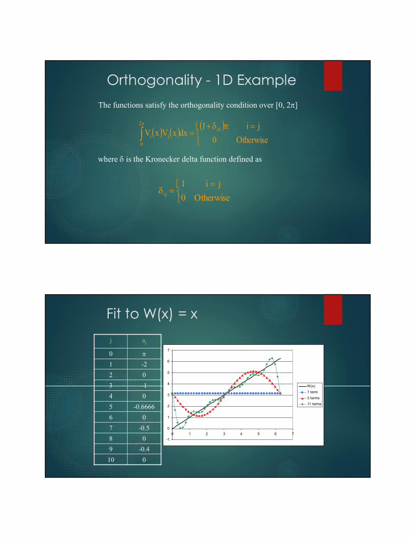
The functions satisfy the orthogonality condition over [0, 2]

Otherwise

ji

0

1dxxVxV 0i

2

0

ji

where is the Kronecker delta function defined as

Otherwise

ji

0

1ij

Fit to W(x) = x

j aj

0

1 -2

2 0

3 -1

4 0

5 -0.6666

6 0

7 -0.5

8 0

9 -0.4

10 0

-1

0

1

2

3

4

5

6

7

0 1 2 3 4 5 6 7

W(x)

1 term

3 terms

11 terms

Extension to Two Dimensions

In many cases, wavefronts take on a complex shape defined over a circular region and we wish to fit this surface to a series of simpler components.

Wavefront Fitting

=

-0.003 x

+ 0.002 x

+ 0.001 x

Unit Circle

x

y

r

q1

Divide the realradial coordinateby the maximum radiusto get a normalizedcoordinate r

Orthogonal Functions on the Unit Circle

Taylor polynomials (i.e. 1, x, y, x2, xy, y2,….) are not orthogonal on the unit circle.

qrrqrqr

Otherwise

ji

0

Cdd),(V),(V j

j

2

0

1

0

i

where Cj is a constant for a given j

Many solutions, but let’s try something with the form

qrqr iii R),(V

Orthogonal Functions on the Unit Circle

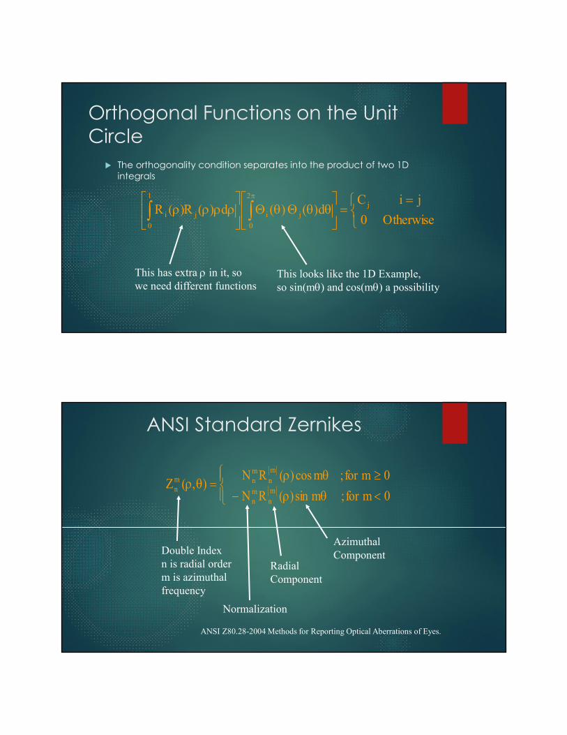
The orthogonality condition separates into the product of two 1D integrals

qqq

rrrr

Otherwise

ji

0

Cd)( )(d)(R)(R j

j

2

0

ij

1

0

i

This looks like the 1D Example,so sin(mq) and cos(mq) a possibility

This has extra r in it, so we need different functions

ANSI Standard Zernikes

qrqr

qr 0 mfor ; msin)(RN

0mfor ; mcos)(RN),(Z

mn

mn

mn

mnm

n

Double Indexn is radial orderm is azimuthal frequency

Normalization

RadialComponent

AzimuthalComponent

ANSI Z80.28-2004 Methods for Reporting Optical Aberrations of Eyes.


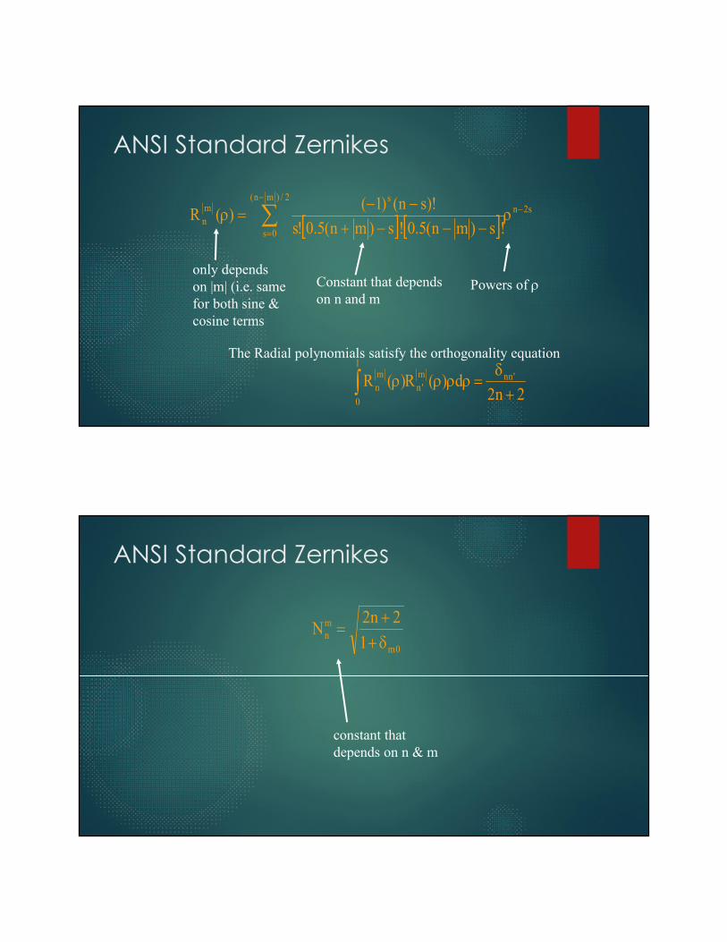
only dependson |m| (i.e. samefor both sine &cosine terms

Powers of r

s2n

2/)mn(

0s

smn ! s)mn(5.0! s)mn(5.0!s

)!sn()1()(R

r

r

Constant that dependson n and m

2n2d)(R)(R 'nnm

'n

1

0

mn

rrrr

The Radial polynomials satisfy the orthogonality equation


constant thatdepends on n & m

0m

mn 1

2n2N

Orthogonality

qrrqrqr

Otherwise

m'm;n'n for

0

Cdd),(Z),(Z mn,m

n

2

0

1

0

'm'n

rrrr

q

qq

qq

Otherwise

m'm;n'n for

0

Cd)(R)(R

dmsin

mcos

'msin

'mcosNN

mn,mn

1

0

'm'n

2

0

mn

'm'n

Orthogonality

Otherwise

m'm;n'n for

0

C

2n2 1NN mn,n'n

0mm'mmn

'm'n

This equals zerounless m=m’ This equals zero

unless n=n’So this portion issatisfied

What happens when n=n’ and m=m’?

Orthogonality

mn,0m

2mn C

2n2

1 1 N

When n=n’ and m=m’

m,n0mm0

C2n2

1 1

1

22n

m,nC

Orthogonality

m'mn'nmn

2

0

1

0

'm'n dd),(Z),(Z qrrqrqr

The First Few Zernike Polynomials

qrqr

rqr

qrqr

qrqr

qrqr

qr

26

123

26

2

2

1

222

202

222

11

11

00

cos,Z

,Z

sin,Z

cos,Z

sin,Z

,Z

Zernike Polynomials

Azimuthal Frequency, q

Rad

ialP

olyn

omia

l, r

Z00

Z11Z1

1

Z20

Z31 Z3

1

Z40 Z4

2

Z22

Z42

Z33 Z3

3

Z44Z4

4

Z22

Caveats to the Definition ofZernike Polynomials

At least six different schemes exist for the Zernike polynomials.

Some schemes only use a single index number instead of n and m. With the single number, there is no unique ordering or definition for the polynomials, so different orderings are used.

Some schemes set the normalization to unity for all polynomials.

Some schemes measure the polar angle in the clockwise direction from the y axis.

The expansion coefficients depend on pupil size, so the maximum radius used must be given.

Some groups fit OPD, other groups fit Wavefront Error.

Make sure which set is being given for a specific application.

Another Coordinate System

x

y

rf

Normalized Polar Coordinates:

f

r

y

xtan

r

r

1

max

1

r ranges from [0, 1]f ranges from [-180°, 180°]

NON-STANDARD

Zernike Polynomials - Single Index

Azimuthal Frequency, q

Rad

ialP

olyn

omia

l, r

Z0

Z1

Z4 Z5Z3

Z9Z8Z7Z6

Z10 Z11 Z12 Z13 Z14

Z2

ANSI/ISO STANDARD

Starts at 0Left-to-RightTop-to-Bottom

Other Single Index Schemes

Z1

Z3

Z4 Z6Z5

Z10Z8Z7 Z9

Z15Z13Z11 Z12 Z14

Z2

NON-STANDARDStarts at 1cosines are even termssines are odd terms

Noll, RJ. Zernike polynomials and atmospheric turbulence. J Opt Soc Am 66; 207-211 (1976).

Also Zemax “Standard Zernike Coefficients”


Z1

Z3

Z4 Z5 Z6

Z10Z7 Z8 Z11

Z18Z13Z9 Z12 Z17

Z2

NON-STANDARDStarts at 1increases along diagonalcosine terms first35 terms plus two extraspherical aberration terms.No Normalization!!!

Zemax “Zernike Fringe Coefficients”

Also, Air Force or University of Arizona


Born & Wolf

Malacara

Others??? Plus mixtures of non-normalized, coordinate systems.

NON-STANDARD

Use two indices n, m to unambiguously define polynomials.Use a single standard index if needed to avoid confusion.

Examples

Example 1:

4m

0.25 D of myopia for a 4 mm pupil (rmax = 2 mm)

qrqrr

r

,Z34000

1,Z

4000

1

20008000

2

8000

rW 0

200

222

4mm

Examples

Example 2:

1m

1.00 D of myopia for a 2 mm pupil (rmax = 1 mm)

qrqrr

,Z34000

1,Z

4000

1

20002000

rW 0

200

22

2mm

Same Zernike Expansion as Example 1, but different rmax.

Always need to give pupil size with Zernike coefficients!!

RMS Wavefront Error

RMS Wavefront Error is defined as

frr

frrfr

m all,1n

2m,n

2

WFE add

dd)),(W(RMS

Zeroth Order Zernike Polynomials

Z00

This term is called Piston and is usually ignored.The surface is constant over the entire circle, sono error or variance exists.

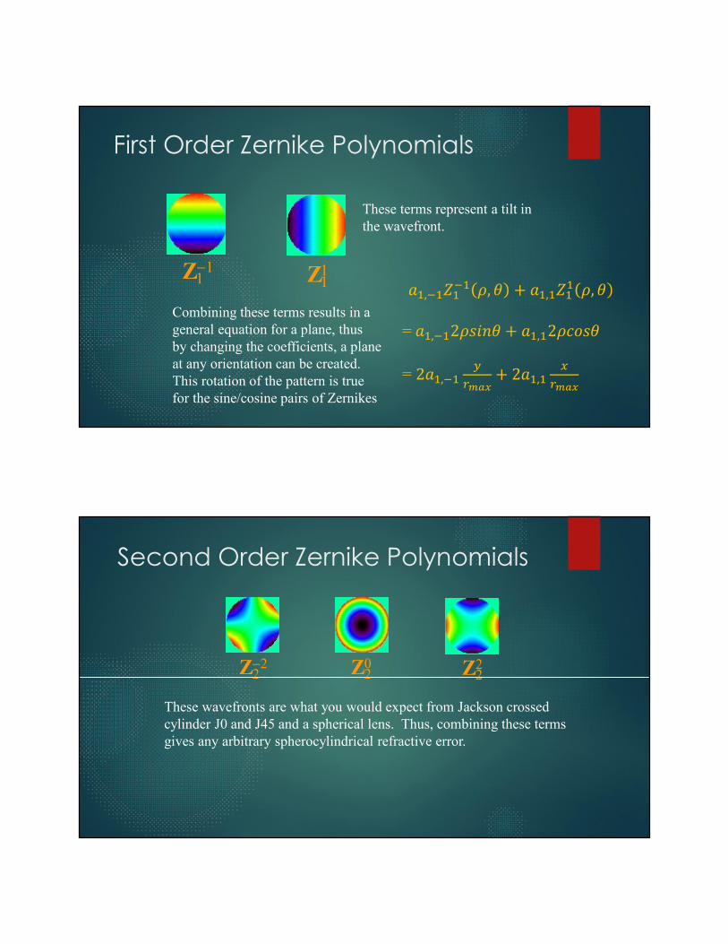
First Order Zernike Polynomials

Z11Z1

1

These terms represent a tilt in the wavefront.

Combining these terms results in ageneral equation for a plane, thusby changing the coefficients, a planeat any orientation can be created.This rotation of the pattern is truefor the sine/cosine pairs of Zernikes

𝑎 , 𝑍 𝜌, 𝜃 + 𝑎 , 𝑍 𝜌, 𝜃

= 𝑎 , 2𝜌𝑠𝑖𝑛𝜃 + 𝑎 , 2𝜌𝑐𝑜𝑠𝜃

= 2𝑎 , + 2𝑎 ,

Second Order Zernike Polynomials

Z20 Z2

2Z22

These wavefronts are what you would expect from Jackson crossedcylinder J0 and J45 and a spherical lens. Thus, combining these termsgives any arbitrary spherocylindrical refractive error.

Third Order Zernike Polynomials

Z31 Z3

1Z33 Z3

3

The inner two terms are coma and the outer two terms are trefoil. These terms represent asymmetric aberrations that cannot be corrected with convention spectacles or contact lenses.

Fourth Order Zernike Polynomials

Z40 Z4

2Z42 Z4

4Z44

SphericalAberration

4th orderAstigmatism

4th orderAstigmatismQuadroil Quadroil

These terms represent more complex shapes of the wavefront.Spherical aberration can be corrected by aspheric lenses.

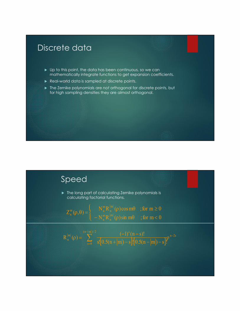
Discrete data

Up to this point, the data has been continuous, so we can mathematically integrate functions to get expansion coefficients.

Real-world data is sampled at discrete points.

The Zernike polynomials are not orthogonal for discrete points, but for high sampling densities they are almost orthogonal.

Speed The long part of calculating Zernike polynomials is

calculating factorial functions.

qrqr

qr 0 mfor ; msin)(RN

0mfor ; mcos)(RN),(Z

mn

mn

mn

mnm

n

s2n

2/)mn(

0s

smn ! s)mn(5.0! s)mn(5.0!s

)!sn()1()(R

r

r

Least Squares Fit

)y,x(f

)y,x(f

)y,x(f

a

a

a

a

)y,x(Z)y,x(Z)y,x(Z)y,x(Z



NN

22

11

nm

11

11

00

NNmnNN

11NN

11NN

00

22mn22

1122

1122

00

11mn11

1111

1111

00

FZZZA

FZZAZ

FZA

T1T

TT

Gram-Schmidt Orthogonalization

Examines set of discrete data and creates a series of functions which are orthogonal over the data set.

Orthogonality is used to calculate expansion coefficients.

These surfaces can then be converted to a standard set of surfaces such as Zernike polynomials.

Advantages

Numerically stable, especially for low sampling density.

Disadvantages

Can be slow for high-order fits

Orthogonal functions depend upon data set, so a new set needs to be calculated for every fit.

Shack-Hartmann Wavefront Sensor

Perfect wavefronts give a uniform grid of points, whereas aberratedwavefronts distort the grid pattern.

Least Squares Fit

FZZZA

FZZAZ

FZA

T1T

TT

Again, conceptually easy to understand, although this can be relatively slow for high order fits.

dy/)y,x(dW

dy/)y,x(dW

dy/)y,x(dW

dx/)y,x(dW

dx/)y,x(dW

dx/)y,x(dW

a

a

a

dy/)y,x(dVdy/)y,x(dVdy/)y,x(dV



dx/)y,x(dVdx/)y,x(dVdx/)y,x(dV



Z

NN

22

11

NN

22

11

J

2

1

NNJNN2NN1

22J222221

11J112111

NNJNN2NN1

22J222221

11J112111

Wavefront Reconstruction

PSF

class09 21 zernikes - wp.optics.arizona.edu

Documents