ISSN 1936-5071

Children’s Health Status in Uganda

Godfrey Bahiigwa Economic Policy Research Centre

Kampala, Uganda

and

Stephen D. Younger Cornell University Ithaca, New York

July, 2005

We are grateful to David Sahn and Peter Glick for comments. This research is supported SAGA, a cooperative agreement between USAID and Cornell and Clark-Atlanta Universities. See www.saga.cornell.edu.

2

Abstract This paper studies trends and determinants of children's standardized heights, a good overall measure of children's health status, in Uganda over the 1990s. During this period, Uganda made impressive strides in economic growth and poverty reduction (Appleton, 2001). However, there is concern that improvements in other dimensions of well-being, especially health, has been much weaker. We find that several policy variables are important determinants of children's heights. Most importantly, a broad package of basic health care services has a large statistically significant effect. Provision of some of these services, especially vaccinations, appears to have faltered in the late 1990s, which may help to explain the lackluster performance on stunting during that period. We also find that civil conflict, a persistent problem in some areas of the country, has an important (negative) impact on children's heights. Better educated mothers have taller children, but the only substantial impact is for children of mothers who have completed secondary school. Finally, we find that households that rely more on own-production sources of income tend to have more malnourished children, even after controlling for their overall level of income and a host of other factors. This latter conclusion is supportive of the Plan for Modernization of Agriculture, which aims to shift farmers from subsistence to commercial agriculture or other more productive activities. Keywords: height-for-age, Uganda JEL categories: I12, O55

1

1. Introduction Uganda has experienced rapid economic growth over the past fifteen years, with concomitant reductions in poverty (Appleton, 2001). This progress has been heralded as an impressive exception to African countries’ economic stagnation, and rightly so. But despite this progress, there is concern in Uganda that living standards are not improving by anything like the quantitative analysis of household expenditures suggests. Both of Uganda’s participatory poverty assessments find that focus group participants and key informants are only slightly more likely to say that poverty has declined rather than increased in their community (UPPAP, 2000, 2002). In addition, there is concern among policy makers and stakeholders that other dimensions of well-being, especially health, are not improving over time despite the substantial increases in Ugandans’ incomes (Ministry of Finance, Planning, and Economic Development, 2002; Task Force on Infant and Maternal Mortality, 2003; Uganda Bureau of Statistics, 2001; Ssewanyana and Younger, 2004). To date, most of this concern has centered around infant and child mortality rates, which improved rapidly as the country emerged from the protracted civil conflicts of the 1970s and 1980s, but then leveled off in the mid-1990s, even though economic growth continued. This paper pursues a similar concern, but regarding a separate indicator of well-being, children’s heights. The literature in nutritional sciences includes a wealth of studies showing that, in poor countries, children’s height is a particularly good summary measure of children’s general health status (Cole and Parkin 1977; Mosley and Chen, 1984; WHO, 1995). As summarized by Beaton et al (1990), growth failure is “…the best general proxy for constraints to human welfare of the poorest, including dietary inadequacy, infectious diseases and other environmental health risks.” They go on to point out that the usefulness of stature is that it captures the “…multiple dimensions of individual health and development and their socio-economic and environmental determinants (p. 2).” We believe that health is an important dimension of human well-being. In Sen’s terms, good health is a basic capability (Sen, 1979, 1985, 1987). In addition, children’s height is an interesting dimension of well-being to study because, surprisingly, it is not highly correlated with standard measures like income or expenditures per capita (Appleton and Song 1999; Haddad et al 2003).1 Studying the change in children’s health status, then, is a good complement to Appleton’s work on changes in economic measures of well-being in Uganda. In addition to presenting basic data on the evolution of children’s heights over time, to the extent that the data permit, we strive to be policy relevant by relating various indicators of policy to children’s heights. This includes some obvious variables such as information on the availability of a variety health care services, but some less obvious ones, such as the shares of household income coming from home production, commercial agriculture, and other off-farm sources. The latter is particularly relevant in the context of the Plan for Modernization of Agriculture (PMA), a major policy initiative that is an essential part of the country’s overall Poverty Eradication Action Plan (PEAP) (Ministry of Finance, Planning and Economic Development, 2004; Ministry of Finance, Planning and Economic Development, and Ministry of Agriculture, Animal Industry and Fisheries, 2000). 1 Pradhan, Sahn, and Younger (2003) give a more thorough defense of using children’s height as a welfare measure.

2

2. Data The data for this study come from two standard household surveys, the Demographic and Health Surveys (DHS), and the Uganda National Household Survey (NHS). The three DHS surveys, carried out in 1988, 1995, and 2000, are especially useful because they span a relatively long time period. Further, the three surveys are very closely comparable, having similar questionnaires. This allows us to pool the three data sets, yielding a large sample with which to investigate the correlations between policy and children’s health. There are, however, two important limitations to the DHS. First, due to a variety of localized civil conflicts, the sample frames are not identical for all three surveys. The first survey, in particular, did not sample about 20 percent of the population in the north and, to a lesser extent, west of the country. In order to combine all three surveys, we use only data for children residing in areas included in all three DHS surveys.2 The second limitation of the DHS data is that they do not include an income or expenditure variable. Nevertheless, Montgomery, et al. (2000), Filmer and Pritchett (2001), Sahn and Stifel (2003), and Stifel and Sahn (2000) have all shown that it is possible to construct a welfare variable from DHS data whose statistical properties are comparable to the standard household expenditure variable. All of these authors use either principal components or factor analysis to generate an index of household assets — including durable consumer goods, productive assets, and household education levels. In this paper, we use factor analysis to create an index based on consumer durables that the household owns and the household head’s years of education (Sahn and Stifel, 2000). Appendix 1 gives details of the index and its estimation. Finally, the DHS data do not include variables on agricultural activity that would allow us to relate the PMA to children’s health status. To address these issues, we use the 1999 NHS data. While the sample size is smaller, this survey includes a rich set of data on household’s agricultural activities, and on other income-earning activities. For both surveys, the sample comprises children under the age of 60 months (five years). For the DHS, these are the children of one woman age 15-49 selected randomly from each household in the sample. For the NHS, the sample is all children in the sample households. The dependent variable of interest in all of the analyses is children’s height, standardized by age and gender, and compared to a population of healthy children. This is done through the use of a height-for-age (and gender) z-score, defined as:

z-scoreix

mediani xxσ

−= ,

where xi is a child’s height, xmedian is the median height of children in a healthy and well-nourished reference population of the same age and gender, and σx is the standard deviation from the mean of the reference population.3 Thus, the z-score measures the number of standard

2 In practice, this seems to matter very little. All of our key results remain if we use the entire samples. 3 Following the recommendation of the WHO and the United States Centers for Disease Control, the reference sample of healthy children comes from the NHANES-III dataset in the United States.

3

deviations that a child’s height is above or below the median for a reference population of healthy children of her/his age and gender. We will describe the remaining variables in section 4 below.

3. Children’s Height over Time in Uganda – Cause for Concern Table 1 gives basic descriptive statistics for the height-for-age z-scores in the three Uganda DHS surveys. As with infant mortality rates (Ssewanyana and Younger, 2004), we see a marked improvement between 1988 and 1995, a result that is not too surprising given that Uganda was recovering from a civil war in this period, and then a modest and statistically insignificant deterioration between 1995 and 2000.

Table 1 - Height-for-age z-scores in Uganda, by DHS survey

survey mean median standard

deviation N1988 -1.79 -1.83 1.52 37021995 -1.58 -1.59 1.48 45192000 -1.62 -1.63 1.42 5145

It is possible to create a more detailed time series of children’s heights with the DHS data. Because each survey collects anthropometric data for children up to five years old, the DHS data provide heights and weights for children born in the five years immediately prior to the survey. So it is possible to find average z-scores for annual birth cohorts. There is, however, an important bias in this calculation. In malnourished populations, standardized heights tend to decline with age for children up to two or three years of age (Martorell and Habicht, 1986). Because the children born farther from the survey are older, their cohort will tend to be shorter relative to a healthy population than the younger cohorts born near the survey date. To correct this, we regress height-for-age z-scores on a quartic function of age plus a constant, and then consider the residual of that regression as an “age-adjusted height-for-age z-score.”

Figure 1 gives the results of this calculation. The diamonds are the simple annual averages; the solid line is a nonparametric regression of the age-adjusted height-for-age z-score on the year of birth;4 and the dotted lines show two standard deviations above and below the regression curve. Both the simple averages and the regression line show clear improvements in children’s health status beginning in the late 1980s through the mid-1990s. This was also a time of rapidly rising incomes. The averages are more difficult to interpret in the late 1990s because they vary significantly from year to year. The regression line, though, shows a clear reversal of the improving HAZs beginning in 1997. By 2000, the regression line is (just) outside the lower bound of the confidence interval for 1997, despite the fact that incomes continued to rise during

4 This regression uses a LOESS smoother with the bandwidth set at seven years, three years before and three after each year. At the extremes, we continue to include seven years in the bandwidth, with extra years after or before the given year as it approaches the beginning or end of the sample. Note that we included the years 1983, 1989, and 2001 in the estimation, but do not report them here as they have very few observations. 1990 has no observations.

4

this period. Clearly, something important changed with respect to children’s health in the late 1990s. We now turn to multiple regressions to try to understand the determinants of children’s heights and, inter alia, the reasons for this puzzling decline.

Figure 1 – Average height-for-age z-scores by birth cohorts in Uganda

-1.9

-1.85

-1.8

-1.75

-1.7

-1.65

-1.6

-1.55

-1.5

-1.45

1982 1984 1986 1988 1990 1992 1994 1996 1998 2000 2002

Year

Age

-adj

uste

d H

AZ

4. Determinants of Children’s Heights

4.1. Health Care, Household, Child, and Mother’s Characteristics We first consider the effect of a variety of household, child, and mother’s characteristics on children’s standardized height, using the combined DHS samples of children under five years old born to mothers age 15-44 at the time of birth. The strategy is a simple reduced form OLS regression. A brief description of the data follows. The sample is a combination of the first three rounds of DHS surveys in Uganda, with the following restrictions. First, while the full DHS sample includes women age 15-49, we eliminate women who were older than 44 at the time of their child’s birth to avoid a potential bias from sample truncation. Because we are lagging off the sampling date by up to five years, mothers of children who are older at the time of the survey could not have been older than 49 less the child’s age at the time of the survey. Since mother’s age is correlated with children’s nutritional status, a truncation bias could result, since the older children in the sample would have systematically younger mothers. To correct for this, we include only mothers between 15 and 44 at the child’s date of birth, which reduces the sample of children by less than one percent. A second limitation

5

on the sample is that not all districts in Uganda were sampled in each round of the DHS because of the civil conflict at the time of the surveys. We limit our analysis to only those areas that were sampled in all three DHS rounds, which reduces the sample of children by 11 percent. Because this is a large share of the sample, we have checked that none of our key results are sensitive to this limitation. For the household, we consider whether the household resides in an urban or rural area and the region of residence, with Central region, home of the capital city, being the left-out category. We also include the log of the household’s asset index, described in Appendix 1. Finally, we include information on the household’s main source of drinking water and toilet facilities. For water, the left-out category is a surface source (lake, stream, etc). For toilet facilities, it is no toilet. For the children, we include gender, age, and whether the child is a twin, triplet, etc. All of these factors are known to influence children’s height (Martorell and Habicht, 1986; Wilson, 1986). For the mothers, we include educational attainment, which can affect children’s heights directly through the mother’s ability to obtain and process health information, and indirectly through the mother’s ability to earn income, although to some extent, the asset index should also capture the latter. We also include the mother’s age and, in some regressions, height. These are also known to influence children’s heights. Unfortunately, mother’s height is not available for the 1988 data, so its inclusion limits the sample size and the time frame over which we have estimates. Thus, we do not include it in all regressions. Finally, we consider the mother’s marital status, a variable that may reflect the extent to which resources, both time and money, are available to her and her children. The last set of variables regards the availability of health care services. These are district-5 or cluster-level averages of individual responses to a variety of questions about the use of such services as vaccinations for children up to the age of two; mother’s knowledge of oral rehydration therapy; prenatal and birthing care by any medical professional and, in particular, a doctor; and use of modern contraceptive methods. We use these averages rather than the individual mother’s or child’s response to avoid the possible endogeneity of individual-level data on service use. Table 2 gives the mean for each regressor and its standard error. Table 2 - Descriptive statistics, DHS data 1988 1995 2000

Variable mean s.e. mean s.e. mean s.e.Region/area

Central 0.296 0.055 0.319 0.050 0.311 0.052Eastern 0.284 0.064 0.256 0.048 0.266 0.050

Northern 0.057 0.033 0.124 0.041 0.125 0.041Western 0.363 0.068 0.301 0.050 0.299 0.049

5 The district-level averages are for the year in which the child was born. The cluster-level averages are for the year of the survey.

6

Rural 0.914 0.018 0.876 0.024 0.896 0.019ln(HH asset index) 0.293 0.016 0.361 0.017 0.411 0.017Water supply

Surface source 0.341 0.032 0.263 0.027 0.141 0.019Piped water 0.024 0.006 0.017 0.004 0.010 0.002

Public tap 0.041 0.010 0.054 0.011 0.070 0.013Well water 0.498 0.035 0.654 0.026 0.730 0.021

Toilet facility Flush toilet 0.027 0.008 0.013 0.004 0.011 0.003

Latrine 0.802 0.024 0.846 0.017 0.824 0.018Other toilet 0.009 0.003 0.006 0.002 0.044 0.005

No toilet 0.162 0.024 0.135 0.017 0.121 0.016Child characteristics

Female 0.508 0.007 0.510 0.011 0.503 0.009Multiple birth 0.026 0.003 0.027 0.004 0.021 0.003

Age 26.933 0.253 21.578 0.182 27.865 0.247Mother’s education

Incomplete primary 0.328 0.013 0.400 0.013 0.426 0.012Complete primary 0.179 0.013 0.199 0.012 0.223 0.012

Incomplete secondary 0.051 0.007 0.081 0.007 0.080 0.008Complete Secondary 0.030 0.006 0.043 0.005 0.039 0.005

Mother’s age at birth 26.420 0.207 25.807 0.170 26.106 0.138Mother’s height n.a. n.a. 157.252 0.252 157.515 0.291Mother’s marital status

Never married 0.036 0.004 0.029 0.004 0.029 0.005Married 0.864 0.011 0.889 0.009 0.888 0.008

Separated 0.100 0.010 0.082 0.007 0.083 0.006Polygynous union 0.278 0.016 0.247 0.013 0.229 0.012

Health care indicators Received any vaccination /1 0.700 0.011 0.811 0.009 0.873 0.009Received all vaccinations /1 0.387 0.017 0.398 0.014 0.365 0.012

Knowledge of ORT /2 0.457 0.026 0.749 0.017 0.922 0.008Use of modern contraception /2 0.039 0.005 0.113 0.011 0.202 0.013

At least one tetanus toxoid /1 0.565 0.019 0.799 0.008 0.733 0.009Prenatal care by professional /1 0.871 0.015 0.858 0.007 0.870 0.013

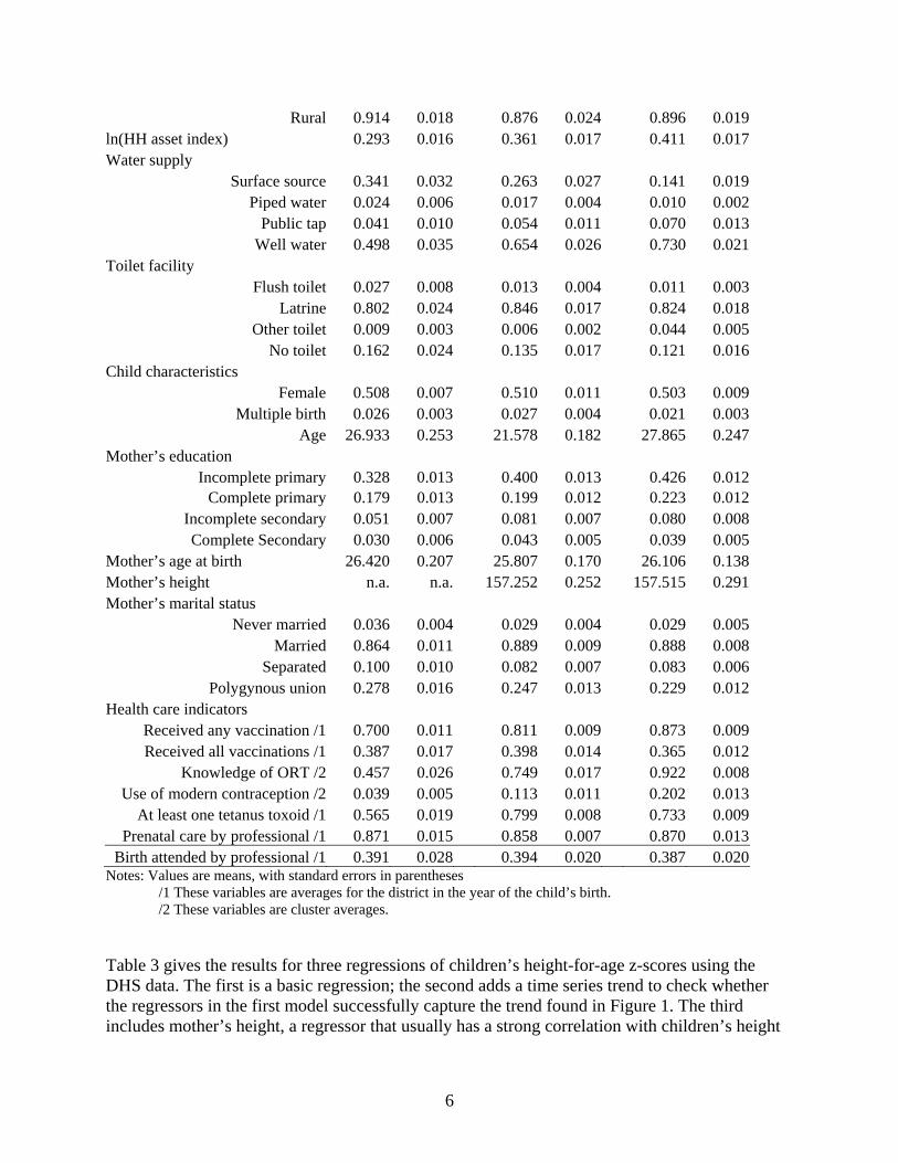
Birth attended by professional /1 0.391 0.028 0.394 0.020 0.387 0.020Notes: Values are means, with standard errors in parentheses /1 These variables are averages for the district in the year of the child’s birth. /2 These variables are cluster averages. Table 3 gives the results for three regressions of children’s height-for-age z-scores using the DHS data. The first is a basic regression; the second adds a time series trend to check whether the regressors in the first model successfully capture the trend found in Figure 1. The third includes mother’s height, a regressor that usually has a strong correlation with children’s height

7

for both genetic and phenotypic reasons, but which limits the sample to the last two rounds of the DHS data. Controlling for other variables, children in Western region, generally regarded as less poor than either Eastern or Northern, are nevertheless significantly shorter than children in Eastern and Northern region, though not Central region, an anomalous result that has been noted elsewhere (Uganda Bureau of Statistics, 2001). Children living in rural areas are not significantly shorter than those in urban areas, again, holding all else constant.

Table 3 - Regression results for children’s HAZ in Uganda

Basic model with trend with mother’s height Regressor beta t beta t beta t

Region/area Eastern 0.071 1.25 0.085 1.51 0.161 2.58

Northern 0.102 1.01 0.115 1.15 0.085 0.86Western -0.074 -1.07 -0.076 -1.11 0.086 1.15

Rural -0.061 -0.90 -0.043 -0.60 -0.079 -1.24ln(HH asset index) 0.536 9.43 0.540 9.42 0.530 8.55Water supply

Piped water 0.216 1.82 0.218 1.83 0.095 0.63Public tap -0.018 -0.22 -0.011 -0.13 -0.089 -1.06

Well water 0.079 1.83 0.077 1.78 0.011 0.19Toilet facility

Flush toilet -0.003 -0.03 -0.004 -0.04 -0.089 -0.53Latrine 0.025 0.48 0.021 0.41 -0.003 -0.06

Other toilet 0.349 1.47 0.348 1.47 0.181 0.73Child characteristics

Female 0.150 5.63 0.150 5.60 0.125 4.00Multiple birth -0.629 -5.28 -0.628 -5.30 -0.561 -4.05

Age -0.210 -13.23 -0.211 -13.27 -0.206 -10.10Age^2 0.008 7.59 0.008 7.60 0.008 5.64Age^3 -1.35E-04 -4.64 -1.36E-04 -4.66 -1.31E-04 -3.45Age^4 7.50E-07 2.96 7.60E-07 3.00 7.19E-07 2.22

Mother’s education Incomplete primary -0.007 -0.17 -0.007 -0.17 -0.010 -0.19

Complete primary 0.084 1.79 0.083 1.76 0.125 2.31Incomplete secondary 0.076 1.21 0.074 1.17 0.081 0.97Complete Secondary 0.218 2.60 0.211 2.53 0.254 2.85

Mother’s age at birth 0.017 6.45 0.017 6.56 0.014 4.07Mother’s height 0.020 4.010Mother’s marital status

Never married 0.005 0.07 0.003 0.04 0.092 0.64Separated -0.017 -0.29 -0.019 -0.33 -0.007 -0.09

Polygynous union -0.078 -2.09 -0.079 -2.14 -0.106 -2.42

8

Health care indicators Any vaccination received /1 -0.116 -0.82 -0.036 -0.24 -0.155 -0.81All vaccinations received /1 -0.161 -1.39 -0.208 -1.80 -0.203 -1.24

Tetanus toxoid in pregnancy /1 0.028 0.23 -0.166 -1.17 -0.003 -0.02Any professional prenatal care /1 0.107 0.44 0.174 0.69 0.532 2.07

Any professional birth attendant /1 0.427 3.16 0.398 2.79 0.539 3.83Use of modern birth control /2 0.335 1.83 0.420 2.15 0.527 2.82

Mother knows of ORT /2 0.072 0.68 0.134 0.91 -0.297 -1.82Trend 0.181 2.12 Trend squared -0.002 -2.20 Constant -1.032 -4.14 -4.782 -2.60 -4.107 -5.43 Household assets have a strongly significant correlation with children’s heights. While this might seem obvious — richer households should have healthier children, other things equal — it is common to find only a weak correlation (Appleton and Song 1999; Haddad et al., 2003). The coefficient suggests that a doubling of the asset index yields an increase of about 0.54 z-scores. Note that even though the asset index is not measured in monetary units, its 40 percent increase between 1988 and 2000 is quite similar to the 44 percent increase in GDP per capita over the same period. This 40 percent increase yielded an improvement of 0.24 z-scores. The water supply variables are jointly significant (F3,485 = 2.50), but only indoor taps and wells (at the 10 percent level) are individually significant. (Surface water plus “other water” is the base category.) These effects are rather modest, about 0.22 z-scores for piped water, which only very few households have in Uganda, and 0.08 z-scores for well water. Furthermore, note that in Model 3, this effect disappears (F4,363 = 1.20 for all the water variables). We have checked that this is a function of the sample for this model, which excludes the 1988 data, not the inclusion of mother’s height. Thus, the significant water impact in Models 1 and 2 is driven only by the 1988 data. Note, too, that the “other water” source is significantly larger in 1988 (Table 2) which may suggest that some sources were classified differently in that survey. Overall, we have to conclude that there is only modest evidence of a link between the household’s principal water source and children’s health. The same is true for the type of toilet. These variables are jointly insignificant in all three models. While the “other” category has a large coefficient, this accounts for a very small percentage of the toilet facilities in Uganda (Table 2). Such results are certainly counterintuitive, though they are not atypical for this sort of regression. Strauss and Thomas’s (1995) review of the literature on health production functions notes that it is not uncommon to find that household water supply and toilet facility are not correlated with children’s health variables. One possible explanation for such anomalous results is that these variables do not measure well what we expect them to measure. In particular, what makes children sick, and therefore causes them to grow more slowly, are pathogens in their environment. We assume that water from protected wells is less likely to be contaminated with such pathogens than is surface water, and that households with access to a latrine or flush toilet are also less likely to be exposed to pathogens, but that may be less so than we assume. Wells can be contaminated, for example, or people whose main source is a well may also use surface

9

water at times. Similarly, latrines can be poorly constructed or maintained. In such cases, the advantages of these water and sanitation services may be less than we suppose. Other things equal, girls are significantly taller than boys relative to the reference standards (which control for gender). Children of multiple births are far shorter than those from single births. And children are significantly more likely to be short relative to the reference standards as they grow older. All of these results are consistent with the literature on child growth in poor countries. Note that because age is included as a fourth-order polynomial, interpretation of its coefficients is not obvious. Figure 2 maps the predicted relationship based on the first model in Table 3, along with a non-parametric regression of height-for-age on age. The polynomial approximation is clearly quite good. Predicted standardized heights decline dramatically -- almost two z-scores -- with age up to about 20 months, at which point they level off. As with children in other poor health environments, the cumulative impact of disease and poor feeding causes Ugandan children to fall behind the reference group of healthy children more or less continuously up to age two, and there is no sign of “catch-up” growth at older ages (Martorell and Habicht, 1986).

Figure 2 - Predicted HAZ by Age in Uganda

-2.5

-2

-1.5

-1

-0.5

0

0 10 20 30 40 50 60

Age (months)

Hei

ght-

for-

age

z-sc

ore

LoessModel 1

Except for mothers that did not complete primary school, mother’s education has a significant relationship with children’s heights. This steps up once for primary graduates, whose children are about 0.08 z-scores taller than children of mothers with no education, and again for secondary graduates, whose children are 0.21 z-scores taller. These results are also rather modest in absolute terms, especially since Uganda’s greatest success in education has been the enrolment of more girls in primary school, while graduation rates have been disappointing. But as the regression results make clear, simply enrolling girls has no benefits for their children’s heights

10

when they become mothers. Girls must successfully graduate primary school to have even a small impact, while the larger gains are for the children of secondary school graduates, who remain quite rare in Uganda (Table 2). Mother’s age also has a significant relationship with children’s height, though it is very small. Children of taller mothers also tend to be relatively taller. For each centimeter of mother’s height, the child’s z-score averages 0.02 higher. The interquartile range for mother’s height is 8.1 centimeters, so moving from the 25th to the 75th percentile increases a child’s height by 0.16 z-scores on average, also a modest gain. Mother’s marital status has interesting impacts on children’s heights. Compared to married mothers, those that were never married and/or separated from their husband (by divorce or death) have children who are about the same height, which is surprising. Children of mothers in polygynous households, however, are significantly shorter by about 0.08 z-scores, than children of never-married mothers. The results for some of the health care variables are often counter-intuitive. Most have individually insignificant t-statistics, but an F-statistic for their joint significance does reject the null hypothesis that these variables are unrelated to children’s heights. More puzzling, the vaccinations variables have the “wrong” sign. We believe that it is inappropriate to conclude that these services have a negative effect on children’s heights. Rather, the high correlation between the health care regressors is confounding the estimates. It tends to be the case that districts with high rates of vaccination also have high knowledge of oral rehydration, high rates of tetanus toxoid injections during pregnancy, high rates of professional birth attendance, etc. This, combined with the fact that there is relatively little variation in these variables because they are district-level averages, leads to multicollinearity problems. Thus, while it would be interesting and useful to policy makers to be able to distinguish between the effects of tetanus toxoid injections vs. professional birthing assistance, etc., these data do not allow such fine analysis. Rather, we think that the best that we can do is sum up all of the health-care indicators, concluding that children in districts that have 100 percent vaccination rates, tetanus toxoid injections, professional prenatal and birthing care, knowledge of oral rehydration therapy, and modern methods of birth control would have children with z-scores that are, on average, 0.69 to 0.94 z-scores higher than children in districts with none of these services. These are by far the largest impacts that we find in this model, indicating that availability of basic health care is critical for lowering stunting rates in Uganda.

4.1.1. Impact on Stunting Rates Regression coefficients such as those in Table 3 show the impact of the regressor on the expected value, or mean, of the dependent variable, other things equal. While this information is useful, policy makers’ concern with children’s height is usually focused on the lower end of the distribution, not the mean, i.e, they are concerned with stunting rates, typically defined as the share of the population below -2 height-for-age z-scores. Table 4 gives the actual rate of stunting for each of the DHS surveys along with predicted rates from various policy simulations. These simulations shift the mean expenditure by the amount predicted in the basic model of Table 3

11

and then recalculate the share of the sample below -2 z-scores. Thus, the assumption is that the distribution of heights shifts right while maintaining its observed dispersion. This is consistent with much of the research on improvements in height-for-age in populations (WHO, 1995). With an eye toward the Millennium Development Goals, which are targeted for 2015, we simulate policy changes that seem feasible for that year. While there is no specific Millennium Development Goal for children’s stature, there is one to reduce “hunger” by half. We might interpret this goal as aiming to reduce stunting, though it is clearly more general than that.

Table 4 - Actual and simulated stunting rates

Stunting rate ImprovementBase rate in sample 0.41

Simulation Increase in assets 0.34 16%

100% primary graduates 0.39 4%Increase secondary graduates 0.40 3%

100% increase in secondary grads 0.35 14%100% basic health care 0.35 13%

Water supply improvement 0.40 3%

All of the above improvements/1 0.26 36%/1Includes all changes except the 100% increase in secondary school graduation. The first simulation assumes that household assets continue to accumulate until 2015 at the same average annual rate observed between 1988 and 2000. This has a significant impact on stunting, reducing it by 16 percent. Nevertheless, at just over one percent per year, it would take almost 100 years for asset accumulation alone to eliminate stunting in Uganda. The second simulation assumes that all mothers have at least a complete primary education. Given the success of Uganda’s Universal Primary Enrolment program, this seems a plausible simulation (Murphy, Bertoncino, and Wang, 2002). Nevertheless, its impact on stunting is rather small, only a four percent improvement. The third simulation assumes that by 2015, the rate of secondary school graduation among mothers is the same as today’s primary graduation rate (about 22 percent). This too, has only a limited impact on stunting. Increasing secondary graduation rates to 100 percent, which clearly is overly optimistic for 2015, would have a much larger impact. The fifth simulation assumes that all Ugandans have access to and use a basic health care package that includes professional prenatal care and birthing assistance, all recommended vaccinations, tetanus toxoid injections for pregnant women, and knowledge of oral reyhdration therapy.6 This has a large effect on stunting, reducing it by 13 percent. 6 Note that we have not altered the usage rates for modern contraception, since 100 percent usage is not a desirable policy outcome. However, the large coefficient on this variable in Table 3 suggests that if usage rates were to increase from their present 20 percent, stunting would fall significantly.

12

The sixth simulation assumes that all urban Ugandans have piped water in their homes, while all rural Ugandans have access to a well. This has only a small impact on stunting rates. Finally, combining all of these simulations, stunting would fall by 36 percent to 0.26, a substantial improvement, but still short of the presumed goal of halving stunting by 2015. The second regression in Table 3 adds a quadratic time trend to the model. Our interest here is to see whether the variables in the basic model adequately capture the trends in children’s heights, or whether there are important unexplained factors that have caused them to change consistently in one direction over time. The trend variables are not significantly different from zero, so there no evidence that an unexplained trend in children’s heights will help to improve the situation of child health Uganda.

4.2. Agricultural Modernization and Children’s Health In addition to the effects of standard health policy, there is concern in Uganda about how the Plan for Modernization of Agriculture (PMA) might affect children’s health status. The PMA is a broad, multifaceted program (Ministry of Finance, Planning and Development, and Ministry of Agriculture, Animal Industry, and Fisheries, 2000). Not all of its policy goals are easily analyzed with household survey data, but a key feature of the transformation of agriculture is that households should move out of subsistence farming into more commercial activities, on and off the farm, and into wage labor activities, possibly in the agricultural sector. In this section, we examine whether and how such changes might affect children’s nutritional status. In particular, we address the concern that as households shift out of food crop production for their own consumption, children’s nutritional status will suffer. Von Braun and Kennedy (1994) study this question for a number of countries, usually finding that this is not the case. However, no one has asked this question for Uganda, a gap that we now attempt to fill. Because our interest is the impact of agricultural transformation on children’s health status, we must change data sets to one that includes information on household incomes, the 1999 NHS. This survey also includes a variety of child, household, and community level data that are useful for modeling children’s heights. Columns 1 and 2 of Table 5 give means and their standard errors for the data used. Note that these data and the regressions that follow are for rural households only, because our focus is on the PMA.

13

Table 5 - Height-for-age z-score regressions from the 1999 NHS

OLS 2SLS mean s.d. coeff t-stat coeff t-stat ln(HH expenditures p.c.) 8.474 0.532 0.176 3.66 0.052 0.63Household income shares

Own production 0.258 0.161 -0.331 -2.52 -0.901 -1.30Commercial production 0.384 0.198 -0.091 -0.86 -0.227 -0.43

Formal sector wages 0.022 0.103 0.162 0.77 1.942 1.21Informal sector wages 0.066 0.154 -0.118 -0.78 -1.047 -1.11

HH Enterprise 0.102 0.180 0.096 0.71 1.610 1.61Other income 0.168 0.152 0.282 1.82 -1.377 1.28

Child Characteristics

Age (in months) 29.961 16.324 -0.180 -5.60 -0.189 -5.31Age^2 0.006 2.81 0.007 2.93Age^3 0.000 -1.36 0.000 -1.70Age^4 0.000 0.52 0.000 0.98

Female 0.502 0.500 0.186 3.83 0.163 3.04Region

Eastern 0.334 0.472 -0.106 -1.03 -0.158 -1.46Western 0.274 0.446 -0.135 -1.03 -0.106 -0.81

Northern 0.184 0.388 0.214 1.41 0.078 0.48Parent’s Characteristics

Mother literate 0.510 0.500 -0.063 -0.90 -0.127 -1.46Mother’s years of school 3.660 3.386 -0.002 -0.18 -0.005 -0.35Father’s years of school 5.778 3.722 0.012 1.53 0.000 0.04

Household size 7.310 3.404 0.021 2.56 0.017 1.66Civil unrest

1990/1991 0.030 0.170 0.288 1.18 0.204 0.691992/1993 0.032 0.177 0.040 0.15 0.226 0.831994/1995 0.026 0.160 -0.248 -1.03 -0.277 -1.101996/1997 0.052 0.222 -0.365 -2.35 -0.310 -1.831998/1999 0.054 0.225 -0.054 -0.29 0.008 0.04

ln(distance to health center) 1.645 0.804 -0.064 -1.82 -0.034 -0.87ln(distance to Kampala) 5.388 0.743 -0.057 -0.73 -0.055 -0.68ln(distance to district capital) 3.403 0.863 -0.014 -0.37 -0.019 -0.46ln(distance to municipality) 3.859 1.026 -0.002 -0.07 -0.026 -0.75Health center characteristics

Hours open per week 129.151 54.938 0.000 0.50 0.000 0.38Malaria drugs available 0.990 0.098 0.152 0.75 0.243 1.31

Antibiotics available 0.943 0.228 0.150 1.37 0.187 1.60Oral rehydration available 0.962 0.190 0.150 1.13 0.223 1.87

Immunizations available 0.819 0.382 -0.098 -1.25 -0.097 -1.15ln(average health center fee) 5.450 2.058 0.010 0.71 0.016 0.95

14

ln(average malaria drug cost) 4.741 3.022 0.043 1.30 0.049 1.26ln(average antibiotic cost) 4.700 3.050 -0.019 -0.60 -0.021 -0.57

Constant -1.346 -2.27 0.057 0.06 R-square 0.091 Tests for multiple coefficients F alpha F alpha

Income share variables 1.97 0.07 2.03 0.07Income shares except own prod 0.48 0.75 2.16 0.07

Civil strife variables 2.38 0.04 1.84 0.10Health center characteristics 2.00 0.08 3.41 0.00

Health center fees 2.64 0.05 2.94 0.03 Household expenditure is a broad measure of the households consumption (Uganda Bureau of Statistics, 2003).7 Household income shares are divided into six income sources: home production of agricultural goods, agricultural sales, formal sector employment earnings,8 informal sector employment earnings, profits from household enterprises, and other income. The latter is composed of imputed rents to owner occupied housing (31%), other rent and capital income (2%), remittances (24%), and inheritances, alimony, scholarships, pensions, and family allowances (43%). It is reasonable to ask why we should expect the source of household income to influence children’s health after controlling for the overall level of income (through the per capita expenditures variable). The literature includes two main concerns.9 First, income from home production is not fungible in the same way that other, cash, income is. As a result, a high proportion of home-produced income may shift consumption patterns toward more food which, in turn, may improve children’s nutritional status. Shifting toward more cash income, in turn, may shift consumption toward other things that, while increasing adults’ utility, may harm children’s growth prospects. Figure 3 provides a simple example in which there are two consumption goods, food and non-food. Assume that the household has two income sources, one exogenous source of cash and one from own-production/consumption of food. Also assume that the household can purchase food, but not sell it, and that nonfood items can be purchased, but not produced. In these circumstances, the budget constraint is kinked, turning vertical at the point where non-food consumption is equal to cash income. If the indifference curve is tangent to the budget constraint at this kink, then the household uses all of its cash income to buy nonfood items, and it consumes exactly the food that it produces, with no further purchases of food. In such a case, an increase in the share of home production in income will force an increase in the share of food in total consumption. This, in turn, may improve children’s nutritional status.

7 We are grateful to Simon Appleton for providing us with the expenditure aggregate. 8 Formal sector employment is defined as those employed in their main job as an employer, public employee, or political, social, or religious worker. 9 The volume edited by von Braun and Kennedy is the most comprehensive treatment, although it usually does not find that the empirical evidence supports these concerns.

15

Figure 3 - Optimal consumption of food and non-food with rationing

non-food consumption

food

con

sum

ptio

n

The second concern is that a shift toward greater cash income may shift control of resources away from women and toward men. This is because in some cultures, including in Uganda, men have more control over the marketing of agricultural production, while women have more control over home production (UPPAP, 2002). If women place a higher value on children’s health than men do, then shifting household income from home production to commercial sales may also reduce children’s health status. The child and parent characteristics are defined as in the DHS data and are self-explanatory. The civil unrest variables are one if a community leader reported that there had been civil unrest, military conflict, or large-scale conscription in the time period indicated, and zero otherwise. Our interest here is to examine the possible costs in terms of child health of the periodic local conflicts that have plagued Uganda over the past decade, especially in the North. The distance variables are self-explanatory. Our main interest is to identify the effect of distance to health care (the first variable) on children’s well-being. However, we also include the other distance variables to control for the fact that distance to a health center might proxy for a variety of other factors associated with remoteness. The health care characteristics are for the nearest public health center. The availability of various medicines is recorded as a dummy variable, while the log of the costs of fees and charges for malaria drugs and antibiotics are recorded in shillings.

16

Table 5 presents regressions of height-for-age z-scores on child, household, and community characteristics. Columns 3 and 4 report an ordinary least squares regression. However, the income share variables may well be jointly determined with children’s heights and so endogenous to this model. For example, households with unobserved characteristics such as a strong desire for healthy children may make occupational choices that are influenced by the value that they place on child health. If working closer to home permits greater attention to children, we may find that agricultural production or informal employment are positively correlated with children’s health, but the relationship is not causal. Own production may not cause children to be healthier, but simply reflect the parents’ underlying concern for child health. For that reason, the coefficients on income shares may be biased. To correct for such biases, we use two-stage least squares, reported in columns 5 and 6 of Table 5. The instrument list includes the log of the value of household durable goods, land holdings, business assets, and livestock holdings; the logs of wages for men and women in the community, for agricultural and non-agricultural employment; the log of prices of agricultural inputs (hoes, plows, pangas, wheelbarrows, diesel fuel, engine oil, bulk fertilizer, and retail fertilizer) and of cotton and coffee prices; the ratio of harvest-to-planting season prices and the ratio of farmgate to market prices in the harvest season for each of the crops recorded in the survey. The coefficients on income shares are constrained to sum to zero, so the estimated effect of an increase in any individual share must be equal and opposite to the sum of the effects of the other shares. The coefficient on own production is negative and significantly different from zero in the OLS regression. It is negative, much larger, but statistically insignificant in the 2SLS regression. These results run counter to the intuition discussed above: own production reduces children’s heights, other things (including total expenditures) equal. By implication, larger shares of other other income sources increase children’s heights. None of the other share coefficients are significantly different from zero individually, nor is any combination of four of the five remaining shares significant. Thus, we cannot say which income sources have a positive effect on children’s health, but we do know that at least one must, and that own production has a negative effect. Taken at face value, this is good news for the PMA, which aims to move farmers from home production to greater market sales. At a minimum, there is no evidence that, for a given overall expenditure level, shifts out of own production into commercial or wage activities worsens children’s nutritional status. The OLS regression suggests the opposite, while the 2SLS regression yields similar results, but with less precision, so that they are not statistically significant. Without a clear idea as to why less own-production should improve children’s health status, we are reluctant to give these results too much weight. But there are plausible explanations of why a lower home-production share might lead to better child health. Returning to Figure 3, it is possible that it is not so much food that is the key to better child health, but non-food purchases of other products like medicine or health care services. If that is the case, then relaxing the cash budget constraint by shifting to income sources other than home production could improve child health. We explored this possibility with the expenditure share most likely to improve child health: household health expenditures. However, in models similar to those in Table 5 with either the log of health expenditures per capita or the share of health expenditures in total expenditures

17

as the dependent variable, the coefficient on own production is positive.10 Thus, we are left without a convincing story as to why higher own production shares might lead to worsening health status. At a minimum, though, we have evidence to refute the notion that higher own production is good for children’s nutritional status, similar to many of the results found in von Braun and Kennedy (1994). The coefficient on expenditures per capita, the measure of economic well-being that we use in this dataset, is positive and significant in the OLS regression, but much smaller and insignificantly different from zero in the 2SLS model. Even in the OLS regression, the impact is small, as in the DHS regressions. A four percent increase in expenditures per capita, roughly consistent with Uganda’s annual growth rate in recent years, produces only a 0.007 increase in height-for-age z-scores. At this rate, average heights will be only about 0.1 z-scores higher in 2015 than they were in 2000. Note that this is very close to the impact of the asset index in the DHS regressions (0.11 z-scores). The 2SLS estimate, though, is only about one-third of this. The relationship between a child’s age and his or her height-for-age z-score is quite similar to that found in the DHS regressions shown in Figure 2, although it flattens out at about 0.1 z-scores higher in these data. Girls are also significantly taller than boys relative to the healthy standards, as in the DHS results. The regional pattern is not as distinct as in the DHS data. None of the coefficients is significant individually or as a group and, in particular, Western region is not significantly worse off than the other regions, though its coefficient remains negative. The coefficients on mother’s education also differs from the DHS regressions. Neither it, nor father’s education, nor mother’s literacy are significantly different from zero, and the mother’s education variables have the wrong sign. In addition to these variables common to both the DHS and NHS surveys, the NHS includes several other variables of interest to policy makers, mostly collected at the community level. Only one of the civil unrest variables, for 1996/1997, is significantly different from zero. However, all five variables are highly correlated, which can easily bias the estimate for any one coefficient and its standard error. Taken as a group, civil unrest within the past eight years reduces average height-for-age by -0.34 z-scores in the OLS regression and -0.16 z-scores in the 2SLS regression. These are large impacts relative to many of the other regressors, highlighting the importance of peace for children’s health. Distance to the nearest public health center is negatively correlated with children’s heights, but the difference is significant only in the OLS regression. None of the other distance variables is significant, though they all have the expected negative sign. Except for the oral rehydration dummy in the 2SLS equation, none of the health center characteristics is significantly different from zero. However, these variables are also highly correlated with one another. Joint tests of both the quality characteristics — hours open per week and the existence of malaria drugs, antibiotics, ORT, and vaccinations — and the price variables -- user fees and prices for malaria drugs and antibiotics — are both significant in each regression. Unlike most of the other effects that we have examined, the quality variables make a large 10 Actually, the coefficient is negative and significant in OLS models, but positive and (usually) significant in 2SLS models.

18

difference in children’s heights. Children whose nearest clinic stocks malaria drugs, antibiotics, ORT, and vaccinations are on average 0.55 z-scores taller than children whose nearest clinic stocks none of these (2SLS results). This suggests that public policy could significantly improve children’s health status by improving the quality of health care. However, the first column of Table 5 shows that the vast majority of clinics already stock these items, or claim to. So the room for improvement is minimal. The cost variables are jointly significant, but both user fees and the cost of malaria drugs have the wrong sign, a problem that often occurs when prices are correlated with unobserved quality of care.

5. Conclusion We have examined trends and determinants of Ugandan children’s height-for-age z-scores, which is a good general measure of children’s accumulated health status. As with infant and child mortality, which have received considerably more attention, Ugandan children’s HAZs improved in the early 1990s, but then leveled off and actually declined significantly later in the decade. This is surprising and inconsistent with Uganda’s continued economic growth in this period. We have found a variety of policy variables to be significant determinants of children’s health status in Uganda. Most important, a broad package of basic health care services -- vaccinations, professional prenatal care (including tetanus toxoid injections), professional birth assistance, and access to oral rehydration therapy, modern contraceptives, malaria drugs, and antibiotics -- has a large impact on children’s heights, raising mean z-scores by between 0.35 and 0.94 z-scores when compared to having none of these services available. This, in turn, translates into appreciable declines in the rate of stunting. However, even these relatively large effects are not sufficient to eliminate stunting in Uganda, where children on average are one and a half to two z-scores below the median of a healthy population of children. Civil conflict also has a large impact on children’s heights, with children living in communities that report civil unrest, military conflict, or large-scale conscription in the past eight years being 0.16 to 0.34 z-scores shorter than children in communities without these problems. Nevertheless, while eliminating such conflicts would have an important impact on children’s health in the affected communities, especially in the North, Uganda’s overall stunting rates will not decline by much even if all civil conflict is eliminated, because it is quite rare in most of the country. Several other variables have statistically significant, but smaller, impacts on children’s heights. For both the DHS and the NHS samples, proxy variables for income (assets and household expenditures) are highly significantly correlated with HAZs, but the size of the impact is small. Even at Uganda’s relatively high growth rates, it would take nearly 100 years to eliminate stunting from the country if we were to rely on income growth only. Clearly, more direct policy interventions are in order. We also find that the source of a household’s income matters for its children’s heights. Households with lower shares of own-production have shorter (or at least, no taller) children, even after controlling for income levels (and many other variables). Thus, the PMA’s goal of

19

moving Ugandans out of subsistence and into commercial agriculture is consistent with healthier children. This result is perhaps counter-intuitive, since one might think that changing from food production to other activities might worsen the nutritional status of a household’s children. However, it is possible that consumption of purchasable goods and services like medicine and health care are more important to a child’s growth than food intake, so that greater involvement in the market economy is on net beneficial for children. This is consistent with most of the results in von Braun and Kennedy (1994), who address this issue in detail and in many countries. Better-educated mothers have healthier children, a result that is similar to findings in many other countries. However, the gains for children of mothers who do not finish primary school are almost zero, and even for primary graduates, the gains are small. The largest gains for children’s health are when their mothers graduate from secondary school. Given these results, the outcomes of Uganda’s Universal Primary Education (UPE) initiative are not entirely promising. While UPE succeeded in getting most girls into school in a short period of time, relatively few of those girls have graduated primary school to date, let alone attend secondary school. So UPE’s impact on the future health of Uganda’s children is very limited, at least to date. Finally, the most anomalous results in this study are for water and sanitation variables, which usually have no significant impact on children’s heights. This is not uncommon in the literature, but it is counter-intuitive. One possible explanation for this is that these variables are not as good a proxy for the variable of interest — pathogens in the child’s environment — as we assume. Piped and well water may be contaminated, and latrines may be poorly constructed so that the pathogen load in households with these services are not much lower than those for households without them. This is certainly a point that merits future research.

20

References Appleton, Simon, 2001a, “Changes in Poverty and Inequality,” in Reinikka, Ritva, and Paul

Collier, Uganda’s Recovery: The Role of Farms, Firms, and Government. Washington, DC: The World Bank.

Appleton, Simon, and Lina Song, 1999, Income and Human Development at the Household

Level: Evidence from Six Countries, University of Oxford: Centre for the Study of African Economies.

Beaton, G. H. et al. 1990, Appropriate uses of anthropometric indices in children: a report based

on an ACC/SCN workshop, United Nations Administrative Committee on Coordination/Subcommittee on Nutrition (ACC/SCN State-of-the-Art Series, Nutrition Policy Discussion Paper No. 7), New York.

Cole, T. J., Parkin, J. M. 1977, “Infection and its effect on growth of young children: A

comparison of the Gambia and Uganda,” Transactions of the Royal Society of Tropical Medicine and Hygiene 71, 196-198

Filmer, D. and Pritchett, L. H. 2001. “Estimating Wealth Effects without Expenditure Data—Or

Tears: An Application to Educational Enrollments in States of India,” Demography 38(1): 115-132.

Haddad, Lawrence, Harold Alderman, Simon Appleton, Lina Song, and Yisehac Yohannes,

2003. “Reducing Child Malnutrition: How Far Does Income Growth Take Us?” World Bank Economic Review 17(1): 107-131.

Hammer, Jeffrey. 1998. “Health Outcomes Across Wealth Groups in Brazil and India.” Mimeo.

DECRG, The World Bank. Washington, DC. Lawley, D., and A. Maxwell. 1971. Factor Analysis as a Statistical Method. London:

Butterworth & Co. Martorell, R., Habicht, J.-P. 1986, “Growth in early childhood in developing countries,” in

Falkner, F. and Tanner, J. M. (Eds.), Human Growth: A Comprehensive Treatise. Plenum Press, New York, pp. 241-262.

Ministry of Finance, Planning, and Economic Development, 2004, Poverty Eradication Action

Plan (draft). Ministry of Finance, Planning, and Economic Development, 2002, Infant Mortality in Uganda,

1995-2000: Why the Non-Improvement? Kampala: Ministry of Finance, Planning, and Economic Development.

21

Ministry of Finance, Planning, and Economic Development and Ministry of Agriculture, Animal Industry, and Fisheries, 2000, Plan for Modernisation of Agriculture: Eradicating Poverty in Uganda.

Montgomery, M., Gragnolati, M., Burke, K., and Paredes, E., 2000, “Measuring living standards

with proxy variables,” Demography 37(2): 155:174. Mosley,W. H., Chen, L. C. 1984, “An analytical framework for the study of child survival in

developing countries,” Population and Development Review 10(Supplement): 25-45. Murphy, Paud, Carla Bertoncino, and Liangqin Wang, 2002, “Achieving Universal Primary

Education in Uganda: The ‘Big Bang’ Approach,” The World Bank: Human Development Network Education Notes.

Pradhan, Menno, David E. Sahn, and Stephen D. Younger, 2003, “Decomposing World Health

Inequality,” Journal of Health Economics 22: 271-293. Sahn, David E. and David C. Stifel, 2000, “Poverty Comparisons Over Time and Across

Countries in Africa, “ World Development 28(12):2123-2155. Sahn, David, and David Stifel, 2003, “Exploring Alternative Measures of Welfare in the

Absence of Expenditure Data,” Review of Income and Wealth 49(4):463-489. Sen, A. 1979, “Personal utilities and public judgment: Or what’s wrong with welfare

economics?” Economic Journal 89 (355), 537-558. Sen, A. 1985. Commodities and Capabilities. North Holland, Amsterdam. Sen, A. 1987, “The Standard of Living: Lecture II, Lives and Capabilities,” in Hawthorn, G.

(ed.), The Standard of Living. Cambridge University Press, Cambridge, pp. 20-38. Ssewanyana and Younger, 2004, “Infant Mortality in Uganda: Determinants, Trends, and the

Millennium Development Goals,” draft. Strauss, John, and Duncan Thomas, 1995, “Empirical Modeling of Household and Family

Decisions,” Chapter 34 in Jere Behrman and T.N. Srinivasan, eds., The Handbook of Development Economics, Volum IIIa, Amsterdam: North Holland.

Task Force on Infant and Maternal Mortality, 2003, Report on Infant and Maternal Mortality in

Uganda, draft. Uganda Bureau of Statistics and ORC Macro, 2001, Uganda National Household Survey: Report

on the Socio-economic Survey. Calverton, MD: Uganda Bureau of Statistics and ORC Macro.

22

Uganda Bureau of Statistics and ORC Macro, 2003, Uganda National Household Survey 2002/2003: Report on the Socio-economic Survey. Calverton, MD: Uganda Bureau of Statistics and ORC Macro.

UPPAP, 2000, Uganda Participatory Poverty Assessment Report. Kampala: Ministry of Finance

and Economic Planning. UPPAP, 2002, Second Participatory Poverty Assessment Report: Deepening the Understanding

of Poverty. Kampala: Ministry of Finance and Economic Planning. von Braun, Joachim, and Eileen Kennedy, eds., 1994, Agricultural commercialization, economic

development, and nutrition. Baltimore and London: Johns Hopkins University Press for the International Food Policy Research Institute.

Wilson R.S., 1986, “Growth and Development of Human Twins,” in Falkner, F. and Tanner, J.

M. (Eds.), Human Growth: A Comprehensive Treatise. Plenum Press, New York, pp. 241-262.

World Health Organization (WHO) 1995, Physical Status: The Use and Interpretation of

Anthropometry: Report of WHO Expert Committee. WHO, Geneva.

23

Appendix 1 – Constructing an Asset Index The asset index is a linear combination of the household assets recorded in the DHS survey. Define the asset index as:

∑=k

ikki aA α

where Ai is the asset index for household i, the aik’s are the k individual assets recorded in the survey for that household, and the αk’s are the weights. One logical approach to the weights would be to use the relative price of each asset, but such data are not available in the DHS, and some assets such education levels are difficult to price in any event. Another option is to use arbitrary weights as in Montgomery et al. (2000), but that seems unattractive. Hammer (1998) and Filmer and Pritchett (2001) use the standardized first principal component of the variance-covariance matrix of the observed household assets as weights, allowing the data to determine the relative importance of each asset, based on its correlation with the other assets. In this paper, however, we use factor analysis, a technique that is similar to principal components but which has certain statistical advantages (Lawley and Maxwell, 1971; Sahn and Stifel, 2000). In particular, we assume that the one common factor that best explains the variance in the ownership of the set of assets is a measure of economic well-being or “welfare.” The assets that we include in the analysis are ownership of a radio, TV, refrigerator, bicycle, and motorized transportation (a motorcycle or a car); the household’s source of drinking water (piped or surface water relative to well water); the household’s toilet facilities (flush or no facilities relative to pit or latrine facilities); the household’s floor material (low quality relative to higher quality); and the years of education of the household head to account for household’s stock of human capital. Since we want to compare the assets over the three surveys, we pool all three datasets to estimate the scoring coefficients (asset weights), which we then apply to each household in each sample to estimate its wealth index. Table 6 gives the weights used.

Table 6 - Weights for the asset index

Asset Weight Radio 0.12813

Television 0.39655Refrigerator 0.20716

Bicycle 0.01140Motorized Transport 0.14448

Primitive Flooring -0.26628Household Head’s Years of Education 0.12824