chemical characteristics of sediment of the lower hackensack river, new jersey

Proceedings of the Annual International Conference on Soils,Sediments, Water and Energy

Volume 15 Article 25

June 2010

Chemical Characteristics of Sediment of the LowerHackensack River, New JerseyEdward KonsevickNew Jersey MEadowlands Commission, [email protected]

A. Brett Bragin

Follow this and additional works at: http://scholarworks.umass.edu/soilsproceedings

This Conference Proceeding is brought to you for free and open access by ScholarWorks@UMass Amherst. It has been accepted for inclusion inProceedings of the Annual International Conference on Soils, Sediments, Water and Energy by an authorized editor of ScholarWorks@UMassAmherst. For more information, please contact [email protected].

Recommended CitationKonsevick, Edward and Bragin, A. Brett (2010) "Chemical Characteristics of Sediment of the Lower Hackensack River, New Jersey,"Proceedings of the Annual International Conference on Soils, Sediments, Water and Energy: Vol. 15 , Article 25.Available at: http://scholarworks.umass.edu/soilsproceedings/vol15/iss1/25

http://scholarworks.umass.edu/soilsproceedings?utm_source=scholarworks.umass.edu%2Fsoilsproceedings%2Fvol15%2Fiss1%2F25&utm_medium=PDF&utm_campaign=PDFCoverPages


http://scholarworks.umass.edu/soilsproceedings/vol15?utm_source=scholarworks.umass.edu%2Fsoilsproceedings%2Fvol15%2Fiss1%2F25&utm_medium=PDF&utm_campaign=PDFCoverPages

http://scholarworks.umass.edu/soilsproceedings/vol15/iss1/25?utm_source=scholarworks.umass.edu%2Fsoilsproceedings%2Fvol15%2Fiss1%2F25&utm_medium=PDF&utm_campaign=PDFCoverPages


http://scholarworks.umass.edu/soilsproceedings/vol15/iss1/25?utm_source=scholarworks.umass.edu%2Fsoilsproceedings%2Fvol15%2Fiss1%2F25&utm_medium=PDF&utm_campaign=PDFCoverPages

mailto:[email protected]

304

PART IX: Sediments

Chapter 24

CHEMICAL CHARACTERISTICS OF SEDIMENT OF THE LOWER HACKENSACK RIVER, NEW JERSEY

Edward Konsevick1§, A. Brett Bragin2 1Meadowlands Environmental Research Institute, New Jersey Meadowlands Commission, 2 DeKorte Park Plaza, Lyndhurst, NJ 07071, 2 New Jersey Meadowlands Commission, 2 DeKorte Park Plaza, Lyndhurst, NJ 07071.

ABSTRACT

The sediments of the Lower Hackensack River provide a record of contamination from ongoing and historical processes in a highly urbanized watershed in northern New Jersey. This estuarine river runs through suburban and small cities in its northern, freshwater reaches; passing south through 8,500 acres of wetlands known as the Hackensack Meadowlands to its mouth at Newark Bay. The goal of this review is to depict the environmental quality of this ecosystem using data derived from sediments collected in 2003 during a Fishery Resource Inventory. This study replicated a similar inventory conducted in 1988, allowing for elucidation of spatial and fifteen-year trends. In the sediments, heavy metal concentrations, grain size distribution and carbon content were analyzed.

Based on sediment guidelines published by NOAA in 1995, the estuary is in “poor” ecological condition; the average concentration of one contaminant, mercury, exceeds the ERM (ERM is the median concentration of a contaminant observed to have adverse biological effects in the literature values examined). It is also apparent that enrichment of mercury and other metals occurs in the Hackensack River north of the mouth of Berry’s Creek, a major tributary known for its legacy of industrial contamination. In addition to this spatial trend, a good predictor of metal concentrations in the sediments appears to be the amount of organic matter present; preservation of organic matter in the river increases as tidal influence is diminished. The sulfate/sulfide cycle, driven by the reaction between seawater and the organic matter, appears to be the primary mechanism.

§ Corresponding Author: Edward Konsevick, 2 DeKorte Park Plaza, Lyndhurst, NJ 07071, Tel: 201-460-4646, Email: [email protected]

Konsevick and Bragin: Sediments of the Hackensack River

Produced by The Berkeley Electronic Press, 2010

Sediments of the Hackensack River 305

Between 1988 and 2003, the average sediment concentrations were reduced significantly for cadmium (71%), chromium (63%), copper (73%) and lead (22%); zinc concentrations remained approximately the same (mercury was not analyzed in 1988). These results suggest a natural attenuation process at work, as burial preserves sulfide rich contaminated sediments.

Keywords: contamination, estuary, organic matter, sediments

1. INTRODUCTION

In 1987 the Hackensack Meadowlands Development Commission (HMDC) initiated a two-year fishery study of the lower Hackensack River. The purpose of the study was to provide an inventory of the fishery resources within the boundaries of the Hackensack Meadowlands District. The data was used to asses the fish population that was using the River, and to determine the extent to which the River and its tributaries provided habitat and refuge for those species. The data from the 1987-88 study was presented in the HMDC’s 1989 fishery resource inventory report (HMDC, 1989), which is frequently requested by the State and Federal resource agencies, environmental consultants and the public (Bragin et al., 2005).

The HMDC, which was renamed the New Jersey Meadowlands Commission (NJMC) on August 29, 2001 had always envisioned repeating the fishery inventory periodically to determine whether the fish community would respond to perceived water quality improvements that were occurring within the District. Therefore, in 2001, the NJMC began a new fishery resource inventory of the Hackensack River, the goal of which was to repeat the earlier study and compare the results.

Rather than simply repeat the inventory, the NJMC decided that additional studies would be beneficial. The additional studies included: an investigation of selected contaminants in fish tissue; a study of the reproductive health of the white perch; a food habits study of the white perch; an investigation of the benthic invertebrates that live in and on the river bottom; and a chemical and textural analysis of the river bottom sediments. The results of each of these companion studies are reported under separate cover, and can be obtained from the MERI library.

1.1 Study Design

A total of 21 sampling locations were established during the 1987-1988 fisheries study (HMDC, 1989). The locations were selected with the assistance of the New Jersey Department of Environmental Protection (NJDEP) Bureau of Marine

Proceedings of the Annual International Conference on Soils, Sediments, Water and Energy, Vol. 15 [2010], Art. 25

http://scholarworks.umass.edu/soilsproceedings/vol15/iss1/25

306 Contaminated Soils, Sediments,Water, and Energy – Sediments

Fisheries. Sites were selected based on their spatial distribution along the River (within the HMD) and the suitability of deploying and retrieving each of the gear types in order to sample subtidal and shallow inshore areas of the River. The gear types were selected to match what the NJDEP Bureau of Marine Fisheries used in making collections for other fisheries studies in estuarine waters around the State.

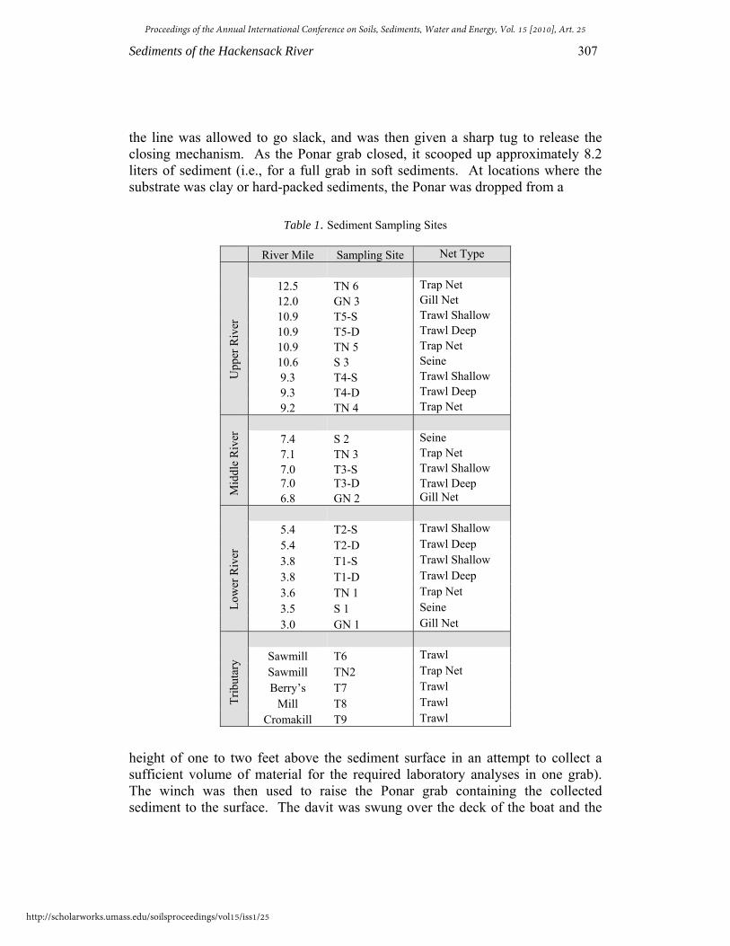
The locations sampled during the 2001-2003 fisheries study depicted in Figure 1 replicated the 1988 sites. Due to changes in site conditions during the intervening 13 years, two sampling sites, T9 and TN1, were slightly re-located from their original 1987-1988 locations. Sediment samples were collected by the MERI fisheries team once from each sampling location during the study. Three replicate samples were collected from each location, for a total of 78 sediment samples (river trawl locations were sampled at the shallow and deep end). Table 1 lists the sediment sampling sites, indicating lower Hackensack River segment, river mile or tributary, and fisheries gear type used at each location.

This report focuses solely on the chemical and textural analysis of the river bottom sediments. Sediments were characterized by parameters helpful for measuring ecological-risk and for making comparisons between sampling locations. In the sediments, heavy metal concentrations, grain size distribution and total organic carbon content were analyzed. “These data confirm whether samples were collected in depositional zones, as indicated by relatively higher carbon values and a higher percentage of fine-grained particles, and provide a qualitative indication of bioavailability. Depositional zones are areas of highest potential contamination” (Frasco, 1997). The metals arsenic, cadmium, chromium, copper, iron, lead, mercury, nickel and zinc were analyzed in all sediment samples.

2. MATERIALS AND METHODS

2.1 Field Methods

Sediment samples were collected using a standard 316-stainless steel Ponar grab sampler (sampling area of 0.05 m2, weight ~50 lbs.), deployed from a 21 foot Privateer work skiff via a davit equipped with a battery-operated winch. The collection of sediments for chemistry and textural analyses occurred over six days between July and December of 2003, with the majority of the samples collected in December. The first step of the sediment collection process was to anchor the boat above the sampling location. Water depth was ascertained using a Garmin model 160 Blue depthfinder. Next, the Ponar grab was arranged in the open position and it was slowly lowered through the water column using a sufficient length of 5/8 inch line until it contacted the sediment. Once the Ponar grab was on the bottom,




the line was allowed to go slack, and was then given a sharp tug to release the closing mechanism. As the Ponar grab closed, it scooped up approximately 8.2 liters of sediment (i.e., for a full grab in soft sediments. At locations where the substrate was clay or hard-packed sediments, the Ponar was dropped from a

Table 1. Sediment Sampling Sites

River Mile Sampling Site Net Type

Upp

er R

iver

12.5 TN 6 Trap Net 12.0 GN 3 Gill Net 10.9 T5-S Trawl Shallow 10.9 T5-D Trawl Deep 10.9 TN 5 Trap Net 10.6 S 3 Seine 9.3 T4-S Trawl Shallow 9.3 T4-D Trawl Deep 9.2 TN 4 Trap Net

Mid

dle

Riv

er

7.4 S 2 Seine 7.1 TN 3 Trap Net 7.0 T3-S Trawl Shallow 7.0 T3-D Trawl Deep 6.8 GN 2 Gill Net

Low

er R

iver

5.4 T2-S Trawl Shallow 5.4 T2-D Trawl Deep 3.8 T1-S Trawl Shallow 3.8 T1-D Trawl Deep 3.6 TN 1 Trap Net 3.5 S 1 Seine 3.0 GN 1 Gill Net

Trib

utar

y

Sawmill T6 Trawl Sawmill TN2 Trap Net Berry’s T7 Trawl

Mill T8 Trawl Cromakill T9 Trawl

height of one to two feet above the sediment surface in an attempt to collect a sufficient volume of material for the required laboratory analyses in one grab). The winch was then used to raise the Ponar grab containing the collected sediment to the surface. The davit was swung over the deck of the boat and the




Ponar grab was slowly lowered into a laboratory cleaned plastic tub (18.5 inches long x 14 inches wide x 7 inches high). Water overlying the sediment sample (if any) was slowly decanted through the screens at the top of the Ponar grab sampler and was discarded. The Ponar grab was then opened, releasing the collected sediments into the plastic tub. Any sediment adhering to the walls of the Ponar grab were scraped into the tub using a plastic scoop. The sediments were homogenized using the same plastic scoop, and were transferred to properly labeled, pre-cleaned, three-liter glass jar with a Teflon lid, and placed on ice in coolers for transfer to the Meadowlands Environmental Research Laboratory (MERI) laboratory. Three replicate samples were collected at each sampling location. Details regarding the collection location, date and time of sample collection, water depth, observations related to the sediments collected in each replicate sample, and any other pertinent observations were recorded in a field notebook, and are summarized in Table 2.

Table 2. Sediment Sampling

SITE Date

Sampled

Water Depth

(ft) Visual Description of

Sediment Additional Notes

GN1 12/04/03 ~15 grey sandy mud (Rep 2 produced a

sheen) Rep.1 required 3 grabs, and Rep 2

required 2 grabs

GN2 12/29/03 9 sticky grey clay Needed 2 grabs for each replicate

GN3 08/05/03 8.4 very soft black mud (consistency of

mayonnaise) Each replicate was a full grab

S1 12/04/03 4 mud underlain by sand & gravel

(mud produced a sheen) Replicate 1 required 3 grabs

S2 12/04/03 3 sandy mud Replicate 1 required 3 grabs

S3 12/12/03 2.5 soft black mud w/ thin brown surface

layer Each replicate was a full grab

T1 deep 12/18/03 16

stiff blackish-grey clay w/ a thin brown surface layer w/ sand & shell

hash Amphipods noted in samples T1 shallow 12/18/03 11 stiff grey clay

Each replicate was between 1/2 to 3/4 full

T2 deep 12/18/03 19 brown mud w/ some sand. Rep. 1

produced a slight sheen Replicates 2 & 3 required 2 grabs each T2 shallow 12/18/03 11

brown sandy mud w/ organic matter & silvery sheen Each replicate was ~1/4 full

T3 deep 12/18/03 15 soft black mud w/ thin (~1.5 - 2 inch

thick) brown surface layer Each replicate was a full grab




Table 2. Sediment Sampling (continued)

SITE Date

Sampled

Water Depth

(ft) Visual Description of

Sediment Additional Notes T3 shallow 12/18/03 4

soft black mud w/ thin brown surface layer Each replicate was a full grab

T4 deep 12/12/03 14 hard sticky grey clay Needed 2 grabs for each replicate T4 shallow 12/12/03 ~7 soft black mud Each replicate was a full grab

T5 deep 07/11/03 16.8 brownish-black mud (consistency of

mayonnaise) (no odor) Each replicate was a full grab

T5 shallow 07/11/03 8.3

black mud (consistency of mayonnaise) (with a slight chemical

odor) Replicates 1&2 were full grabs, Rep 3

was 3/4 full

T6 12/04/03 12 to 15 hard grey clay ~6 grabs needed for each replicate

T7 12/29/03 18 soft black mud w/ thin brown surface

layer, anaerobic odor, Phrag stalks Each replicate was a full grab

T8 12/29/03 9.8 brownish-grey soft mud w/ many Phragmites stalks, anaerobic odor

Amphipods and chironomid larvae noted

T9 12/29/03 10

very soft black mud (consistency of mayonnaise) w/ worm tubes on

surface Each replicate was a full grab

TN1 08/05/03 4.2 brownish-grey clayey mud Each replicate was ~3/4 full

TN2 08/05/03 5.1 greyish-black mud with thin brown

layer on top Each replicate was a full grab

TN3 12/04/03 5 blackish-grey mud w/ thin brown

surface layer Each replicate was a full grab

TN4 12/12/03 3 sticky black mud Each replicate was between 1/2 to 3/4

full

TN5 12/12/03 4 sticky black mud w/ a very soft top

layer Each replicate was a full grab

TN6 08/05/03 2 soft black mud (consistency of mayonnaise) (no odor or sheen) Each replicate was a full grab

The Ponar grab sampler was cleaned using site water and a hard-bristle scrub brush to remove any visible sediment before the next replicate sample was collected. After the third replicate sediment sample was collected at a particular sampling location, the Ponar grab sampler was decontaminated using a triple-step wash procedure that included an initial wash and scrub using site water, followed by an Alconox detergent wash/scrub and distilled water rinse, followed by a 10% nitric acid rinse, distilled water rinse, and finally an acetone rinse followed by a final distilled water rinse. The Ponar grab was then placed in a laboratory cleaned plastic tub, ready to be used at the next sediment collection location.




2.2 Physical Properties of Sediment

Sediment texture (particle-size), percent moisture and organic matter were determined for each sample in order to characterize the sediment and to help clarify the difference between site metal concentrations. Statistics performed to discern differences between sites normalized metal concentrations to the percentage of fine material contained in each sample. The American Society for Testing and Materials and (ASTM 2003) standard methods D 422 (particle-size) and D 2974 (moisture and organic matter) were utilized.

Figure 1. Map of Fisheries Inventory Sampling Locations




Appendix 1 contains the standard operating procedure for particle-size analysis. In summary:

1. The soil sample is dried at room temperature.

2. Sieve the ground sample through a No. 10 (2 mm) sieve using the Rotasift for 5 minutes. This material when weighed is the coarse fraction.

3. The material passing through the sieve is mixed with a dispersing agent until homogenized.

4. Transfer soil-water slurry (sample in dispersing agent) from its beaker into a glass sedimentation cylinder and fill to 1000mL with DI/distilled water.

5. Record both hydrometer (specific gravity) and temperature readings at intervals of 2, 5, 15, 30, 60, and 150 minutes after sedimentation begins.

6. When the hydrometer/temp readings are finished, pour the cylinder through a No. 230 (63 um) sieve. Dry the material retained on the No. 230 sieve at 105o C.

7. Once dried, break up aggregations and perform a final sieve analysis of the material through a No. 40 (425 um), No. 60 (250 um), and a No. 120 (125 um) sieve (simultaneously) for 20 minutes. Weigh and record the mass of material retained on each sieve and the material that passed through all three sieves. This is the mass of sandy material.

A calculator using Excel (Appendix 2 contains a sample spreadsheet) was devised to convert hydrometer readings to grain size classifications. This is necessary to distinguish between clay and silt size material (collectively referred to as % fines).

Table 3. Grain Size Classes

Sieve Grain Size Classification 4 4.75 mm Pebble

10 2.00 mm Granule 40 425 um Coarse Sand 60 250 um Medium Sand 120 125 um Fine Sand 230 62.5 um Very Fine Sand

<230 5 um Silt <5 um Clay

ASTM Method D 2974 describes the gravimetric determination of both moisture content and organic matter. Percent moisture was determined by drying




the sample for 16 hours at 105o C. Organic matter (ash content) was determined by igniting the oven dried sample from moisture content in a muffle furnace at 550 °C.

2.2 Metals Analysis

A sufficient amount of sediment (1-2 g wet weight, yielding 0.4-0.8 g dry weight) was oven-dried, weighed, and mineralized in 10 ml Trace Metal Grade HNO3 in Teflon bombs in a microwave digester. The resultant mineralized solution was boiled off to near dryness, restored to 25 ml volume with 1% HNO3, and divided. Twenty ml were used by the MERI laboratory for analysis of Cr, Cu, Cd, Fe and Pb by flame atomic absorption spectrophotometry (AAS). The remaining 5 ml were used by UMDNJ for Hg analysis by cold-vapor AA in a Bacharach MAS-50D mercury analyzer and for As analysis by hydride generation AA in a Perkin-Elmer 603 spectrophotometer. All metal analyses in 1988 were performed in the HMDC Laboratory (now MERI Laboratory) using AAS. Instrumentation in the MERI laboratory was upgraded in 2001.

One Standard Reference Material (SRM) was analyzed with every ten samples. Table 4 is a summary of the percent recovered, which ranged from 72.4% for Chromium to 103% for Cadmium in 2003, and 69.9% for Zinc to 120% for Cadmium in 1988. Arsenic, Mercury and Iron were not analyzed in 1988.

Table 4. Summary of SRM Recovery

Metal % Recovery 1988 2003 Arsenic 75.7 Cadmium 120 103 Chromium 105 72.4 Copper 92.4 99.7 Mercury 91.2 Lead 108 95.9 Nickel 115 95.6 Zinc 69.9 82.0 Iron 81.9

3. RESULTS AND DISCUSSION

3.1 Sediment Texture

Table 5 summarizes the average percent fine material (sum of the silt and clay fractions), organic matter (OM) and moisture content grouped by net type. On




average, the seine locations had the least amount of fine sediment. This is an artifact of the manner in which the sites were selected. Since the seine net was walked through the water and the net hauled up onto the shoreline at each seine location, sites that could not be easily traversed (i.e., those with thick mud) were not selected. Areas chosen as seine collection locations generally had a firm bottom (i.e., were lacking in fines). On the other hand, the trap net sites were selected to sample nearshore areas which were too muddy to seine. The trap nets were staked into mudflats at the selected locations that were close to shore, hence the high average percentage of fine material in the trap net samples. Intermediate between the seine and trap net locations were the gill net and trawl locations, which were generally located in deeper waters of the Hackensack River, or in the tributaries. The higher energy of the flowing river at some locations does not allow for the settlement of much fine material (e.g., GN1 and T2), while other sampling locations were clearly in areas of lower energy which were depositional in nature (e.g., T1 and T5).

Table 5. Net Type Averages of Physical Properties

Net Type # of Locations % Fines

% OM

% Moisture

Seines 3 40 7.7 50

Gill Nets 3 61 7.9 51

Trawls 14 70 9.8 60

Trap Nets 6 82 12.0 65

The surface area of particles increases as the size of particles decreases; as organic matter is often found as coatings on particles, it is reasonable for fine material and organic matter to co-vary as demonstrated by the net type averages. The moisture content of samples introduces the notion that opportunities for interchange between solid and liquid phases in the benthic environment are plentiful. In fact, the complexity of the system described by these parameters plays a strong role in the metal concentrations found in our samples.

Table 6 describes the texture of material sampled in the current and previous studies. Overall, the percentage of fines in the samples has remained relatively consistent; averaging 72% in 1988 and 69% in 2003. A plot of the data in Figure 2 reveals the temporal relationship in better detail. At Site T5 Deep, for example, fine material was relatively depleted in 1988 compared to 2003. This site is located in the channel of the River opposite the PSE&G Bergen Generating Station power plant; between 1988 and 2003 the cooling regime for this plant was converted from using river water to self contained cooling towers. This removed a thermal discharge plume which likely scoured the fine material from the river channel, providing a possible explanation for this change. Site S1 is also relatively depleted in fine material. The site is located along the bank of the river where a




strong current provides persistent scouring; but no change in conditions has occurred to explain the difference between the intervening years. Figure 2 also illustrates that one goal in the sampling design was met; collection sites were successfully replicated. This conclusion is supported by calculation of the population correlation coefficient between the two data sets: r = 0.73.

Table 6. Comparison of Fine Material Collected, 1988/2003

Sample Site 1988 2003 Difference GN1 11.5% 19.1% 7.6% GN2 73.0% 73.7% 0.7% GN3 98.2% 89.0% -9.2% S1 41.5% 1.80% -39.7% S2 40.3% 27.7% -12.6% S3 97.3% 91.3% -6.0% T1 (deep) 55.1% 70.6% 15.5% T1 (shallow) 56.4% 74.6% 18.2% T2 (deep) 17.6% 19.5% 1.9% T2 (shallow) 11.0% 40.2% 29.2% T3 (deep) 92.8% 87.5% -5.3% T3 (shallow) 91.0% 81.2% -9.8% T4 (deep) 88.9% 60.9% -28.0% T4 (shallow) 93.9% 68.6% -25.3% T5 (deep) 14.8% 84.7% 69.9% T5 (shallow) 96.7% 79.6% -17.1% T6 94.8% 76.6% -18.2% T7 94.6% 84.6% -10.0% T8 91.4% 84.0% -7.4% T9 92.5% 86.4% -6.1% TN1 76.3% 83.6% 7.3% TN2 94.8% 86.5% -8.3% TN3 96.0% 78.6% -17.4% TN4 89.4% 76.7% -12.7% TN5 77.6% 80.1% 2.5% TN6 84.8% 85.6% 0.8% Average 72.0% 68.9% -3.1%

The percentage of fine material helps describe the sedimentary character of the estuary, both spatial and temporal. The sampling sites covered nine miles of the river and the major tributaries that are within the Hackensack Meadowlands




District. Grouping the river sampling sites spatially can reveal differences between the lower, middle and upper part of the river within the District. Refer to Table 1 for the grouping of sites. Note that each river segment is separated by at least 1.5 river miles. Because of the strong influence of net type on sediment characteristics, an attempt was made to include a sampling from each net type in each segment. Exceptions are the absence of a gill net in the upper part of the river and a seine in the tributaries.

Figure 2. Plot of Site Textures

Figure 3A compares the average of fine percentages found in the tributaries and river in 1988 and 2003: Tributaries contain finer material then the river; the river hasn’t changed during the 15 year interval between sampling; and there has been a 12% reduction in the percentage of fine material found in tributary samples. The composition of fine material is a function of hydrodynamics. As energy in the water column dissipates, finer material is deposited. The River would naturally have higher energy, with finer material being carried until deposition occurs in mudflats, along the shorelines and in the tributaries. Because the relative amount of fine material is very dynamic, it is difficult to draw conclusions from this data; for example, the increased energy from storm events can redistribute fine material in the short term that would mask long term changes in the River.

Figure 3B is a comparison between the average of fine percentages found in the three segments of the river in 1988 and 2003: The average percentage found in

0%

10%

20%

30%

40%

50%

60%

70%

80%

90%

100%

GN1GN2

GN3 S1 S2 S3

T1 (dee

p)

T1 (sha

llow)

T2 (dee

p)

T2 (sha

llow)

T3 (dee

p)

T3 (sha

llow)

T4 (dee

p)

T4 (sha

llow)

T5 (dee

p)

T5 (sha

llow) T6 T7 T8 T9

TN1TN2

TN3TN4

TN5TN6

Sample

Perc

ent F

ines Series1

Series219882003




the lower river has increased 13%; the middle part of the river has decreased by 13%; and the upper part of the river has remained relatively unchanged (2% decrease). Appendices 3 and 4 contain the complete grain size analysis for sediments collected in 1988 and 2003.

Figure 3A. Spatial Distribution of Percent Fines: River vs. Tributaries

Figure 3B. Spatial Distribution of Percent Fines: River Segments

3.2 METALS

The metals and organic chemicals selected for analysis are contaminants known to bioaccumulate. The organics and mercury bioconcentrate, i.e., accumulating to higher levels (typically an order of magnitude) with each trophic level, making them of special concern (Weis 2005). The discussion which follows will include a description of the spatial distribution of metal concentrations collected in 2003

0%10%20%30%40%50%60%70%80%90%

100%

1 2

Series1

Series2

0%10%20%30%40%50%60%70%80%90%

100%

1 2 3

Series1Series2

1988 2003

1988 2003

Lower Middle Upper




and the factors affecting that distribution; and a comparison between data collected in 2003 and 1988 using sediment quality criteria as a measure of ecosystem quality. A complete listing of concentrations obtained in 2003 and 1988 appears in Appendices 5 and 6.

There are no absolute chemical concentrations that correspond to sediment toxicity, but “Effects Range Low” (ERL) and “Effects Range Median” (ERM) values are used as guidelines in assessing sediment contamination. ERM is the median concentration of a contaminant observed to have adverse biological effects in the literature studies examined (Long et al 1995). A more protective indicator of contaminant concentration is the ERL criteria, which is the 10th percentile concentration of a contaminant represented by studies demonstrating adverse biological effects in the literature. Ecological effects are not likely to occur at contaminant concentrations below the ERL criterion (USEPA 2004, p. 12).

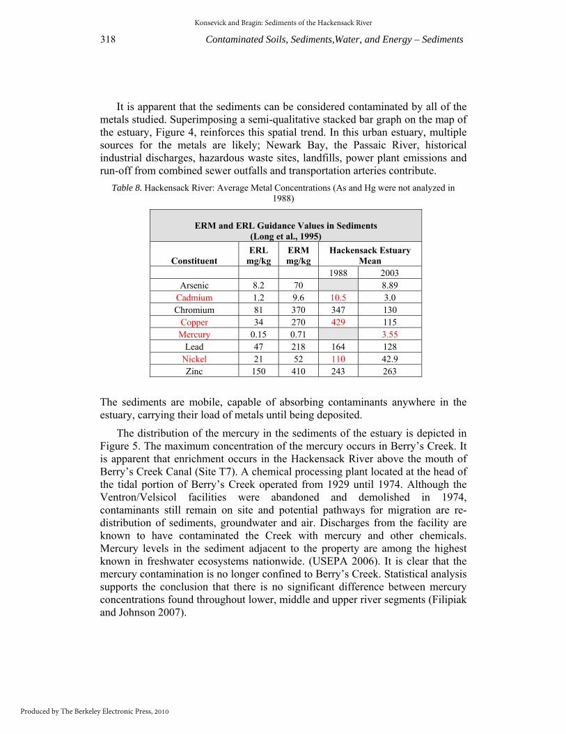
Table 7 describes qualitative ratings for sites based on ERM and ERL criteria. Based on the EPA’s sediment contamination assessment criteria, the ecological condition of the Hackensack River estuary sediments in 2003 was Poor; the average concentration of one contaminant, mercury, exceeds the ERM. Table 8 provides a comparison of average metal concentrations obtained in 1988 and 2003 to the ERM and ERL criteria. Metals which exceeded the ERM criteria are printed in red. In 1988, three additional metals cadmium, copper and nickel exhibited concentrations that would have exceeded the ERM criteria. The improvement in sediment quality in the 15 years between studies is depicted in the table as the high concentrations of cadmium, copper and nickel are no longer experienced in these estuarine sediments.

Table 7. Criteria for Assessing Sediment Contaminants by Site (USEPA 2004, p. 17)

Rating Criteria Good No ERM concentrations are exceeded, and less than five ERL

concentrations are exceeded. Fair Five or more ERL concentrations are exceeded Poor An ERM concentration is exceeded for one or more contaminants.

Six of the 21 river samples, collected primarily at sites below the mouth of Berrys Creek, exhibit Good sediment quality: the mercury ERM is not exceeded and less than five ERLs are exceeded (See Table 9). None of the tributary sites meet this criteria. Other contaminants that exceed ERM criteria in individual samples are cadmium, lead, nickel and zinc. The average concentration of all of the metals exceed ERL criteria; 60% of the sampling sites exceed more than five ERLs.




It is apparent that the sediments can be considered contaminated by all of the metals studied. Superimposing a semi-qualitative stacked bar graph on the map of the estuary, Figure 4, reinforces this spatial trend. In this urban estuary, multiple sources for the metals are likely; Newark Bay, the Passaic River, historical industrial discharges, hazardous waste sites, landfills, power plant emissions and run-off from combined sewer outfalls and transportation arteries contribute.

Table 8. Hackensack River: Average Metal Concentrations (As and Hg were not analyzed in 1988)

The sediments are mobile, capable of absorbing contaminants anywhere in the estuary, carrying their load of metals until being deposited.

The distribution of the mercury in the sediments of the estuary is depicted in Figure 5. The maximum concentration of the mercury occurs in Berry’s Creek. It is apparent that enrichment occurs in the Hackensack River above the mouth of Berry’s Creek Canal (Site T7). A chemical processing plant located at the head of the tidal portion of Berry’s Creek operated from 1929 until 1974. Although the Ventron/Velsicol facilities were abandoned and demolished in 1974, contaminants still remain on site and potential pathways for migration are re-distribution of sediments, groundwater and air. Discharges from the facility are known to have contaminated the Creek with mercury and other chemicals. Mercury levels in the sediment adjacent to the property are among the highest known in freshwater ecosystems nationwide. (USEPA 2006). It is clear that the mercury contamination is no longer confined to Berry’s Creek. Statistical analysis supports the conclusion that there is no significant difference between mercury concentrations found throughout lower, middle and upper river segments (Filipiak and Johnson 2007).

ERM and ERL Guidance Values in Sediments (Long et al., 1995)

Constituent ERL

mg/kg ERM mg/kg

Hackensack Estuary Mean

1988 2003 Arsenic 8.2 70 8.89

Cadmium 1.2 9.6 10.5 3.0 Chromium 81 370 347 130

Copper 34 270 429 115 Mercury 0.15 0.71 3.55

Lead 47 218 164 128 Nickel 21 52 110 42.9 Zinc 150 410 243 263




Table 9 represents the average metal concentration of three replicates collected at each site. The organization of the table by river miles and tributaries with coloration of concentrations exceeding the ERL sediment criteria (See Table 8), allows for a visual representation of spatial trends. The distribution of ERL exceedences (five or more per site) suggests that with two exceptions, S-2 at mile 7.4 and T-4 Deep at mile 9.3, the river north of mile 7.0 is likely to suffer negative ecological effects.

Figure 4. Visual Depiction of metal spatial trend

Figure 5. Visual Depiction of mercury spatial trend

NickleLeadMercuryCopperChromiumCadmium

CopperChromiumCadmiumArsenic




Table 9. Hackensack River metal concentrations obtained in 2003 Values exceeding the ERL are typed in boldface; values exceeding the ERM are bolded and

italicized.

Metals (mg/kg) Arsenic Cadmium Chromium Copper Mercury Lead Nickel Zinc Iron ERL 8.2 1.2 81 34 0.15 47 21 150 ERM 70 9.6 370 270 0.71 218 52 410

Sampling Sites

River Mile

GN 1 3.0 5.13 0.80 68.9 33.9 1.11 61.5 16.2 101 12472 S 1 3.5 10.4 0.42 96.1 46.6 0.85 73.7 57.8 113 34720

TN 1 3.6 17.1 2.48 145 118 2.57 148 41.7 230 29198 T1-S 3.8 7.01 0.14 23.2 14.5 0.09 27.3 25.2 59.2 26463 T1-D 3.8 8.76 0.13 20.6 11.2 0.05 22.6 22.6 56.4 27471 T2-S 5.4 3.68 0.29 32.4 11.8 0.20 22.7 10.8 54.7 11997 T2-D 5.4 3.58 0.46 76.0 19.5 0.43 39.4 14.0 68.6 12139 GN 2 6.8 8.26 0.34 33.3 24.9 0.38 29.1 28.1 82.0 34512 T3-S 7.0 9.65 1.69 121 99.1 2.65 113 41.9 213 33966 T3-D 7.0 8.16 1.45 108 92.5 2.22 105 40.2 210 30418 TN 3 7.1 8.92 1.62 130 99.3 4.19 129 40.5 236 34945 S 2 7.4 5.68 0.90 69.1 47.4 2.86 58.0 22.4 130 19859

TN 4 9.2 11.8 5.95 218 177 5.99 193 59.8 390 36687 T4-S 9.3 11.1 8.43 240 228 8.65 227 74.3 437 38166 T4-D 9.3 5.79 0.36 21.3 13.8 0.09 45.3 20.2 61.2 24987 S 3 10.6 9.64 2.95 165 158 4.36 168 49.9 359 37232

T5-S 10.9 13.4 9.88 278 255 6.34 287 76.2 660 35524 T5-D 10.9 9.87 7.28 228 220 5.79 231 71.8 522 36034 TN 5 10.9 9.11 3.90 178 175 4.35 182 53.8 384 36923 GN 3 12.0 9.63 5.30 190 270 4.67 205 51.2 527 37760 TN 6 12.5 10.1 5.08 168 237 4.65 282 52.3 494 37772 TN2 Sawmill 9.33 2.03 190 270 2.06 205 51.2 527 37760 T6 Sawmill 6.36 0.13 123 106 0.20 130 41.1 244 32817 T7 Berry’s 13.8 13.05 23 13 20.8 22 25.8 66 29304 T8 Mill 22.8 1.93 297 237 3.41 227 73.4 536 38060 T9 Cromakill 11.6 2.19 170 133 3.28 141 52.2 283 38843

3.3 Sediment Metal Behavior

We can look to the relative concentration of total carbon and fine grained particles to discern why the metals reside where they do. Concentration distributions presented to show patterns of regional contaminant distributions and metal co-variances imply common sources or behaviors (Mecray et al 2001). Table 10 displays the Pearson product-moment coefficient (R2) which depicts the strength of the correlation of the values of independent variables obtained at each sampling




site. With the exception of iron and arsenic, the sediment correlation matrix displays the close affinity of all of the metals. A general linear model was used to measure the relationship between each of the metals as independent or predictor variables and other metal as dependent or criterion variable (Filipiak and Johnson 2007). The significant model equations for each of the metals confirmed the strong interaction between the metals (Filipiak and Johnson 2007). Because correlation does not imply causation, it cannot be inferred from this information that the metals share a common source. It is more likely that their observed distributions result from the influence of hydrodynamics reflected by sediment texture and organic content.

Table 10. Sediment Correlation Matrix (R2)

* Correlation coefficients > 0.77

Arsenic Cadmium Chromium Copper Iron Lead Mercury Nickel Zinc River mile

% Fines

Cadmium 0.47 Chromium 0.58 0.93* Copper 0.50 0.91* 0.92* Iron 0.63 0.55 0.63 0.66 Lead 0.56 0.91* 0.94* 0.96* 0.65 Mercury 0.43 0.89* 0.93* 0.88* 0.60 0.90* Nickel 0.67 0.80* 0.87* 0.78* 0.83* 0.82* 0.76* Zinc 0.47 0.94* 0.93* 0.99* 0.65 0.97* 0.89* 0.80* River mile 0.13 0.77* 0.71 0.85* 0.62 0.79* 0.81* 0.60 0.85* % Fines 0.55 0.54 0.54 0.65 0.70 0.62 0.58 0.47 0.63 0.61 % TOC 0.62 0.85* 0.89* 0.92* 0.79* 0.95* 0.87* 0.82* 0.92* 0.80* 0.79*

Particulate size and resulting total surface area available for adsorption are both important factors in adsorption processes… smaller particles can both be more widely dispersed by water and can also serve as sites of enhanced adsorption (John and Leventhal 1995 p. 13). In this estuary dominated by the tidal regime, depositional environments occur when energy dissipates. One would expect the percent of fine material to increase as the distance increases from the mouth of the river; a moderate correlation (R2 = 0.61) between % fines (silt and clay fraction) and river mile does exist. The strength of the correlation between the metals and % fines is moderate as well (average R2 = 0.59). A confounding factor which diminishes the strength of the river mile/ percent fines correlation relates to the differing substrate requirements for the four net-types used for sampling fish which provided the sites for sediment collections as well (Table 5).




A better predictor of metal concentrations in the sediments appears to be the amount of organic matter present in the sediments. In organic carbon-rich sediments, trapped interstitial fluids can commonly form a strongly reducing (anoxic) environment. The sediment samples in this study averaged almost 60% water. Low redox potential in this environment can promote sulfate reduction and sulfide mineral deposition. During diagenesis, much of the potentially toxic metals, such as arsenic, cadmium, copper, mercury, lead, and zinc, can form insoluble sulfides; a change to an oxidizing environment caused by disturbance of the sediment and exposure to the atmosphere or with the influx of oxygenated (sea) water can result in rapid reaction of this anoxic sediment and thereby release significant proportions of these metals (John and Leventhal 1995 p. 13). The sulfate/sulfide mechanism appears to effect metal concentrations, helping to explain the enrichment in the upper reaches of the river and depletion as oxygenated sea water interacts the organic matter in sediments.

3.4 1988/2003 Comparison

Between 1988 and 2003, the average sediment concentration of cadmium, chromium, copper, lead and nickel was reduced by between 22% and 71%; zinc concentrations remained relatively constant (8% increase). This dramatic improvement suggests a natural attenuation process is burying contaminated sediments with cleaner material. Perhaps the naturally high background concentration of zinc found in this region provides a continuous supply of this metal to the sediments.

Table 11. Metal Comparison 1988/2003

Average Metal Concentrations (mg/kg) Metal 1988 2003 Difference Cadmium 10.5 3.0 -71% Chromium 347 130 -63% Copper 429 115 -73% Lead 164 128 -22% Nickel 110 42.9 -61% Zinc 243 263 +8%

Statistical analysis was performed on the sediment metal concentrations as well (Filipiak and Johnson 2007). Three sites, S1, S3 and TN5, were not included in the year to year comparison. S3 was excluded because there was no data in 1988; it had been identified as S4. S1 and TN5 were excluded as the site identification was recorded incorrectly. To test whether there were significant different between studies done in 1987-88 and 2003 a paired t test was used. The justification for using the paired t experimental design was the methodology of having samples collected at approximately the same geographical locations where




the only factor is the time in between collections (Filipiak and Johnson 2007).

Significant difference in concentrations was found for the following metals in sediments when comparing 1987-88 and 2003 using a paired t-test:

• Cadmium (Cd), levels higher for 1987-88

• Chromium (Cr), levels higher for 1987-88

• Copper (Cu), higher for 1987-88

• Lead (Pb), higher for 1987-88.

When the sites were grouped according to their location in the main river or tributaries, the following metals exhibited significant differences in the main river:

• Cadmium (Cd), higher for 1987-88

• Copper (Cu), higher for 1987-88

• Lead (Pb), higher for 1987-88

The main river levels of Chromium, Nickel and Zinc did not have a statistically significant change between 1987-88 and 2003. In the tributaries, there were no significant differences for any of the metals studied.

Statistics were also applied to the Lower, Middle and Upper segments of the Hackensack River (see Table 1 and Figure 1). The only statistically significant result was the higher value of cadmium concentrations in the Lower River in 1987-88 compared to 2003.

4. CONCLUSIONS

Sampling and analytical methods applied to the sediment study of 2003 successfully replicated the 1988 effort, allowing for spatial and temporal comparisons between physical and chemical properties. The ecological quality of the Hackensack River Estuary was discerned using guidance criteria applied to metal concentrations.

The texture of bottom sediments has not changed greatly during the 15 year interval between studies and the sediment quality has clearly improved. Between 1988 and 2003, the average sediment concentration of cadmium, chromium, copper, lead and nickel was reduced by between 22% and 71%. However, since 60% of the sampling sites exceed more than five ERLs the estuary continues to exhibit metal contamination.




Mercury concentrations once thought to be confined to Berry’s Creek, have now reached all parts of the estuary. Since Mercury was not determined in the 1989 study, it was not possible to determine trends over time.

Finally, the majority of the metals seem to be correlated. This correlation however does not conclusively show that they share a common source. The study indicates that their observed distributions are also closely related to sediment texture and organic content.

5. REFERENCES

ASTM International, 2003. Standard Test Method for Particle-Size Analysis of Soils, D422-63(2002). Bragin, A. B., Misuik, J., Woolcott, C. A., Barrett, K. R, and Jusino-Atresino, R. 2005. A Fishery Resource

Inventory of the Lower Hackensack River within the Hackensack Meadowlands District A Comparative Study 2001-2003 vs. 1987-1988. New Jersey Meadowlands Commission, Meadowlands Environmental Research Institute, Lyndhurst, NJ 07071.

Filipiak, Karolina A., and Johnson, K., 2007. Analysis of the Sediment Data from the Lower Hackensack River, Abstract and presentation to the 2007 Meadowlands Symposium, New Jersey Meadowlands Commission, Meadowlands Environmental Research Institute, Lyndhurst, NJ 07071.

Frasco, Barry, 1997. Memorandum: Present use of draft 1991 NJDEP guidance for sediment quality evaluations, October 1997 update.

Goeller, A. F. III, 1989 Heavy metals and radionuclides in sediments of the Hackensack River, New Jersey. Master of Science Thesis, Rutgers University, Newark, New Jersey.

HMDC. 1989. Inventory of Fishery Resources of the Hackensack River within the jurisdictional Boundary of the Hackensack Meadowlands Development Commission from Kearny, Hudson County, to Ridgefield, Bergen County, New Jersey.

John, David A and Joel S. Leventhal, 1995. BIOAVAILABILITY OF METALS. Ch. 2 in: Preliminary compilation of descriptive geoenvironmental mineral deposit models Edward A. du Bray, Editor. U.S. DEPARTMENT OF THE INTERIOR U.S. GEOLOGICAL SURVEY Open-File Report 95-831, Denver, Colorado.

Long, E.R., D.D. MacDonald, S.L. Smith, and F.D. Calder, 1995. Incidence of adverse biological effects within ranges of chemical concentrations in marine and estuarine sediments. Environmental Management 19(1):81–97.

Mecray, Ellen L., M. R. Buchholtz ten Brink, and S. Shah. 2001 Metal Distributions in the Surface Sediments of Long Island Sound. U.S. Department of the Interior, U.S. Geological Survey, URL: http://pubs.usgs.gov/of/2000/of00-304/htmldocs/chap06/index.htm in: Georeferenced Sea-Floor Mapping and Bottom Photography in Long Island Sound, Edited By Valerie F. Paskevich and Lawrence J. Poppe.

United States Environmental Protection Agency, Office of Research and Development Office of Water, December 2004. National Coastal Condition Report II, Washington, DC 20460. EPA-620/R-03/002 http://www.epa.gov/owow/oceans/nccr2/.

United States Environmental Protection Agency Region 2 Superfund, VENTRON/VELSICOL, NEW JERSEY NPL Site Fact Sheet EPA ID# NJD980529879. http://www.epa.gov/region02/superfund/npl/0200674c.pdf Accessed 3/16/2006

Weis, Peddrick, 2005. Contaminants in Fish of the Hackensack Meadowlands, NJMC Report, 28 pp.




APPENDIX 1. Grain-Size Analysis SOP

Standard Test Method for Particle-Size Analysis of Soils, D422-63(2002). ASTM International, 2003.

(Nicole Quinn, MERI)

Procedure:

Expose the soil sample (about 130g out of jar for silt/clay soils, about 200g for sandy soils) to air at room temperature until dry. Use the blower under the hood. This could take 2-7 days.

Break up aggregations in a mortar with a rubber-covered pestle, trying not to crush the grains.

Sieve the ground sample through a No. 10 (2 mm) sieve using the Rotasift for 5 minutes.

Break up aggregations retained on No. 10 sieve, using mortar and pestle. Sieve the ground material again through the No. 10 sieve for 5 minutes.

After sieving the sample twice through the No. 10 sieve, remove the sieve and wash with DI/distilled water anything retained on the sieve. Put this sieve in the oven to dry at a temp. of 100 – 105 degrees Celsius. This is the coarse material.

Get a 250mL beaker and a spatula and measure out 50g into the beaker for silt/clay soils and 100g for sandy soils. Use at least 32g for silt/clay and 82g for sandy soils. Use the PB3002-S DeltaRange scale.

Add 125mL of the dispersing solution (40g/L sodium hexametaphosphate) to the beaker and stir until homogenized. Cover with parafilm, label, and leave for at least 16 hours.

To make more dispersing solution, measure 40g of sodium hexametaphosphate and add to about 800mL DI/distilled water in a 1000mL beaker. Place on stir plate, and using stir bar, mix for about 20 minutes or until homogenized.

Remove the sieve with the coarse material from oven when the sample is dry and sieve it for 5 minutes through both a No. 10 and a No. 4 sieve, simultaneously. Weigh and record the masses for each sieve. These are the masses of coarse material for the sample. Use the PB221S Sartorius scale.

After 16 hours, begin the hydrometer readings for the samples. Use the same 151H hydrometer that was used throughout this project, for which a composite correction has already been made.




Transfer soil-water slurry (sample in dispersing agent) from its beaker into a glass sedimentation cylinder and fill to 1000mL with DI/distilled water. Rinse all soil from beaker into cylinder. Label the cylinders. Only two tests can be run at a time, and it is possible to finish four in a day.

Use a rubber stopper to cap the cylinder. Record both hydrometer (specific gravity) and temperature readings at intervals of 2, 5, 15, 30, 60, and 150 minutes after sedimentation begins. Hold both ends of the cylinder and mix for one minute. Setting down the cylinder is the beginning of sedimentation. Record your start time.

When you have finished the hydrometer/temp readings for the sample, pour the cylinder through a No. 230 (63 um) sieve over the sink and run tap water though it until clear. Dry the material retained on the No. 230 sieve in an aluminum weighing dish in the oven at 105 degrees Celsius. This will take about 1.5 – 2 days for most samples to completely dry.

Once dried, break up aggregations in mortar with rubber-covered pestle. Perform a final sieve analysis of the material through a No. 40 (425 um), No. 60 (250 um), and a No. 120 (125 um) sieve (simultaneously) for 20 minutes. Weigh (on the Sartorius scale) and record the mass of material retained on each sieve and the material that passed through all three sieves. This is the mass of sandy material.




APPENDIX 2. GRAIN-SIZE CALCULATOR

PARTICLE-SIZE ANALYSIS OF SOILS ASTM D 422

Start by recording data from notebook or worksheet.

Hit [F9] to calculate.

Save to a new file name and repeat.

Sample # 78816

Location GN2-

3 Weight (g) 50.0

Temperature C 21.0

K 0.014

Sieve Analysis Size Classification and

% Sieve Weight (g) Pebble 0.00%

4 0.000 Granule 0.25%

10 0.124 Coarse

Sand 0.00%

40 0.000 Medium

Sand 5.36% 60 2.681 Fine Sand 4.03%

120 2.013 Very Fine

Sand 0.00% 230 0.000 Silt 62.6%

<230 45.18 Clay 27.8%




Hydrometer

Analysis Time (T)

Hydrometer reading

% in Suspension

Depth L L/T

Diameter (D) Ln D

2 1.020 65.0% 11.0 5.500 0.032 -

3.439

5 1.017 55.2% 11.8 2.360 0.021 -

3.862

15 1.014 45.5% 12.6 0.840 0.013 -

4.378

30 1.012 39.0% 13.1 0.437 0.009 -

4.705

60 1.011 35.7% 13.4 0.223 0.006 -

5.041

150 1.009 29.2% 13.9 0.093 0.004 -

5.480

Silt diameter Ln Trend

Coefficient

0.005-

5.298 0.308




APPENDIX 3. SEDIMENT SAMPLE TEXTURES 2003

Location Pebble 4 MM

Granule 2 MM

Coarse Sand 0.5

MM

Medium Sand 0.25 MM

Fine Sand 0.125 MM

Very Fine Sand

0.0625 MM

Silt 0.005 MM

Clay < 0.005 MM

TN1-1 0.72% 0.31% 0.96% 1.37% 0.03% 21.0% 33.3% 42.4% TN1-2 0.34% 0.71% 0.00% 0.00% 0.00% 0.00% 47.5% 51.4% TN1-3 0.00% 0.33% 0.45% 2.07% 0.03% 20.8% 38.0% 38.3% S1-1 16.4% 11.3% 33.8% 17.5% 0.01% 18.2% 1.76% 1.01% S1-2 29.5% 12.1% 31.3% 9.21% 0.06% 17.4% 0.31% 0.18% S1-3 21.7% 19.4% 17.1% 9.78% 0.02% 29.6% 1.31% 1.06% GN1-1 0.02% 0.50% 1.50% 12.9% 15.9% 50.6% 9.15% 9.54% GN1-2 1.13% 1.07% 2.51% 13.6% 0.01% 65.1% 9.87% 6.65% GN1-3 0.05% 0.67% 2.92% 12.8% 0.01% 61.4% 12.0% 10.2% T1-1 Deep 6.85% 2.11% 1.17% 3.68% 0.02% 35.4% 25.8% 24.9% T1-2 Deep 0.00% 0.00% 0.46% 1.97% 0.01% 25.4% 21.4% 50.8% T1-3 Deep 0.00% 0.00% 2.95% 3.29% 5.00% 0.0% 42.3% 46.5% T1-1 Shallow 0.00% 0.00% 0.36% 2.46% 0.03% 11.9% 26.3% 58.9% T1-2 Shallow 1.01% 2.52% 3.29% 2.33% 0.06% 15.5% 28.5% 46.7% T1-3 Shallow 7.41% 2.15% 3.22% 3.46% 0.02% 20.5% 23.3% 40.0% TN2-1 0.00% 0.06% 1.17% 1.93% 3.06% 13.0% 29.6% 51.3% TN2-2 0.00% 0.04% 0.17% 0.36% 0.00% 4.39% 35.2% 59.9% TN2-3 0.00% 0.15% 0.72% 1.40% 0.09% 14.1% 25.2% 58.3% S2-1 13.3% 5.55% 6.26% 10.2% 0.04% 23.6% 22.2% 18.9% S2-2 27.4% 8.64% 0.00% 27.0% 18.8% 12.2% 3.4% 2.62% S2-3 27.4% 8.14% 8.22% 5.85% 1.53% 12.9% 12.1% 23.9% GN2-1 5.43% 0.70% 1.42% 8.90% 0.03% 17.4% 21.3% 44.8% GN2-2 0.00% 0.35% 0.61% 3.45% 0.02% 30.9% 27.8% 36.9% GN2-3 0.00% 0.25% 0.00% 5.36% 4.03% 0.00% 23.9% 66.4% T2-1 Deep 11.9% 1.89% 10.2% 26.7% 0.01% 49.1% 0.17% 0.07% T2-2 Deep 4.07% 2.55% 9.79% 12.7% 0.02% 16.8% 42.2% 11.9% T2-3 Deep 3.69% 1.87% 21.9% 30.4% 0.05% 38.0% 3.17% 0.88% T2-1 Shallow 0.11% 0.51% 8.30% 2.39% 0.01% 83.7% 3.6% 1.44% T2-2 Shallow 2.48% 0.75% 0.55% 2.10% 0.01% 69.4% 16.8% 7.92% T2-3 Shallow 0.00% 0.01% 1.64% 2.56% 0.02% 86.5% 8.22% 1.10% TN3-1 0.00% 0.07% 12.3% 9.87% 6.94% 21.0% 28.2% 21.5% TN3-2 0.60% 0.02% 0.36% 0.37% 0.00% 5.29% 31.7% 61.7% TN3-3 0.99% 0.17% 0.37% 0.38% 0.00% 5.43% 15.8% 76.9%





Granule 2 MM

Coarse Sand 0.5

MM

Medium Sand 0.25 MM

Fine Sand 0.125 MM

Very Fine Sand

0.0625 MM

Silt 0.005 MM

Clay < 0.005 MM

S3-1 0.00% 0.30% 0.42% 1.02% 0.01% 3.34% 18.7% 76.2% S3-2 0.07% 0.56% 1.39% 2.76% 0.01% 6.03% 31.9% 57.3% S3-3 0.00% 0.48% 1.24% 2.92% 0.03% 5.57% 25.5% 64.2% GN3-1 0.00% 0.00% 11.6% 0.79% 0.05% 1.66% 45.7% 40.2% GN3-2 0.00% 0.18% 3.22% 0.64% 0.00% 1.55% 51.0% 43.4% GN3-3 0.00% 0.00% 7.02% 1.10% 0.04% 5.25% 42.1% 44.4% T3-1 Deep 0.00% 0.00% 2.21% 3.22% 0.08% 17.4% 20.1% 57.0% T3-2 Deep 0.00% 0.29% 0.27% 0.29% 0.00% 6.47% 26.8% 65.9% T3-3 Deep 0.22% 0.07% 0.19% 0.33% 0.02% 6.55% 22.7% 69.9% T3-1 Shallow 0.00% 12.6% 0.16% 0.39% 0.03% 6.04% 25.4% 55.4% T3-2 Shallow 0.00% 0.14% 0.26% 0.42% 0.02% 7.15% 27.3% 64.7% T3-3 Shallow 0.00% 0.00% 1.50% 3.88% 0.03% 23.7% 28.4% 42.6% TN4-1 0.00% 0.01% 1.76% 0.87% 0.02% 4.31% 26.3% 66.8% TN4-2 0.00% 0.02% 13.7% 0.84% 0.23% 4.08% 27.1% 54.0% TN4-3 0.00% 0.00% 3.74% 8.69% 0.07% 31.5% 19.7% 36.3% T4-1 Deep 0.00% 0.18% 0.19% 1.53% 0.03% 36.6% 24.9% 36.6% T4-2 Deep 0.00% 0.13% 1.90% 2.23% 0.04% 46.7% 22.1% 26.9% T4-3 Deep 0.19% 0.05% 0.22% 1.95% 0.02% 25.5% 30.2% 41.8% T4-1 Shallow 0.00% 0.00% 5.41% 8.22% 0.06% 30.2% 14.0% 42.1% T4-2 Shallow 0.00% 0.11% 3.04% 0.98% 0.01% 4.83% 32.0% 59.0% T4-3 Shallow 0.00% 0.00% 8.01% 6.98% 0.08% 26.3% 18.6% 40.1% TN5-1 0.00% 0.00% 9.64% 6.26% 0.13% 26.9% 18.6% 38.4% TN5-2 0.00% 0.00% 0.00% 8.85% 2.07% 0.00% 23.8% 65.3% TN5-3 0.00% 0.07% 3.68% 1.84% 0.47% 0.00% 34.4% 59.6% T5-1 Deep 0.00% 0.00% 5.14% 1.02% 0.01% 5.10% 45.0% 43.7% T5-2 Deep 0.00% 0.06% 1.10% 1.12% 0.01% 8.29% 34.8% 54.6% T5-3 Deep 0.00% 0.21% 4.45% 2.81% 0.09% 16.6% 28.1% 47.8% T5-1 Shallow 0.00% 1.95% 1.46% 1.68% 0.17% 6.93% 41.6% 46.2% T5-2 Shallow 0.00% 0.00% 8.96% 3.26% 0.26% 14.4% 32.0% 41.1% T5-3 Shallow 0.00% 0.07% 7.61% 1.99% 0.01% 12.4% 35.8% 42.2% TN6-1 1.47% 0.08% 9.00% 2.38% 0.02% 6.80% 35.1% 45.2% TN6-2 0.00% 0.06% 1.21% 0.79% 0.29% 5.82% 27.0% 64.8% TN6-3 0.01% 0.25% 3.14% 4.04% 0.24% 7.54% 41.1% 43.7% T6-1 0.00% 0.96% 6.29% 4.34% 1.76% 0.00% 22.9% 63.7% T6-2 2.98% 1.90% 6.82% 10.1% 0.02% 20.3% 20.3% 37.5% T6-3 0.00% 0.06% 0.03% 2.04% 0.02% 12.4% 11.5% 74.0%





Granule 2 MM

Coarse Sand 0.5

MM

Medium Sand 0.25 MM

Fine Sand 0.125 MM

Very Fine Sand

0.0625 MM

Silt 0.005 MM

Clay < 0.005 MM

T7-1 0.00% 0.04% 4.77% 0.92% 0.01% 5.24% 41.7% 47.4% T7-2 1.52% 5.12% 9.30% 2.31% 0.02% 7.78% 46.7% 27.3% T7-3 0.56% 0.53% 2.23% 1.04% 0.33% 4.47% 37.7% 53.1% T8-1 2.38% 4.07% 2.44% 1.37% 0.04% 5.10% 40.2% 44.4% T8-2 0.08% 1.03% 1.40% 1.74% 0.01% 8.56% 31.7% 55.4% T8-3 3.34% 4.53% 4.38% 2.14% 0.47% 4.91% 51.0% 29.3% T9-1 0.02% 0.07% 5.73% 2.43% 0.01% 6.64% 53.6% 31.5% T9-2 0.19% 0.15% 2.72% 1.85% 0.01% 5.91% 44.4% 44.8% T9-3 0.00% 0.14% 4.26% 2.10% 0.02% 8.70% 43.7% 41.1%




APPENDIX 4. SEDIMENT SAMPLE TEXTURES (PERCENTAGE) 1988


Granule 2 MM

Very Coarse Sand 1 MM

Coarse Sand 0.5 MM

Medium Sand 0.25 MM

Fine Sand 0.125 MM

Very Fine Sand

0.0625 MM

Silt and Clay

< 0.0625 MM

TN1 0 0.2 1.6 2.8 6.1 7.7 5.3 76.3

S1 8 6.4 6.2 10.4 12.8 12.2 4.6 39.4

GN1 0 0.3 0.3 0.7 22.2 58.5 6.5 11.5

T1 Deep 3.6 3.7 1.7 2 5.9 16.2 11.8 55.1

T1 Shallow 0.32 0.5 0.4 1.3 3.8 20.9 16.4 56.4

TN2 0 0.3 0.8 0 0.4 2.2 1.5 94.8

S2 0.7 1 2.2 4.4 8.8 24.4 18 40.3

GN2 0 0.7 0 0.8 10 8.6 6.7 73

T2 Deep 0.1 1.9 2 10.1 27.8 30.8 9.8 17.6

T2 Shallow 54.1 6.5 2.9 3.5 8.2 10.1 3.6 11

TN3 0 0.2 0.7 1.3 0.2 0.9 0.7 96

S3 0 0.1 0.5 0 0.2 1.3 0.5 97.3

GN3 0 0 0 0 0.2 0.1 1.5 98.2

T3 Deep 0 0 0.8 0 0.1 1.6 4.7 92.8

T3 Shallow 0 0.7 0.1 0 0.4 2.1 5.8 91

TN4 0 0.7 0.3 0 0 1.5 2.8 89.4

T4 Deep 0 0 0.4 0 0.2 2.1 8.3 88.9

T4 Shallow 0 0.7 0.3 0 0.1 1.7 3.3 93.9

TN5 0 0 0.7 0 1 14.8 5.8 77.6

T5 Deep 0 0.3 3.5 7.9 29.8 38.3 5.4 14.8

T5 Shallow 0 0.1 0 0 0.1 0.3 2.8 96.7

TN6 0 0.3 0.5 1.6 1 7.5 4.3 84.8

T6 0 0 0.6 0 0.5 2.1 2.1 94.8

T7 0 0.2 0.8 0.2 0.3 1.7 2.3 94.6

T8 0 0.1 0.3 0 0.4 5.8 2 91.4

T9 0 0.1 0.8 0.1 1 2.9 2.6 92.5

Note: Percentages reflect the results obtained from one sample collected at each location.




APPENDIX 5. METAL CONCENTRATIONS OF SEDIMENTS COLLECTED IN 2003 (MG/KG DRY WT.)

Collection T.O.C. % Fines METALS (ug/g) Dry Weight

Site - Rep. # Date (%) (silt & clay) As Cd Cr Cu Hg Pb Ni Zn Fe

T5 Shallow-1 7/11/03 N.D. 87.8 12.3 7.36 134 203 4.64 230 52.0 469 37348 T5 Shallow-2 7/22/03 13.7 73.1 13.3 11.7 316 294 5.84 306 95.9 738 35332 T5 Shallow-3 7/22/03 13.2 77.9 14.5 10.6 384 268 8.55 327 80.6 773 33892

T5 Deep-1 7/22/03 14.3 88.7 10.0 4.22 142 189 4.28 185 55.1 436 37593 T5 Deep-2 7/22/03 15.9 89.4 9.3 6.18 145 197 4.43 202 63.3 453 38317 T5 Deep-3 7/22/03 15.9 75.8 10.3 11.4 398 274 8.66 306 96.8 675 32193

GN3-1 8/5/03 13.1 85.9 9.1 5.24 190 258 4.85 144 50.2 521 39472 GN3-2 8/5/03 12.8 94.4 8.4 5.03 198 261 4.46 221 47.3 505 35780 GN3-3 8/5/03 11.8 86.6 11.4 5.63 183 289 4.69 250 56.1 555 38029

TN6-1 8/5/03 16.4 80.3 10.0 5.58 174 234 4.56 239 55.2 510 38999 TN6-2 8/5/03 15.8 91.8 10.1 4.94 173 243 4.55 241 49.0 516 38106 TN6-3 8/5/03 13.6 84.8 10.2 4.71 159 234 4.83 366 52.7 455 36209

TN1-1 8/5/03 9.39 75.6 11.9 1.39 124 101 2.49 125 38.3 196 28208 TN1-2 8/5/03 10.3 99.0 18.0 3.92 146 114 2.58 161 43.0 244 27904 TN1-3 8/5/03 10.7 76.3 21.4 2.13 166 140 2.63 158 43.9 251 31481

TN2-1 8/5/03 9.42 80.8 9.40 1.63 119 104 1.77 115 37.8 239 32867 TN2-2 8/5/03 10.2 95.0 9.30 2.52 127 106 2.31 136 46.2 243 31953 TN2-3 8/5/03 9.65 83.6 9.30 1.96 123 109 2.11 139 39.2 251 33632

GN1-1 12/4/03 2.17 18.7 4.85 0.83 62.9 35.4 1.43 52.7 16.5 98 13214 GN1-2 12/4/03 4.50 16.5 4.50 0.71 72.1 26.1 0.73 51.5 13.1 86 10119 GN1-3 12/4/03 5.54 22.1 6.04 0.88 71.8 40.2 1.19 80.5 19.0 118 14085

S1-1 12/4/03 3.71 2.77 10.7 0.29 118 36.4 0.30 54.1 71.9 91 35598 S1-2 12/4/03 4.76 0.49 11.2 0.43 80.6 45.7 1.28 76.9 42.0 116 39712 S1-3 12/4/03 8.15 2.37 9.2 0.54 89.9 57.8 0.98 90.2 59.6 133 28849

T6-1 12/4/03 6.04 86.7 6.11 0.14 24.1 13.1 0.10 25.4 28.1 71.2 30114 T6-2 12/4/03 4.86 57.8 6.37 0.09 17.0 11.2 0.45 15.2 19.6 50.0 22551 T6-3 12/4/03 6.09 85.4 6.59 0.16 27.1 15.8 0.05 24.1 29.7 76.1 35248

S2-1 12/4/03 5.35 41.1 7.23 1.03 97.5 65.2 2.81 81.4 30.1 175 24612 S2-2 12/4/03 4.41 5.98 3.98 0.67 46.0 30.0 2.06 39.6 15.7 89.1 14593 S2-3 12/4/03 4.66 36.0 5.84 0.99 63.7 47.0 3.72 52.8 21.5 126 20371

TN3-1 12/4/03 10.5 49.7 8.38 1.61 125 98.3 5.03 117 38.8 225 33847 TN3-2 12/4/03 7.04 93.4 9.06 1.62 127 100 3.36 143 40.3 241 34899 TN3-3 12/4/03 10.6 92.7 9.32 1.62 137 99.3 4.18 126 42.2 242 36088

TN5-1 12/12/03 12.5 57.0 9.01 4.27 184 183 4.47 189 56.8 401 36467 TN5-2 12/12/03 12.7 89.1 9.16 3.24 163 162 3.79 170 50.4 386 38544 TN5-3 12/12/03 12.7 93.9 9.15 4.18 187 181 4.79 187 54.3 363 35759

S3-1 12/12/03 12.5 94.9 9.79 3.01 179 157 5.11 177 49.6 373 37568




Collection T.O.C. % Fines METALS (ug/g) Dry Weight

Site - Rep. # Date (%) (silt & clay) As Cd Cr Cu Hg Pb Ni Zn Fe

S3-2 12/12/03 12.7 89.2 9.33 3.31 158 169 4.32 163 51.0 347 36712 S3-3 12/12/03 12.8 89.8 9.79 2.52 159 147 3.66 163 49.2 356 37417

T4 Deep-1 12/12/03 6.52 61.5 6.28 0.20 19.7 13.1 0.11 27.6 22.2 58 24479 T4 Deep-2 12/12/03 5.74 49.0 7.90 0.18 19.8 12.9 0.15 30.5 17.0 54 26222 T4Deep-3 12/12/03 6.89 72.1 3.18 0.71 24.6 15.5 0.02 77.7 21.5 71 24260

T4 Shallow-1 12/12/03 13.0 56.1 10.7 8.01 241 248 9.58 232 74.6 426 39234 T4 Shallow-2 12/12/03 11.9 91.0 11.6 8.87 226 210 8.69 223 75.3 451 37175 T4Shallow-3 12/12/03 13.5 58.6 11.1 8.41 253 225 7.66 225 72.8 434 38090

TN4-1 12/12/03 13.6 93.0 11.7 5.38 214 185 5.23 187 60.2 396 37472 TN4-2 12/12/03 15.1 81.2 12.4 6.49 224 180 6.24 199 62.0 396 39010 TN4-3 12/12/03 11.1 56.0 11.2 5.97 217 165 6.49 193 57.1 377 33579

T1 Shallow-1 12/18/03 7.10 85.2 8.80 0.10 22.4 13.8 0.06 22.1 26.8 63.5 29156 T1 Shallow-2 12/18/03 5.10 75.3 6.71 0.20 27.2 16.3 0.16 36.4 25.6 64.6 24839 T1 Shallow-3 12/18/03 8.50 63.3 5.51 0.14 20.0 13.4 0.05 23.5 23.0 49.5 25396

T1 Deep-1 12/18/03 6.79 50.7 8.89 0.11 18.8 12.4 0.13 25.3 21.7 48.1 28642 T1 Deep-2 12/18/03 6.01 72.2 8.02 0.12 20.7 9.66 0.00 20.9 25.5 61.0 27684 T1 Deep-3 12/18/03 4.00 88.8 9.38 0.17 22.4 11.5 0.03 21.8 20.6 59.9 26087

T2 Shallow-1 12/18/03 2.48 5.03 3.44 0.30 34.9 10.9 0.20 14.9 10.3 52.6 11720 T2 Shallow-2 12/18/03 2.00 24.7 3.85 0.20 31.6 11.0 0.21 25.9 10.8 57.5 12256 T2Shallow-3 12/18/03 2.60 91.0 3.74 0.35 30.7 13.4 0.19 27.4 11.3 54.0 12015

T2 Deep-1 12/18/03 2.61 0.25 3.79 0.43 83.8 17.1 0.40 24.6 13.1 66.9 12197 T2 Deep-2 12/18/03 2.63 54.1 3.30 0.34 45.0 15.2 0.35 48.9 11.7 52.8 9580 T2 Deep-3 12/18/03 1.92 4.06 3.64 0.63 99.3 26.2 0.55 44.6 17.2 86.0 14639

T3 Shallow-1 12/18/03 9.05 80.8 9.41 1.68 113 96.6 2.53 111 42.6 206 35249 T3 Shallow-2 12/18/03 10.2 92.0 9.18 1.74 127 103 2.74 115 42.1 214 33548 T3 Shallow-3 12/18/03 10.6 70.9 10.3 1.65 124 97.8 2.69 114 41.1 220 33101

T3 Deep-1 12/18/03 10.4 77.1 8.47 1.29 109 97.3 1.83 104 40.2 224 30968 T3 Deep-2 12/18/03 10.2 92.7 7.62 1.46 104 88.6 2.29 99.2 38.6 197 28276 T3 Deep-3 12/18/03 9.88 92.6 8.39 1.60 111 91.5 2.56 112 41.9 208 32010

GN2-1 12/29/03 7.03 66.1 9.36 0.45 41.7 33.7 0.55 35.0 31.3 98.3 37439 GN2-2 12/29/03 4.78 64.6 10.1 0.27 23.7 17.2 0.30 25.4 29.1 76.7 34499 GN2-3 12/29/03 5.12 90.4 5.38 0.31 34.4 23.9 0.30 27.0 23.9 71.0 31598

T7-1 12/29/03 9.09 89.0 13.9 11.57 308 240 15.09 234 73.2 519 35445 T7-2 12/29/03 19.0 74.0 14.2 13.70 287 224 25.24 215 72.6 535 45747 T7-3 12/29/03 12.5 90.8 13.3 13.88 296 247 22.19 231 74.4 554 32987

T8-1 12/29/03 21.0 84.6 11.4 1.98 168 136 3.53 138 50.4 289 39307 T8-2 12/29/03 15.6 87.2 1.30 1.45 160 130 2.65 136 52.7 276 36831 T8-3 12/29/03 20.4 80.2 55.6 2.35 181 133 4.04 149 53.5 283 40390

T9-1 12/29/03 16.4 85.1 12.0 2.04 158 144 3.08 162 53.0 328 39216 T9-2 12/29/03 16.5 89.2 11.2 1.97 159 149 3.33 144 50.6 271 46105

T9-3 12/29/03 16.1 84.8 11.5 2.56 157 145 3.44 152 51.0 337 35251




T.O.C. % Fines METALS (ug/g) Dry Weight

(%) (silt & clay) As Cd Cr Cu Hg Pb Ni Zn Fe

MIN 1.92 0.25 1.30 0.09 17 10 0.00 15 10.3 48 9580

MAX 21.01 99.0 55.6 13.9 398 294 25.2 366 96.8 773 46105

AVG 9.78 68.9 9.64 3.05 130 115 3.55 128 42.9 263 31095

ST DEV 4.69 28.1 6.26 3.47 87 88 4.30 86 20.3 185 8756

* The T.O.C. values shown are the mean of two samples. + The T.O.C. value shown is the mean of three samples.




APPENDIX 6. METAL CONCENTRATIONS OF SEDIMENTS COLLECTED IN 1988 (MG/KG DRY WT.)

Sample N Ni Cu Pb Cd Zn Cr T1 (shallow) 4 37.3 ± 4.3 176 ± 10.8 151.3 ± 39.8 2.8 ± 0.5 140.5a 256.5 ± 26.1

T1 (deep) 2 49.5 371 28.5 1.7 114b 35

T2 (shallow) 2 86.5 1128.5 101 2.9 367b 71

T2 (deep) 2 127.5 836.5 196 3.7 402b 251

T3 (shallow) 2 22.5 121.5 116.5 2.9 96b 115

T3 (deep) 2 38 163.5 119.5 3.8 112b 145.5

T4 (shallow) 3 61.7 ± 2.4 303 ± 11.5 235.3 ± 46.5 8.9 ± 0.7 225b 430.3 ± 95.1

T4 (deep) 3 60.3 ± 6.3 271 ± 9.9 219.7 ± 25.2 8.0 ± 1.1 180a 302.7 ± 104.9

T5 (shallow) 2 92.5 235.5 212.5 13 307 313.5

T5 (deep) 3 306.3 ± 27.6 1063 ± 216.0 328.3 ± 88.3 8.7 ± 2.1 481.3 ± 59.7 821.3 ± 80.0

T6 3 71.0 ± 6.5 175.7 ± 9.0 23.7 ± 3.7 1.7 ± 0.3 109.7 ± 71.7 39.7 ± 27.1

T7 1 49 172 125 8.5 118 195

T8 1 52 110 25 2.8 75 25

T9 2 91.5 491 324 13.5 563.5 1196

GN1 3 502.3 ± 327.7 1917 ± 378.2 215.3 ± 40.4 4.2 ± 0.4 569.3 ± 78.2 920.3 ± 424.8

GN2 2 84 259.5 190.5 6.2 187 284.5

GN3 2 133 586.5 258 13.9 497.5 415.5

TN1 3 128.3 + 61.5 166 ± 7.1 115.7 ± 15.8 3.9 ± 1.0 100.7± 4.1 309.7 ± 136.7TN2 2 63.5 156.5 100.5 4.7 134 189 TN3 1 61 156 106 4.9 129 198 TN4 1 52 151 97 4.7 123 151 TN5 5 124.2 ± 40.3 229.4 ± 16.8 174.6 ± 24.5 5.5 ± 1.1 171.4 ± 53.5 459 ± 175.9 TN6 2 133 350 233.5 9.2 276.5 366 SI 3 218 16.5 529 + 28.5 164.3 + 21.3 5.9 + 0 332.7 + 102.8 917.3 + 175.1S2 2 124 424.5 154 8 271.5 285 S3/S4 1 87 602 249 120 241 334

MIN 22.5 110 23.7 1.70 75.0 25.0

MAX 502 1917 328 120 569 1196

AVG 110 429 164 10.5 243 347

ST DEV 100 412 82.5 22.6 153 299



chemical characteristics of sediment of the lower hackensack river, new jersey

Documents