chapter 9 signals & systems
TRANSCRIPT

Chapter 9
Signals & Systems
Contents9.1 Introduction to transforms: Fourier, Laplace, and Z . . . . . . . . . . . . . . . . . . . . . 9-2
9.1.1 The relation of the Laplace and Z transforms to the Fourier transform . . . . . . . . . . 9-39.1.2 The remarkable utility of such transforms . . . . . . . . . . . . . . . . . . . . . . . . . . 9-3
9.2 Laplace transform methods . . . . . . . . . . . . . . . . . . . . . . . . . . . . . . . . . . . . 9-49.2.1 The Laplace Transform of derivatives and integrals of functions . . . . . . . . . . . . . . 9-69.2.2 Using the Laplace Transform to solve unforced linear dierential equations . . . . . . . 9-79.2.3 Continuous-time (CT) transfer functions . . . . . . . . . . . . . . . . . . . . . . . . . . . 9-7
9.3 Z transform methods . . . . . . . . . . . . . . . . . . . . . . . . . . . . . . . . . . . . . . . 9-139.3.1 The Z Transform of translated sequences . . . . . . . . . . . . . . . . . . . . . . . . . . 9-139.3.2 Using the Z Transform to solve unforced linear dierence equations . . . . . . . . . . . 9-149.3.3 Discrete-time (DT) transfer functions . . . . . . . . . . . . . . . . . . . . . . . . . . . . . 9-159.3.4 Reconciling the Laplace and Z transforms . . . . . . . . . . . . . . . . . . . . . . . . . . 9-19
9.4 Frequency-domain analyses and lters . . . . . . . . . . . . . . . . . . . . . . . . . . . . . 9-239.4.1 The Bode plot . . . . . . . . . . . . . . . . . . . . . . . . . . . . . . . . . . . . . . . . . . 9-239.4.2 Low-pass, high-pass, band-pass, and band-stop lters . . . . . . . . . . . . . . . . . . . . 9-28
Exercises . . . . . . . . . . . . . . . . . . . . . . . . . . . . . . . . . . . . . . . . . . . . . . . . . . 9-36
By way of introduction, we begin this chapter, in §9.1, by presenting briefly the three essential classes oftransforms at the heart of signal analysis: Fourier, Laplace, and Z . The Fourier transform, which comes infour forms appropriate for either continuous signals defined throughout the domain of interest or discretesignals defined only at regularly-spaced intervals over the domain of interest, and for signals defined on eitherinfinite domains that is1, t ∈ (−∞,∞) or bounded domains that is, t ∈ [0, T ), is built on sinusoidal basisfunctions, eiωt = cos(ωt) + i sin(ωt), as studied in depth in §5 of NR.
Before discussing the Laplace and Z transforms and their extensive utility in control theory, it is helpfulto make this discussion a bit more concrete by considering the ODE modeling of a handful of simple physicalsystems (a.k.a. “plants”), as reviewed in §7, as we will return to these motivating examples at several pointsin this presentation. Note also that the realization of various ODEs of interest (particularly as “controllers”) aselectric circuits is considered in §10.
1As in §5 of NR, the physical coordinate over which such transforms may be applied may be interpreted as time or space, and isdenoted without loss of generality in the present chapter as t; see also footnote 19 in §5.5 of NR.
9-1
Renaissance Robotics (v.2021-09-01) Chapter 9: Signals & Systems
The Laplace transform, which is appropriate for the analysis of continuous signals on semi-infinitedomains t ∈ [0,∞), as well as for the analysis of the dierential systems that govern their evolution fromgiven initial conditions at t = 0, is built on exponential basis functions, est, and is developed in §9.2.
The Z transform, which is appropriate for the analysis of discrete signals on semi-infinite domainstk ∈ 0, h, 2h, 3h, . . ., as well as for the analysis of the dierence systems that govern their evolution fromgiven initial conditions around t0 = 0, is built on polynomial basis functions, zk−1, and is developed in §9.3.
The use of Fourier transforms in signal analysis is then extended significantly in §9.4.
9.1 Introduction to transforms: Fourier, Laplace, and ZRecall first the tetralogy of Fourier transforms:
The forward and inverse infinite Fourier series transform [see §5.2 of NR], defined for continuous signalsu(t) on bounded domains t ∈ [0, T ) with ωn = 2πn/T for n ∈ . . . ,−2,−1, 0, 1, 2, . . ., are defined by
un =1
T
∫ T
0
u(t)e−iωnt dt ⇔ u(t) =∞∑
n=−∞une
iωnt, (9.1a)
the forward and inverse infinite Fourier integral transform [see §5.3 of NR], defined for continuous signalsu(t) on infinite domains t ∈ (−∞,∞) with ω ∈ (−∞,∞), are defined2 by
u(ω) =1
2π
∫ ∞−∞
u(t)e−iωt dt ⇔ u(t) =
∫ ∞−∞
u(ω)eiωtdω, (9.1b)
the forward and inverse finite Fourier series transform [see §5.4 of NR], defined for discrete signalsuk = u(tk) on bounded domains tk = kh for k = 0, . . . , N − 1 and h = T/N with3 ωn = 2πn/T forn ∈ −N/2, . . . , N/2, are defined by
un =1
N
N−1∑k=0
uke−iωntk ⇔ uk =
N/2∑n=−N/2
uneiωntk , (9.1c)
and the forward and inverse finite Fourier integral transform [as developed in Exercise 5.2 of NR], defined fordiscrete signals uk = u(tk) on infinite domains tk = kh for k = . . . ,−2,−1, 0, 1, 2, . . . with ω ∈ (−π/h, π/h),are defined by
u(ω) =h
2π
∞∑k=−∞
uke−iω tk ⇔ uj =
∫ π/h
−π/hu(ω)eiω tj dω. (9.1d)
Similarly, the forward and inverse Laplace transform [developed in §9.2] are defined by
U(s) =
∫ ∞0
u(t)e−stdt ⇔ u(t) =1
2πi
∫ γ+i∞
γ−i∞U(s)estds, (9.2)
and the forward and inverse Z transform [developed in §9.3] are defined by
U(z) =∞∑k=0
ukz−k ⇔ uk =
1
2πi
∮Γ
U(z)zk−1 dz. (9.3)
2Recall from Footnote 10 in §5.4 of NR that there are alternative definitions of the Fourier integral, so dierent authors will placethe factor of 2π in these formulae in dierent ways.
3Note in particular the discussion in §5.5 of NR of the peculiar component of this signal at the Nyquist frequency ωN/2 = πN/T .
9-2
Renaissance Robotics (v.2021-09-01) Chapter 9: Signals & Systems
9.1.1 The relation of the Laplace and Z transforms to the Fourier transformAt the outset, note that the Laplace transform at right in (9.2) is simply a representation, or “expansion”, of acontinuous function u(t) on t ∈ [0,∞) as a linear combination of a set of exponential basis functions est withthe coeicient function U(s) as weights. Similarly, the Z transform at right in (9.3) is simply a representationof a discrete function uk on k = 0, 1, 2, . . . as a linear combination of a set of polynomial basis functions zk−1
with the coeicient function U(z) as weights. The Laplace and Z transforms are thus remarkably similar tothe corresponding Fourier transforms (9.1b) and (9.1d), respectively, which similarly represent continuous anddiscrete functions on infinite domains as a linear combination of a set of complex exponential basis functionswith the Fourier coeicients as weights. Indeed, noting the definition of the Laplace transform in (9.2) and theinfinite Fourier integral expansion in (9.1b), it follows that
U(s) =
∫ ∞0
u(t)e−stdt
u(ω) =1
2π
∫ ∞−∞
u(t)e−iωt dt
⇒ u(ω) =1
2πU(iω) if u(t) = 0 for t < 0. (9.4)
Similarly, noting the definition of the Z transform in (9.3) and the finite Fourier integral expansion in (9.1d), itfollows that
U(z) =∞∑k=0
ukz−k
u(ω) =h
2π
∞∑k=−∞
uke−iω tk
⇒ u(ω) =h
2πU(eiωh) if uk = 0 for k < 0. (9.5)
9.1.2 The remarkable utility of such transformsThe utility of the Fourier transform in the identification and analysis of the various sinusoidal components of asignal at dierent spatial frequencies or temporal wavenumbers should already be well familiar to the reader.(Indeed, any aspiring audiophile is already well familiar with the need to route the “low-frequency sinusoidalcomponents” of an audio signal to a woofer, to route the “high-frequency sinusoidal components” of an audiosignal to a tweeter, and to dampen the “highest-frequency sinusoidal components” of an audio signal associatedwith noise, which can come from a variety of sources; the Fourier transform simply makes this decompositionof a signal into sinusoidal components at dierent frequencies mathematically precise.)
The Laplace and Z transforms are similarly natural for the analysis of the evolution of continuous-time(CT) systems and discrete-time (DT) systems from initial conditions, governed by dierential equations anddierence equations respectively. As such transform methods are centrally based on an abstraction (the tem-poral frequency ω or spatial wavenumber k in the case of the Fourier transforms, the exponential scaling s inthe case of the Laplace transform, and the base of the polynomial expansion, z, in the case of the Z transform),they require a bit of analysis before their utility is fully apparent; §9.2 and §9.3 are intended to make this utilityevident.
It should be noted at the outset, however, that all of these transforms are linear: that is, if X and Y arethe (Fourier, Laplace, or Z) transforms of x and y, then αX + βY is the corresponding transform of αx + βy.Further, all of these transforms are invertible: that is, knowledge of the untransformed variable x over theappropriate region of the physical domain is suicient to reconstruct the transformed variable X over theabstracted domain, and knowledge of the transformed variableX over the appropriate region of the abstracteddomain is suicient to reconstruct the untransformed variable x over the physical domain. These two pointsare essential to the practical utility of analysis, filtering, and control techniques based on such transforms.
9-3
Renaissance Robotics (v.2021-09-01) Chapter 9: Signals & Systems
9.2 Laplace transform methodsThe (one-sided) Laplace transform F (s) of a continuous-time (CT) signal f(t) is, in general, defined as
F (s) = limε→0
∫ ∞−ε
f(t)e−stdt ,∫ ∞
0−f(t)e−stdt. (9.6)
In this text, we restrict all functions f(t) to which we apply the Laplace transform to be at least le-continuousat the origin [that is, f(−ε) → f(0) as ε → 0 with ε > 0]. Accordingly, when the need for a CT unit impulsearises, we construct it as the large λ limit of the one-sided function4 δλ,m(t) (described in §5.3.4 of NR, form ≥ 1). In this restricted5 seing, the Laplace transform may be defined (see LePage 1961) more simply as
F (s) =
∫ ∞0
f(t)e−stdt. (9.7a)
Given a le-continuous f(t) for t ≥ 0, we will define F (s) via (9.7a). The inverse Laplace transform is
f(t) =1
2πi
∫ γ+i∞
γ−i∞F (s)estds, (9.7b)
where the real number γ is chosen such that the vertical line of the contour given in the above integral is to theright of all of the singularities6 of F (s) in the complex plane s.
Verification that (9.7b) in fact represents the inverse of the relationship expressed in (9.7a) is straightforward,by substituting (9.7a) into the RHS of (9.7b), substituting s = γ + ik, applying Fubini’s theorem (see Footnote2 in §5.2.1 of NR), and noting that, for suiciently large γ, f(t) is indeed recovered:
1
2πi
∫ γ+i∞
γ−i∞
[ ∫ ∞0
f(t′) e−st′dt′]est ds = lim
K→∞
1
2πi
∫ K
−K
[ ∫ ∞0
f(t′) eγ(t−t′)eik(t−t′)dt′]
i dk
= limK→∞
∫ ∞0
f(t′)eγ(t−t′)[ ∫ K
−K
1
2πeik(t−t′)dk
]dt′ =
∫ ∞0
[f(t′) eγ(t−t′)] δ(t− t′) dt′ = f(t),
where the definition of the Dirac delta given in §5.2.2 of NR has been applied in the second line. The reasonthat the eγ(t−t′) factor, for suiciently large positive γ, is required by this formula is to ensure that the termg(t′) = [f(t′) eγ(t−t′)] decays to zero exponentially as t′ →∞, which allows us to swap the order of the integralsusing Fubini’s theorem and obtain the result that
∫∞0g(t′) δ(t− t′) dt′ = g(t).
As discussed further below, the forward and inverse transforms expressed by (9.7) are immensely usefulwhen solving dierential equations (in CT). By (9.7a), knowing f(t) for t ≥ 0, one can define F (s) on anappropriate contour. Conversely, by (9.7b), knowing F (s) on an appropriate contour, one can determine f(t)for t ≥ 0. Before demonstrating further why such a transformation is useful, we first mention that, in practice,you don’t actually need to compute the somewhat involved integrals given in (9.7) in order to use the Laplacetransform eectively. Rather, it is suicient to reference a table listing some Laplace transform pairs in a fewspecial cases, as shown in Table 9.1a. Note also the following:
Fact 9.1 The Laplace transform is linear; that is, superposition holds, and thus if the Laplace transforms ofa(t) and b(t) are A(s) and B(s), then the Laplace transform of c(t) = a(t) + b(t) is C(s) = A(s) +B(s).
Fact 9.2 If the Laplace transform of f(t) isF (s), then the Laplace transform of the exponentially scaled functiong(t) = e−atf(t) is G(s) =
∫∞0f(t)e−(s+a)tdt = F (s + a), and the Laplace transform of the delayed function
g(t) = f(t− d) is G(s) =∫∞
0f(t− d)e−stdt =
∫∞−d− f(t)e−s(t+d)dt = e−dsF (s).
4That is, rather than the small σ limit of the two-sided function δσ(t) described in §5.3.3 of NR.5This “restriction” is said to be technical; that is, it narrows the precise mathematical seing in which the transform definition
may be used, but in application does not limit the practical problems to which the transform may, when used correctly, be applied.6That is, the contour of integration in (9.7b) is chosen to the right of all points s for which |F (s)| → ∞ as s→ s in (9.7a).
9-4

Renaissance Robotics (v.2021-09-01) Chapter 9: Signals & Systems
f(t) (for t > 0) F (s)
eat 1/(s− a)
t eat 1/(s− a)2
t2 eat 2/(s− a)3
tp eat (for integer p ≥ 0) p!/(s− a)p+1
1 [i.e., f(t) = h0(t)] 1/s
t 1/s2
tp (for integer p ≥ 0) p!/sp+1
δλ,m(t) −−−→λ→∞
1
δλ,m(t− d) (for d ≥ 0) −−−→λ→∞
e−ds
d[δλ,m(t)]/dt , δ′(t) −−−→λ→∞
s
d2[δλ,m(t)]/dt2 , δ′′(t) −−−→λ→∞
s2
eat cos(bt)s− a
(s− a)2 + b2
eat sin(bt)b
(s− a)2 + b2
cos(bt) s/(s2 + b2)
sin(bt) b/(s2 + b2)
cosh(bt) s/(s2 − b2)
sinh(bt) b/(s2 − b2)
fk (for k = 0, 1, . . .) F (z)
ck z/(z − c)k ck c z/(z − c)2
k2ck c z(z + c)/(z − c)3
k3ckcz(z2 + 4 c z + c2)
(z − c)4
kpck (for p > 0) Li−p(c/z)
1 [i.e., fk = h0k] z/(z − 1)
k z/(z − 1)2
kp (for integer p > 0) Li−p(1/z)
δ0k 1
δdk (for integer d) 1/zd
ck cos(θk)z[z − c cos(θ)]
z2 − 2 c z cos(θ) + c2
ck sin(θk)z c sin(θ)
z2 − 2 c z cos(θ) + c2
ck h1k c/(z − c)(k − 1) ck h2k c2/(z − c)2
(k − 2)(k − 1) ck h3k 2 c3/(z − c)3
(k − 3)(k − 2)(k − 1) ck h4k 6 c4/(z − c)4
(k − p) · · · (k − 1) ck hp+1,k p! cp+1/(z − c)p+1
Table 9.1: Tables of (le) some Laplace transform pairs, as considered in §9.2, and (right) some Z transformpairs, as considered in §9.3. Note that the (le-continuous) CT functions f(t) = 0 for t ≤ 0, and that the DTfunctions fk = 0 for integer k < 0. The CT unit impulse in this work is taken as the large λ limit (under theintegral sign!) of the one-sided function δλ,m(t) for some integer m ≥ 1. The polylogarithm Lin(z) and theDT Heaviside step function hdk are defined in (B.77) and (B.79b) of NR.
Note in Table 9.1a that the Laplace transform of the delay function, f(t) = δλ,m(t − d) in the limit oflarge λ for d > 0, is F (s) = e−ds; this is not a rational function7 of s, which turns out to be inconvenient.The following Padé approximation of the Laplace transform of a delay, valid for small values of |ds|, is thusconvenient to use in its stead
e−ds ≈ Fn(s) ,
∑nk=0(−1)kck(ds)
k∑nk=0 ck(ds)
k, ck =
(2n− k)!n!
(2n)! k! (n− k)!. (9.8)
The formula for the coeicients in the above approximation may be verified by considering the expression
[∑n
k=0 ak(ds)k]e−ds ≈ [
∑nk=0 bk(ds)
k],
7A rational function of s is a polynomial in s divided by a polynomial in s.
9-5
Renaissance Robotics (v.2021-09-01) Chapter 9: Signals & Systems
inserting the Taylor-series expansion for e−ds, expanding, and matching as many coeicients of like powers of(ds) as possible. The resulting rational approximations of the delay function e−ds, for n = 1, 2, and 4, are
F1(s) =1− ds/21 + ds/2
, F2(s) =1− ds/2 + (ds)2/12
1 + ds/2 + (ds)2/12, F4(s) =
1− ds/2 + 3(ds)2/28− (ds)3/84 + (ds)4/1680
1 + ds/2 + 3(ds)2/28 + (ds)3/84 + (ds)4/1680.
9.2.1 The Laplace Transform of derivatives and integrals of functionsAssume f(t) is smooth and bounded and define f (1)(t) = df(t)/dt = f ′(t). Then, by integration by parts, theLaplace transform of f (1)(t) is given by
F (1)(s) =
∫ ∞0
f (1)(t)e−stdt = lima→∞
∫ a
0
f (1)(t)e−stdt
= lima→∞
[e−saf(a)− f(0) + s
∫ a
0
e−stf(t)dt]
= sF (s)− f(0)
(9.9a)
for <(s) > 0. Similarly, if f (2)(t) = d2f(t)/dt2 = f ′′(t) and f (n)(t) = dnf(t)/dtn, then
F (2)(s) =
∫ a
0
f (2)(t)e−stdt = . . . = s2F (s)− sf(0)− f (1)(0), (9.9b)
F (n)(s) =
∫ a
0
f (n)(t)e−stdt = . . . = snF (s)− sn−1f(0)− sn−2f (1)(0)− . . .− f (n−1)(0). (9.9c)
Thus, if f (1)(t) = df(t)/dt, then F (1)(s) = sF (s)−f(0). Conversely, by integration, it therefore follows that, iff(t) =
∫ t0f (1)(t′)dt′, and thus f(0) = 0, then F (s) = 1
sF (1)(s). We thus arrive at the most useful interpretation
of the s variable:
Fact 9.3 Multiplication of the Laplace transform of a CT signal by 1/s corresponds to integration of this signal(from t = 0) in the time domain, and multiplication by s corresponds to dierentiation in the time domain.
Note that, with f (1)(t) = df(t)/dt,
lims→0
[ ∫ ∞0
f (1)(t)e−stdt]
=
∫ ∞0
lims→0
[f (1)(t)e−st
]dt =
∫ ∞0
f (1)(t)dt = f(∞)− f(0).
It follows by taking the limit of (9.9a) as s→ 0 that
Fact 9.4 (The CT final value theorem) lims→0
sF (s) = limt→∞
f(t).
If we now consider the limit as s→∞ instead of s→ 0, we have to be a bit more careful. In the case in whichf(t) is a scalar c = limε→0 f(ε)−f(0) times a (le-continuous) unit step plus other terms which are continuousnear the origin, we define f (1)(t) (kept under the integral sign; see Fact 5.6 of NR) as the scalar c times the Diracdelta8 plus other terms which are bounded near the origin. From the siing property of the Dirac delta [see(5.21c) of NR], it follows by taking the limit of (9.9a) as s→∞ that c = lims→∞ sF (s)− f(0), and thus
Fact 9.5 (The CT initial value theorem) lims→∞
sF (s) = limt→0+
f(t).
8Recall again that the Dirac delta is defined (under the integral sign!) via the eect, in the large λ limit, of the one-sided functionδλ,m(t), as developed in §??, for some integer m ≥ 1.
9-6

Renaissance Robotics (v.2021-09-01) Chapter 9: Signals & Systems
9.2.2 Using the Laplace Transform to solve unforced linear dierential equations
Consider the unforced linear constant-coeicient second-order dierential equation given by
f ′′(t) + a1f′(t) + a0f(t) = 0 with f(0), f ′(0) given. (9.10)
Taking the Laplace transform of this equation and applying the above relations gives∫ ∞0
f ′′(t) + a1f′(t) + a0f(t) = 0e−stdt ⇒ [s2F (s)− sf(0)− f ′(0)] + a1[sF (s)− f(0)] + a0[F (s)] = 0
⇒ F (s) =c1s+ c0
s2 + a1s+ a0
where c1 = f(0), c0 = f ′(0) + a1f(0).
Defining the roots of the denominator p± =(− a1 ±
√a2
1 − 4a0
)/2, known as the poles of this second-order
equation, and performing a partial fraction expansion (see §??), it follows that
F (s) =c1s+ c0
(s− p+)(s− p−)=
d+
s− p+
+d−
s− p−⇒
d+ + d− = c1
−d+p− − d−p+ = c0
⇒
d+ =
c1p+ + c0
p+ − p−,
d− =c1p− + c0
p− − p+
.
Thus, by Table 9.1a and the linearity of the Laplace transform (Fact 9.1, from which the superposition principlefollows immediately), we deduce that
f(t) = d+ep+t + d−e
p−t, (9.11)
thus solving the original dierential equation (9.10). It is seen that, if the real parts of the poles p± are negative,the magnitude of the solution decays with time, whereas if the real parts of p± are positive, the magnitudeof the solution grows with time. Also note that, if the coeicients a0, a1 and initial conditions f(0), f ′(0)defining the system in (9.10) are real, then the roots p± are either real or a complex conjugate pair, and thusthe solution f(t) given by (9.11) is real even though the roots p± might be complex.
Higher-order unforced constant-coeicient CT linear dierential equations of the form
f (n)(t) + an−1f(n−1)(t) + . . .+ a1f
′(t) + a0f(t) = 0,
may be solved in an analogous manner, leveraging partial fraction expansions (again, see §??) to split up F (s)into simple terms whose inverse Laplace transforms may be found in Table 9.1a. In such cases, as in the second-order case discussed above, the speed of oscillation and the rate of decay or growth of the various componentsof the solution are characterized solely by the poles [that is, the roots of a polynomial (in s) with coeicientsai], whereas how much of each of these components this solution actually contains, in addition to their relativephase, is a function of the initial conditions on f(t) and its derivatives.
9.2.3 Continuous-time (CT) transfer functions
Now consider the forced, CT, linear time invariant (LTI; that is, constant-coeicient), single input, singleoutput (SISO) second-order ODE for y(t) (the output) given by
y′′(t) + a1y′(t) + a0y(t) = b0u(t), (9.12)
9-7

Renaissance Robotics (v.2021-09-01) Chapter 9: Signals & Systems
where u(t) (the input) is specified, assuming y(t) and y′(t) are zero at t = 0. Taking the Laplace transformnow gives ∫ ∞
0
y′′(t) + a1y′(t) + a0y(t) = b0u(t)e−stdt ⇒ [s2 + a1s+ a0]Y (s) = b0U(s)
⇒ G(s) ,Y (s)
U(s)=
b0
s2 + a1s+ a0
=b0
(s− p+)(s− p−), (9.13)
where, again, the poles p± =(− a1±
√a2
1 − 4a0
)/2. The quantity G(s) given above is known as the transfer
function of the linear system (9.12).Higher-order forced SISO constant-coeicient CT linear systems of the form
y(n)(t) + an−1y(n−1)(t) + . . .+ a1y
′(t) + a0y(t) = bmu(m)(t) + bm−1u
(m−1)(t) + . . .+ b1u′(t) + b0u(t), (9.14)
with bm 6= 0 [and, normally, m ≤ n; see §9.2.3.1], may be manipulated in an analogous manner, leading to atransfer function of the rational form
G(s) =Y (s)
U(s)=bms
m + bm−1sm−1 + . . .+ b1s+ b0
sn + an−1sn−1 + . . .+ a1s+ a0
= K(s− z1)(s− z2) · · · (s− zm)
(s− p1)(s− p2) · · · (s− pn). (9.15)
The m roots of the numerator, zi, are referred to as the zeros of the system, the n roots of the denomenator,pi, are referred to as the poles of the system, and the coeicient K is referred to as the gain of the system.
Note that a dierential equation governing a CT system, taken on its own, simply relates linear combinationsof two or more variables describing the system and their derivatives; such an equation does not itself indicateone variable as a “cause” and another as an “eect” in a cause-eect relationship. However, the definitionof a transfer function inherently identifies, or defines, a cause-eect or input-output relationship; in theexamples discussed above, u(t) is identified as the input, and y(t) is identified as the output. This furtherdistinction between input and output is signficant. Almost all systems encountered are causal, meaning thatany variable identified as an “output” only responds to the current and past “inputs”, but not to future inputs.The assumption of causality is essentially ubiquitous, and it is oen implied without being explicitly stated.Indeed, the present text will always assume that any CT system under consideration is causal unless specificallystated otherwise.
Once a (causal) CT linear system’s transfer function G(s) is known, its response to simple inputs is easy tocompute. Noting Table 9.1a:
• if u(t) is a unit impulse [u(t) = δλ,m(t) for large λ and integer m ≥ 1], then U(s) ≈ 1;• if u(t) is a unit step [u(t) = h0(t); then U(s) = 1/s;• if u(t) is a unit ramp [u(t) = t for t > 0], then U(s) = 1/s2, etc.
In such cases, Y (s) = G(s)U(s) is easy to compute, and thus y(t) may be found by partial fraction expansionand subsequent inverse Laplace transform, as implemented in Algorithm 9.1. As in the unforced case discussedin §9.2.2, the speed of oscillation and the rate of decay or growth of the various components of the system’sresponse to a simple input is characterized solely by the poles of the system, whereas how much of each of thesecomponents this response actually contains, in addition to their relative phase, is a function of its zeros andgain.
It is important to keep clear the distinction between the Laplace transform (a.k.a. transfer function) of asystem, such as G(s) above, and the Laplace transform of a signal, such as Y (s) above. To make clear theconnection between them, note in the special case that the input to the system happens to be a unit impulseu(t) = δλ,m(t) for large λ and integer m ≥ 1, it follows that U(s) ≈ 1 and thus Y (s) ≈ G(s). In other words,
Fact 9.6 The transfer function of a CT linear system is the Laplace transform of its impulse response.
9-8

Renaissance Robotics (v.2021-09-01) Chapter 9: Signals & Systems
Algorithm 9.1: Compute response of a CT system in transfer function form to a simple input.function [ r , y , t ]= RR_Response_TF ( gs , f s , type , g )% Using i t s p a r t i a l f r a c t i o n expans ion , compute the r e s p o n s e Y ( s )= T ( s ) ∗ R ( s ) o f a% CT SISO l i n e a r system T ( s )= gs ( s ) / f s ( s ) to an impu l se ( type = 0 ) , s t e p ( type = 1 ) ,% or q u a d r a t i c ( type = 2 ) i n p u t . The d e r i v e d type g groups t o g e t h e r c o n v e n i e n t% p l o t t i n g paramete r s : g . T i s the i n t e r v a l o v e r which r e s p o n s e i s p l o t t e d ,% g . N i s the number o f t i m e s t e p s , and g . s t y l e u , g . s t y l e y a r e the l i n e s t y l e s used .numR= Fac ( type −1 ) ; denR = 1 ; for i = 1 : type , denR =[ denR 0 ] ; end , gs = gs / f s ( 1 ) ;[ rp , rd , rk ]= P a r t i a l F r a c t i o n E x p a n s i o n ( numR , denR ) ; f s = f s / f s ( 1 ) ;[ yp , yd , yk ]= P a r t i a l F r a c t i o n E x p a n s i o n ( PolyConv ( numR , gs ) , PolyConv ( denR , f s ) ) ;h=g . T / g . N ; t = [ 0 : g . N] ∗ h ;for k = 1 : g . N+1
i f type > 0 , r ( k )= r e a l (sum ( rd . ∗ ( t ( k ) . ^ ( rk − 1 ) . ∗ exp ( rp ∗ t ( k ) ) ) ) ) ; else , r ( k ) = 0 ; endy ( k )= r e a l (sum ( yd . ∗ ( t ( k ) . ^ ( yk − 1 ) . ∗ exp ( yp ∗ t ( k ) ) ) ) ) ;
endi f nargout ==0 ,
plot ( t , y , g . s t y l e y ) , axis t i g h t , i f type > 0 , hold on ; plot ( t , r , g . s t y l e r ) , hold o f f ; endend
It follows from the relation Y (s) = G(s)U(s), expanding Y (s), G(s), and U(s) with the Laplace transformformula (9.7a), noting that the impulse response g(t) = 0 for t < 0− (that is, that the system is causal, asdiscussed above), that∫ ∞
0
[y(t)
]e−stdt =
∫ ∞0
g(t)e−stdt
∫ ∞0
u(t′)e−st′dt′ =
∫ ∞0
u(t′)
(∫ ∞−(t′)
g(t)e−stdt
)e−st
′dt′
=
∫ ∞0
u(t′)
(∫ ∞0
g(t− t′)e−s(t−t′)dt)e−st
′dt′ =
∫ ∞0
[∫ t
0
u(t′)g(t− t′) dt′]e−stdt,
from which we deduce that, for t ≥ 0,
y(t) =
∫ t
0
u(t′)g(t− t′)dt′; (9.16)
note in particular that y(t) ≈ g(t) when u(t) = δλ,m(t) for large λ. Thus, as similarly noted for the Fouriertransform in Fact 5.4 of NR,
Fact 9.7 The product Y (s) = G(s)U(s) in Laplace transform space corresponds to a convolution integral [of theinput u(t) with the impulse response g(t)] in the untransformed space.
Products are generally much easier to work with than convolution integrals, thus highlighting the utility of theLaplace transform when solving constant-coeicient CT linear systems.
9.2.3.1 Proper, strictly proper, and improper CT systems
We now revisit the dierential equation in (9.14) and its corresponding transfer function in (9.15), where thedegree of the polynomial in the numerator is m, and the degree of the polynomial in the denominator is n.Define the relative degree of such a transfer function as nr = n − m. In CT, such systems are said tobe improper if nr < 0. In §11 we will further distinguish the CT systems of interest as “plants” G(s) and“controllers” D(s). Most real plants G(s) are strictly proper, with nr > 0 [or at least proper, with nr ≥
9-9

Renaissance Robotics (v.2021-09-01) Chapter 9: Signals & Systems
0], as most plants have some sort of inertia, capacitance, or storage which aenuates [or at least bounds]their response at high frequencies, as characterized precisely by their Bode plots (see §9.4.1). Further, to avoidamplifying high-frequency measurement noise which might be present as the measured signal is fed back tothe actuator via control feedback, it is strongly advised to use a strictly proper [or, at least, proper], controllerD(s). Thus, we will focus our aention in this study almost exclusively on the case with nr ≥ 0. Note also thata transfer function with nr = 0, which is proper but not strictly proper, is occasionally said to be semi-proper.
Example 9.1 The step response of second-order CT linear systems
We now focus further specifically on the forced second-order case (9.12), with b0 = a0, when forced by a unitstep u(t) = h0(t); that is,
G(s) =a0
s2 + a1s+ a0
=a0
(s− p+)(s− p−)and U(s) =
1
s.
If the poles p± =(− a1 ±
√a2
1 − 4a0
)/2 are complex with negative real part, the solution of this system may
be wrien in terms of sines and cosines modulated by a decaying exponential, as implied by (9.11). To illustratethis more clearly, assume first that a0 > 0 and 0 ≤ a1 < 2
√a0. Defining in this case the undamped natural
frequency ωn and the damping ratio ζ such that
a0 = ω2n and a1 = 2ζωn,
noting that ωn > 0 and 0 ≤ ζ < 1, it is seen (see Figure 9.1) that
p± = −σ ± iωd, where σ = ζωn = a1/2 and ωd = ωn√
1− ζ2 =√a0 − a2
1/4,
in which case, via partial fraction expansion, we may write
Y (s) = G(s)U(s) =ω2n
(s− p+)(s− p−)· 1
s=
d+
s− p+
+d−
s− p−+d0
s,
d+ = −iω2
n/(2ωdp+),
d− = iω2n/(2ωdp−) = d+,
d0 = 1.
Thus, by Table 9.1a, noting that y(t) = 0 for t ≤ 0, the closed-form solution of y(t) for t > 0 is given by
y(t) = d+ep+t + d−e
p−t + d0 = e−σt[dc cos(ωdt) + ds sin(ωdt)
]+ 1,
dc = d+ + d− = −1,
ds = i(d+ − d−) = −ζ/√
1− ζ2,
as ploed in Figure 9.2. Since the system G(s) considered in this example is real, the complex poles p+ and p−come as a conjugate pair. In addition, as consequence of the fact that the input u(t) to this system is also real,the coeicients d+ and d− also work out to be a complex conjugate pair, and thus dc and ds, and y(t) itself, arereal. Again, note that the speed of oscillation, ωd, and the rate of decay, σ, of this response are a function of thelocation of the poles of the transfer function p± = −σ ± iωd.
As indicated in Figure 9.2, there are three commonly-used characterizations of the step response: the risetime tr, defined as the time it takes the response to increase from 0.1 to 0.9 of the steady state value of the stepresponse, the seling time ts, defined as the total time it takes the response to sele to within ±5 percentof the steady state value of the step response, and the overshoot Mp, defined as the maximum percentageby which the output of the system exceeds its steady-state value when the system responds to a step input.By performing least-squares fits of the rise time, seling time, and overshoot of several such step responses of
9-10
Renaissance Robotics (v.2021-09-01) Chapter 9: Signals & Systems
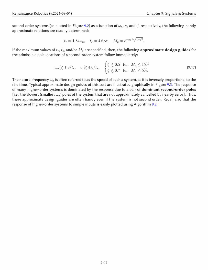
second-order systems (as ploed in Figure 9.2) as a function of ωn, σ, and ζ , respectively, the following handyapproximate relations are readily determined:
tr ≈ 1.8/ωn, ts ≈ 4.6/σ, Mp ≈ e−πζ/√
1−ζ2 .
If the maximum values of tr, ts, and/or Mp are specified, then, the following approximate design guides forthe admissible pole locations of a second-order system follow immediately:
ωn & 1.8/tr, σ & 4.6/ts,
ζ & 0.5 for Mp ≤ 15%
ζ & 0.7 for Mp ≤ 5%.(9.17)
The natural frequency ωn is oen referred to as the speed of such a system, as it is inversely proportional to therise time. Typical approximate design guides of this sort are illustrated graphically in Figure 9.3. The responseof many higher-order systems is dominated by the response due to a pair of dominant second-order poles[i.e., the slowest (smallest ωn) poles of the system that are not approximately cancelled by nearby zeros]. Thus,these approximate design guides are oen handy even if the system is not second order. Recall also that theresponse of higher-order systems to simple inputs is easily ploed using Algorithm 9.2.
9-11

Renaissance Robotics (v.2021-09-01) Chapter 9: Signals & Systems
x
x
θωd
ωn
σ
ℜ(s)
ℑ(s)
Figure 9.1: The poles p± of the system y′′(t) + 2ζωny′(t) + ω2
ny(t) = ω2nu(t) in the complex plane s in terms of
ωn, θ = sin−1 ζ , σ = ζωn, and ωd = ωn√
1− ζ2. The response y(t) to a step input u(t) is ploed in Figure 9.2;note that ωd sets the speed of oscillation and σ sets the exponential rate of decay.
2 4 6 8 10 120
0.2
0.4
0.6
0.8
1
1.2
1.4
tr
t
y(t)
ts
Mp
0 1 2 3 4 5 6 7 8 9 100
0.2
0.4
0.6
0.8
1
1.2
1.4
1.6
1.8
2
p
Figure 9.2: The unit step response of the system y′′(t) + 2ζωny′(t) + ω2
ny(t) = ω2nu(t), for ωn = 1 and (le)
taking ζ = 0.5, with the rise time, seling time, and overshoot indicated, and (right) taking ζ = 0 (dashed),ζ = 0.1, 0.2, 0.3, 0.4, 0.5, 0.6, 0.7, 0.8, and 0.9 (solid), and ζ = 1 (dot-dashed).
−3.5 −3 −2.5 −2 −1.5 −1 −0.5 0 0.5
−1.5
−1
−0.5
0
0.5
1
1.5
1
0.9
0.7 0.5
23
ts
tr
Mp
0.5
0.3 0.1
Figure 9.3: Approximate constraints, or design guides, on the admissible pole locations of a CT second-ordersystem (or a higher-order system whose response is dominated by a pair of second-order poles) in the complexplane s in order to not exceed specified constraints on the rise time, seling time, and overshoot of the system’sstep response (see Figure 9.2), as specified in (9.17).
9-12
Renaissance Robotics (v.2021-09-01) Chapter 9: Signals & Systems
9.3 Z transform methodsThe Z transform (a.k.a. the unilateral Z transform), F (z), of a discrete-time (DT) signal fk for k =0, 1, 2, . . . is defined by
F (z) =∞∑k=0
fkz−k. (9.18a)
Given fk for k = 0, 1, 2, . . ., we define F (z) via (9.18a). The inverse Z transform is given by
fk =1
2πi
∮Γ
F (z)zk−1 dz, (9.18b)
where the complex contour Γ is a circle around the origin in complex plane z that is chosen to be of suicientlysmall radius that it does not contain any singularities9 of F (z) in the complex plane z.
Verification that (9.18b) in fact represents the inverse of the relationship expressed in (9.18a) is straightfor-ward, by substituting (9.18a) into the RHS of (9.18b) and noting (??) and thus that, for a contour Γ given byz = Reiθ for θ = (−π, π) with suiciently small, fixed R (and thus dz = iReiθ dθ), fk is indeed recovered:
1
2πi
∮Γ
[ ∞∑k′=0
fk′z−k′]zk−1 dz =
1
2πi
∫ π
−π
∞∑k′=0
fk′R−k′e−iθk′Rk−1eiθ(k−1)Rieiθ dθ
=∞∑k′=0
fk′Rk−k′
[ 1
2π
∫ π
−πeiθ(k−k′) dθ
]=
∞∑k′=0
fk′Rk−k′δk,k′ = fk,
where the relation (??) has been applied in the second line. The reason that the Rk−k′ factor, for suicientlysmall positive R, is required by this formula is to ensure that the magnitude of the integrand decays to zeroexponentially as k′ →∞, which allows us to swap the order of the integral and the sum using Fubini’s theorem.
As shown below, the forward and inverse transforms expressed by (9.18) are immensely useful when solvingdierence equations (in DT). By (9.18a), knowing fk for k = 0, 1, 2, . . ., one can define F (z) on an appro-priate contour. Conversely, by (9.18b), knowing F (z) on an appropriate contour, one can determine fk fork = 0, 1, 2, . . . As in §9.2, before demonstrating further why such a transformation is useful, we first mentionthat, in practice, you don’t actually need to compute the somewhat involved integrals given in (9.18) in orderto use the Z transform eectively. Rather, it is suicient to reference a table listing some Z transform pairs ina few special cases, as shown in Table 9.1b. Note also the following:
Fact 9.8 The Z transform is linear; that is, superposition holds, and thus if the Z transforms of the sequencesak and bk are A(z) and B(z), then the Z transform of the sequence ck = ak + bk is C(z) = A(z) +B(z).
Fact 9.9 If the Z transform of the sequence fk is F (z), then the Z transform of the scaled sequence gk = bkfkis G(z) =
∑∞k=0 fk(z/b)
−k = F (z/b), and the Z transform of the delayed sequence gk = fk−d is G(z) =∑∞k=0 fk−dz
−k = F (z)/zd.
9.3.1 The Z Transform of translated sequences
Define f [1]k = fk+1 for k = 0, 1, 2, . . .. Then the Z transform of f [1]
k is given by
F [1](z) =∞∑k=0
f[1]k z−k = z
∞∑k=0
fk+1z−(k+1) = z
∞∑k=1
fkz−k = zF (z)− zf0. (9.19)
9That is, the circular contour of integration in the (9.18b) is chosen to be of suiciently small radius that it does not contain anypoints z for which |F (z)| → ∞ as z → z in (9.18a).
9-13

Renaissance Robotics (v.2021-09-01) Chapter 9: Signals & Systems
Similarly, if f [2]k = fk+2 and f [n]
k = fk+n, then
F [2](z) =∞∑k=0
f[2]k z−k = z2F (z)−z2f0−zf1, F [n](z) =
∞∑k=0
f[n]k z−k = znF (z)−znf0−zn−1f1−. . .−zfn−1.
Thus, if f [1]k = fk+1, then F [1](z) = zF (z) − zf0. Conversely, it follows that, if fk+1 = f
[1]k for k = 0, 1, 2, . . .
with f0 = 0, then F (z) = 1zF [1](z). We thus arrive at the most useful interpretation of the z variable:
Fact 9.10 Multiplication of the Z transform of a DT signal by 1/z corresponds to a delay of this signal in the timedomain by one timestep. Similarly, 1/z2 corresponds to a delay of two timesteps, etc.
Defining a new sequence gk = fk+1 − fk for all k and taking the Z transform of gk, applying (9.19), gives
G(z) =∞∑k=0
gkz−k ⇒ [zF (z)− zf0]− F (z) = lim
a→∞
a−1∑k=0
(fk+1 − fk)z−k.
Taking the limit of this expression as z → 1, noting that the limit on the RHS approaches f∞ − f0 if the limitindicated in the above equation is bounded, thus gives
Fact 9.11 (The DT final value theorem) If limk→∞
fk is bounded, then limz→1
(z − 1)F (z) = limk→∞
fk.
On the other hand, it follows directly from the z →∞ limit of (9.18a) that
Fact 9.12 (The DT initial value theorem) limz→∞
F (z) = f0.
9.3.2 Using the Z Transform to solve unforced linear dierence equationsNow consider the unforced linear constant-coeicient second-order dierence equation given by
fk+2 + a1fk+1 + a0fk = 0 with f0, f1 given. (9.20)
Taking the Z transform of this equation and applying the above relations gives∞∑k=0
fk+2 + a1fk+1 + a0fk = 0z−k ⇒ [z2F (z)− z2f0 − zf1] + a1[zF (z)− zf0] + a0[F (z)] = 0
⇒ F (z) =c2z
2 + c1z
z2 + a1z + a0
where c2 = f0, c1 = f1 + a1f0.
Defining p± = (−a1 ±√a2
1 − 4a0)/2 and performing a partial fraction expansion, it follows that
F (z) =c2z
2 + c1z
(z − p+)(z − p−)=
d+z
z − p+
+d−z
z − p−⇒
d+ + d− = c2
−d+p− − d−p+ = c1
⇒
d+ =
c2p+ + c1
p+ − p−d− =
c2p− + c1
p− − p+
.
Thus, by Table 9.1b and the linearity of the Z transform (Fact 9.8), we deduce that
fk = d+pk+ + d−p
k−, (9.21)
thus solving the original dierence equation (9.20). It is seen that, if the magnitudes of p± are less than one,the magnitude of the solution decays with time, whereas if the magnitudes of p± are greater than one, themagnitude of the solution grows with time. A dierence equation of precisely the form given in (9.20) leads tothe well-known Fibonacci’s sequence, as considered in Exercise 9.3.
Higher-order linear dierence equations may be solved in an identical manner, leveraging partial fractionexpansions to split up F (z) into simple terms whose Z transforms may be found in Table 9.1b.
9-14
Renaissance Robotics (v.2021-09-01) Chapter 9: Signals & Systems
9.3.3 Discrete-time (DT) transfer functionsNow consider the forced linear constant-coeicient second-order dierence equation, a.k.a. DT SISO LTI sys-tem, for uk (the output10) given by
uk+2 + a1 uk+1 + a0 uk = b0 ek, (9.22)
where ek (the input) is specified, assuming uk and ek are zero for k < 0. Taking the Z transform now gives
∞∑0
uk+2 + a1 uk+1 + a0 uk = b0 ekz−k ⇒ [z2 + a1 z + a0]U(z) = b0E(z)
⇒ D(z) ,U(z)
E(z)=
b0
z2 + a1 z + a0
=b0
(z − p+)(z − p−), (9.23)
where, again, the poles p± =(− a1 ±
√a2
1 − 4 a0
)/2. The quantity D(z) is known as the transfer function of
the linear system (9.22). Higher-order forced SISO constant-coeicient DT linear systems of the form
uk+n + an−1 uk+n−1 + . . .+ a1 uk+1 + a0 uk = bm ek+m + bm−1 ek+m−1 + . . .+ b1 ek+1 + b0 ek (9.24)
with bm 6= 0 [and, normally, n ≥ m; see §9.3.3.2], may be manipulated in an analogous manner, leading to atransfer function of the form
D(z) =U(z)
E(z)=bm z
m + bm−1 zm−1 + . . .+ b1 z + b0
zn + an−1 zn−1 + . . .+ a1 z + a0
= K(z − z1)(z − z2) · · · (z − zm)
(z − p1)(z − p2) · · · (z − pn). (9.25)
By comparison, the parallels with the CT case in §9.2.3 are clear. Note that, in implementation, it is oen moreconvenient to write (9.24) [in the case that n ≥ m] as
uk = −a1 uk−1 − . . .− an−1 uk−(n−1) − an uk−n + b0ek + b1ek−1 + . . .+ bn−1ek−(n−1) + bnek−n, (9.26)
where, for convenience, we have renumbered the coeicients ak = an−k and bk = bn−k; this form is oenreferred to as a finite impulse response (FIR) filter if ak = 0 for k > 0, and an infinite impulse response(IIR) filter if not. Note that the FIR case is distinguished by an impulse response that vanishes aer finitenumber of steps, whereas [due to the feedback built in to the dierence equation (9.26)] the IIR case is not.
Note that a dierence equation governing a DT system, taken on its own, simply relates linear combinationsof two or more variables describing the system and their tap delays; such an equation does not itself indicateone variable as a “cause” and another as an “eect” in a cause-eect relationship. However, the definition of atransfer function inherently identifies, or defines, a cause-eect or input-output relationship; in the examplesdiscussed above, ek is identified as the input, and uk is identified as the output. This further distinction betweeninput and output is signficant. Almost all systems encountered are causal, meaning that any variable identifiedas an “output” only responds to the current and past “inputs”, but not to future inputs. In the DT seing (incontrast with the CT seing discussed previously), this is facilitated only when m ≤ n in the general higher-order form given above; for further discussion, see §9.3.3.2.
Once a (causal) DT linear system’s transfer function is known, its response to simple inputs is easy tocompute. Noting Table 9.1b, if ek is a unit impulse (that is, ek = δ0,k), then E(z) = 1, and if ek is a unit step[that is, ek = 1 for k ≥ 0], then E(z) = z/(z− 1). In both cases, U(z) is easy to compute from (9.23), and thusuk may be found by partial fraction expansion and subsequent inverse Z transform.
10For the sake of later convenience (in §??), we have changed the leers associated with the inputs and output considered in§9.3.3, where we consider a DT controller D(z) = U(z)/E(z), as compared with §9.2.3, where we considered a CT plant G(s) =Y (s)/U(s).
9-15
Renaissance Robotics (v.2021-09-01) Chapter 9: Signals & Systems
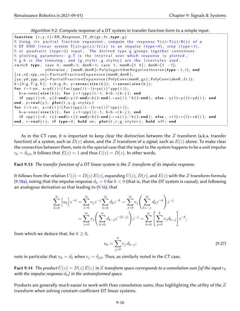
Algorithm 9.2: Compute response of a DT system in transfer function form to a simple input.function [ r , y , t ]= RR_Response_TF_dt ( gz , f z , type , g )% Using i t s p a r t i a l f r a c t i o n expans ion , compute the r e s p o n s e Y ( z )= T ( z ) ∗ R ( z ) o f a% DT SISO l i n e a r system T ( z )= gz ( z ) / f z ( z ) to an impu l se ( type = 0 ) , s t e p ( type = 1 ) ,% or q u a d r a t i c ( type = 2 ) i n p u t . The d e r i v e d type g groups t o g e t h e r c o n v e n i e n t% p l o t t i n g paramete r s : g . T i s the i n t e r v a l o v e r which r e s p o n s e i s p l o t t e d ,% g . h i s the t imes tep , and g . s t y l e r , g . s t y l e y a r e the l i n e s t y l e s used .s w i t c h type , c a s e 0 , numR = 1 ; denR = 1 ; c a s e 1 , numR=[1 0 ] ; denR =[1 −1] ;
o the rw i se , [numR , denR ]= P o l y l o g a r i t h m N e g a t i v e I n v e r s e ( type − 1 , 1 ) ; end[ ra , rd , rpp , rn ]= P a r t i a l F r a c t i o n E x p a n s i o n ( numR , denR ) ;[ ya , yd , ypp , yn ]= P a r t i a l F r a c t i o n E x p a n s i o n ( PolyConv ( numR , gz ) , PolyConv ( denR , f z ) ) ;k = [ 0 : g . T / g . h ] ; t =k ∗ g . h ; y= zeros ( s i z e ( k ) ) ; r = zeros ( s i z e ( k ) ) ;for i = 1 : yn , a=yd ( i ) / ( Fac ( ypp ( i )−1 ) ∗ ya ( i ) ^ ypp ( i ) ) ;
b=a ∗ ones ( s i z e ( k ) ) ; for j = 1 : ypp ( i )−1 , b=b . ∗ ( k−j ) ; endi f ypp ( i ) > 0 , y ( 2 : end )= y ( 2 : end )+ b ( 2 : end ) . ∗ ya ( i ) . ^ k ( 2 : end ) ; else , y ( 1 ) = y ( 1 ) + yd ( i ) ; end
end , y= r e a l ( y ) ; plot ( t , y , g . s t y l e y )for i = 1 : rn , a= rd ( i ) / ( Fac ( rpp ( i )−1 ) ∗ ra ( i ) ^ rpp ( i ) ) ;
b=a ∗ ones ( s i z e ( k ) ) ; for j = 1 : rpp ( i )−1 , b=b . ∗ ( k−j ) ; endi f rpp ( i ) > 0 , r ( 2 : end )= r ( 2 : end )+ b ( 2 : end ) . ∗ ra ( i ) . ^ k ( 2 : end ) ; else , r ( 1 ) = r ( 1 ) + rd ( i ) ; end
end , r = r e a l ( r ) ; i f type > 0 , hold on ; plot ( t , r , g . s t y l e r ) , hold o f f ; end
As in the CT case, it is important to keep clear the distinction between the Z transform (a.k.a. transferfunction) of a system, such as D(z) above, and the Z transform of a signal, such as E(z) above. To make clearthe connection between them, note in the special case that the input to the system happens to be a unit impulseek = δ0,k, it follows that E(z) = 1 and thus U(z) = D(z). In other words,
Fact 9.13 The transfer function of a DT linear system is the Z transform of its impulse response.
It follows from the relation U(z) = D(z)E(z), expanding U(z), D(z), and E(z) with the Z transform formula(9.18a), noting that the impulse response dk = 0 for k < 0 (that is, that the DT system is causal), and followingan analogous derivation as that leading to (9.16), that
∞∑k=0
[uk
]z−k =
∞∑j=0
ejz−j
∞∑k=0
dkz−k =
∞∑j=0
ej
( ∞∑k=−j
dkz−k)z−j
=∞∑j=0
ej
( ∞∑k=0
dk−jz−(k−j)
)z−j =
∞∑k=0
[k∑j=0
ejdk−j
]z−k,
from which we deduce that, for k ≥ 0,
uk =k∑j=0
ej dk−j; (9.27)
note in particular that uk = dk when ej = δj,0. Thus, as similarly noted in the CT case,
Fact 9.14 The product U(z) = D(z)E(z) in Z transform space corresponds to a convolution sum [of the input ekwith the impulse response dk] in the untransformed space.
Products are generally much easier to work with than convolution sums, thus highlighting the utility of the Ztransform when solving constant-coeicient DT linear systems.
9-16

Renaissance Robotics (v.2021-09-01) Chapter 9: Signals & Systems
0 5 10 15 20 25 300
0.2
0.4
0.6
0.8
1
1.2
1.4
1.6
1.8
2
0 10 20 30 40 50 600
0.2
0.4
0.6
0.8
1
1.2
1.4
1.6
1.8
2
Figure 9.4: The unit step response of the system uk+2 + a1uk+1 + a0uk = b0ek, where b0 = 1 + a1 + a0, withr = 0.7 (circles), r = 0.9 (asterisks), and r = 1.0 (squares) for θ = π/5 (le) and θ = π/10 (right), wherer =√a0 and θ = cos−1[−a1/(2r)] (cf. Figure 9.2b). The lines in this figure are drawn to improve readability;
the DT signals are defined only at each step, indicated by the symbols.
9.3.3.1 The transfer function of a DAC – G(s) – ADC cascade
By Fact 9.13, we may determine the transfer function of a DT system, G(z), simply by computing the responseof the system to an impulse input, uk = δ0,k, then taking the Z transform of this response. Applying thisexperiment to a cascade of components given by (i) a digital-to-analog converter (DAC) implementing azero-order-hold11 (ZOH), (ii) a CT system G(s), and (iii) an analog-to-digital converter (ADC) , noting inthis case that u(t) [that is, the input to G(s)] is simply a unit step (with Laplace transform 1/s in CT) followedby a one-timestep-delayed negative unit step, it follows that
G(z) = Z1− e−sh
sG(s)
= (1− z−1)Z
G(s)
s
=z − 1
zZG(s)
s
, (9.28)
where z−1 corresponds to the one-timestep delay, with Laplace transform e−sh, and the shorthand ZG(s)/smeans the Z transform of the discretization of the CT signal whose Laplace transform is G(s)/s. We will makeuse of this convenient (and exact!) expression in Figure ?? and §??.
9.3.3.2 Causal, strictly causal, and noncausal DT systems
We now revisit the dierence equation in (9.24) and its corresponding transfer function in (9.25), where thedegree of the polynomial in the numerator is m, and the degree of the polynomial in the denominator is n.Define the relative degree of such a transfer function as nr = n−m. In DT, systems of this form with nr < 0are, by their very form, noncausal (that is, the output depends, in part, on future values of the input). In §?? wewill further distinguish the DT systems of interest as “plants” G(z) and “controllers” D(z). All real DT plantsG(z), or DT analogs of CT proper (see §9.2.3.1) plants [formed, e.g., via the technique given in (9.28) of §??],are causal, with nr ≥ 0. Further, any controller D(z) must only be based on available measurements, and thusmust also be causal, with nr ≥ 0. If there is significant computation time necessary to compute the control (indigital electronics) before it can be applied back to the system, it is oen most suitable to restrict the controllerto be strictly causal, with nr > 0. Thus, we will focus our aention in this study almost exclusively on the casewith nr ≥ 0; that is, on dierence equations that may be wrien in the form (9.26). Note also that a DT transfer
11That is, holding the value of the analog signal as constant between timesteps
9-17

Renaissance Robotics (v.2021-09-01) Chapter 9: Signals & Systems
function with nr = 0 in (9.24) [that is, with b0 6= 0 in (9.26)], which is causal but not strictly causal, is said tobe semi-causal. Two final catagories of dierence equations are also occasionally encountered: if the outputdepends only on the current and future inputs, the transfer function is said to be anti-causal, and if the outputdepends strictly on future (but not current) inputs, the transfer function is said to be strictly anti-causal.
9-18

Renaissance Robotics (v.2021-09-01) Chapter 9: Signals & Systems
Example 9.2 The step response of second-order DT linear systems
We now focus further on the forced second-order case (9.22), wrien as Y (z) = G(z)U(z), with b0 = 1+a1+a0,when forced by a unit step uk = 1 for k ≥ 0; that is,
G(z) =1 + a1 + a0
z2 + a1z + a0
=1 + a1 + a0
(z − p+)(z − p−)and U(z) =
z
z − 1.
Assuming that the poles are complex, p± =(− a1 ± i
√4a0 − a2
1
)/2 = r e±iθ where
r =√a0 and θ = cos−1
(− a1
2r
),
and have magnitude less than one (i.e., a21/4 < a0 < 1), the solution of this system may again be wrien in
terms of sines and cosines modulated by a decaying exponential: writing the partial fraction expansion
Y (z) = G(z)U(z) =1 + a1 + a0
(z − p+)(z − p−)· z
z − 1=
d+p+
z − p+
+d−p−z − p−
+d0
z − 1,
d+ =
1+a1+a0
(p+−p−)(p+−1),
d− =−(1+a1+a0)
(p+−p−)(p−−1)= d+,
d0 = 1.
and computing the inverse Z transform of Y (z) via Table 9.1b, the closed-form solution of yk for k > 0 is
yk = d+pk+ + d−p
k− + d0 = rk
[dc cos(θ k) + ds sin(θ k)
]+ 1,
dc = d+ + d− = −1,
ds = i(d+ − d−) = − a1+2√4a0−a21
,
as ploed in Figure 9.4. As in the CT case, since the systemG(z) considered in this example is real, the complexpoles p+ and p− come as a conjugate pair. In addition, as consequence of the fact that the input uk to thissystem is also real, the coeicients d+ and d− also work out to be a complex conjugate pair, and thus dc and ds,and yk itself, are real. Again, the speed of oscillation θ and the rate of decay r of this response are a functionof the location of the poles of the transfer function p± = r eiθ. Note also that y0 = y1 = 0; this follows directlyfrom (9.22), noting the k + 2 subscript on y on the LHS and the k subscript on u on the RHS.
As evident in Figure 9.4, rise time tr, seling time ts, and overshoot Mp characterizations, introduced in theCT case in Figure 9.2, may also be defined in the DT case. Appropriate design guides for the pole locations in thez plane in order to ensure specified maximum values of tr, ts, andMp are presented in the following subsection.
9.3.4 Reconciling the Laplace and Z transformsWe now revisit the Laplace transform as defined in (9.7a) and the Z transform as defined in (9.18a):
F (s) =
∫ ∞0
f(t)e−stdt, F (z) =∞∑k=0
fkz−k.
Note that, if we take z = esh where h is the timestep [that is, tk = hk and fk = f(tk)], and if h is small as com-pared with the time scales of the variation of f(t), then F (z), scaled by h, is a rectangular-rule approximationof F (s). Another way of making this connection between the CT analysis and the DT analysis is by comparing
9-19

Renaissance Robotics (v.2021-09-01) Chapter 9: Signals & Systems
−8 −7 −6 −5 −4 −3 −2 −1 0 1−4
−3
−2
−1
0
1
2
3
4
−1 −0.8 −0.6 −0.4 −0.2 0 0.2 0.4 0.6 0.8 1
−1
−0.8
−0.6
−0.4
−0.2
0
0.2
0.4
0.6
0.8
1
Figure 9.5: The mapping of several curves and points between the s plane (le) and the z plane (right) using(9.29). Taking s = a+ bi and z = reiθ, the shaded strip in the s plane with −∞ < a ≤ 0 and −π/h ≤ b ≤ π/hmaps uniquely to the shaded disk in the z plane with r ≤ 1. Points above and below this strip in the s-planedo not map uniquely to points in the z-plane; for example, both points marked by asterisks in the s plane mapto the same point similarly marked in the z plane. This is a manifestation of the aliasing phenomenon depictedin Figure ??.
−1 −0.8 −0.6 −0.4 −0.2 0 0.2 0.4 0.6 0.8 1−1
−0.8
−0.6
−0.4
−0.2
0
0.2
0.4
0.6
0.8
1
0.9
0.8
0.7
0.6
0.5
0.4
0.3
0.2
0.1
π/T
0.9π/T
0.8π/T
0.7π/T
0.6π/T0.5π/T
0.4π/T
0.3π/T
0.2π/T
0.1π/T
π/T
0.9π/T
0.8π/T
0.7π/T
0.6π/T0.5π/T
0.4π/T
0.3π/T
0.2π/T
0.1π/T
Figure 9.6: Approximate constraints, or design guides, on the admissible pole locations of a DT second-ordersystem (or a higher-order system whose response is dominated by a pair of second-order poles) in the complexplane z in order to not exceed specified constraints on the rise time and overshoot of the system’s step response(see Figure 9.4). These DT design guides are found simply by mapping the corresponding CT design guides(see Figure 9.3) using (9.29), and may be drawn with the command zgrid in Matlab syntax. Around thecircumference are marked the values of ωd, from 0.1π/T to π/T , and in the upper-right quadrant are markedthe values of ζ , from 0.1 to 0.9, for the corresponding CT second-order design guides discussed in Example 9.1.
9-20

Renaissance Robotics (v.2021-09-01) Chapter 9: Signals & Systems
the closed-form solutions of the step responses of second-order CT and DT systems, as given in Examples 9.1and 9.2. We see that the laer response is simply a discretization of the former if rk = e−σt and θk = ωdt; thatis, if the CT second-order pole locations s± = −σ± iωd and the DT second-order pole locations z± = re±iθ arerelated such that r = e−σh and θ = ωdh, and thus z± = re±iθ = e(−σ±iωd)h = es±h.
Thus, the pole locations in DT and CT are related by the mapping
z = esh = 1 + sh+s2h2
2!+s3h3
3!+ . . . , (9.29)
as indicated in Figure 9.5. This connection is quite significant. For example, the approximate design guides forCT systems dominated by a pair of second-order poles, as illustrated in Figure 9.3, may be mapped immedi-ately using this relation to obtain corresponding approximate design guides for DT second-order systems, asillustrated in Figure 9.6. It is seen that, for sinusoidal signals (that is, for r = 1), the number of timesteps peroscillation is 2π/θ. It is also seen that the seling time is related to r, with r = 0.9 corresponding to a selingtime of 43 timesteps, r = 0.8 corresponding to a seling time of 21 timesteps, and r = 0.6 corresponding to aseling time of 9 timesteps.
For small h, (9.29) provides a simple connection between s-plane pole locations in the vicinity of s = 0 andthe (scaled) z-plane pole locations in the vicinity of z = 1 via Euler’s approximation
z ≈ 1 + sh. (9.30)
That is, for small h, the neighborhood of z = 1 in the z plane may be interpreted in a similar fashion as the(scaled) neighborhood of s = 0 in the s plane, and the three families of design guides (for tr, ts, and Mp) inthese two regions indeed look quite similar.
9.3.4.1 Tustin’s approximation
For larger h, Euler’s approximation is not accurate. Motivated by the accuracy analysis of the CN method givenin §??, the following rational approximation of (9.29), referred to in this seing as Tustin’s approximation, ispreferred for most applications:
z ≈ 1 + sh/2
1− sh/2 = 1 + sh+s2h2
2+s3h3
4+ . . . ⇔ s ≈ 2
h
z − 1
z + 1. (9.31)
Conveniently, both the exact mapping (9.29) and Tustin’s approximation (9.31) map the le half plane of s tothe interior of the unit circle in z; in particular, the stability boundary of s (the imaginary axis) maps to thestability boundary of z (the unit circle). This is why Tustin’s approximation is strongly preferred over Euler’sapproximation (9.30), or other manners of truncating or approximating (9.29).
To see how to use Tustin’s rule to approximate a general CT dierential equation [interpreted in §?? as acontroller] whose Laplace transform is D(s) with a DT dierence equation whose Z transform is D(z), it isuseful to consider first the transfer function of the following simple dierential equation, with u(t) and e(t)taken to be zero for t < 0:
U(s)
E(s)= D(s) =
s+ a
s+ p⇒ (s+ p)U(s) = (s+ a)E(s) ⇒ du
dt+ pu =
de
dt+ ae.
Approximating the time derivatives in this ODE with the CN method (see §8), we may write
uk − uk−1
h+ p
uk + uk−1
2=ek − ek−1
h+ a
ek + ek−1
2.
Taking the Z transform of this dierence equation and rearranging leads immediately to
9-21
Renaissance Robotics (v.2021-09-01) Chapter 9: Signals & Systems
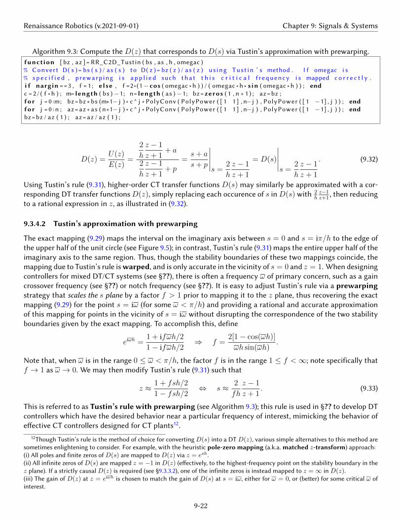
Algorithm 9.3: Compute the D(z) that corresponds to D(s) via Tustin’s approximation with prewarping.function [ bz , az ]= RR_C2D_Tustin ( bs , as , h , omegac )% Convert D( s )= bs ( s ) / as ( s ) to D( z )= bz ( z ) / as ( z ) u s i n g Tus t in ’ s method . I f omegac i s% s p e c i f i e d , p rewarp ing i s a p p l i e d such t h a t t h i s c r i t i c a l f r e q u e n c y i s mapped c o r r e c t l y .i f nargin ==3 , f = 1 ; else , f =2∗ (1− cos ( omegac ∗h ) ) / ( omegac ∗h ∗ s in ( omegac ∗h ) ) ; endc = 2 / ( f ∗h ) ; m= length ( bs )−1 ; n= length ( as )−1 ; bz = zeros ( 1 , n + 1 ) ; az = bz ;for j = 0 :m; bz = bz + bs (m+1− j ) ∗ c ^ j ∗ PolyConv ( PolyPower ( [ 1 1 ] , n−j ) , PolyPower ( [ 1 −1] , j ) ) ; endfor j = 0 : n ; az = az + as ( n+1− j ) ∗ c ^ j ∗ PolyConv ( PolyPower ( [ 1 1 ] , n−j ) , PolyPower ( [ 1 −1] , j ) ) ; endbz = bz / az ( 1 ) ; az = az / az ( 1 ) ;
D(z) =U(z)
E(z)=
2
h
z − 1
z + 1+ a
2
h
z − 1
z + 1+ p
=s+ a
s+ p
∣∣∣∣∣s =
2
h
z − 1
z + 1
= D(s)
∣∣∣∣∣s =
2
h
z − 1
z + 1
. (9.32)
Using Tustin’s rule (9.31), higher-order CT transfer functions D(s) may similarly be approximated with a cor-responding DT transfer functions D(z), simply replacing each occurence of s in D(s) with 2
hz−1z+1
, then reducingto a rational expression in z, as illustrated in (9.32).
9.3.4.2 Tustin’s approximation with prewarping
The exact mapping (9.29) maps the interval on the imaginary axis between s = 0 and s = iπ/h to the edge ofthe upper half of the unit circle (see Figure 9.5); in contrast, Tustin’s rule (9.31) maps the entire upper half of theimaginary axis to the same region. Thus, though the stability boundaries of these two mappings coincide, themapping due to Tustin’s rule is warped, and is only accurate in the vicinity of s = 0 and z = 1. When designingcontrollers for mixed DT/CT systems (see §??), there is oen a frequency ω of primary concern, such as a gaincrossover frequency (see §??) or notch frequency (see §??). It is easy to adjust Tustin’s rule via a prewarpingstrategy that scales the s plane by a factor f > 1 prior to mapping it to the z plane, thus recovering the exactmapping (9.29) for the point s = iω (for some ω < π/h) and providing a rational and accurate approximationof this mapping for points in the vicinity of s = iω without disrupting the correspondence of the two stabilityboundaries given by the exact mapping. To accomplish this, define
eiωh =1 + ifωh/21− ifωh/2
⇒ f =2[1− cos(ωh)]
ωh sin(ωh).
Note that, when ω is in the range 0 ≤ ω < π/h, the factor f is in the range 1 ≤ f <∞; note specifically thatf → 1 as ω → 0. We may then modify Tustin’s rule (9.31) such that
z ≈ 1 + fsh/2
1− fsh/2 ⇔ s ≈ 2
fh
z − 1
z + 1. (9.33)
This is referred to as Tustin’s rule with prewarping (see Algorithm 9.3); this rule is used in §?? to develop DTcontrollers which have the desired behavior near a particular frequency of interest, mimicking the behavior ofeective CT controllers designed for CT plants12.
12Though Tustin’s rule is the method of choice for converting D(s) into a DT D(z), various simple alternatives to this method aresometimes enlightening to consider. For example, with the heuristic pole-zero mapping (a.k.a. matched z-transform) approach:(i) All poles and finite zeros of D(s) are mapped to D(z) via z = esh.(ii) All infinite zeros of D(s) are mapped z = −1 in D(z) (eectively, to the highest-frequency point on the stability boundary in thez plane). If a strictly causal D(z) is required (see §9.3.3.2), one of the infinite zeros is instead mapped to z =∞ in D(z).(iii) The gain of D(z) at z = eiωh is chosen to match the gain of D(s) at s = iω, either for ω = 0, or (beer) for some critical ω ofinterest.
9-22
Renaissance Robotics (v.2021-09-01) Chapter 9: Signals & Systems
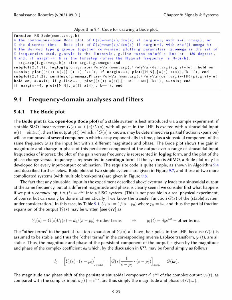
Algorithm 9.4: Code for drawing a Bode plot.function RR_Bode ( num , den , g , h )% The cont inuous−t ime Bode p l o t o f G( s )=num ( s ) / den ( s ) i f n a r g i n =3 , with s = ( i omega ) , o r% the d i s c r e t e−t ime Bode p l o t o f G( z )=num ( z ) / den ( z ) i f n a r g i n =4 , with z =e ^ ( i omega h ) .% The d e r i v e d type g groups t o g e t h e r c o n v e n i e n t p l o t t i n g paramete r s : g . omega i s the s e t o f% f r e q u e n c i e s used , g . s t y l e i s the l i n e s t y l e , g . l i n e t u r n s on / o f f a l i n e a t −180 degrees ,% and , i f n a r g i n =4 , h i s the t i m e s t e p ( where the Nyquis t f r e q u e n c y i s N= p i / h ) .
a rg =exp ( i ∗ g . omega ∗h ) ; e l s e arg = i ∗ g . omega ; endsubplot ( 2 , 1 , 1 ) , loglog ( g . omega , abs ( P o l y V a l ( num , arg ) . / P o l y V a l ( den , arg ) ) , g . s t y l e ) , hold ona= axis ; plot ( [ a ( 1 ) a ( 2 ) ] , [ 1 1 ] , ’ k : ’ ) , i f nargin ==4 , plot ( [N N] , [ a ( 3 ) a ( 4 ) ] , ’ k−− ’ ) , endsubplot ( 2 , 1 , 2 ) , semilogx ( g . omega , Phase ( P o l y V a l ( num , arg ) . / P o l y V a l ( den , arg ) ) ∗ 1 8 0 / pi , g . s t y l e )hold on , a= axis ; i f g . l i n e ==1 , plot ( [ a ( 1 ) a ( 2 ) ] , [ − 1 8 0 −180] , ’ k : ’ ) , a= axis ; endi f nargin ==4 , plot ( [N N] , [ a ( 3 ) a ( 4 ) ] , ’ k−− ’ ) , end
9.4 Frequency-domain analyses and filters
9.4.1 The Bode plot
The Bode plot (a.k.a. open-loop Bode plot) of a stable system is best introduced via a simple experiment: ifa stable SISO linear system G(s) = Y (s)/U(s), with all poles in the LHP, is excited with a sinusoidal inputu(t) = sin(ωt), then the output y(t) (which, ifG(s) is known, may be determined via partial fraction expansion)will be composed of several components which decay exponentially in time, plus a sinusoidal component of thesame frequency ω as the input but with a dierent magnitude and phase. The Bode plot shows the gain inmagnitude and change in phase of this persistent component of the output over a range of sinusoidal inputfrequencies of interest; the plot of the gain versus frequency is represented in loglog form, and the plot of thephase change versus frequency is represented in semilogx form. If the system is MIMO, a Bode plot may bedeveloped for every input/output combination. The requisite code is quite simple, as shown in Algorithm 9.4and described further below. Bode plots of two simple systems are given in Figure 9.7, and those of two morecomplicated systems (with multiple breakpoints) are given in Figure 9.8.
The fact that any sinusoidal input in the experiment described above eventually leads to a sinusoidal outputat the same frequency, but at a dierent magnitude and phase, is clearly seen if we consider first what happensif we put a complex input u1(t) = eiωt into a SISO system. [This is not possible in a real physical experiment,of course, but can easily be done mathematically if we know the transfer function G(s) of the (stable) systemunder consideration.] In this case, by Table 9.1, U1(s) = 1/(s− p0) where p0 = iω, and thus the partial fractionexpansion of the output Y1(s) may be wrien [see §??] as
Y1(s) = G(s)U1(s) = d0/(s− p0) + other terms ⇒ y1(t) = d0eiωt + other terms.
The “other terms” in the partial fraction expansion of Y1(s) all have their poles in the LHP, because G(s) isassumed to be stable, and thus the “other terms” in the corresponding inverse Laplace transform, y1(t), are allstable. Thus, the magnitude and phase of the persistent component of the output is given by the magnitudeand phase of the complex coeicient d0 which, by the discussion in §??, may be found simply as follows:
d0 =[Y1(s) · (s− p0)
]s=iω
=[G(s)
1
s− p0
· (s− p0)]s=iω
= G(iω).
The magnitude and phase shi of the persistent sinusoidal component d0eiωt of the complex output y1(t), as
compared with the complex input u1(t) = eiωt, are thus simply the magnitude and phase of G(iω).
9-23

Renaissance Robotics (v.2021-09-01) Chapter 9: Signals & Systems
Consider next what happens if we put the complex input u2(t) = e−iωt into the system:
U2(s) = 1/(s+ p0) where p0 = iω, Y2(s) = G(s)U2(s) = c0/(s+ p0) + other terms ⇒
y2(t) = c0e−iωt + other terms, c0 =
[Y2(s) · (s+ p0)
]s=−iω
=[G(s)
1
s+ p0
· (s+ p0)]s=−iω
= G(iω).
The magnitude and phase shi of the persistent sinusoidal component c0e−iωt of the complex output y2(t), as
compared with the complex input u2(t) = e−iωt, are thus simply the magnitude of G(iω) and the phase ofG(iω), which equals the negative of the phase of G(iω).
Finally, consider what happens if we put the real input u3(t) = [u1(t) +u2(t)]/2 = cos(ωt) into the system.Appealing to superposition and noting that a sin(x) + b cos(x) =
√a2 + b2 sin(x+ ψ) where ψ = atan2(b, a),
y3(t) = [y1(t) + y2(t)]/2 = (d0eiωt + c0e
−iωt)/2 + other terms
= G(iω)[cos(ωt) + i sin(ωt)] +G(iω)[cos(ωt)− i sin(ωt)]/2 + other terms
= [G(iω) +G(iω)] cos(ωt)/2 + [G(iω)−G(iω)]i sin(ωt)/2 + other terms= <G(iω) cos(ωt)−=G(iω) sin(ωt) + other terms= |G(iω)| sin[ωt+ atan2(<G(iω),−=G(iω))] + other terms
= |G(iω)| sin[ωt+π
2+ ∠G(iω)] + other terms = |G(iω)| cos[ωt+ ∠G(iω)] + other terms. (9.34)
The magnitude a and phase shi φ of the persistent sinusoidal component a cos(ωt + φ) of the real outputy3(t), as compared with the real input u3(t) = cos(ωt), are thus, again, simply the magnitude and phase ofG(iω). An alternative derivation that leads to the same result is considered in Exercise 9.8.
Computing the Bode plot of DT systems
By (9.29), a Bode plot in DT may be drawn with the same code as that used in CT, taking z = eiωh rather thans = iω when evaluating the response of the transfer function at various frequencies. Note that the frequencyresponse of a DT system is only defined up to the Nyquist frequency, and thus a Bode plot in DT should onlybe drawn up to the Nyquist frequency.
Computing the Bode plot of unstable systems†
A Bode plot may also be developed for unstable systems. If the transfer function G(s) of an unstable systemis known, the process of computing its Bode plot is identical to that described above: simply calculate themagnitude and phase of G(iω) for the relevant range of values of ω. Note that it doesn’t maer that some ofthe components of the partial fraction expansion of Y (s) have RHP poles in this case, because we need notactually perform the experiment described above, and thus we need not even consider y(t).
If the transfer functionG(s) of an unstable system is not known, however, the computation described abovecan not be performed, and the experiment described in the first paragraph of §9.4.1 would be inconclusive, asthe response would be dominated by one or more exponentially-growing component(s). However, if we canguess a simple D(s) such that the closed-loop transfer function H(s) = G(s)D(s)/[1 + G(s)D(s)] is stable(see Figure ?? and the introduction to §11), then the Bode plot ofH(s) may be determined experimentally13 and,sinceD(s) is known, the magnitude and phase ofG(iω) for the corresponding range of ω may thus be deduced.Practically, it is oen possible to guess a stabilizing controller for an unmodelled unstable system G(s) that isadequate to determine its Bode plot; for example, ifD(s) = K stabilizes the closed-loop system for some value
13As described in the first paragraph of §9.4.1; again, see Figure ?? and the introduction to §11.
9-24
Renaissance Robotics (v.2021-09-01) Chapter 9: Signals & Systems
10 10 10
10−1
100
−1 0 1−100
−80
−60
−40
−20
0
slope = −1
10−2
10−1
100
101
10−1
100
101
−150
−100
−50
0
slope = −2
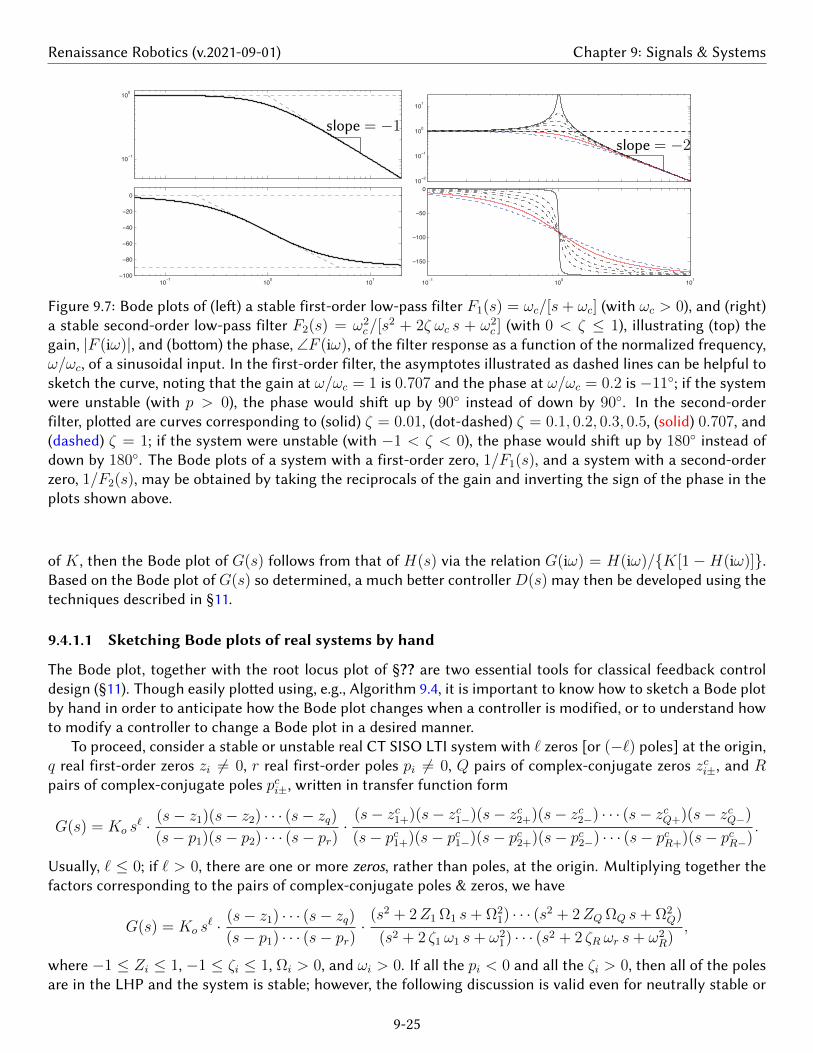
Figure 9.7: Bode plots of (le) a stable first-order low-pass filter F1(s) = ωc/[s+ ωc] (with ωc > 0), and (right)a stable second-order low-pass filter F2(s) = ω2
c/[s2 + 2ζ ωc s + ω2
c ] (with 0 < ζ ≤ 1), illustrating (top) thegain, |F (iω)|, and (boom) the phase, ∠F (iω), of the filter response as a function of the normalized frequency,ω/ωc, of a sinusoidal input. In the first-order filter, the asymptotes illustrated as dashed lines can be helpful tosketch the curve, noting that the gain at ω/ωc = 1 is 0.707 and the phase at ω/ωc = 0.2 is −11; if the systemwere unstable (with p > 0), the phase would shi up by 90 instead of down by 90. In the second-orderfilter, ploed are curves corresponding to (solid) ζ = 0.01, (dot-dashed) ζ = 0.1, 0.2, 0.3, 0.5, (solid) 0.707, and(dashed) ζ = 1; if the system were unstable (with −1 < ζ < 0), the phase would shi up by 180 instead ofdown by 180. The Bode plots of a system with a first-order zero, 1/F1(s), and a system with a second-orderzero, 1/F2(s), may be obtained by taking the reciprocals of the gain and inverting the sign of the phase in theplots shown above.
of K , then the Bode plot of G(s) follows from that of H(s) via the relation G(iω) = H(iω)/K[1 −H(iω)].Based on the Bode plot of G(s) so determined, a much beer controller D(s) may then be developed using thetechniques described in §11.
9.4.1.1 Sketching Bode plots of real systems by hand
The Bode plot, together with the root locus plot of §?? are two essential tools for classical feedback controldesign (§11). Though easily ploed using, e.g., Algorithm 9.4, it is important to know how to sketch a Bode plotby hand in order to anticipate how the Bode plot changes when a controller is modified, or to understand howto modify a controller to change a Bode plot in a desired manner.
To proceed, consider a stable or unstable real CT SISO LTI system with ` zeros [or (−`) poles] at the origin,q real first-order zeros zi 6= 0, r real first-order poles pi 6= 0, Q pairs of complex-conjugate zeros zci±, and Rpairs of complex-conjugate poles pci±, wrien in transfer function form
G(s) = Ko s` · (s− z1)(s− z2) · · · (s− zq)
(s− p1)(s− p2) · · · (s− pr)· (s− zc1+)(s− zc1−)(s− zc2+)(s− zc2−) · · · (s− zcQ+)(s− zcQ−)
(s− pc1+)(s− pc1−)(s− pc2+)(s− pc2−) · · · (s− pcR+)(s− pcR−).
Usually, ` ≤ 0; if ` > 0, there are one or more zeros, rather than poles, at the origin. Multiplying together thefactors corresponding to the pairs of complex-conjugate poles & zeros, we have
G(s) = Ko s` · (s− z1) · · · (s− zq)
(s− p1) · · · (s− pr)· (s2 + 2Z1 Ω1 s+ Ω2
1) · · · (s2 + 2ZQ ΩQ s+ Ω2Q)
(s2 + 2 ζ1 ω1 s+ ω21) · · · (s2 + 2 ζR ωr s+ ω2
R),
where −1 ≤ Zi ≤ 1, −1 ≤ ζi ≤ 1, Ωi > 0, and ωi > 0. If all the pi < 0 and all the ζi > 0, then all of the polesare in the LHP and the system is stable; however, the following discussion is valid even for neutrally stable or
9-25
Renaissance Robotics (v.2021-09-01) Chapter 9: Signals & Systems
unstable systems. Evaluating at s = iω gives
G(iω) = Ko(iω)` · (iω − z1) · · · (iω − zq)(iω − p1) · · · (iω − pr)
· (−ω2 + 2Z1 Ω1 iω + Ω21) · · · (−ω2 + 2ZQ ΩQ iω + Ω2
Q)
(−ω2 + 2 ζ1 ω1 iω + ω21) · · · (−ω2 + 2 ζR ωR iω + ω2
R), (9.35)
Noting that G(iω) above is the product of three types of terms, the Bode plot may be sketched using thefollowing handy rules14 (Bode 1930):
1. For small ω, the gain and phase of the Bode plot approach the gain and phase of the following expression:
G(iω) ≈ (iω)`Ko[(−z1) (−z2) · · · (−zq) · Ω21 Ω2
2 · · ·Ω2Q]/[(−p1) (−p2) · · · (−pr) · ω2
1 ω22 · · ·ω2
R].
2. The frequencies |z1|, . . . , |zq|; |p1|, . . . , |pr|; Ω1, . . . ,ΩQ;ω1, . . . , ωR are referred to as breakpoints. Start-ing from the asymptote at the far le of the gain and phase plots and working from le to right, the gain andphase components of the Bode plot change in an orderly fashion in the vicinity of each breakpoint:
2a. In the vicinity of each first-order pole [resp., zero] of multiplicity k, the slope of the gain curve decreases[resp., increases] by k. In the vicinity of each LHP first-order pole [resp., zero] of multiplicity k, the phasedecreases [resp., increases] by k · 90; in the vicinity of each RHP first-order pole [resp., zero] of multiplicity k,the phase increases [resp., decreases] by k · 90. The slope of the gain curve and the value of the phase curvechange gradually over a range of frequencies stretching from one order of magnitude below to one order ofmagnitude above the breakpoint, as illustrated in Figure 9.7a.
2b. In the vicinity of each pair of complex-conjugate poles [resp., zeros] of multiplicity k, the slope of the gaincurve decreases [resp., increases] by 2 k. In the vicinity of each pair of LHP complex-conjugate poles [resp.,zeros] of multiplicity k, the phase decreases [resp., increases] by k · 180; in the vicinity of each pair of RHPcomplex-conjugate poles [resp., zeros] of multiplicity k, the phase increases [resp., decreases] by k · 180. Theslope of the gain curve and the value of the phase curve change gradually over a range of frequencies stretchingfrom one order of magnitude below to one order of magnitude above the breakpoint, as illustrated in Figure9.7b. The precise behavior of both curves in the vicinity of the breakpoint depends on the damping ζi [resp.,Zi], with small values of |ζi| [resp., |Zi|] resulting in a resonance [resp., anti-resonance]; that is, a responsewith large [resp., small] gain in the immediate vicinity of the breakpoint.
When sketching a Bode plot, it is useful to ignore, at first, the fact that the slope of the gain curve and thevalue of the phase curve change gradually over two decades around the breakpoints, and simply plot straight-line asymptotes between each breakpoint. With these asymptotes as guides, the gain and phase curves maythen be sketched by rounding out the corners of these asymptotes, using Figures 9.7a and b as guides.
Drawing the asymptotes between the breakpoints of a Bode plot, using rules 2a and 2b above while workingfrom low frequencies to high frequencies, is in fact quite straightforward. The slope j of the asymptotes for anygiven ω between the breakpoints in the system G(iω) in (9.35) may be computed simply by assuming (even ifits not true) that ω is much smaller than the higher-frequency breakpoints and that ω is much larger than thelower-frequency breakpoints, thus allowing each first-order and second-order factor in both the numerator anddenominator of (9.35) to be reduced to either its first or last term as appropriate; the slope j is then given simplyby the remaining power of ω in the numerator minus the remaining power of ω in the denominator. Further,in systems that are both stable (with no RHP poles) and minimum phase (with no RHP zeros; see §??), thecorresponding phase is simply j · 90 (mod 360); this useful rule of thumb is referred to as Bode’s gain/phaserelationship.
14Many texts cite the gain in terms of decibels (dB), defined as 20 · log10 of the value. We avoid this convention, so that integerslopes of the gain curve on log-log plots are more readily recognized. If a gain in decibels is used, all slopes are multiplied by a factorof 20.
9-26
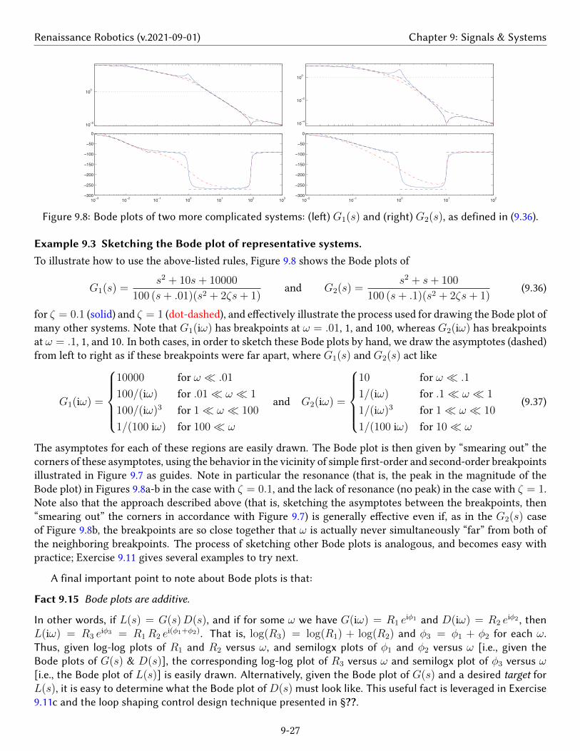
Renaissance Robotics (v.2021-09-01) Chapter 9: Signals & Systems
10−5
100
10−3
10−2
10−1
100
101
102
103
−300
−250
−200
−150
−100
−50
0
10−4
10−2
100
10−2
10−1
100
101
102
−300
−250
−200
−150
−100
−50
0
Figure 9.8: Bode plots of two more complicated systems: (le) G1(s) and (right) G2(s), as defined in (9.36).
Example 9.3 Sketching the Bode plot of representative systems.To illustrate how to use the above-listed rules, Figure 9.8 shows the Bode plots of
G1(s) =s2 + 10s+ 10000
100 (s+ .01)(s2 + 2ζs+ 1)and G2(s) =
s2 + s+ 100
100 (s+ .1)(s2 + 2ζs+ 1)(9.36)
for ζ = 0.1 (solid) and ζ = 1 (dot-dashed), and eectively illustrate the process used for drawing the Bode plot ofmany other systems. Note that G1(iω) has breakpoints at ω = .01, 1, and 100, whereas G2(iω) has breakpointsat ω = .1, 1, and 10. In both cases, in order to sketch these Bode plots by hand, we draw the asymptotes (dashed)from left to right as if these breakpoints were far apart, where G1(s) and G2(s) act like
G1(iω) =
10000 for ω .01
100/(iω) for .01 ω 1
100/(iω)3 for 1 ω 100
1/(100 iω) for 100 ω
and G2(iω) =
10 for ω .1
1/(iω) for .1 ω 1
1/(iω)3 for 1 ω 10
1/(100 iω) for 10 ω
(9.37)
The asymptotes for each of these regions are easily drawn. The Bode plot is then given by “smearing out” thecorners of these asymptotes, using the behavior in the vicinity of simple rst-order and second-order breakpointsillustrated in Figure 9.7 as guides. Note in particular the resonance (that is, the peak in the magnitude of theBode plot) in Figures 9.8a-b in the case with ζ = 0.1, and the lack of resonance (no peak) in the case with ζ = 1.Note also that the approach described above (that is, sketching the asymptotes between the breakpoints, then“smearing out” the corners in accordance with Figure 9.7) is generally eective even if, as in the G2(s) caseof Figure 9.8b, the breakpoints are so close together that ω is actually never simultaneously “far” from both ofthe neighboring breakpoints. The process of sketching other Bode plots is analogous, and becomes easy withpractice; Exercise 9.11 gives several examples to try next.
A final important point to note about Bode plots is that:
Fact 9.15 Bode plots are additive.
In other words, if L(s) = G(s)D(s), and if for some ω we have G(iω) = R1 eiφ1 and D(iω) = R2 e
iφ2 , thenL(iω) = R3 e
iφ3 = R1R2 ei(φ1+φ2). That is, log(R3) = log(R1) + log(R2) and φ3 = φ1 + φ2 for each ω.
Thus, given log-log plots of R1 and R2 versus ω, and semilogx plots of φ1 and φ2 versus ω [i.e., given theBode plots of G(s) & D(s)], the corresponding log-log plot of R3 versus ω and semilogx plot of φ3 versus ω[i.e., the Bode plot of L(s)] is easily drawn. Alternatively, given the Bode plot of G(s) and a desired target forL(s), it is easy to determine what the Bode plot of D(s) must look like. This useful fact is leveraged in Exercise9.11c and the loop shaping control design technique presented in §??.
9-27

Renaissance Robotics (v.2021-09-01) Chapter 9: Signals & Systems
Algorithm 9.5: Code for computing n’th-order Buerworth filters with cuto frequency ωc = 1.function [num , den ]= R R _ B u t t e r w o r t h _ F i l t e r ( n )p=exp ( i ∗ pi ∗ ( 2 ∗ [ 1 : n]−1+n ) / ( 2 ∗ n ) ) ; num = 1 ; den= Po ly ( p ) ;
9.4.2 Low-pass, high-pass, band-pass, and band-stop filtersWe now explore the concept of rational CT filters; that is, of tunable systems (usually implemented as electriccircuits, as discussed in §10) which selectively “accept” and “reject” the various frequency components of asignal. The goal an ideal filter is to have a gain of 1 and a phase of 0 over a specified passband of frequencies,and a gain of nearly 0 over the remaining frequencies (referred to as the stopband). Unfortunately, no rationalfilters ever aain this ideal; this section discusses a few of the common families of filters available which aemptto approximate this ideal behavior.
An ideal low-pass filter has a passband of all frequencies below a cuto frequency ωc, and a stopbandof all frequencies above this cuto frequency. The simplest realizable low-pass filters are the first-order filterF1(s) = 1/[1 + (s/ωc)] depicted in Figure 9.7a and the second-order filter F2(s) = 1/[1 + 2ζ(s/ωc) + (s/ωc)
2]depicted in Figure 9.7b (generally, ζ = 0.707 is a good choice). For both filters, the gain approaches 1 andthe phase approaches 0 for frequencies ω much smaller than ωc, and the gain rolls o (on a log-log plot, ata slope of −1 in the first-order case and a slope of −2 in the second-order case) for frequencies much largerthan ωc. Neither filter has the ideal sharp cuto at the boundary between the passband and the stopband asdescribed above; the higher-order filters discussed below provide a variety of ways of achieving a sharper cutoat the boundary between the passband and the stopband, at the cost of sometimes significant phase loss, even atfrequencies down to an order of magnitude below the cuto frequency15.
Note that an ideal high-pass filter is a filter with a passband of all frequencies above the cuto frequencyωc, and a stopband of all frequencies below the cuto frequency. Any realizable low-pass filter may be convertedinto a high pass filter simply by replacing (s/ωc) with (ωc/s) in its transfer function and simplifying; we thus focusexclusively on low-pass filter design in the discussion that follows.
Note also that an ideal band-pass filter is a filter with a passband of all frequencies between two criticalfrequencies, and a stopband at all other frequencies, whereas an ideal band-stop filter is a filter with a stop-band of all frequencies between two critical frequencies, and a passband at all other frequencies. A band-passfilter may be constructed from a low-pass filter and a high-pass filter connected in series, whereas a band-stop filtermay be constructed from a low-pass filter and a high-pass filter connected in parallel.
9.4.2.1 Maximal flatness filters: Buerworth and Bessel
Recalling Figure ??b and defining rk for k = 1, . . . , 2n as the (2n)’th roots of −1, a Buerworth filter isdefined by a transfer function with poles given by those values of pk , (irk) which have a negative real part:
FBun (s) =
1
Bn(s)where s = s/ωc, Bn(x) =
n∏k=1
(x− pk), and pk = eiπ(2k−1+n)/(2n). (9.38)
Noting that the complex poles come in complex-conjugate pairs, Bn(x) may be wrien with real coeicientsby grouping together those factors in the above expression with complex-conjugate poles, such as p1 and pn;
15Such phase loss can have important negative consequences; as discussed in §??, loss of phase at crossover can lead to a significantloss of closed-loop system performance, and even closed-loop instability. Thus, if a low-pass filter is used to reject high-frequencymeasurement noise in a feedback control loop, the cuto frequency of the low-pass filter should be placed at least an order ofmagnitude above the crossover frequency of the closed-loop system.
9-28
Renaissance Robotics (v.2021-09-01) Chapter 9: Signals & Systems
Algorithm 9.6: Code for computing n’th-order Bessel filters with cuto frequency ωc = 1.function [num , den ]= R R _ B e s s e l _ F i l t e r ( n )k =[ n : − 1 : 0 ] ; den= Fac ( 2 ∗ n−k ) . / Fac ( n−k ) . / Fac ( k ) . / 2 . ^ ( n−k ) ; num= P o l y V a l ( den , 0 ) ;
the first eight of the resulting normalized Buerworth polynomials Bn(x) are:
B1(x) = (x+ 1),
B2(x) = (x2 + 1.41421x+ 1),
B3(x) = (x+ 1)(x2 + x+ 1),
B4(x) = (x2 + 0.76537x+ 1)(x2 + 1.84776x+ 1),
B5(x) = (x+ 1)(x2 + 0.61803x+ 1)(x2 + 1.61803x+ 1),
B6(x) = (x2 + 0.51764x+ 1)(x2 + 1.41421x+ 1)(x2 + 1.93185x+ 1),
B7(x) = (x+ 1)(x2 + 0.44504x+ 1)(x2 + 1.24698x+ 1)(x2 + 1.80194x+ 1),
B8(x) = (x2 + 0.39018x+ 1)(x2 + 1.11114x+ 1)(x2 + 1.66294x+ 1)(x2 + 1.96157x+ 1).
Bode plots of the first 6 Buerworth filters are given in Figure 9.9a. For sinusoidal inputs at normalized fre-quency ω = ω/ωc, the gain of the n’th-order Buerworth filter is given by the square root of
|FBun (iω)|2 = FBu
n (iω)Fn(−iω) =1∏n
k=1[(iω)− pk]∏n
k=1[(−iω)− pk]=
1
ω2n + 1,
where the expression on the right follows simply because ip1, . . . , ipn,−ip1, . . . ,−ipn is the set of all roots ofthe equation ω2n + 1 = 0. Defining the gain GBu
n (ω) = 1/(ω2n + 1)1/2, it follows that
dGBun (ω)
dω= −n [GBu
n (ω)]3 ω2n−1 < 0 and GBun (ω) = 1− 1
2ω2n +
3
8ω4n + . . . ; (9.39)
that is,GBun (ω) decreases monotonically with ω and the first (2n−1) derivatives ofGBu
n (ω) evaluated at ω = 0are zero; this property is referred to as maximal flatness of the gain curve, and is the central strength of theBuerworth filter. Unfortunately, as seen in Figure 9.9a, the higher-order Buerworth filters with sharp rollofor ω > 1 suer from significant phase loss over a large range of frequencies below ωc.
Note that a Linkwitz-Riley (L-R) filter is simply two Buerworth filters applied in series. Linkwitz-Rileyfilters are particularly convenient in audio crossovers, as the magnitudes of a low-pass L-R filter (routed to awoofer) and a high-pass L-R filter (routed to a tweeter) add to unity across all frequencies16.
A Bessel filter is defined by the transfer function
FBen (s) =
θn(0)
θn(s)where s = s/ωc and θn(x) =
n∑k=0
(2n− k)!
(n− k)! k!
xk
2n−k; (9.40)
16Midrange speakers may also be added to an audio system using multiple matched pairs of low-pass/high-pass L-R filters.
9-29

Renaissance Robotics (v.2021-09-01) Chapter 9: Signals & Systems
10−6
10−4
10−2
100
10−1
100
101
−500
−400
−300
−200
−100
0
10−8
10−6
10−4
10−2
100
10−1
100
101
102
−500
−400
−300
−200
−100
0
Figure 9.9: Bode plots of (solid) first-order to (dashed) sixth-order (le) Buerworth filters and (right) Besselfilters, illustrating (top) the magnitude, |G(iω)|, and (boom) the phase, ∠G(iω), of the system response as afunction of the normalized frequency, ω = ω/ωc, of a sinusoidal input. In the vicinity of ωc, the Buerworthfilter is optimal in terms of the flatness of the gain, whereas the Bessel filter is optimal in terms of the flatnessof the group delay (that is, the phase). Note that the slope of the magnitude plot of the n’th-order filter in bothcases is monotonic, and approaches −n for ω 1.
the θn(x) functions are known as reverse Bessel polynomials, the first eight of which are given by
θ1(x) = x+ 1,
θ2(x) = x2 + 3x+ 3,
θ3(x) = x3 + 6x2 + 15x+ 15,
θ4(x) = x4 + 10x3 + 45x2 + 105x+ 105,
θ5(x) = x5 + 15x4 + 105x3 + 420x2 + 945x+ 945,
θ6(x) = x6 + 21x5 + 210x4 + 1260x3 + 4725x2 + 10395x+ 10395,
θ7(x) = x7 + 28x6 + 378x5 + 3150x4 + 17325x3 + 62370x2 + 135135x+ 135135,
θ8(x) = x8 + 36x7 + 630x6 + 6930x5 + 51975x4 + 270270x3 + 945945x2 + 2027025x+ 2027025.
Bode plots of the first 6 Bessel filters are given in Figure 9.9b. Defining ω = ω/ωc as before and (for FBe6 ) the
phase φBe6 (ω) = −atan [(21ω5 − 1260ω3 + 10395ω)/(−ω6 + 210ω4 − 4725ω2 + 10395)], it follows that
dφBe6 (ω)
dω= − 21ω10 + 630ω8 + 18900ω6 + 496125ω4 + 9823275ω2 + 108056025
ω12 + 21ω10 + 630ω8 + 18900ω6 + 496125ω4 + 9823275ω2 + 108056025< 0 (9.41a)
= 1− ω12
108056025+
ω14
1188616275+O(ω16); (9.41b)
that is, φBe6 (ω) decreases monotonically with ω and the first 11 derivatives of the group delay DBe6 (ω) ,
−dφBe6 /dω evaluated at ω = 0 are zero; this property is referred to as maximal flatness of the group delaycurve, and is the central strength of the Bessel filter. [To verify the correctness of (9.41), as well as to confirmthat the group delay of Bessel filters at other orders are similarly flat, see Exercise 9.5.] Unfortunately, asseen in Figure 9.9b, Bessel filters have significantly less aenuation at any given frequency ω > 1 than do thecorresponding Buerworth filters at the same order; although the both |FBu
n (iω)| and |FBen (iω)| eventually
roll-o at slope −n on a log-log plot versus ω for ω 1, Bessel filters approach this asymptote at frequenciesroughly an order of magnitude higher than do Buerworth filters at the same order.
9-30

Renaissance Robotics (v.2021-09-01) Chapter 9: Signals & Systems
0 0.2 0.4 0.6 0.8 1 1.2 1.4 1.6 1.8 210
−3
10−2
10−1
100
101
102
103
e
0 0.5 1 1.5 2 2.5 310
−3
10−2
10−1
100
101
102
103
d
0 0.2 0.4 0.6 0.8 1 1.2 1.4 1.6 1.8 210
−3
10−2
10−1
100
101
102
103
e
D
Figure 9.10: Plots of the squared and scaled (a) Chebyshev function fCn (ω) = ε2T 2n(ω) [note Figure ??], (b)
inverse Chebyshev function f In(ω) = 1/[δ2T 2n(1/ω)], and (c) elliptic function fEn (ω) = ε2R2(ξ, ω), with n = 8,
ε = δ = 0.1, and ξ = 1.011. The corresponding Chebyshev, inverse Chebyshev, and elliptic filters, knownas equiripple filters, are characterized by the filter gain |Fn(ω)|2 = 1/(1 + fn(ω)) [see Figure 9.11].
9.4.2.2 Equiripple filters: Chebyshev, inverse Chebyshev, and elliptic†
The Buerworth and Bessel filter gains illustrated Figure 9.9 decrease monotonically with frequency. A com-parison of these filters indicates an interesting tradeo between the flatness of the gain in the passband, theflatness of the phase in the passband, and the roll-o of the gain above the passband. There have been a cornu-copia of additional families of filters proposed over the years which seek to achieve dierent tradeos betweensuch generally competing objectives; we indulge ourselves here with a brief discussion of one additional suchfamily, known as equiripple filters.
Equiripple filters are based on the Chebyshev function (see Figures ?? and 9.10a,b) and a powerful gener-alization of the Chebyshev function known as the elliptic function (see Figure 9.10c).
For the remainder of this subsection (only), we focus our aention on the filter gain, ploing the square ofthis gain on a linear plot rather than a log-log plot as this convention illustrates well the criteria considered inequiripple filter design, as shown in Figures 9.11 and 9.12. We also define the transition band as the regionbetween the passband and the stopband. In equiripple filter design (see Figures 9.11 and 9.12), one aempts tomake this transition band as narrow as possible by sacrificing the monotonic behavior of the filter gain seenin Figure 9.9. That is, equiripple filters achieve rapid roll-o in the transition band by allowing the gain toripple between minimum and maximum admissible values: in particular, Chebyshev filters allow ripples inthe passband, inverse Chebyshev filters allow ripples in the stopband, and the (most general) elliptic filtersallow ripples in both the passband and the stopband. The Chebyshev and inverse Chebyshev filters are bothspecial cases of the elliptic filter, and the Buerworth filter is a special case of all three.
Chebyshev filters
For sinusoidal inputs at normalized frequency ω, the Chebyshev filter FCn (s; ε) is characterized by the gain
|FCn (iω; ε)| = 1√
1 + ε2T 2n(ω)
where s = s/ωc, ω = ω/ωc; (9.42)
note the tunable parameter ε in addition to the order parameter n and cuto frequency ωc.In order to write the Chebyshev filter in transfer function form
FCn (s; ε) = cC
1
(s− pC1 )(s− pC2 ) · · · (s− pCn ),
we must identify the transfer function poles pCm and gain cC (the zeros of the Chebyshev filter are all at infinity).
9-31
Renaissance Robotics (v.2021-09-01) Chapter 9: Signals & Systems
Algorithm 9.7: Code for computing the transfer function of a Chebyshev filter of order n.function [num , den ]= R R _ Ch e b ys h e v_ F i l t e r ( n , e p s i l o n )% Computes an n ’ th o r d e r Chebyshev f i l t e r with c u t o f f f r e q u e n c y omega_c =1 and% r i p p l e i n the passband between 1 / ( 1 + e p s i l o n ^ 2 ) and 1 ( see F i g u r e s 1 7 . 2 0 b , 1 7 . 2 1 b ) .p= i ∗ cos ( acos ( i / e p s i l o n ) / n + [ 0 : n−1]∗ pi / n ) ; num = 1 / ( e p s i l o n ∗ 2 ^ ( n− 1 ) ) ; den= r e a l ( Po ly ( p ) ) ;
Algorithm 9.8: Code for computing the transfer functions of the inverse Chebyshev filter of order n.function [num , den ]= R R _ I n v e r s e _ C h e b y s h e v _ F i l t e r ( n , d e l t a )% Computes an n ’ th o r d e r i n v e r s e Chebyshev f i l t e r with c u t o f f f r e q u e n c y omega_c =1 and% r i p p l e i n the stopband between 0 and d e l t a ^2 ( see F i g u r e s 1 7 . 2 0 c , 1 7 . 2 1 c ) .p=− i . / cos ( acos ( i / d e l t a ) / n + [ 0 : n−1]∗ pi / n ) ; z = i . / cos ( ( 2 ∗ [ 1 : n ]−1) ∗ pi / ( 2 ∗ n ) ) ;C= Prod ( p ) / Prod ( z ) ; num= r e a l (C∗ Poly ( z ) ) ; den= r e a l ( Po ly ( p ) ) ;
Algorithm 9.9: Complete code for computing the transfer function of an elliptic filter of order n = 2s.function [num , den ]= R R _ E l l i p t i c _ F i l t e r ( n , e p s i l o n , d e l t a )% Computes an n ’ th o r d e r e l l i p t i c f i l t e r ( FOR n=2^ s ONLY) with c u t o f f f r e q u e n c y omega_c =1 ,% r i p p l e i n the passband between 1 / ( 1 + e p s i l o n ^ 2 ) and 1 , and% r i p p l e i n the stopband between 0 and d e l t a ^2 ( see F i g u r e s 1 7 . 2 0 d , 1 7 . 2 1 d ) .s = log2 ( n ) ; z = 0 ; p . n=n ; p . t a r g e t = 1 / ( e p s i l o n ∗ d e l t a ) ; x i = B i s e c t i o n ( 1 . 0 0 0 1 , 1 0 0 , @Func , 1 e−6 ,0 , p )for r =s −1 :−1 :0 , z = 1 . / sqr t ( 1 + sqr t ( 1 − 1 . / ( CRF ( 2 ^ r , x i , x i ) ) ^ 2 ) ∗ ( 1 − z ) . / ( 1 + z ) ) ; z =[ z ; −z ] ; endz e t a =SN ( n , x i , e p s i l o n ) ; a=−z e t a ∗ sqr t (1− z e t a ^ 2 ) . ∗ sqr t (1− z . ^ 2 ) . ∗ sqr t (1− z . ^ 2 . / x i ^ 2 ) ;b= z ∗ sqr t (1− z e t a ^2 ∗ ( 1−1/ x i ^ 2 ) ) ; c=1− z e t a ^2∗ (1− z . ^ 2 / x i ^ 2 ) ; e f z = i ∗ x i . / z ; e f p = ( a+ i ∗ b ) . / c ;C= Prod ( e f p ) / Prod ( e f z ) / sqr t ( 1 + e p s i l o n ^ 2 ) ; num= r e a l (C∗ Poly ( e f z ) ) ; den= r e a l ( Po ly ( e f p ) ) ;end % f u n c t i o n E l l i p t i c F i l t e r%%%%%%%%%%%%%%%%%%%%%%%%%%%%%%%%%%%%%%%%%%%%%%%%%%%%%%%%%%%%%%%%%%%%%%%%%%%%%%%%%%%%%%%%%%function z e t a =SN ( n , x i , e p s i l o n ) % Computes the J a c o b i e l l i p t i c f u n c t i o n ( f o r n=2^ s on ly )i f n < 4 , t = sqr t (1−1/ x i ^ 2 ) ; z e t a = 2 / ( ( 1 + t ) ∗ sqr t ( 1 + e p s i l o n ^2 )+ sqr t ( (1− t )^2+ e p s i l o n ^ 2 ∗ ( 1 + t ) ^ 2 ) ) ;else , z e t a =SN ( 2 , x i , sqr t ( 1 / ( SN ( n / 2 , CRF ( 2 , x i , x i ) , e p s i l o n ) ) ^ 2 −1 ) ) ; end % Note : r e c u r s i v e .end % f u n c t i o n SN%%%%%%%%%%%%%%%%%%%%%%%%%%%%%%%%%%%%%%%%%%%%%%%%%%%%%%%%%%%%%%%%%%%%%%%%%%%%%%%%%%%%%%%%%%function R=CRF ( n , x i , x ) % Compute the Chebyshev R a t i o n a l F u n c t i o n ( f o r n=2^ s on ly )i f n ==1 , R=x ;e l s e i f n ==2 , t = sqr t (1−1/ x i ^ 2 ) ; R = ( ( t + 1 ) ∗ x ^ 2 −1 ) / ( ( t −1) ∗ x ^ 2 + 1 ) ;else , R=CRF ( n / 2 , CRF ( 2 , x i , x i ) , CRF ( 2 , x i , x ) ) ; end % Note : r e c u r s i v e .end % f u n c t i o n CRF%%%%%%%%%%%%%%%%%%%%%%%%%%%%%%%%%%%%%%%%%%%%%%%%%%%%%%%%%%%%%%%%%%%%%%%%%%%%%%%%%%%%%%%%%%function f =Func ( x i , v , p ) % Compute the d i s c r i m i n a t i o n f a c t o r L_n ( x i ) minus i t s t a r g e t v a l u e .f =CRF ( p . n , x i , x i )−p . t a r g e t ;end % f u n c t i o n Func
Noting (9.42) for s = iω, and additionally noting (??), the poles of FCn (s; ε) are given by
1 + ε2T 2n(ω) = 1 + ε2T 2
n(cos θ) = 1 + ε2 cos2(nθ) = 0 where ω = −is , cos θ,
and thus the (stable) transfer function poles (with negative real part) may be wrien
pCm = i cos(θm) where θm =1
nacos
iε
+mπ
nfor m = 0, . . . , n− 1.
The transfer function gain is given simply by cC =∏pCm = 1/(ε2n−1). These equations are implemented in
Algorithm 9.7 and visualized in Figures 9.11b and 9.12b.
9-32

Renaissance Robotics (v.2021-09-01) Chapter 9: Signals & Systems
p s0
0.1
0.2
0.3
0.4
0.5
0.6
0.7
0.8
0.9
1
j
k
p s0
0.1
0.2
0.3
0.4
0.5
0.6
0.7
0.8
0.9
1
j
k
p s0
0.1
0.2
0.3
0.4
0.5
0.6
0.7
0.8
0.9
1
j
k
0
0.1
0.2
0.3
0.4
0.5
0.6
0.7
0.8
0.9
1
j
k
Figure 9.11: Linear plots of the square of the filter gain of the (a) Buerworth, (b) Chebyshev, (c) inverse Cheby-shev, and (d) elliptic filters, along with the criteria used for the equiripple filter designs with ε = δ = 0.2 andorder n = 4. The interval (0, ωp) is referred to as the passband, where the square of the filter gain is con-strained to lie between 1/(1+ ε2) and 1, whereas the interval (ωs,∞) is referred to as the stopband, where thesquare of the filter gain is constrained to lie between 0 and δ2. The interval (ωp, ωs) is referred to as the transi-tion band. By allowing small ripples in the gain in the passband (Chebyshev), stopband (inverse Chebyshev),or both (elliptic), the width of the transition band is substantially reduced as compared with the nonrippled(Buerworth) case at a given order n.
Inverse Chebyshev filters
For sinusoidal inputs at normalized frequency ω, the inverse Chebyshev filter F In(s; δ) is characterized by
|F In(iω; δ)| = 1√
1 + 1/[δ2T 2n(1/ω)]
where s = s/ωc, ω = ω/ωc; (9.43)
note the tunable parameter δ in addition to the order parameter n and cuto frequency ωc.In order to write the inverse Chebyshev filter in transfer function form
F In(s; ε) = cI
(s− zI1)(s− zI2) · · · (s− zIn)
(s− pI1)(s− pI2) · · · (s− pIn),
we must identify the transfer function zeros zIm, poles pIm, and gain cI . Noting (9.43) for s = −iω, and addition-
9-33
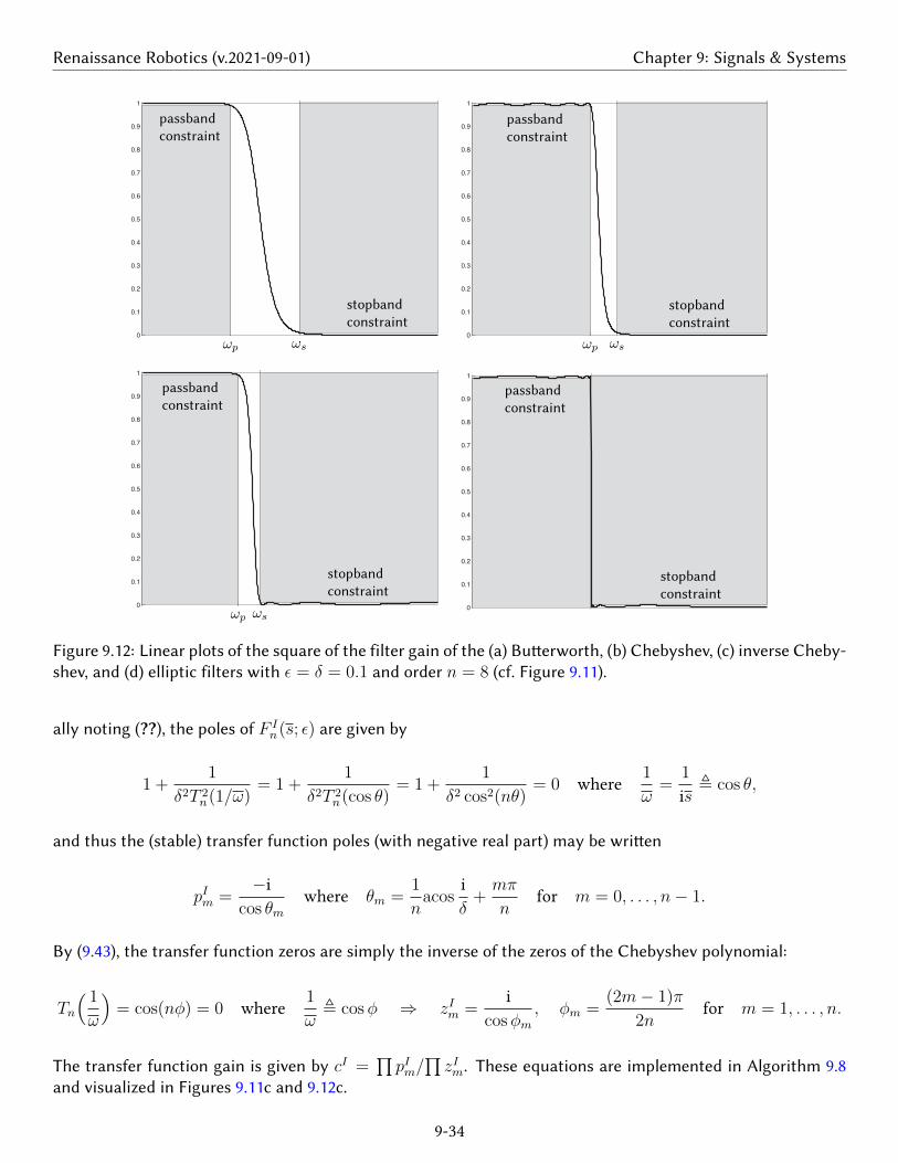
Renaissance Robotics (v.2021-09-01) Chapter 9: Signals & Systems
0
0.1
0.2
0.3
0.4
0.5
0.6
0.7
0.8
0.9
1
x
ωp ωs
passbandconstraint
stopbandconstraint
0
0.1
0.2
0.3
0.4
0.5
0.6
0.7
0.8
0.9
1
x
ωp ωs
passbandconstraint
stopbandconstraint
0
0.1
0.2
0.3
0.4
0.5
0.6
0.7
0.8
0.9
1
0
ωp ωs
passbandconstraint
stopbandconstraint
0
0.1
0.2
0.3
0.4
0.5
0.6
0.7
0.8
0.9
1
0
passbandconstraint
stopbandconstraint
Figure 9.12: Linear plots of the square of the filter gain of the (a) Buerworth, (b) Chebyshev, (c) inverse Cheby-shev, and (d) elliptic filters with ε = δ = 0.1 and order n = 8 (cf. Figure 9.11).
ally noting (??), the poles of F In(s; ε) are given by
1 +1
δ2T 2n(1/ω)
= 1 +1
δ2T 2n(cos θ)
= 1 +1
δ2 cos2(nθ)= 0 where
1
ω=
1
is, cos θ,
and thus the (stable) transfer function poles (with negative real part) may be wrien
pIm =−i
cos θmwhere θm =
1
nacos
iδ
+mπ
nfor m = 0, . . . , n− 1.
By (9.43), the transfer function zeros are simply the inverse of the zeros of the Chebyshev polynomial:
Tn
( 1
ω
)= cos(nφ) = 0 where
1
ω, cosφ ⇒ zIm =
icosφm
, φm =(2m− 1)π
2nfor m = 1, . . . , n.
The transfer function gain is given by cI =∏pIm/
∏zIm. These equations are implemented in Algorithm 9.8
and visualized in Figures 9.11c and 9.12c.
9-34
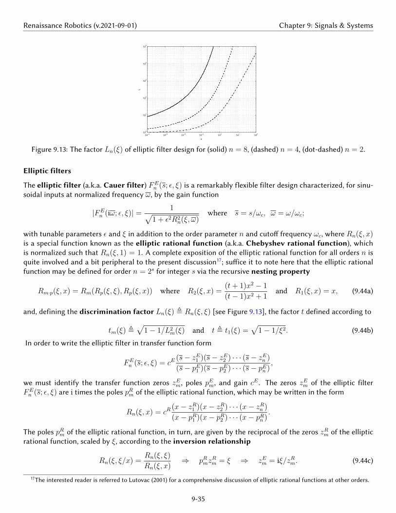
Renaissance Robotics (v.2021-09-01) Chapter 9: Signals & Systems
10−4
10−3
10−2
10−1
100
101
102
100
101
102
103
104
105
Lx
Figure 9.13: The factor Ln(ξ) of elliptic filter design for (solid) n = 8, (dashed) n = 4, (dot-dashed) n = 2.
Elliptic filters
The elliptic filter (a.k.a. Cauer filter) FEn (s; ε, ξ) is a remarkably flexible filter design characterized, for sinu-
soidal inputs at normalized frequency ω, by the gain function
|FEn (iω; ε, ξ)| = 1√
1 + ε2R2n(ξ, ω)
where s = s/ωc, ω = ω/ωc;
with tunable parameters ε and ξ in addition to the order parameter n and cuto frequency ωc, where Rn(ξ, x)is a special function known as the elliptic rational function (a.k.a. Chebyshev rational function), whichis normalized such that Rn(ξ, 1) = 1. A complete exposition of the elliptic rational function for all orders n isquite involved and a bit peripheral to the present discussion17; suice it to note here that the elliptic rationalfunction may be defined for order n = 2s for integer s via the recursive nesting property
Rm·p(ξ, x) = Rm(Rp(ξ, ξ), Rp(ξ, x)) where R2(ξ, x) =(t+ 1)x2 − 1
(t− 1)x2 + 1and R1(ξ, x) = x, (9.44a)
and, defining the discrimination factor Ln(ξ) , Rn(ξ, ξ) [see Figure 9.13], the factor t defined according to
tm(ξ) ,√
1− 1/L2m(ξ) and t , t1(ξ) =
√1− 1/ξ2. (9.44b)
In order to write the elliptic filter in transfer function form
FEn (s; ε, ξ) = cE
(s− zE1 )(s− zE2 ) · · · (s− zEn )
(s− pE1 )(s− pE2 ) · · · (s− pEn ),
we must identify the transfer function zeros zEm, poles pEm, and gain cE . The zeros zEm of the elliptic filterFEn (s; ε, ξ) are i times the poles pRm of the elliptic rational function, which may be wrien in the form
Rn(ξ, x) = cR(x− zR1 )(x− zR2 ) · · · (x− zRn )
(x− pR1 )(x− pR2 ) · · · (x− pRn ).
The poles pRm of the elliptic rational function, in turn, are given by the reciprocal of the zeros zRm of the ellipticrational function, scaled by ξ, according to the inversion relationship
Rn(ξ, ξ/x) =Rn(ξ, ξ)
Rn(ξ, x)⇒ pRmz
Rm = ξ ⇒ zEm = iξ/zRm. (9.44c)
17The interested reader is referred to Lutovac (2001) for a comprehensive discussion of elliptic rational functions at other orders.
9-35
Renaissance Robotics (v.2021-09-01) Chapter 9: Signals & Systems
For n = 2s, the zeros of Rn(ξ, x), zRm , zR,1m for m = 1, . . . , n, may be determined by initializing zR,n = 0 anditerating
[zR,2
r
m = 1/√
1 + t2r1− zR,2r+1
m
1 + zR,2r+1
m
and zR,2r
m+2s−1−r = −zR,2rm for m = 1, . . . , 2s−1−r]
for r = s−1, . . . , 0.
(9.44d)The poles pEm of the elliptic filter FE
n (s; ε, ξ) are given by pEm = (am + ibm)/cm for m = 1, . . . , n where
am = −ζn√
1− ζ2n
√1− (zRm)2
√1− (zRm)2/ξ2, bm = zRm
√1− ζ2
n(1− 1/ξ2), cm = 1− ζ2n
(1− (zRm)2
ξ2
),
(9.44e)where the ζn function may be found for n = 2s via the recursive formula
ζn(ξ, ε) = ζ2
(ξ,
√1
ζ2n/2(L2(ξ), ε)
− 1
)with ζ2(ξ, ε) =
2
(1 + t)√
1 + ε2 +√
(1− t)2 + ε2(1 + t)2. (9.44f)
The transfer function gain is given by
cE =1√
1 + ε2
∏pEm∏zEm. (9.44g)
These equations are implemented in Algorithm 9.9 and visualized in Figures 9.11d and 9.12d. Given constraintson ε and δ (see, e.g., Figures 9.11 and 9.12) and a choice for n, the necessary value for ξ may be calculated viathe discrimination factor (see Figure 9.13), using a bisection search (see Algorithm ??) to find that value of ξsuch that Ln(ξ)− 1/(εδ) = 0.
ExercisesExercise 9.1 Compute the eigenvalues and eigenvectors of the system matrixA1 in (??) (there will be three realeigenvalues and one complex conjugate pair of eigenvalues). Then, using Algorithm ??, perform a numericalsimulation of each of these modes, and explain the results. [Hint: in each of the simulations performed corre-sponding to the real modes, simply initialize the state of the system in the shape of the (real) eigenvector, thenplot how each of the states evolves in time. In the case of the pair of complex modes, initialize the state of thesystem in the shape of an appropriate linear combination of the two (complex) eigenvectors that results in a realperturbation, and again plot how each of the states evolves in time.]
Physically, the dutch roll mode of an aircraft corresponds to an oscillatory perturbation involving rst abit of roll, which creates adverse yaw towards the upward moving wing, which in turn causes a loss of lift onthe upward perturbed wing, which then causes roll in the other direction, etc.; looking aft out the top of thecockpit using a periscopic sextant (which you could do in certain vintage transport aircraft, such as the C124Old Shaky, in order to perform celestial navigation), the tail of the aircraft repeatedly draws an innity sign onthe horizon when the dutch roll mode is excited (which is, essentially, all the time); nonlinearities not discussedhere ultimately limit the magnitude of the dutch roll mode of the C124 to a nite-amplitude limit cycle. Theroll subsidence mode is an exponentially stable (and usually relatively fast) mode that quanties how muchthe aircraft continues to roll once a slight roll is initiated then the ailerons neutralized. The spiral mode isan exponentially stable (and usually relatively slow) mode coupling the yaw rate and the roll (but typically notnecessarily involving sideslip; it is often a nearly co"ordinated motion). Associate each of the simulations youperform in Exercise (9.1) to the modes characterized above, and determine the stability and damping of each.Also, there is one more (trivial) mode: physically interpret this mode as well.
9-36
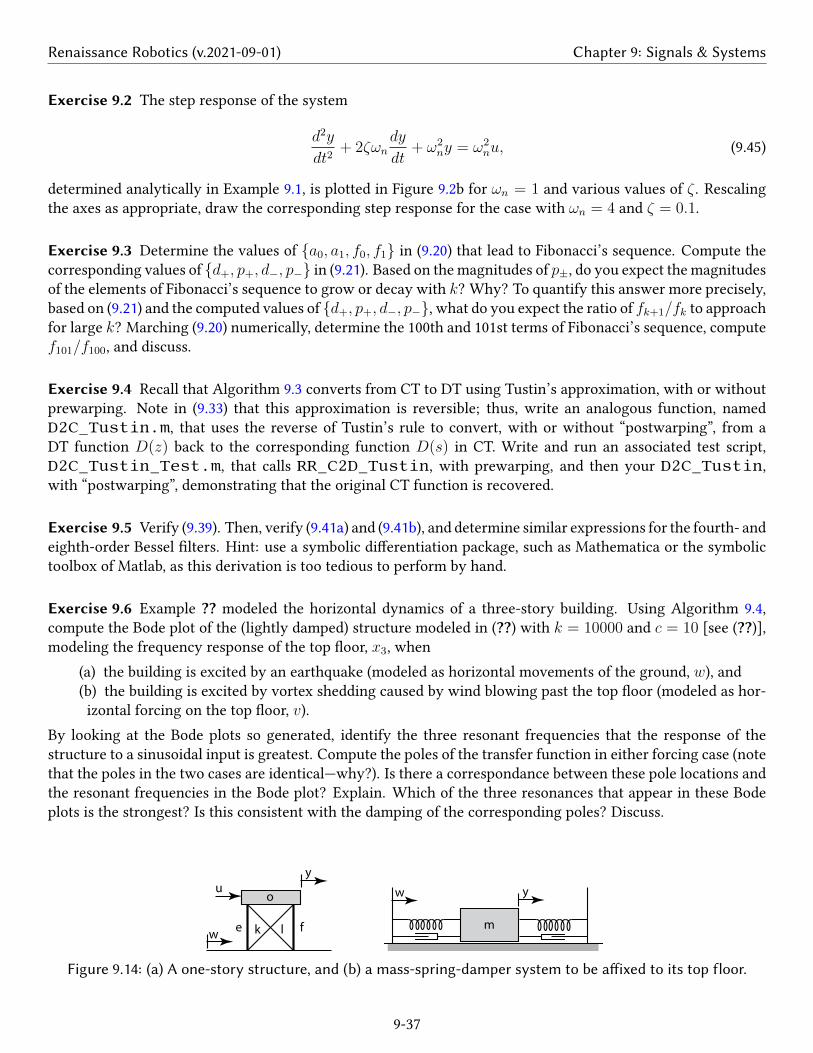
Renaissance Robotics (v.2021-09-01) Chapter 9: Signals & Systems
Exercise 9.2 The step response of the system
d2y
dt2+ 2ζωn
dy
dt+ ω2
ny = ω2nu, (9.45)
determined analytically in Example 9.1, is plotted in Figure 9.2b for ωn = 1 and various values of ζ . Rescalingthe axes as appropriate, draw the corresponding step response for the case with ωn = 4 and ζ = 0.1.
Exercise 9.3 Determine the values of a0, a1, f0, f1 in (9.20) that lead to Fibonacci’s sequence. Compute thecorresponding values of d+, p+, d−, p− in (9.21). Based on the magnitudes of p±, do you expect the magnitudesof the elements of Fibonacci’s sequence to grow or decay with k? Why? To quantify this answer more precisely,based on (9.21) and the computed values of d+, p+, d−, p−, what do you expect the ratio of fk+1/fk to approachfor large k? Marching (9.20) numerically, determine the 100th and 101st terms of Fibonacci’s sequence, computef101/f100, and discuss.
Exercise 9.4 Recall that Algorithm 9.3 converts from CT to DT using Tustin’s approximation, with or withoutprewarping. Note in (9.33) that this approximation is reversible; thus, write an analogous function, namedD2C_Tustin.m, that uses the reverse of Tustin’s rule to convert, with or without “postwarping”, from aDT function D(z) back to the corresponding function D(s) in CT. Write and run an associated test script,D2C_Tustin_Test.m, that calls RR_C2D_Tustin, with prewarping, and then your D2C_Tustin,with “postwarping”, demonstrating that the original CT function is recovered.
Exercise 9.5 Verify (9.39). Then, verify (9.41a) and (9.41b), and determine similar expressions for the fourth- andeighth-order Bessel lters. Hint: use a symbolic dierentiation package, such as Mathematica or the symbolictoolbox of Matlab, as this derivation is too tedious to perform by hand.
Exercise 9.6 Example ?? modeled the horizontal dynamics of a three-story building. Using Algorithm 9.4,compute the Bode plot of the (lightly damped) structure modeled in (??) with k = 10000 and c = 10 [see (??)],modeling the frequency response of the top oor, x3, when
(a) the building is excited by an earthquake (modeled as horizontal movements of the ground, w), and(b) the building is excited by vortex shedding caused by wind blowing past the top oor (modeled as hor-izontal forcing on the top oor, v).
By looking at the Bode plots so generated, identify the three resonant frequencies that the response of thestructure to a sinusoidal input is greatest. Compute the poles of the transfer function in either forcing case (notethat the poles in the two cases are identical—why?). Is there a correspondance between these pole locations andthe resonant frequencies in the Bode plot? Explain. Which of the three resonances that appear in these Bodeplots is the strongest? Is this consistent with the damping of the corresponding poles? Discuss.
o
y
u
we fk l
w
m
y
Figure 9.14: (a) A one-story structure, and (b) a mass-spring-damper system to be aixed to its top floor.
9-37
Renaissance Robotics (v.2021-09-01) Chapter 9: Signals & Systems
Exercise 9.7 Simplifying the linearized model considered in Example ??, a one-story building (Figure 9.14a) inwhich the top oor has horizontal position y, applied force v, and mass M is governed by
Md2y
dt2= v −K(y − w)− C
(dydt− dw
dt
), (9.46a)
where K and C denote the eective spring and damping coecients of the linearized structure, and w denotesthe horizontal position of the ground. Extending the mass-spring-damper model considered in Example ?? toaccount for a moving wall, a single mass-spring-damper system (Figure 9.14b) in which the mass has horizontalposition x and the wall has horizontal position y is governed by
md2x
dt2= −k(x− y)− c
(dxdt− dy
dt
), (9.46b)
where k/2 and c/2 are the coecients of the spring and damper mounted on each side of the mass.We consider now the problem of mounting the mass-spring-damper system to the top of the one-story
structure, so the y in (9.46a) corresponds precisely to the y in (9.46b), and the reaction force v on the top of thebuilding from the mass-spring-damper system is precisely the negative of the RHS of (9.46b); that is,
v = k(x− y) + c(dxdt− dy
dt
). (9.46c)
(a) Taking the Laplace transform of (9.46a)-(9.46c), assuming the system starts at rest, compute L1, L2, L3, andL4 as a function of M , K , C , m, k, c, and s in the following (transformed) representation of these equations:
L1Y (s) = V (s) + L2W (s), (9.47a)
L3X(s) = L4Y (s), (9.47b)
V (s) = L4X(s)− L4Y (s). (9.47c)
Now, premultiply (9.47b) by L4 and (9.47c) by L3 and, noting that L3L4 = L4L3, substitute the former into thelatter to eliminate X(s). Then substitute the resulting equation into L3 times (9.47a) to eliminate V (s). Theresult may be written in transfer-function form as
L5Y (s) = L6W (s) ⇒ Y (s)
W (s)=L6
L5
(9.48)
(b) Compute L5 and L6 in terms ofM ,K , C ,m, k, c, and the Laplace transform variable s. Is this system strictlyproper, semiproper, or improper? How many poles and (nite) zeros are there in this system?(c) Taking m = 0, simplify (9.48); is the result what you expect? Explain.(d) In addition to taking m = 0, assume further that M = K = 10 and C = 0. Where are the poles and zeros ofG(s) in this case? Plot the Bode plot of this system.(e) Taking w(t) = δλ,m(t) for λ → ∞, and thus W (s) = 1, calculate the impulse response of the systemconsidered in part (d) exactly, by hand, using partial fraction expansion and inverse Laplace transform, notingthe Laplace transforms listed in Table 9.1. Accurately plot this impulse response. Then, taking w(t) as a unitstep, and thus W (s) = 1/s, calculate and plot the step response of this system in the same manner.(f) Taking C = 10
√2 = 14.14, repeat parts (d) and (e) in their entirety.
(g) Now taking M = K = 10, C = 0, and m = 1, k = 9, c = 0 in (9.48), compute the poles of G(s) by hand(hint: the denominator is now quadratic in s2). Have the slowest poles, corresponding to the pole locationsidentied in part (d), without the spring/mass/damper system mounted atop the structure, moved? Discuss.
9-38
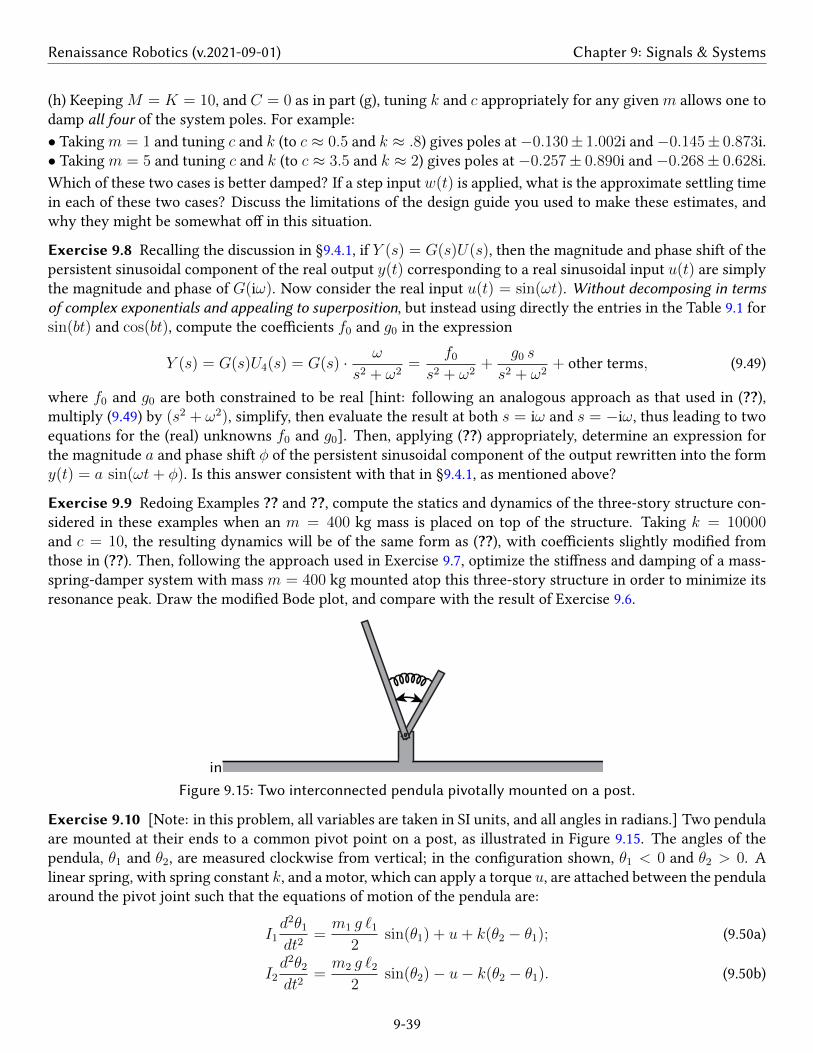
Renaissance Robotics (v.2021-09-01) Chapter 9: Signals & Systems
(h) Keeping M = K = 10, and C = 0 as in part (g), tuning k and c appropriately for any given m allows one todamp all four of the system poles. For example:• Taking m = 1 and tuning c and k (to c ≈ 0.5 and k ≈ .8) gives poles at−0.130± 1.002i and−0.145± 0.873i.• Taking m = 5 and tuning c and k (to c ≈ 3.5 and k ≈ 2) gives poles at −0.257± 0.890i and −0.268± 0.628i.Which of these two cases is better damped? If a step input w(t) is applied, what is the approximate settling timein each of these two cases? Discuss the limitations of the design guide you used to make these estimates, andwhy they might be somewhat o in this situation.
Exercise 9.8 Recalling the discussion in §9.4.1, if Y (s) = G(s)U(s), then the magnitude and phase shift of thepersistent sinusoidal component of the real output y(t) corresponding to a real sinusoidal input u(t) are simplythe magnitude and phase of G(iω). Now consider the real input u(t) = sin(ωt). Without decomposing in termsof complex exponentials and appealing to superposition, but instead using directly the entries in the Table 9.1 forsin(bt) and cos(bt), compute the coecients f0 and g0 in the expression
Y (s) = G(s)U4(s) = G(s) · ω
s2 + ω2=
f0
s2 + ω2+
g0 s
s2 + ω2+ other terms, (9.49)
where f0 and g0 are both constrained to be real [hint: following an analogous approach as that used in (??),multiply (9.49) by (s2 + ω2), simplify, then evaluate the result at both s = iω and s = −iω, thus leading to twoequations for the (real) unknowns f0 and g0]. Then, applying (??) appropriately, determine an expression forthe magnitude a and phase shift φ of the persistent sinusoidal component of the output rewritten into the formy(t) = a sin(ωt+ φ). Is this answer consistent with that in §9.4.1, as mentioned above?
Exercise 9.9 Redoing Examples ?? and ??, compute the statics and dynamics of the three-story structure con-sidered in these examples when an m = 400 kg mass is placed on top of the structure. Taking k = 10000and c = 10, the resulting dynamics will be of the same form as (??), with coecients slightly modied fromthose in (??). Then, following the approach used in Exercise 9.7, optimize the stiness and damping of a mass-spring-damper system with mass m = 400 kg mounted atop this three-story structure in order to minimize itsresonance peak. Draw the modied Bode plot, and compare with the result of Exercise 9.6.
inFigure 9.15: Two interconnected pendula pivotally mounted on a post.
Exercise 9.10 [Note: in this problem, all variables are taken in SI units, and all angles in radians.] Two pendulaare mounted at their ends to a common pivot point on a post, as illustrated in Figure 9.15. The angles of thependula, θ1 and θ2, are measured clockwise from vertical; in the conguration shown, θ1 < 0 and θ2 > 0. Alinear spring, with spring constant k, and a motor, which can apply a torque u, are attached between the pendulaaround the pivot joint such that the equations of motion of the pendula are:
I1d2θ1
dt2=m1 g `1
2sin(θ1) + u+ k(θ2 − θ1); (9.50a)
I2d2θ2
dt2=m2 g `2
2sin(θ2)− u− k(θ2 − θ1). (9.50b)
9-39

Renaissance Robotics (v.2021-09-01) Chapter 9: Signals & Systems
The pendula may be idealized as simple rods with masses m1 = 1 and m2 = 3 and lengths `1 = 2 and `2 = 1and inertias I1 = m1`
21/3 and I2 = m2`
22/3, and we take g ≈ 10 and k = 6.
(a) Linearize (9.50) about a possibly time-varying nominal state θ1(t), θ2(t), u(t), which itself solves (9.50),by taking θ1 = θ1 + θ′1, θ2 = θ2 + θ′2, and u = u + u′ in (9.50), noting (??), (??), and (??), and, assuming theperturbation θ′1, θ′2, u′ is small, identifying a linear equation governing θ′1, θ′2, u′.
(b) Taking θ1 = θ1, θ2 = θ2, and u = u in (9.50) and assuming additionally that this nominal state is anequilibrium state (that is, dθ1/dt = dθ2/dt = 0), derive an equation that relates θ1 and θ2 (do not yet assume that|θ1| or |θ2| is small). Also, determine an expression for the corresponding u required to hold this equilibriumstate as a function of θ1 only. What is the largest value of |θ2| that can be held in equilibrium? If |θ1| and |θ2|are both small, what is the relationship between them in equilibrium?
(c) Linearizing (9.50a)-(9.50b) about the zero state θ1 = θ2 = u = 0, compute the transfer function G(s) =Θ′2(s)/U ′(s). Where are the poles and zeros of this transfer function? (Note: we will consider the stabilization ofthis pathological unstable system in §??.) Using the Table 9.1a, compute the response of this linearized system,θ′2(t), to a unit impulse u′(t) = δ(t) [and, thus, U ′(s) = 1].
(d) Identify appropriate values of the physical parameters m1, m2, `1, and `2 such that the transfer functionof this system has zeros at s = ±2 and poles at s = ±1 and ±3.
Exercise 9.11 Sketch (using the rules of §9.4.1.1) and plot (using Matlab) the Bode plots of the following transferfunctions, and identify whether each is strictly proper, semi proper, or improper:
(a) the (rst-order) low-pass filter G1(s) =1
s+ 1;
(b) the PD filter G2(s) =s− 1
1;
(c) the all-pass filter G3(s) =s− 1
s+ 1= G1(s)G2(s) [appeal to Fact 9.15 together with (a) and (b) above];
(d) the PID filter G4(s) =s2 + 101s+ 100
s;
(e) the bandpass filter G5(s) =s
s2 + 101s+ 100;
(f) the (second-order) low-pass filter G6(s) =1
s2 + s+ 1.
Exercise 9.12 Consider a DT system with transfer function
Y (z)
U(z)= G(z) =
1
z2 − 0.1z(9.51)
(a) Compute the poles z1 and z2 of (9.51). Is this system stable, neutrally stable, or unstable? Explain.(b) Compute the dierence equation corresponding to (9.51). Assuming the system starts out at rest (that is,
yk = 0 for k < 0) and that uk = δ0k, evaluate directly the response of this system for k = 0, 1, 2, 3, 4. Repeat foruk = h0k [see (??)].
(c) Taking an impulse input uk = δ0k [that is, taking U(z) = 1 in (9.51)], compute c1, c2 in the partialfraction expansion
Y (z) = G(z)U(z) =c1
z − z1
+c2
z − z2
. (9.52)
Applying Table 9.1b to this result, compute the impulse response of (9.51) for all k. Evaluate the resulting ex-pression for k = 0, 1, 2, 3, 4; does the result match the corresponding calculation in (b)? What does yk approachas k →∞? Is this consistent with Fact 9.11 applied to Y (z) in (9.51) when U(z) = 1?
9-40
Renaissance Robotics (v.2021-09-01) Chapter 9: Signals & Systems
(d) Taking a step input uk = h0k [that is, taking, U(z) = z/(z − 1) in (9.51)], compute d1, d2, d3 in thepartial fraction expansion
Y (z) = G(z)U(z) =d1
z − z1
+d2
z − z2
+d3
z − 1. (9.53)
Applying Table 9.1b to this result, compute the step response of (9.51) for all k. Evaluate the resulting expressionfor k = 0, 1, 2, 3, 4; does the result match the corresponding calculation in (b)? What does yk approach ask →∞? Is this consistent with Fact 9.11 applied to Y (z) in (9.51) when U(z) = z/(z − 1)?
ReferencesFranklin, G, Powell, JD, & Emami-Naeini, A (2006) Feedback Control of Dynamic Systems, Prentice Hall.
Gillespie, TD (1992) Fundamentals of Vehicle Dynamics, SAE.
LePage, WR (1961) Complex Variables and the Laplace Transform for Engineers, Dover.
Minto, KD, Chow, JH, Beseler, J (1989) Lateral Axis Autopilot Design For Large Transport Aircra: An ExplicitModel-Matching Approach American Control Conference, 585-591.
Stevens, BL, & Lewis, FL (2003) Aircra Control and Simulation. Wiley.
9-41

Renaissance Robotics (v.2021-09-01) Chapter 9: Signals & Systems
9-42