Water Pumps

The Islamic University of GazaFaculty of Engineering

Civil Engineering Department

Hydraulics - ECIV 3322

Chapter 5Chapter 5

Definition

• Water pumps are devices designed to convert mechanical energy to hydraulic energy.

• They are used to move water from lower points to higher points with a required discharge and pressure head.

• This chapter will deal with the basic hydraulic concepts of water pumps

Pump Classification

• Turbo-hydraulic (kinetic) pumpsCentrifugal pumps (radial-flow pumps)Propeller pumps (axial-flow pumps)Jet pumps (mixed-flow pumps)• Positive-displacement pumps Screw pumpsReciprocating pumps

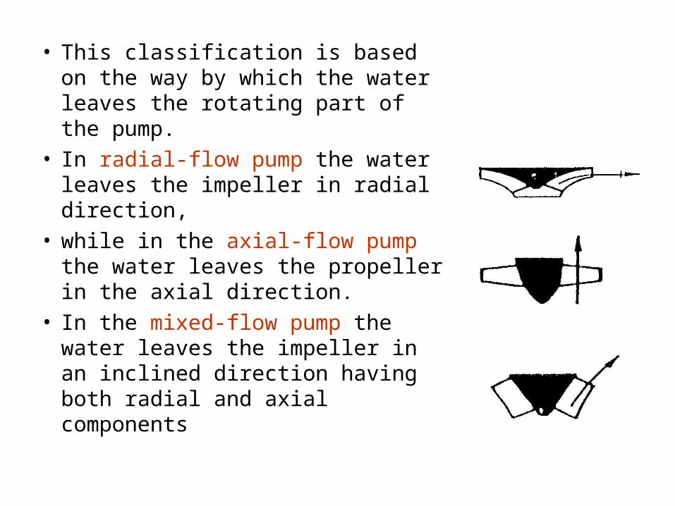
• This classification is based on the way by which the water leaves the rotating part of the pump.

• In radial-flow pump the water leaves the impeller in radial direction,

• while in the axial-flow pump the water leaves the propeller in the axial direction.

• In the mixed-flow pump the water leaves the impeller in an inclined direction having both radial and axial components

Schematic diagram of basic elements of centrifugal

pump

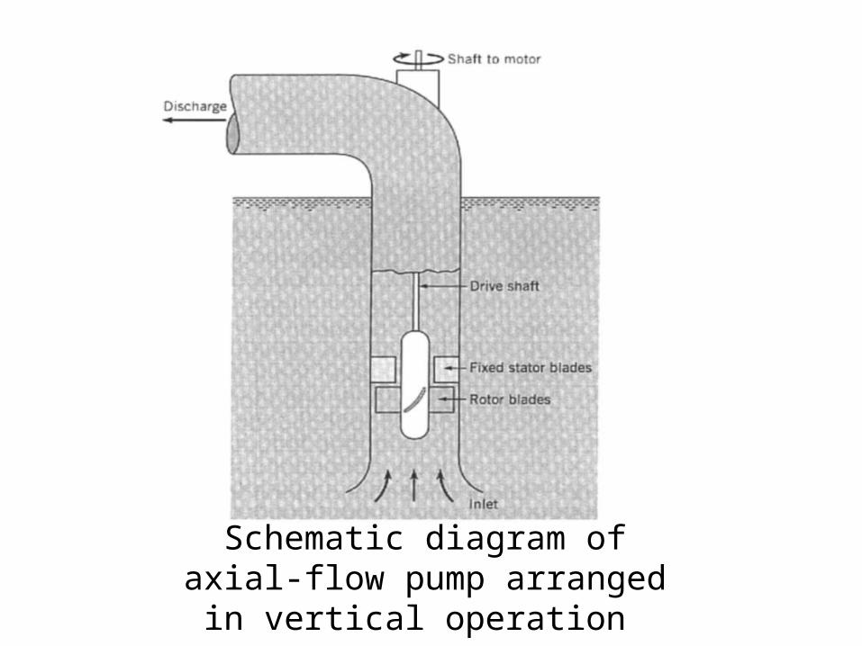
Schematic diagram of axial-flow pump arranged in vertical operation

Screw pumps.

• In the screw pump a revolving shaft fitted with blades rotates in an inclined trough and pushes the water up the trough.

Reciprocating pumps.• In the reciprocating pump a piston sucks the

fluid into a cylinder then pushes it up causing the water to rise.

تبارك الله أحسن الخالقين

Centrifugal Pumps

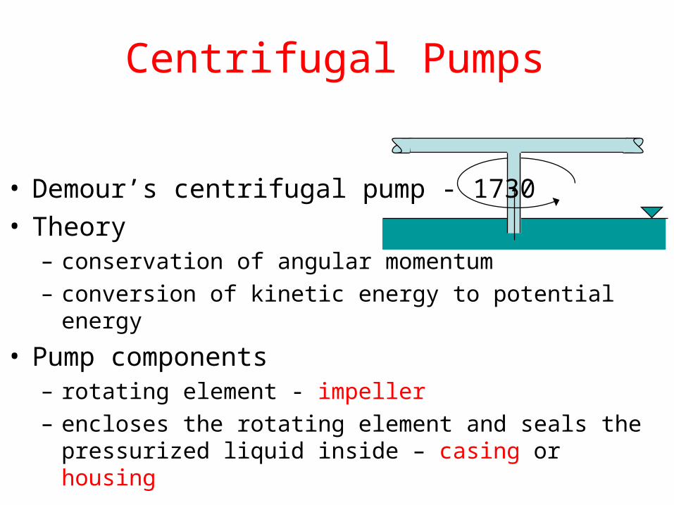
• Demour’s centrifugal pump - 1730• Theory

– conservation of angular momentum– conversion of kinetic energy to potential energy

• Pump components– rotating element - impeller– encloses the rotating element and seals the pressurized

liquid inside – casing or housing

Centrifugal Pumps

ImpellerVanes

CasingSuction Eye Impeller

DischargeFlow Expansion

• Broad range of applicable flows and heads• Higher heads can be achieved by increasing the

diameter or the rotational speed of the impeller

Centrifugal Pump:

• Centrifugal pumps (radial-flow pumps) are the most used pumps for hydraulic purposes. For this reason, their hydraulics will be studied in the following sections.

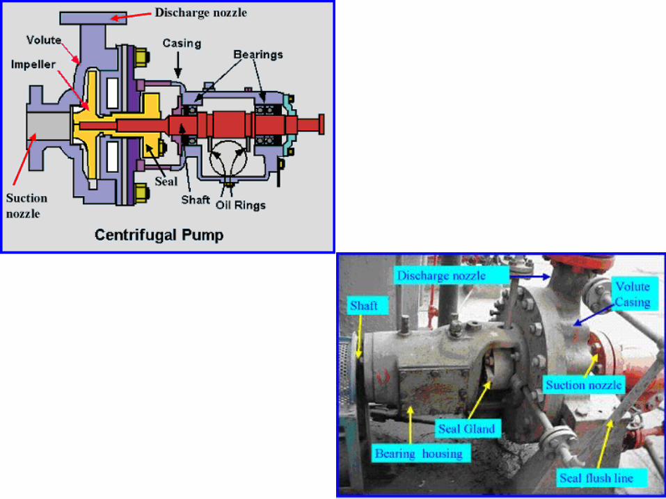
Main Parts of Centrifugal Pumps

• which is the rotating part of the centrifugal pump.

• It consists of a series of backwards curved vanes (blades).

• The impeller is driven by a shaft which is connected to the shaft of an electric motor.

1. Impeller:

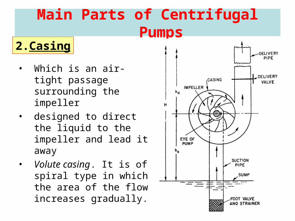
Main Parts of Centrifugal Pumps

• Which is an air-tight passage surrounding the impeller

• designed to direct the liquid to the impeller and lead it away

• Volute casing. It is of spiral type in which the area of the flow increases gradually.

2. Casing

3. Suction Pipe. 4. Delivery Pipe. 5. The Shaft: which is the bar by which the

power is transmitted from the motor drive to the impeller.

6. The driving motor: which is responsible for rotating the shaft. It can be mounted directly on the pump, above it, or adjacent to it.

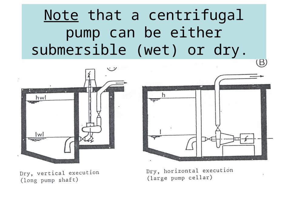
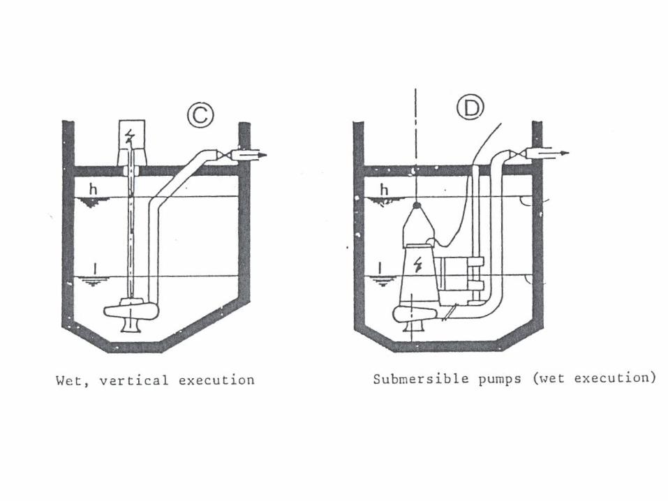
Note that a centrifugal pump can be either submersible (wet) or dry.

Hydraulic Analysis of Pumps and Piping Systems

• Pump can be placed in two possible position in reference to the water levels in the reservoirs.

• We begin our study by defining all the different terms used to describe the pump performance in the piping system.

Hydraulic Analysis of Pumps and Piping Systems

H t

hd

H st

at

h s

H m

s

H m

d

Datum pump center line

h fs

h f

d

Case 1

H st

at

H m

dH

ms

hd

H t

h s

Datum pump center line

h f

d

h f

s

Case 2

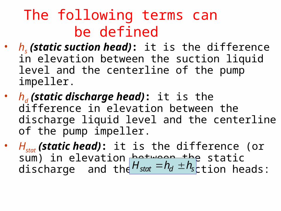
The following terms can be defined

• hs (static suction head): it is the difference in elevation between the suction liquid level and the centerline of the pump impeller.

• hd (static discharge head): it is the difference in elevation between the discharge liquid level and the centerline of the pump impeller.

• Hstat (static head): it is the difference (or sum) in elevation between the static discharge and the static suction heads: H h hstat d s

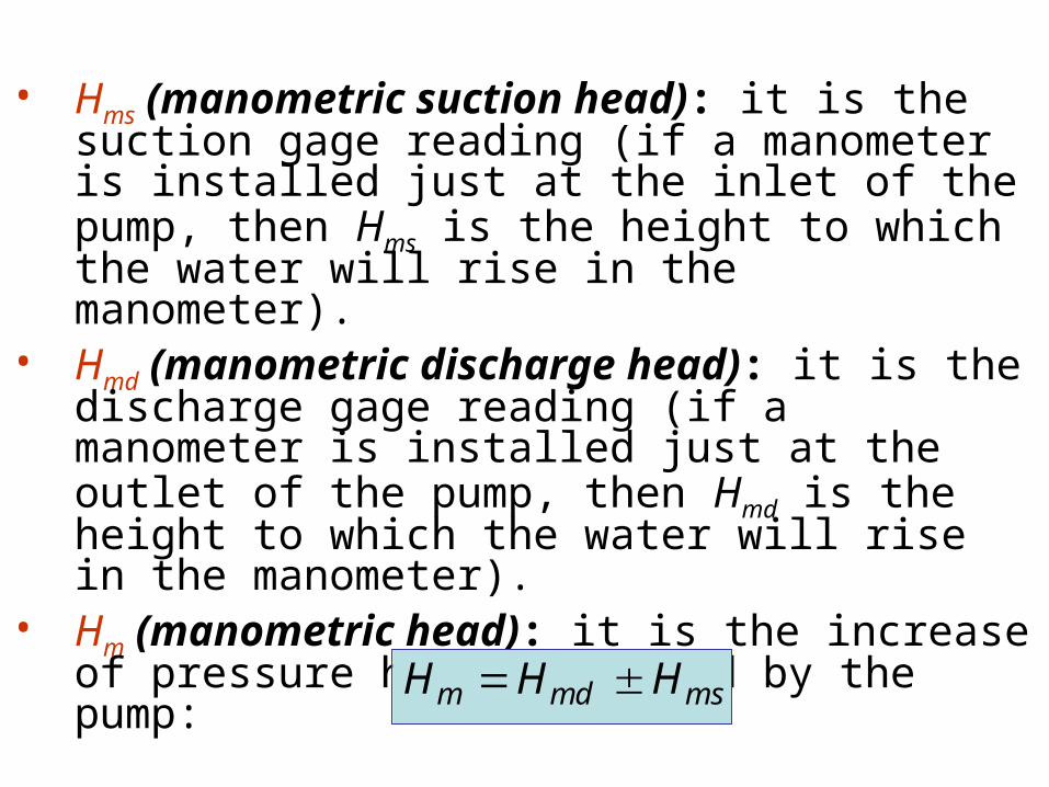
• Hms (manometric suction head): it is the suction gage reading (if a manometer is installed just at the inlet of the pump, then Hms is the height to which the water will rise in the manometer).

• Hmd (manometric discharge head): it is the discharge gage reading (if a manometer is installed just at the outlet of the pump, then Hmd is the height to which the water will rise in the manometer).

• Hm (manometric head): it is the increase of pressure head generated by the pump:

H H Hm md ms

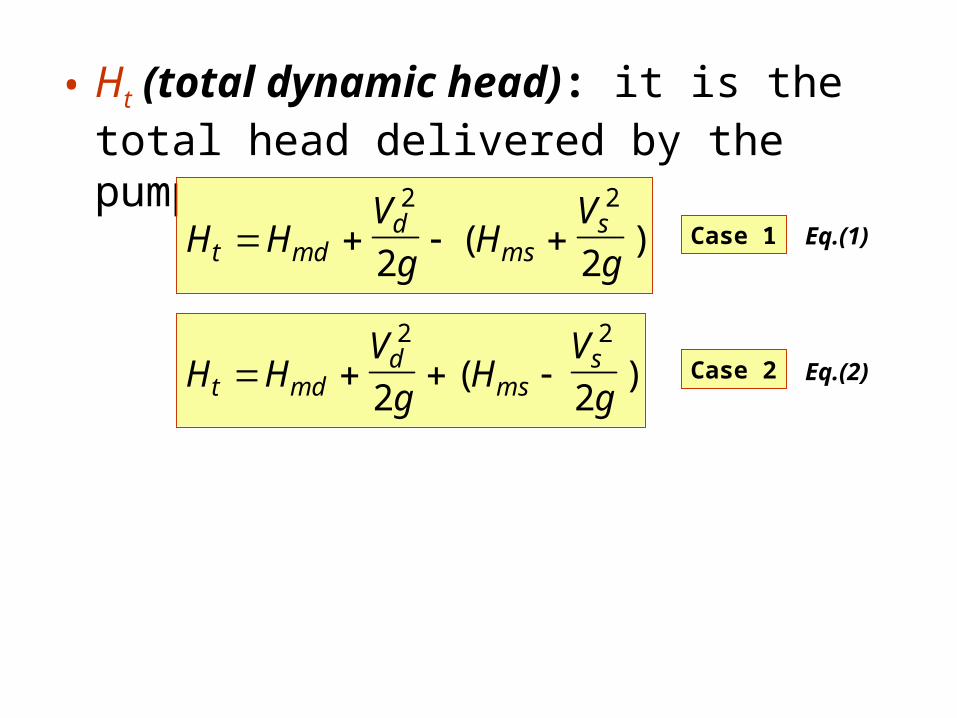
• Ht (total dynamic head): it is the total head delivered by the pump:

H HV

gH

Vgt md

dm s

s 2 2

2 2( )

H HV

gH

Vgt m d

dm s

s 2 2

2 2( )

Case 1

Case 2

Eq.(1)

Eq.(2)

• Ht can be written in another form as follows:

H h h hmd d f d md

H h h hV

gms s f s mss 2

2

H h h hV

gms s f s mss 2

2

Case 1

Case 2

H h h hV

gh h h

Vg

Vgt d f d md

ds f s ms

s s

2 2 2

2 2 2

H h hstat d s but

H H h h h hV

gt stat f d md f s msd 2

2

Substitute ino eq. (1)

Eq.(3)Case 1

• Equation (3) can be applied to Case 2 with the exception that : H h hstat d s

In the above equations; we define:hfs : is the friction losses in the suction pipe. hfd : is the friction losses in the discharge (delivery) pipe.hms : is the minor losses in the suction pipe.hmd: is the minor losses in the discharge (delivery) pipe.

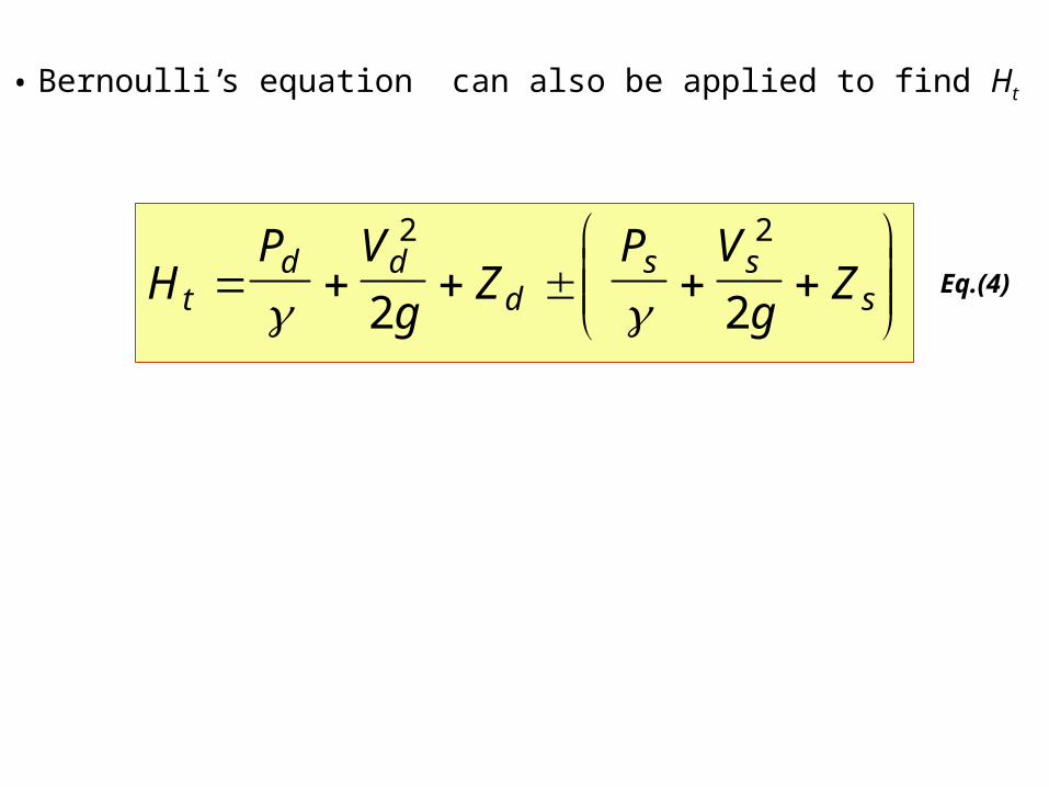
• Bernoulli’s equation can also be applied to find Ht

HP V

gZ

P Vg

Ztd d

ds s

s

2 2

2 2Eq.(4)

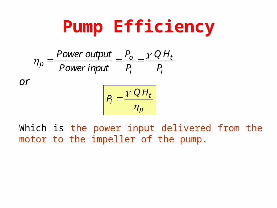
Pump Efficiency

p

o

i

t

i

Power outputPower input

PP

Q HP

PQ H

it

p

or

Which is the power input delivered from the motor to the impeller of the pump.

Motor efficiency : m

mi

m

PP

PP

mi

m

which is the power input delivered to the motor.

o

o p m

oo

m

PP

Overall efficiency of the motor-pump system:

Cavitation of Pumps and NPSH

• In general, cavitation occurs when the liquid pressure at a given location is reduced to the vapor pressure of the liquid.

• For a piping system that includes a pump, cavitation occurs when the absolute pressure at the inlet falls below the vapor pressure of the water.

• This phenomenon may occur at the inlet to a pump and on the impeller blades, particularly if the pump is mounted above the level in the suction reservoir.

• Under this condition, vapor bubbles form (water starts to boil) at the impeller inlet and when these bubbles are carried into a zone of higher pressure, they collapse abruptly and hit the vanes of the impeller (near the tips of the impeller vanes). causing:

• Damage to the pump (pump impeller)• Violet vibrations (and noise).• Reduce pump capacity.• Reduce pump efficiency

• To avoid cavitation, the pressure head at the inlet should not fall below a certain minimum which is influenced by the further reduction in pressure within the pump impeller.

• To accomplish this, we use the difference between the total head at the inlet , and the water vapor pressure head

gVP ss

2

2

vaporP

How we avoid Cavitation ??

Where we take the datum through the centerline of the pump impeller inlet (eye). This difference is called the Net Positive Suction Head (NPSH), so that

NPSHP V

g

Ps s vapor

2

2There are two values of NPSH of interest. The first is the required NPSH, denoted (NPSH)R , that must be maintained or exceeded so that cavitation will not occur and usually determined experimentally and provided by the manufacturer. The second value for NPSH of concern is the available NPSH, denoted (NPSH)A , which represents the head that actually occurs for the particular piping system. This value can be determined experimentally, or calculated if the system parameters are known.

How we avoid Cavitation ??

• For proper pump operation (no cavitation) :

(NPSH)A > (NPSH)R

Determination of (NPSH)A

datum

hs

applying the energy equation between point (1) and (2), datum at pump center line

VaporLS

atmA

VaporLS

atmVaporSS

LSatmSS

LSS

Satm

PhhPNPSH

PhhPP

gVP

hhPg

VP

hg

VPhP

)(

2

2

2

2

2

2

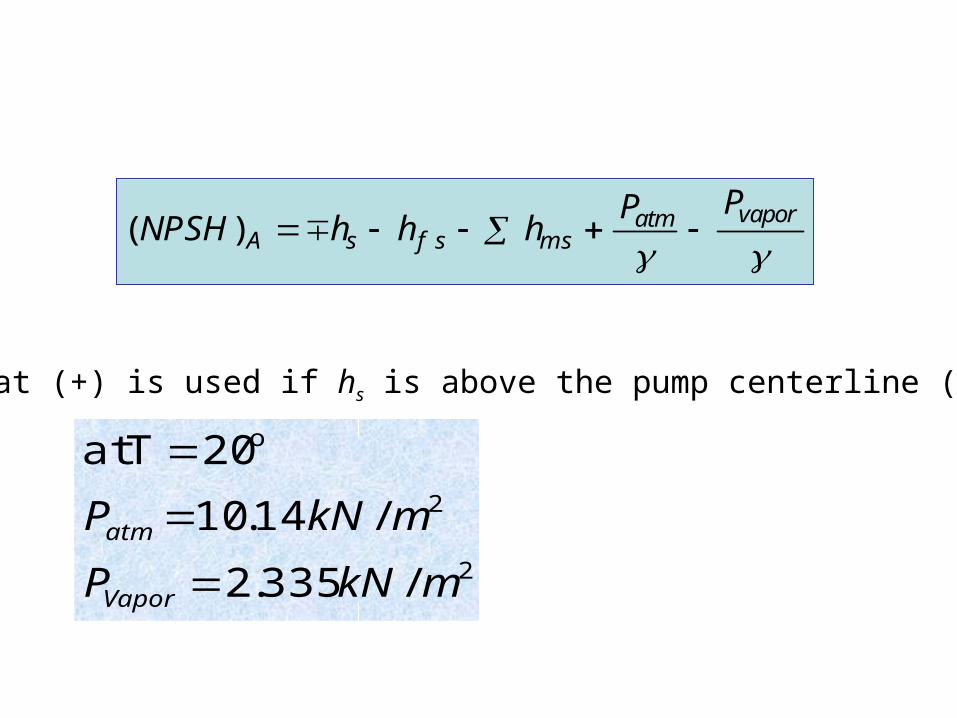
( )NPSH h h hP P

A s f s m satm vapor

Note that (+) is used if hs is above the pump centerline (datum).

2

2

o

/ 335.2

/ 14.10

20Tat

mkNP

mkNP

Vapor

atm

Thoma’s cavitation constant

The cavitation constant: is the ratio of (NPSH)R to the total dynamic head (Ht) is known as the Thoma’s cavitation constant ( )

( )NPSH

HR

t

Note: If the cavitation constant is given, we can find the maximum allowable elevation of the pump inlet (eye) above the surface of the supply (suction) reservoir.

Selection of A Pump It has been seen that the efficiency of a pump depends on the discharge, head, and power requirement of the pump. The approximate ranges of application of each type of pump are indicated in the following Figure.

Selection of A Pump

• In selecting a particular pump for a given system: • The design conditions are specified and a pump is selected

for the range of applications. • A system characteristic curve (H-Q) is then prepared. • The H-Q curve is then matched to the pump characteristics

chart which is provided by the manufacturer. • The matching point (operating point) indicates the actual

working conditions.

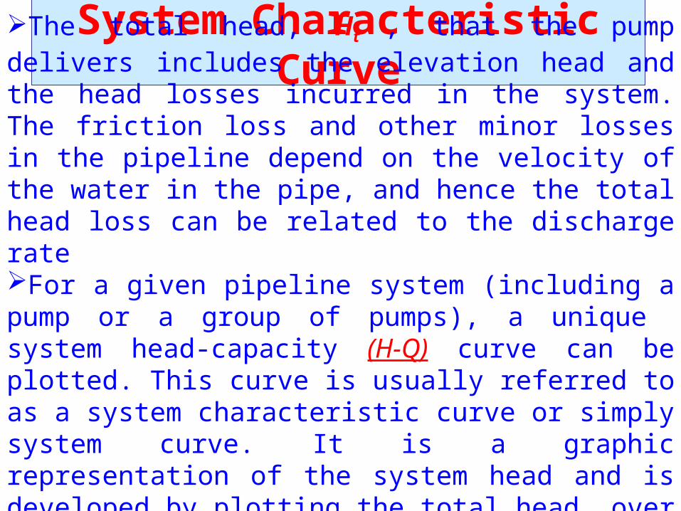
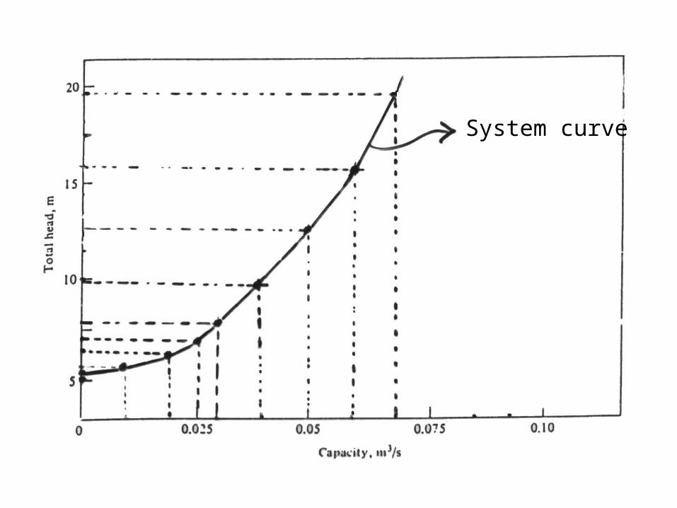
System Characteristic CurveThe total head, Ht , that the pump delivers

includes the elevation head and the head losses incurred in the system. The friction loss and other minor losses in the pipeline depend on the velocity of the water in the pipe, and hence the total head loss can be related to the discharge rateFor a given pipeline system (including a pump or a group of pumps), a unique system head-capacity (H-Q) curve can be plotted. This curve is usually referred to as a system characteristic curve or simply system curve. It is a graphic representation of the system head and is developed by plotting the total head, over a range of flow rates starting from zero to the maximum expected value of Q.

Lstatt hHH

)()( 12 QfnzzH p

systemsystem curve

0

20

40

60

80

100

120

0 0.2

0.4

0.6

0.8Discharge (m3/s)

Head

(m)

Static head (z2-z1)

System with valve partially closed

System Characteristic Curve

H H ht stat L

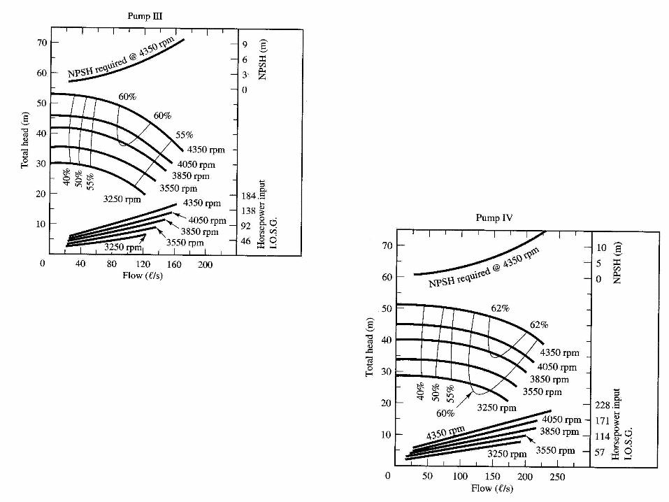
Pump Characteristic Curves

• Pump manufacturers provide information on the performance of their pumps in the form of curves, commonly called pump characteristic curves (or simply pump curves).

• In pump curves the following information may be given:• the discharge on the x-axis,• the head on the left y-axis,• the pump power input on the right y-axis,• the pump efficiency as a percentage,• the speed of the pump (rpm = revolutions/min).• the NPSH of the pump.

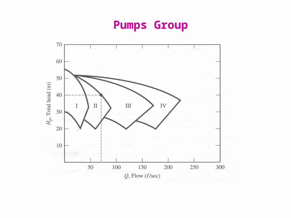
Pumps Group

• The pump characteristic curves are very important to help select the required pump for the specified conditions.

• If the system curve is plotted on the pump curves in we may produce the following Figure:

• The point of intersection is called the operating point. • This matching point indicates the actual working conditions,

and therefore the proper pump that satisfy all required performance characteristic is selected.

Matching the system and pump curves.

System Characteristic Curve

H H ht stat L

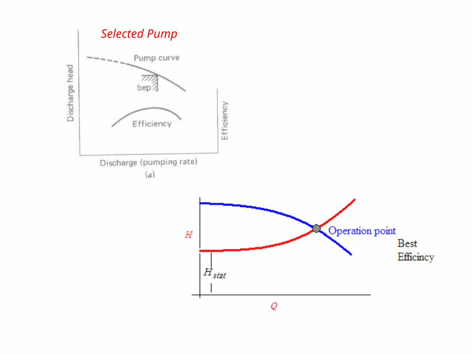
Selected Pump

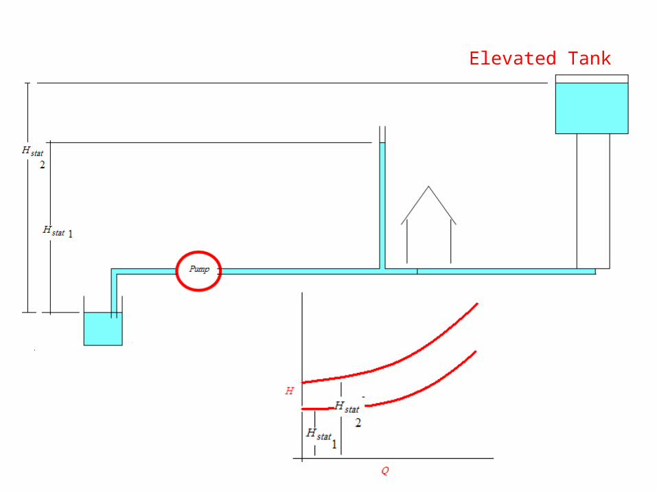
Elevated Tank

Selected Pump

System Curve & Pump Curve cases

Pump Curve

Pump Curve

Pump Curve

System Curve

System Curve

System Curve

Example 1A Pump has a cavitation constant = 0.12, this pump was instructed on well using UPVC pipe of 10m length and 200mm diameter, there are elbow (ke=1) and valve (ke=4.5) in the system. the flow is 35m3

and The total Dynamic Head Ht = 25m (from pump curve) f=0.0167Calculate the maximum suction head

mm2.0head pressureVapour

69.9head pressure atm.

325120120

.HσNPSH.σ

tR

m.g

..g

V.h SV 2830

211154

254

22

06302111

2

22

.g

.g

Vh Se

m.g

..

.g

VDLfh fS 0530

2111

201001670

2

22

m.h

....hγ

Pγ

Phhh(NPSH)

S

S

VaporatmmSf SSA

08862069.90630283005303

γP

γPhhh(NPSH) Vaporatm

mSf SSA

m/s .

.π.

AQVS 111

204

03502

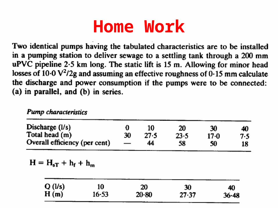
Example 2For the following pump, determine the required pipes diameter to pump 60 L/s and also calculate the needed power.Minor losses 10 v2/2gPipe length 10 kmroughness = 0.15 mmHs = 20 m

Q L/s

70 60 50 40 30 20 10 0

Ht 31 35 38 40.6 42.5 43.7 44.7 45

40 53 60 60 57 50 35 -P

To get 60 L/s from the pump Hs + hL must be < 35 m

Assume the diameter = 300mmThen:

mh

fDKR

smVmA

f

Se

32.2362.193.0

85.010000019.0

019.0,0005.0/,1025.2

/85.0,070.0

2

5

2

mgg

Vhm 37.02

85.0102

10 22

mmhhh mfs 3569.43

Assume the diameter = 350mmThen:

smVmA /624.0,0962.0 2

,48.100185.0,00043.0/,1093.1 5

mhfDKR

f

Se

mgg

Vhm 2.02

624.0102

10 22

mmhhh mfs 3568.30

kWWHQPp

ti 87.388.38869

53.03581.91000 1000

60

Example 3A pump was designed to satisfy the following system Q (m3/hr) 3 6 9

hf (m) 12 20 38

mm25.0head pressureVapour

3.10head pressure atm.

mhd 13

Pipe diameter is 50mm

gVhL 2

24Partsuction 2

Check whether the pump is suitable or not

1- Draw the system curve and check the operation point

20m713hhH SdSTAT

There are an operation point at:

Q = 9 m3/hr H =58m

NPSHR =4.1Then Check NPSHA

m.g.h

m/s..π

/AQV

L 022

27124

271050

4

36009

2

2

4.11.05(NPSH)0.2510.327(NPSH)

γP

γPhhh(NPSH)

A

A

VaporatmmSS SA

f

pump is not suitable, the cavitation will occur

Multiple-Pump Operation

• To install a pumping station that can be effectively operated over a large range of fluctuations in both discharge and pressure head, it may be advantageous to install several identical pumps at the station.

Pumps in Parallel Pumps in Series

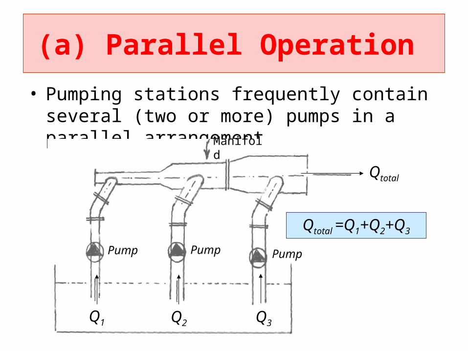
(a) Parallel Operation • Pumping stations frequently contain several (two or

more) pumps in a parallel arrangement.

Q1 Q2 Q3

Pump PumpPump

Manifold

Qtotal

Qtotal =Q1+Q2+Q3

• In this configuration any number of the pumps can be operated simultaneously.

• The objective being to deliver a range of discharges, i.e.; the discharge is increased but the pressure head remains the same as with a single pump.

• This is a common feature of sewage pumping stations where the inflow rate varies during the day.

• By automatic switching according to the level in the suction reservoir any number of the pumps can be brought into operation.

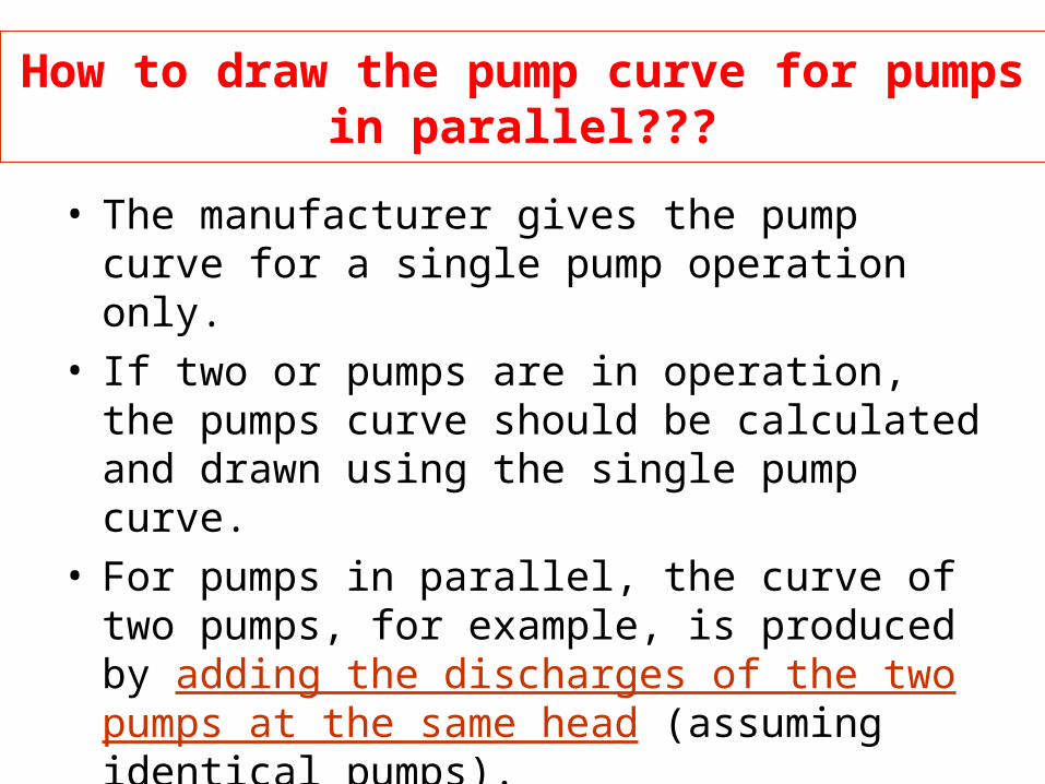
How to draw the pump curve for pumps in parallel???

• The manufacturer gives the pump curve for a single pump operation only.

• If two or pumps are in operation, the pumps curve should be calculated and drawn using the single pump curve.

• For pumps in parallel, the curve of two pumps, for example, is produced by adding the discharges of the two pumps at the same head (assuming identical pumps).

Pumps in series & Parallel

Pumps in Parallel:

mnm3m2m1m

nj

1jn321

HHHHH

QQQQQQ

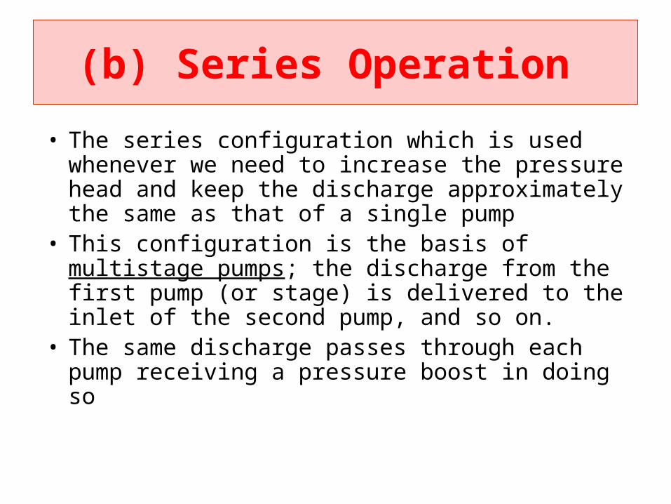
(b) Series Operation

• The series configuration which is used whenever we need to increase the pressure head and keep the discharge approximately the same as that of a single pump

• This configuration is the basis of multistage pumps; the discharge from the first pump (or stage) is delivered to the inlet of the second pump, and so on.

• The same discharge passes through each pump receiving a pressure boost in doing so

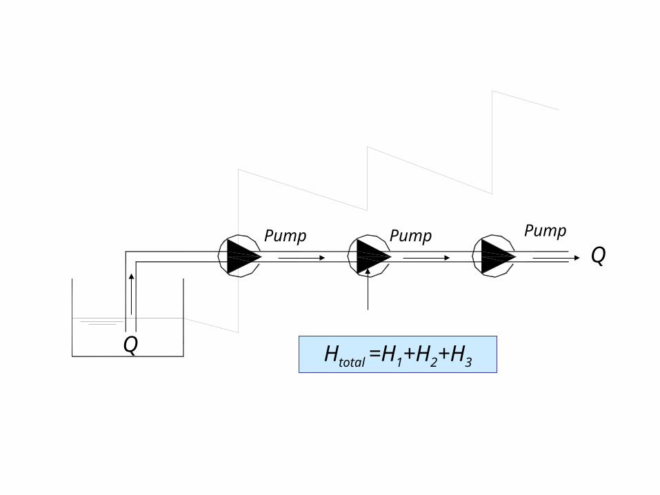
Q

Pump PumpPumpQ

Htotal =H1+H2+H3

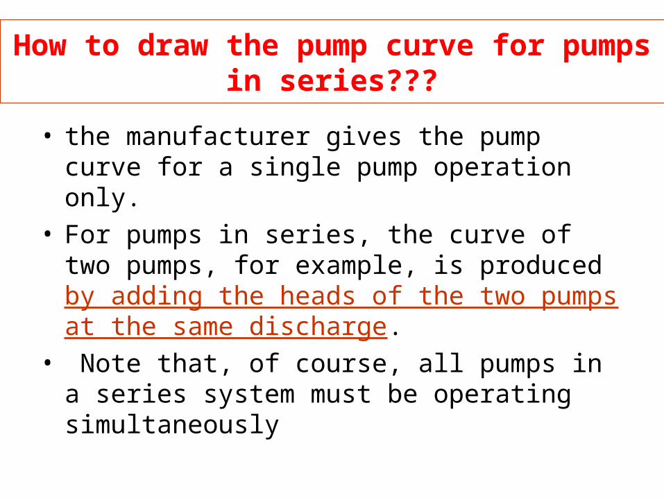
How to draw the pump curve for pumps in series???

• the manufacturer gives the pump curve for a single pump operation only.

• For pumps in series, the curve of two pumps, for example, is produced by adding the heads of the two pumps at the same discharge.

• Note that, of course, all pumps in a series system must be operating simultaneously

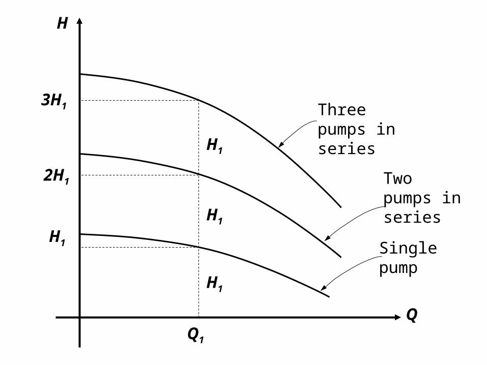
H

QQ1

H1

H1

H1

2H1

H1

3H1

Single pump

Two pumps in series

Three pumps in series

Constant- and Variable-Speed Pumps

• The speed of the pump is specified by the angular speed of the impeller which is measured in revolution per minutes (rpm).

• Based on this speed, N , pumps can be divided into two types:

• Constant-speed pumps• Variable-speed pumps

Constant-speed pumps

• For this type, the angular speed , N , is constant. • There is only one pump curve which represents the

performance of the pump

Variable-speed pumps

• For this type, the angular speed , N , is variable, i.e.; pump can operate at different speeds.

• The pump performance is presented by several pump curves, one for each speed

• Each curve is used to suit certain operating requirements of the system.

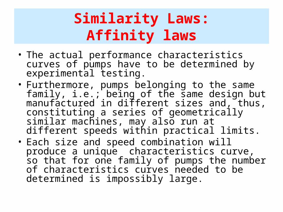
Similarity Laws:Affinity laws

• The actual performance characteristics curves of pumps have to be determined by experimental testing.

• Furthermore, pumps belonging to the same family, i.e.; being of the same design but manufactured in different sizes and, thus, constituting a series of geometrically similar machines, may also run at different speeds within practical limits.

• Each size and speed combination will produce a unique characteristics curve, so that for one family of pumps the number of characteristics curves needed to be determined is impossibly large.

• The problem is solved by the application of dimensional analysis and by replacing the variables by dimensionless groups so obtained. These dimensionless groups provide the similarity (affinity) laws governing the relationships between the variables within one family of geometrically similar pumps.

• Thus, the similarity laws enable us to obtain a set of characteristic curves for a pump from the known test data of a geometrically similar pump.

(a) Change in pump speed (constant size)

• If a pump delivers a discharge Q1 at a head H1 when running at speed N1, the corresponding values when the same pump is running at speed N2 are given by the similarity (affinity) laws:

QQ

NN

2

1

2

1 H

HNN

2

1

2

1

2

PP

NN

i

i

2

1

2

1

3

where Q = discharge (m3/s, or l/s).H = pump head (m).N = pump rotational speed (rpm).Pi = power input (HP, or kw).

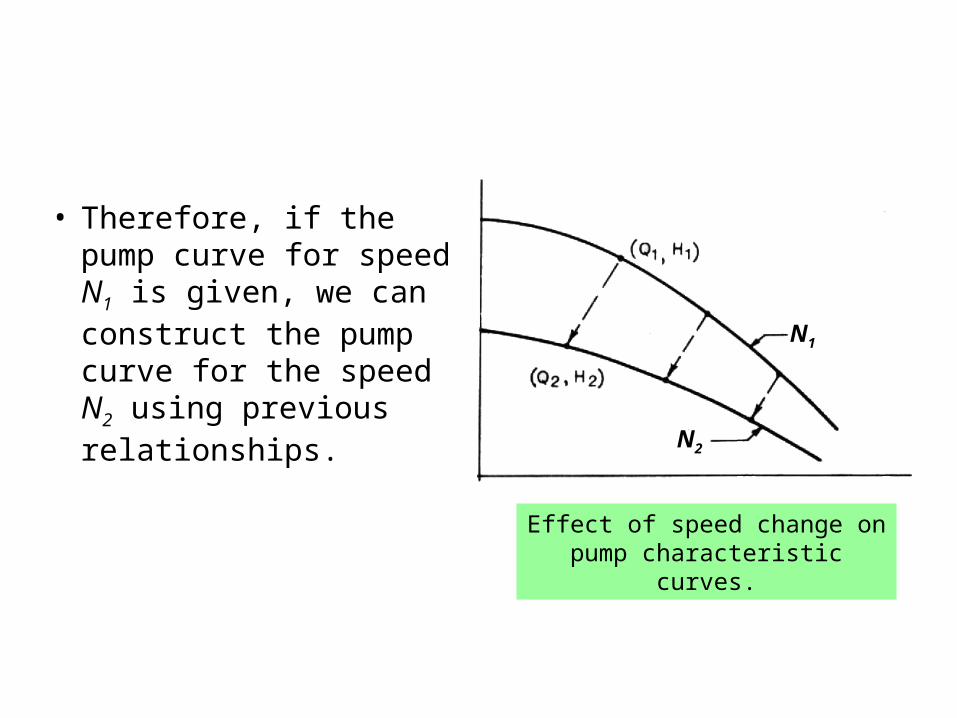
• Therefore, if the pump curve for speed N1 is given, we can construct the pump curve for the speed N2 using previous relationships.

Effect of speed change on pump characteristic curves.

N1

N2

(b) Change in pump size (constant speed)

• A change in pump size and therefore, impeller diameter (D), results in a new set of characteristic curves using the following similarity (affinity) laws:

QQ

DD

2

1

2

1

3

HH

DD

2

1

2

1

2

PP

DD

i

i

2

1

2

1

5

where D = impeller diameter (m, cm).

Note : D indicated the size of the pump

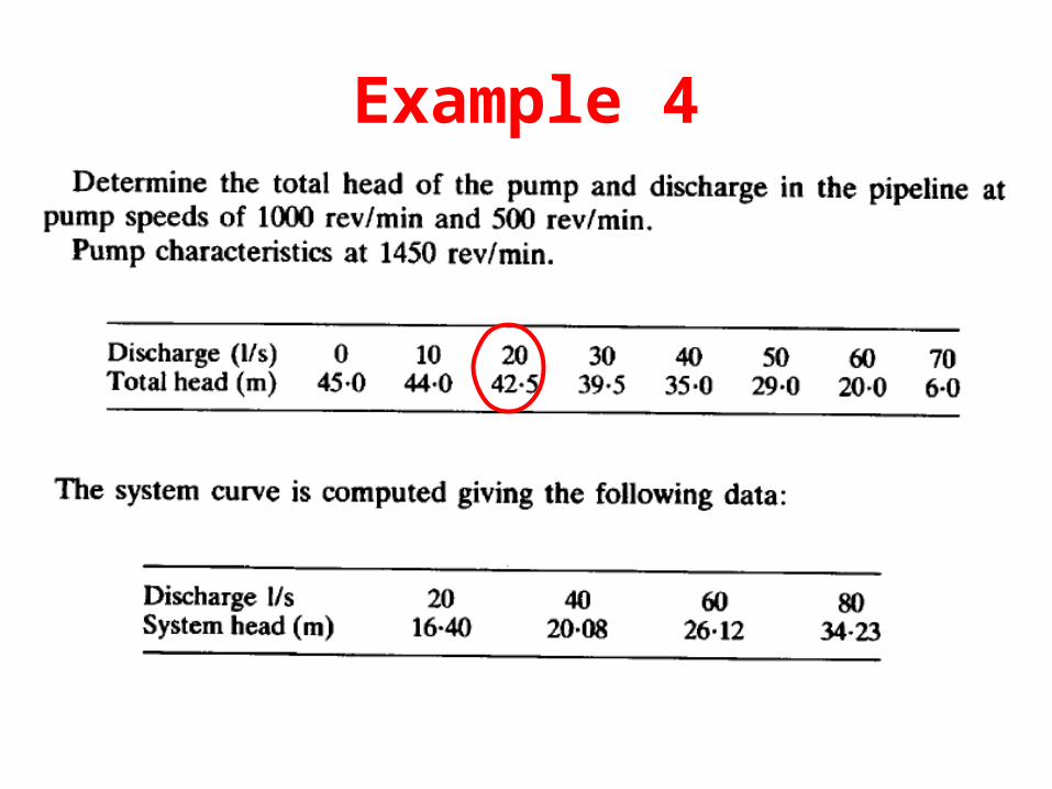
Example 4

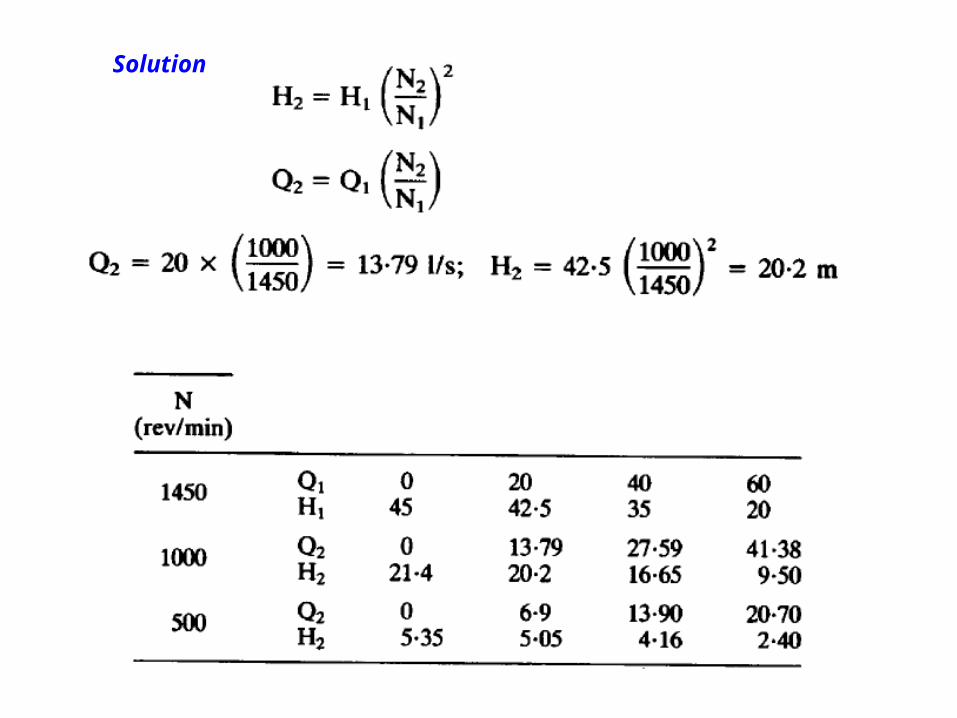
Solution

Specific Speed

• Pump types may be more explicitly defined by the parameter called specific speed (Ns) expressed by:

Where: Q = discharge (m3/s, or l/s).H = pump total head (m).N = rotational speed (rpm).

NN Q

Hs 3

4

• This expression is derived from dynamical similarity considerations and may be interpreted as the speed in rev/min at which a geometrically scaled model would have to operate to deliver unit discharge (1 l/s) when generating unit head (1 m).

• The given table shows the range of Ns values for the turbo-hydraulic pumps:

Pump type Ns range (Q - l/s, H-m)

centrifugal up to 2600mixed flow 2600 to 5000axial flow 5000 to 10 000

Example 5• A centrifugal pump running at 1000 rpm gave the following

relation between head and discharge:

Discharge (m3/min) 0 4.5 9.0 13.5 18.0 22.5

Head (m) 22.5 22.2 21.6 19.5 14.1 0

• The pump is connected to a 300 mm suction and delivery pipe the total length of which is 69 m and the discharge to atmosphere is 15 m above sump level. The entrance loss is equivalent to an additional 6m of pipe and f is assumed as 0.024.

1. Calculate the discharge in m3 per minute.2. If it is required to adjust the flow by regulating the pump

speed, estimate the speed to reduce the flow to one-half

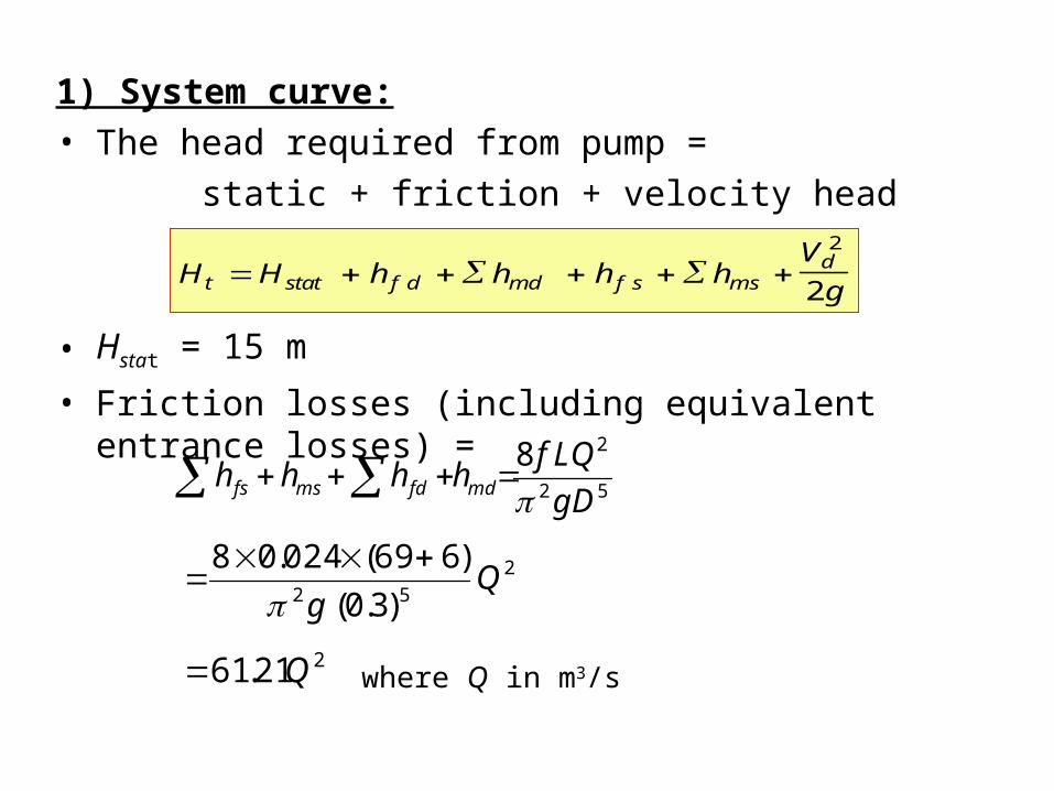
1) System curve:• The head required from pump = static + friction + velocity head

• Hstat = 15 m• Friction losses (including equivalent entrance losses) =

H H h h h hV

gt stat f d md f s msd 2

2

52

28DgQLfhhhh mdfdmsfs

252 )3.0(

)669(024.08Q

g

221.61 Q where Q in m3/s

• Velocity head in delivery pipe = where Q in m3/s Thus:• where Q in m3/sor • where Q in m3/min

• From this equation and the figures given in the problem the following table is compiled:

222

2.1021

2Q

AQ

ggVd

241.7115 QH t

231083.1915 QH t

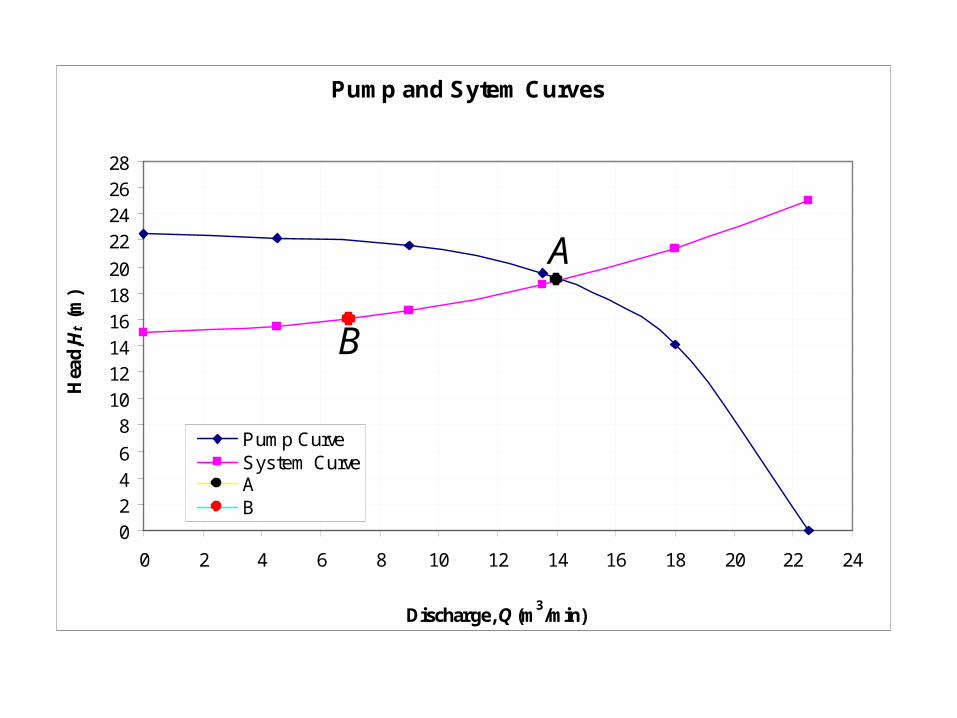
Discharge (m3/min) 0 4.5 9.0 13.5 18.0 22.5Head available (m) 22.5 22.2 21.6 19.5 14.1 0Head required (m) 15.0 15.4 16.6 18.6 21.4 25.0

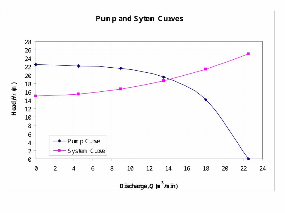
Pump and Sytem Curves

02468

10121416182022242628

0 2 4 6 8 10 12 14 16 18 20 22 24

Discharge, Q (m3/min)

Hea

d, H

t (m

)

Pump Curve

System Curve

From the previous Figure, The operating point is:• QA = 14 m3/min

• HA = 19 m

• At reduced speed: For half flow (Q = 7 m3/min) there will be a new operating point B at which:

• QB = 7 m3/min

• HB = 16 m• HomeWork How to estimate the new speed ?????

Pump and Sytem Curves

02468

10121416182022242628

0 2 4 6 8 10 12 14 16 18 20 22 24

Discharge, Q (m3/min)

Hea

d, H

t (m

)

Pump CurveSystem CurveAB

A

B

QQ

NN

2

1

2

1 H

HNN

2

1

2

1

2

2

BB QQ

HH

222 327.0

716 QQH

This curve intersects the original curve for N1 = 1000 rpm at C where Qc= 8.2 m3/ hr and Hc= 21.9 m, then

1

2

NN

QQ

C

B 10002.8

7 2N N2 = 855rpm

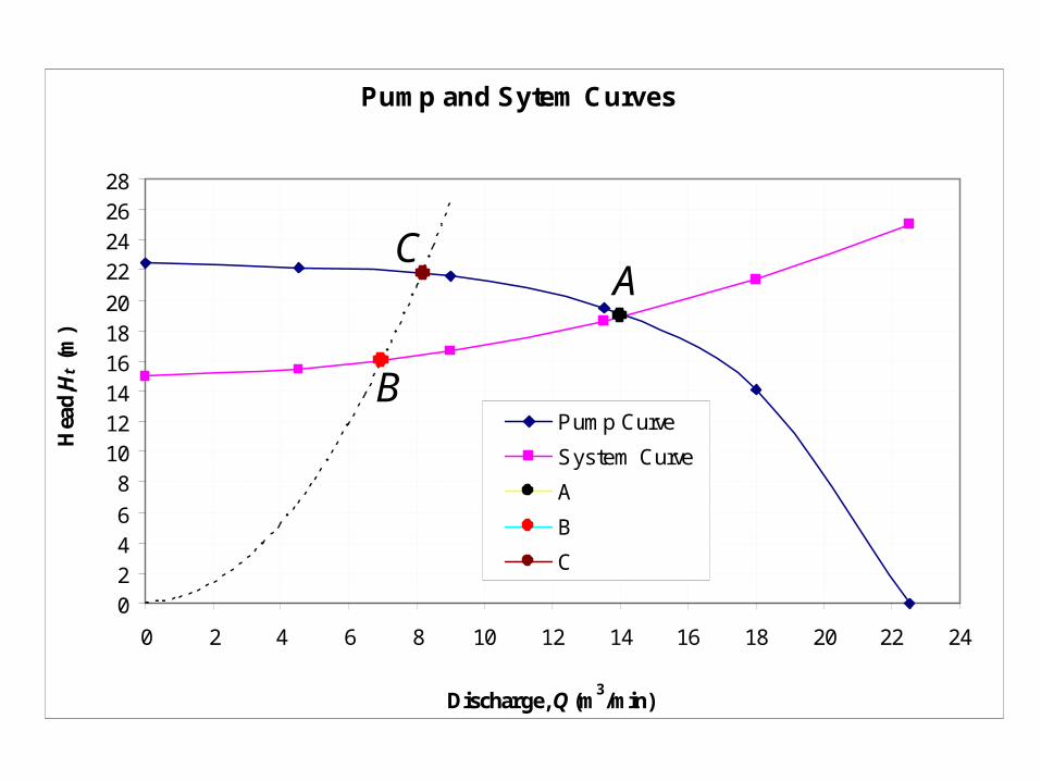
Pump and Sytem Curves

02468

10121416182022242628

0 2 4 6 8 10 12 14 16 18 20 22 24

Discharge, Q (m3/min)

Hea

d, H

t (m

)

Pump Curve

System Curve

A

B

C

A

B

C

Example 6

Abbreviations: G.V = Gate ValveC.V = Check ValveA.V = Air release ValveE.R = Eccentric ReducerC.I = Concentric increaseI.N = Inlet NozzleO.N = Outlet NozzleS.P = Suction PipeD.P = Delivery PipeW.W = Wet Well D.W = Dry Well

Data:

1. Flow rates and dimensions:Qmax = 0.05 m3/s Qmin = 0.025 m3/s LS.P = 5.0 m LD.P = 513.5 mDS.P = 250mm DD.P = 200mmHstat = 5.3 m, hS = 3.0 m

2. Minor Losses Coefficients (k):

G.V = 0.1 C.V = 2.5 A.V = 0.05,E.R = 0.1 C.I = 0.05 Elbow = 0.2 Bends in D.P = 0.05,Entrance of S.P = 0.3 (bell mouth)

3. Coefficient of friction: f = 0.02 (assumed constant).

I N O N mm. . 150

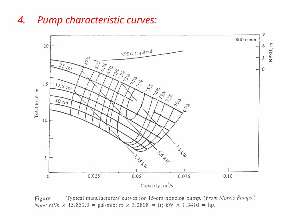
4. Pump characteristic curves:

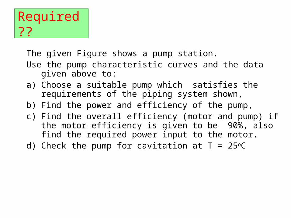
Required??

The given Figure shows a pump station. Use the pump characteristic curves and the data given above to:a) Choose a suitable pump which satisfies the requirements of

the piping system shown,b) Find the power and efficiency of the pump,c) Find the overall efficiency (motor and pump) if the motor

efficiency is given to be 90%, also find the required power input to the motor.

d) Check the pump for cavitation at T = 25oC

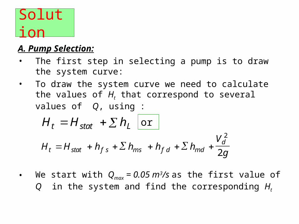
Solution

A. Pump Selection:• The first step in selecting a pump is to draw the system

curve:• To draw the system curve we need to calculate the values of

Ht that correspond to several values of Q, using :

• We start with Qmax = 0.05 m3/s as the first value of Q in the system and find the corresponding Ht

H H ht stat L or

H H h h h hV

gt stat f s m s f d mdd 2

2

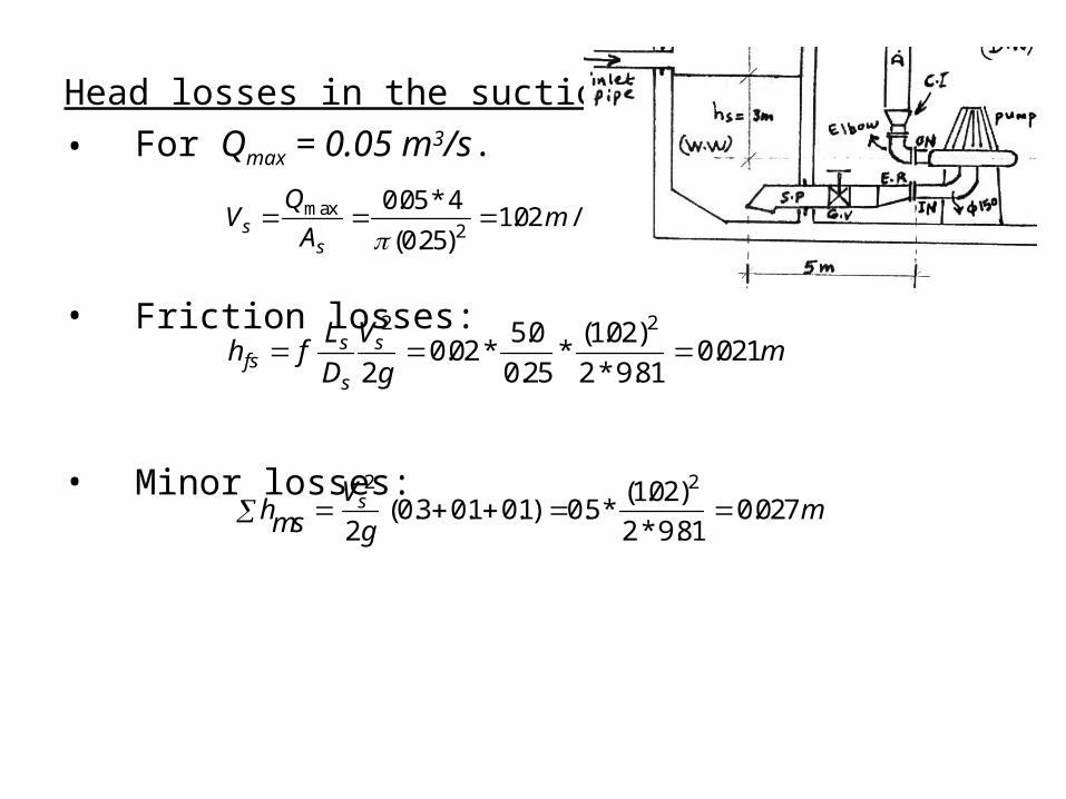
Head losses in the suction pipe:• For Qmax = 0.05 m3/s.

• Friction losses:

• Minor losses:

VQ

Am ss

s max . *

(0. ). /

0 05 425

1022

h fLD

Vg

mfss

s

s 2 2

20 02

5 00 25

1022 9 81

0 021. *..

*( . )

* ..

hmsV

gms

2 2

20 3 01 01 0 5

1022 9 81

0 027( . . . ) . *( . )

* ..

Head losses in the delivery pipe:• For Qmax = 0.05 m3/s.

• Friction losses:

• Minor losses:

VQ

Am sd

d max . *

( . ). /

0 05 40 20

162

h fLD

Vg

mfdd

d

d 2 2

20 02

51350 2

162 9 81

6 7. *.

.*

( . )* .

.

hmdV

gmd

2 2

20 2 0 05 0 2 0 05 2 5 01 2 0 05 32

162 9 81

0 42( . . . . . . * . ) . *( . )* .

.

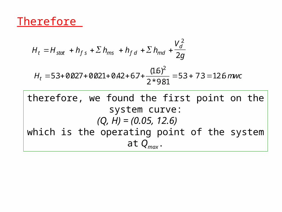
Therefore

H mwct 5 3 0 027 0 021 0 42 6 716

2 9 815 3 7 3 12 6

2. . . . .

( . )* .

. . .

H H h h h hV

gt stat f s m s f d mdd 2

2

therefore, we found the first point on the system curve:(Q, H) = (0.05, 12.6)

which is the operating point of the system at Qmax.

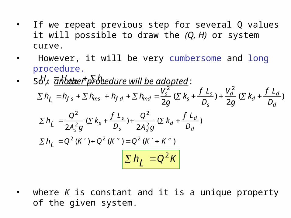
• If we repeat previous step for several Q values it will possible to draw the (Q, H) or system curve.

• However, it will be very cumbersome and long procedure. • So, another procedure will be adopted:

• where K is constant and it is a unique property of the given system.

H H ht stat L

hL h h h hV

gk

f LD

Vg

kf LDf s m s f d md

ss

s

s

dd

d

d

2 2

2 2( ) ( )

hLQA g

kf LD

QA g

kf LDs

ss

s dd

d

d

2

2

2

22 2( ) ( )

hL Q K Q K Q K K 2 2 2( ) ( ) ( )

hL Q K 2

• Therefore

• Thus:

)2.435.51(2

)5.04(2 2

2

2

2

gA

QgA

QLh

ds

22 64.51)2.435.51(15.21)5.04( QQLh

288.2963 QLh

288.29633.5 QH t

• for a given Qi , we have

• for Qmax , we have

• Therefore

• Or

hLi Q Ki 2

hL Q Kmax max 2

hh

QQ

Li

L

i

max max

2

2

hQ

QhLi

iL

maxmax*

2

From previous calculations we obtained for Qmax = 0.05 m3/s. Therefore, we can use the above equation along with the above values to find for several values of Qi . In order to calculate Hti.

hL mwcmax . 7 3

hLi

System curve

Operating point

System curve

12.6

It is clear from the above figure that the required pump is the

35-cm impeller pump

Pump Power Input and Efficiency

• From the pump curve we can read Pi = 7.5 kw

• and hence

P kw HPi 7 57 5 10

74510

3.

. *

po

i

t

i

PP

Q HP

1000 9 81 0 05 12 60

7 5 10006187 6

0824 82%* . * . * .

. *..

.

Overall Efficiency and Motor Power Input

• Overall efficiency

• and hence

o p m 0 9 0 82 0 738 738. * . . . %

oo

m m

PP P

618

0 738.

.

P kw HPm 8 27 11 2. .

Check for Cavitation:• To prevent cavitation we must have:

(NPSH)A (NPSH)R

• From pump curve figure we can read:(NPSH)R = 3 m at Qmax = 0.05 m3/s.

• For water at T=25oC, Patm= 101 kN/m2, and Pvapor = 3.17 kN/m2.

• Using the equation

• we can write

• no cavitation.

( )NPSHP

h h hP

Aatm

s f s m svapor

( )** .

. .. *

* .NPSH A

101 10001000 9 81

3 0 021 0 027317 10001000 9 81

( ) .NPSH m mA 12 924 3

Home Work