chapter 4 derivative-free optimization - stanford...

Chapter 4Derivative-Free Optimization

Oliver Kramer, David Echeverrıa Ciaurri, and Slawomir Koziel

Abstract. In many engineering applications it is common to find optimizationproblems where the cost function and/or constraints require complex simulations.Though it is often, but not always, theoretically possible in these cases to ex-tract derivative information efficiently, the associated implementation proceduresare typically non-trivial and time-consuming (e.g., adjoint-based methodologies).Derivative-free (non-invasive, black-box) optimization has lately received consid-erable attention within the optimization community, including the establishment ofsolid mathematical foundations for many of the methods considered in practice. Inthis chapter we will describe some of the most conspicuous derivative-free optimiza-tion techniques. Our depiction will concentrate first on local optimization such aspattern search techniques, and other methods based on interpolation/approximation.Then, we will survey a number of global search methodologies, and finally giveguidelines on constraint handling approaches.

4.1 Introduction

Efficient optimization very often hinges on the use of derivative information ofthe cost function and/or constraints with respect to the design variables. In the last

Oliver KramerUC Berkeley, Berkeley, CA 94704, USAe-mail: [email protected]

David Echeverrıa CiaurriDepartment of Energy Resources Engineering,Stanford University, Stanford, CA 94305-2220, USAe-mail: [email protected]

Slawomir KozielEngineering Optimization & Modeling Center,School of Science and Engineering, Reykjavik University, Menntavegur 1,101 Reykjavik, Icelande-mail: [email protected]

S. Koziel & X.-S. Yang (Eds.): Comput. Optimization, Methods and Algorithms, SCI 356, pp. 61–83.springerlink.com c© Springer-Verlag Berlin Heidelberg 2011

[email protected]

[email protected]

[email protected]

62 O. Kramer, D. Echeverrıa Ciaurri, and S. Koziel

decades, the computational models used in design have increased in sophisticationto such an extent that it is common to find situations where (reliable) derivativeinformation is not available. Although in simulation-based design there are method-ologies that allow one to extract derivatives with a modest amount of additional com-putation, these approaches are in general invasive with respect to the simulator (e.g.,adjoint-based techniques [1]), and thus, require precise knowledge of the simulationcode and access to it. Moreover, obtaining derivatives in this intrusive way oftenimplies significant coding (not only at the code development stage, but also sub-sequently, when maintaining or upgrading the software), and consequently, manysimulators simply yield, as output, the data needed for the cost function and/or con-straint values. Furthermore, optimal design has currently a clear multidisciplinarynature, so it is reasonable to expect that some components of the overall simula-tion do not include derivatives. This situation is even more likely when commercialsoftware is used, since then the source code is typically simply inaccessible.

In this chapter we review a number of techniques that can be applied to gener-ally constrained continuous optimization problems for which the cost function andconstraint computation can be considered as a black box system. We wish to clearlydistinguish between methods that aim at providing just a solution (local optimiza-tion; see Section 4.3), and approaches that try to avoid being trapped in local optima(global optimization; see Section 4.4). Local optimization is much easier to handlethan global optimization, since, in general, there is no algorithmically suitable char-acterization of global optima. As a consequence, there are more theoretical results ofpractical relevance for local than for global optimizers (e.g., convergence conditionsand rate). For more details on theoretical aspects of derivative-free optimization westrongly recommend both the review [2] and the book [3]. The techniques are de-scribed for continuous variables, but it is possible to apply, with care, extensions ofmany of them to mixed-integer scenarios. However, since mixed-integer nonlinearprogramming is still an emergent area (especially in simulated-based optimization),we prefer not to include recommendations in this case.

In some situations, numerical derivatives can be computed fairly efficiently (e.g.,via a computer cluster), and still yield results that can be acceptable in practice.However, if the function/constraint evaluations are even moderately noisy, numer-ical derivatives are usually not useful. Though methods that rely on approximatederivatives are not derivative-free techniques per se, for example, in the absence ofnoise, they can address optimization in a black box approach. We should note thatin addition to their inherent additional computational costs, numerical derivativesvery often imply the tuning of the derivative approximation together with the sim-ulation tolerances, and this is not always easy to do. Implicit filtering [4, 5] maysomehow alleviate some of these issues. This approach is essentially a gradient-based procedure where the derivative approximation is improved as the optimizationprogresses. Implicit filtering has been recommended for problems with multiple lo-cal optima (e.g., noisy cost functions). For more details on gradient-based method-ologies the reader is encouraged to regard nonlinear optimization references (forexample, [6, 7]).

4 Derivative-Free Optimization 63

Many derivative-free methods are easy to implement, and this feature makes themattractive when approximate solutions are required in a short time frame. An obvi-ous statement that is often neglected is that the computational cost of an iterationof an algorithm is not always a good estimate of the time needed within a project(measured from its inception) to obtain results that are satisfactory. However, oneimportant drawback of derivative-free techniques (when compared, for example,with adjoint-based approaches) is the limitation on the number of optimization vari-ables that can be handled. For example, in [3] and [2] the limit given is a few hundredvariables. However, this limit in the problem size can be overcome, at least to someextent, if one is not restricted to a single sequential environment. For some of thealgorithms though, adequately exploiting parallelism may be difficult or even im-possible. When distributed computing resources are scarce or not available, and forsimulation-based designs with significantly more than a hundred optimization vari-ables, some form of parameter reduction is mandatory. In these cases, surrogatesor reduced order models [8] for the cost function and constraints are desirable ap-proaches. Fortunately, suitable parameter and model order reduction techniques canoften be found in many engineering applications, although they may give rise to in-accurate models. We should add that even in theory, as long as a problem with nons-mooth/noisy cost functions/constraints can be reasonably approximated by a smoothfunction (see [9], Section 10.6), some derivative-free optimization algorithms per-form well with nonsmooth/noisy cost functions, as has been observed in practice[2, 3].

In the last decade, there has been a renaissance of gradient-free optimizationmethodologies, and they have been successfully applied in a number of areas. Exam-ples of this are ubiquitous; to name a few, derivative-free techniques have been usedwithin molecular geometry [10], aircraft design [11, 12], hydrodynamics [13, 14],medicine [15, 16] and earth sciences [17, 18, 19, 20]. These references includegenerally constrained cases with derivative-free objective functions and constraints,continuous and integer optimization variables, and local and global approaches. Inspite of all this apparent abundance of results, we should not disregard the generalrecommendation (see [3, 2]) of strongly preferring gradient-based methods if accu-rate derivative information can be computed reasonably efficiently and globally.

This chapter is structured as follows. In Section 4.2 we introduce the gen-eral problem formulation and notation. A number of derivative-free methodologiesfor unconstrained continuous optimization are presented in the next two sections.Section 4.3 refers to local optimization, and Section 4.4 is devoted to global op-timization. Guidelines for extending all these algorithms to generally constrainedoptimization are given in Section 4.5. We bring the chapter to an end with someconclusions and recommendations.

4.2 Derivative-Free Optimization

A general single-objective optimization problem can be formally stated as:

minx∈Ω⊂Rn

f (x) subject to g(x) ≤ 0, (4.1)


where f (x) is the objective function, x ∈ Rn is the vector of control variables, and

g : Rn → R

m represents the nonlinear constraints in the problem. Bound and linearconstraints are included in the set Ω ⊂R

n. For many approaches it is natural to treatany constraints for which derivatives are available separately. In particular, boundsand linear constraints, and any other structure than can be exploited, should be. Sofor example, nonlinear least-squares problems should exploit that inherent structurewhenever possible (see e.g. [21]). We are interested in applications for which theobjective function and constraint variables are computed using the output from asimulator, rendering function evaluations expensive and derivatives unavailable.

We will begin by discussing some general issues with respect to optimizationwith derivatives since they have important relevancy to the derivative-free case.Essentially all approaches to the former are somewhere between steepest descentand Newton’s method, or equivalently use something that is between a linear anda quadratic model. This is reinforced by the realization that almost all practicalcomputation is linear at its core, and (unconstrained) minima are characterized bythe gradient being zero, and quadratic models give rise to linear gradients. In fact,theoretically at least, steepest descent is robust but slow (and in fact sometimes soslow that in practice it is not robust) whereas Newton’s method is fast but may havea very small radius of convergence. That is, one needs to start close to the solu-tion. It is also computationally more demanding. Thus in a sense, most practicalunconstrained algorithms are intelligent compromises between these two extremes.Although, somewhat oversimplified, one can say that the constrained case is dealtwith by being feasible, determining which constraints are tight, linearizing theseconstraints and then solving the reduced problem determined by these linearizations.Therefore, some reliable first-order model is essential, and for faster convergence,something more like a second-order model is desirable. In the unconstrained casewith derivatives these are typically provided by a truncated Taylor series model (inthe first-order case) and some approximation to a truncated second-order Taylor se-ries model. A critical property of such models is that as the step sizes become smallthe models become more accurate. In the case where derivatives, or good approx-imations to them, are not available, clearly, one cannot use truncated Taylor seriesmodels. It thus transpires that, if for example, one uses interpolation or regressionmodels, that depend only on function values, one can no longer guarantee that as thestep sizes become small the models become more accurate. Thus one has to havesome explicit way to make this guarantee, at least approximately. It turns out thatthis is usually done by considering the geometry of the points at which the func-tion is evaluated, at least, before attempting to decrease the effective maximum stepsize. In pattern search methods, this is done by explicitly using a pattern with goodgeometry, for example, a regular mesh that one only scales while maintaining the apriori good geometry.

In the derivative case the usual stopping criteria relates to the first-order optimal-ity conditions. In the derivative-free case, one does not explicitly have these, sincethey require (approximations to) the derivatives. At this stage we just remark thatany criteria used should relate to the derivative case conditions, so, for example oneneeds something like a reasonable first-order model, at least asymptotically.


4.3 Local Optimization

The kernel of many optimizers are local methods. This is not surprising, since, aswe already mentioned, there is no suitable algorithmic characterization of globaloptima unless one considers special situations such as where all local optima areglobal, as for example in convex minimization problems. In this section we con-centrate on local search methods based on pattern search and also on interpolationand approximation models. Some constraint handling procedures are described inSection 4.5.

4.3.1 Pattern Search Methods

Pattern search methods are optimization procedures that evaluate the cost functionin a stencil-based fashion determined by a set of directions with intrinsic prop-erties meant to be desirable from a geometric/algebraic point of view. This sten-cil is sequentially modified as iterations proceed. The recent popularity of theseschemes is due in part to the development of a mathematically sound convergencetheory [2, 3]. Moreover, they are attractive because they can relatively easily lever-age the widespread availability of parallel computing resources. However, mostpublished computational results are not parallel exploiting.

4.3.1.1 Generalized Pattern Search

Generalized pattern search (GPS; [22, 23]) refers to a whole family of optimiza-tion methods. GPS relies on polling (local exploration of the cost function on thepattern) but may be enhanced by additional searches, see [23]. At any particular it-eration a stencil (pattern) is centered at the current solution. The stencil comprisesa set of directions such that at least one direction is a descent direction. This is alsocalled a generating set (see e.g. [2]). If any of the points in the stencil represent animprovement in the cost function, the stencil is moved to one of them. Otherwise,the stencil size is decreased. The optimization progresses until some stopping crite-rion is satisfied (typically, a minimum stencil size). Generalized pattern search canbe further generalized by polling in an asymptotically dense set of directions (thisset varies with the iterations). The resulting algorithm is the mesh adaptive directsearch (MADS; [24]). In particular, some generalization of a simple fixed pattern isessential for constrained problems. The GPS method parallelizes naturally since, at aparticular iteration, the objective function evaluations at the polling points can be ac-complished in a distributed fashion. The method typically requires on the order of nfunction evaluations per iteration (where n is the number of optimization variables).

4.3.1.2 Hooke-Jeeves Direct Search

The Hooke-Jeeves direct search (HJDS; [25]) is another pattern search method andwas the first to use the term ‘direct search’ method and take advantage of the idea


optimum

Exploratory movePattern moveImprovementNo Improvement

x

x

x

0

1

2

d

d

1

2

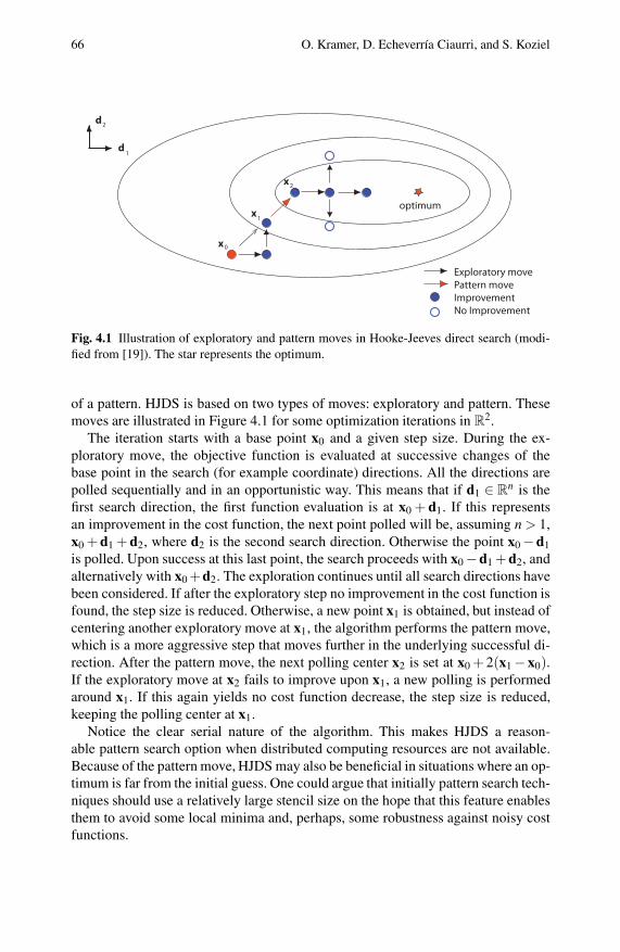
Fig. 4.1 Illustration of exploratory and pattern moves in Hooke-Jeeves direct search (modi-fied from [19]). The star represents the optimum.

of a pattern. HJDS is based on two types of moves: exploratory and pattern. Thesemoves are illustrated in Figure 4.1 for some optimization iterations in R

2.The iteration starts with a base point x0 and a given step size. During the ex-

ploratory move, the objective function is evaluated at successive changes of thebase point in the search (for example coordinate) directions. All the directions arepolled sequentially and in an opportunistic way. This means that if d1 ∈ R

n is thefirst search direction, the first function evaluation is at x0 + d1. If this representsan improvement in the cost function, the next point polled will be, assuming n > 1,x0 + d1 + d2, where d2 is the second search direction. Otherwise the point x0 −d1

is polled. Upon success at this last point, the search proceeds with x0 −d1 + d2, andalternatively with x0 +d2. The exploration continues until all search directions havebeen considered. If after the exploratory step no improvement in the cost function isfound, the step size is reduced. Otherwise, a new point x1 is obtained, but instead ofcentering another exploratory move at x1, the algorithm performs the pattern move,which is a more aggressive step that moves further in the underlying successful di-rection. After the pattern move, the next polling center x2 is set at x0 + 2(x1 −x0).If the exploratory move at x2 fails to improve upon x1, a new polling is performedaround x1. If this again yields no cost function decrease, the step size is reduced,keeping the polling center at x1.

Notice the clear serial nature of the algorithm. This makes HJDS a reason-able pattern search option when distributed computing resources are not available.Because of the pattern move, HJDS may also be beneficial in situations where an op-timum is far from the initial guess. One could argue that initially pattern search tech-niques should use a relatively large stencil size on the hope that this feature enablesthem to avoid some local minima and, perhaps, some robustness against noisy costfunctions.


4.3.2 Derivative-Free Optimization with Interpolation andApproximation Models

The other major approach to derivative-free optimization is based on building mod-els that are meant to approximate the functions and then make use of derivativemethods on the models. The advantage is that one is trying to take account of theshape of the function rather than naively just using the function evaluations alone.As our introductory remarks in Section 4.2 suggest we can expect our models to beat least first-order models or better still, second-order.

A major drawback of this approach is that, since the models are not based uponan a priori pattern, as with just polling, the geometry of the sample points used re-quires special attention. Additionally, one pays for the extra sophistication of thesemethods in that they are not obviously parallelizable. Some of the better known al-gorithms in this class include DFO [3], NEWUOA [26] and BOOSTERS [27]. Thebasic ideas will be given here but it is recommended that the diligent reader consultChapters 3-6 of [3].

First of all, what does good geometry mean? Essentially, for example, if onewants to consider interpolation by a polynomial of degree d, where d = 1, that islinear interpolation, one needs n + 1 points and good geometry means they do notlie on or close to a linear surface. Similarly, if one wants to consider interpolationby a polynomial of degree d, where d = 2, that is quadratic interpolation, one needs(n + 1)(n + 2)/2 points and good geometry means they do not lie on or close to aquadratic or linear surface. The extension to higher degree is clear. One can alsosee why the problem goes away if one works with a suitable pattern, as in a patternsearch method.

Now, all three methods mentioned above are trust-region based. For an in-troduction to trust-region techniques the readers are referred to [7], or [9] for amonographic volume. In the case with derivatives the essential ingredients are thefollowing. Starting at a given point x0 one has a region about that point, coinedthe trust region and denoted by Δ0. The trust region is typically a sphere in theEuclidean or in the infinity norm. One then requires a model m(x) for the true ob-jective function that is relatively easy to minimize within the trust region (e.g., atruncated first-order Taylor series or an approximation to a truncated second-orderTaylor series, about the current point). A search direction from the current point isdetermined based upon the model and one (approximately) minimizes the modelwithin the trust region.

The trust region can be updated in the following manner. Suppose y1 is the ap-proximate minimizer of the model within the trust region Δ0. We then compare thepredicted reduction to truth in the sense that we consider

ρ =f (x0)− f (y1)

m(x0)−m(y1).


Then typically one assigns some updating strategy to the trust-region radius Δ0

like

Δ1 =

⎧⎨

⎩

2 ·Δ0, if ρ > 0.9 ,Δ0, if 0.1 ≤ ρ ≤ 0.9 ,0.5 ·Δ0 if ρ < 0.1 ,

where Δ1 denotes the updated radius. In the first two cases x1 = y1 and in the thirdcase x1 = x0.

Thus, although oversimplified, if we are using Taylor series approximations forour models, within the trust management scheme one can ensure convergence to asolution satisfying first-order optimality conditions [9]. Perhaps the most importantdifference once derivatives are not available is that we cannot take Taylor seriesmodels and so, in general, optimality can no longer be guaranteed. In fact, we haveto be sure that when we reduce the trust-region radius it is because of the problemand not just a consequence of having a bad model as a result of poor geometry ofthe sampling points. So it is here that one has to consider the geometry. Fortunately,it can be shown that one can constructively ensure good geometry, and with that,support the whole derivative-free approach with convergence to solutions that satisfyfirst-order optimality conditions. For details see [3], Chapter 6.

4.4 Global Optimization

In the previous section we have concentrated on local search methods. Unfortu-nately, most real-world problems are multimodal, and global optima are generallyextremely difficult to obtain. Local search methods find local optima that are notguaranteed to be global. Here we will give a short survey of global optimizationmethods. However, the reader should take note of the following. In practice, oftengood local optima suffice. If one is considering even a modest number of variables,say fifty, it is generally very difficult, if not impossible, to ensure convergence toa provable global solution, in a reasonable length of time, even if derivatives areavailable, not to mention in the derivative-free case. Almost all algorithms designedto determine local optima are significantly more efficient than global methods.

Many successful methods in global optimization are based on stochastic compo-nents, as they allow to escape from local optima and overcome premature stagnation.Famous classes of families of stochastic global optimization methods are evolution-ary algorithms, estimation of distribution algorithms, particle swarm optimization,and differential evolution. Further heuristics known in literature are simulated an-nealing [28, 29], tabu search [30, 31], ant colony optimization [32, 33], and artificialimmune systems [34, 35]. In this section, we concentrate on the first four classes ofmethods that have been successful in a number of practical applications.

4.4.1 Evolutionary Algorithms

A history of more than forty years of active research on evolutionary compu-tation indicates that stochastic optimization algorithms are an important class of


1 Start2 Initialize solutions xi of population P3 Evaluate objective function for the solutions xi in P4 Repeat5 For i = 0 To λ6 Select ρ parents from P7 Create new xi by recombination8 Mutate xi9 Evaluate objective function for xi10 Add xi to P ′11 Next12 Select μ parents from P ′ and form new P13 Until termination condition14 End

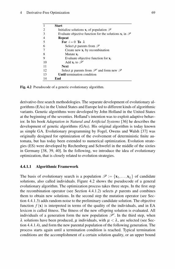
Fig. 4.2 Pseudocode of a generic evolutionary algorithm.

derivative-free search methodologies. The separate development of evolutionary al-gorithms (EAs) in the United States and Europe led to different kinds of algorithmicvariants. Genetic algorithms were developed by John Holland in the United Statesat the beginning of the seventies. Holland’s intention was to exploit adaptive behav-ior. In his book Adaptation in Natural and Artificial Systems [36] he describes thedevelopment of genetic algorithms (GAs). His original algorithm is today knownas simple GA. Evolutionary programming by Fogel, Owens and Walsh [37] wasoriginally designed for optimization of the evolvement of deterministic finite au-tomata, but has today been extended to numerical optimization. Evolution strate-gies (ES) were developed by Rechenberg and Schwefel in the middle of the sixtiesin Germany [38, 39, 40]. In the following, we introduce the idea of evolutionaryoptimization, that is closely related to evolution strategies.

4.4.1.1 Algorithmic Framework

The basis of evolutionary search is a population P := {x1, . . . ,xλ} of candidatesolutions, also called individuals. Figure 4.2 shows the pseudocode of a generalevolutionary algorithm. The optimization process takes three steps. In the first stepthe recombination operator (see Section 4.4.1.2) selects ρ parents and combinesthem to obtain new solutions. In the second step the mutation operator (see Sec-tion 4.4.1.3) adds random noise to the preliminary candidate solution. The objectivefunction f (x) is interpreted in terms of the quality of the individuals, and in EAlexicon is called fitness. The fitness of the new offspring solution is evaluated. Allindividuals of a generation form the new population P ′. In the third step, whenλ solutions have been produced, μ individuals, with μ < λ , are selected (see Sec-tion 4.4.1.4), and form the new parental population of the following generation. Theprocess starts again until a termination condition is reached. Typical terminationconditions are the accomplishment of a certain solution quality, or an upper bound


on the number of generations. We now concentrate on the stochastic operators thatare often used in evolutionary computation.

4.4.1.2 Recombination

In biological systems recombination, also known as crossover, mixes the geneticmaterial of two parents. Most EAs also make use of a recombination operator andcombine the information of two or more individuals into a new offspring solution.Hence, the offspring carries parts of the genetic material of its parents. The use ofrecombination is discussed controversially within the building block hypothesis byGoldberg [41, 42], and the genetic repair effect by Beyer [43].

Typical recombination operators for continuous representations are dominantand intermediary recombination. Dominant recombination randomly combines thegenes of all parents. If we consider parents of the form x = (x1, . . .xn), dominant re-combination with ρ parents x1, . . . ,xρ creates the offspring vector x′ = (x′1, . . . ,x

′n)

by random choice of the i-th component x′i:

x′i := xki , k ∈ random {1, . . . ,ρ}. (4.2)

Intermediate recombination is appropriate for integer and real-valued solutionspaces. Given ρ parents x1, . . . ,xρ each component of the offspring vector x′ isthe arithmetic mean of the components of all ρ parents. Thus, the characteristics ofdescendant solutions lie between their parents:

x′i :=1ρ

ρ

∑k=1

xki . (4.3)

Integer representations may require rounding procedures to produce intermediateinteger solutions.

4.4.1.3 Mutation

Mutation is the second main source for evolutionary changes. According to Beyerand Schwefel [38], a mutation operator is supposed to fulfill three conditions. First,from each point in the solution space each other point must be reachable. Second,in unconstrained solution spaces a bias is disadvantageous, because the direction tothe optimum is not known. And third, the mutation strength should be adjustablein order to adapt to solution space conditions. In the following, we concentrate onthe well-known Gaussian mutation operator. We assume that solutions are vectorsof real values. Random numbers based on the Gaussian distribution N (0,1) satisfythese conditions in continuous domains. The Gaussian distribution can be used todescribe many natural and artificial processes. By isotropic Gaussian mutation eachcomponent of x is perturbed independently with a random number from a Gaussiandistribution with zero mean and standard deviation σ .


x1

x2

x2

x2

x1

x1

isotropic multivariate correlated

Fig. 4.3 Gaussian mutation: isotropic Gaussian mutation (left) uses one step size σ for eachdimension, multivariate Gaussian mutation (middle) allows independent step sizes for eachdimension, and correlated mutation (right) introduces an additional rotation of the coordinatesystem

The standard deviation σ plays the role of the mutation strength, and is alsoknown as step size. The step size σ can be kept constant, but convergence can beimproved by adapting σ according to the local solution space characteristics. Incase of high success rates, i.e., a high number of offspring solutions being betterthan their parents, large step sizes are advantageous in order to promote the explo-ration of the search space. This is often the case at the beginning of the search.Small step sizes are appropriate for low success rates. This is frequently adequatein later phases of the search, when the optimization history can be exploited whilethe optimum is approximated. An example for an adaptive control of step sizes isthe 1/5-th success rule by Rechenberg [39] that increases the step size if the successrate is over 1/5-th, and decreases it, if the success rate is lower.

The isotropic Gaussian mutation can be extended to the multivariate Gaussianmutation by introducing a step size vector σ with independent step sizes σi. Fig-ure 4.3 illustrates the differences between isotropic Gaussian mutation (left) andthe multivariate Gaussian mutation (middle). The multivariate variant considers amutation ellipsoid that adapts flexibly to local solution space characteristics.

Even more flexibility can be obtained through the correlated mutation proposedby Schwefel [44] that aligns the coordinate system to the solution space charac-teristics. The mutation ellipsoid is rotated by means of an orthogonal matrix, andthis rotation can be modified along iterations. The rotated ellipsoid is also shown inFigure 4.3 (right). The covariance matrix adaptation evolution strategies (CMA-ES)and derivates [45, 46] are self-adapting control strategies based on an automaticalignment of the coordinate system.

4.4.1.4 Selection

The counterpart of the variation operators mutation and recombination is selection.Selection gives the evolutionary search a direction. Based on the fitness, a subset ofthe population is selected, while the rest is rejected. In EAs the selection operator


can be utilized at two points. Mating selection selects individuals for recombina-tion. Another popular selection operator is survivor selection, corresponding to theDarwinian principle of survival of the fittest. Only the individuals selected by sur-vivor selection are allowed to confer genetic material to the following generation.The elitist strategies plus and comma selection choose the μ best solutions and areusually applied for survivor selection. Plus selection selects the μ best solutionsfrom the union P ∪P ′ of the last parental population P and the current offspringpopulation P ′, and is denoted by (μ +λ )-EA. In contrast to plus selection, commaselection, which is denoted by (μ ,λ )-EA, selects exclusively from the offspringpopulation, neglecting the parental population − even if individuals have superiorfitness. Though disregarding these apparently promising solutions may seem to bedisadvantageous, this strategy that prefers the new population to the old populationcan be useful to avoid being trapped in unfavorable local optima.

The deterministic selection scheme described in the previous paragraph is a char-acteristic feature of ES. Most evolutionary algorithms use selection schemes con-taining random components. An example is fitness proportionate selection (alsocalled roulette-wheel selection) popular in the early days of genetic algorithms [41].Another example is tournament selection, a widely used selection scheme for EAs.Here, the candidate with the highest fitness out of a randomly chosen subset of thepopulation is selected to the new population. The stochastic-based selection schemespermit survival of not-so-fit individuals and thus helps with preventing prematureconvergence and preserving the genetic material that may come in handy at laterstages of the optimization process.

4.4.2 Estimation of Distribution Algorithms

Related to evolutionary algorithms are estimation of distribution algorithms (EDAs).They also operate with a set of candidate solutions. Similar to ES, a random set ofpoints is initially generated, and the objective function is computed for all thesepoints. The core of EDAs are successive steps where distributions of the best solu-tions within a population are estimated, and a new population is sampled accordingto the previous distribution estimation.

The principle has been extended in a number of different manners. Most EDAsmake use of parametric distributions, i.e., the parameters of distribution functionsare determined in the estimation step. The assumption of a Gaussian distributionis frequent in EDAs. EDAs may suffer from premature convergence. The weightedvariance estimator introduced in [47] has been observed to alleviate that conver-gence issue. Adaptive variance scaling [48], i.e., the variance can be increased ifgood solutions are found, otherwise it is decreased, has also been suggested to avoidearly stagnation. The sampling process can be enhanced by anticipated mean shift(AMS; [49]). In this approach, about two thirds of the population are sampled regu-larly, and the rest is shifted in the direction of a previously estimated gradient. If thisestimate is accurate, all the shifted individuals, together with part of the non-shifted


individuals, may survive, and the variance estimate in the direction of the gradientcould be larger than without AMS.

4.4.3 Particle Swarm Optimization

Similar to evolutionary algorithms, particle swarm optimization (PSO) is a pop-ulation approach with stochastic components. Introduced by Kennedy and Eber-hart [50], it is inspired by the movement of natural swarms and flocks. The algorithmutilizes particles with a position x that corresponds to the optimization variables, anda speed v which is similar to the mutation strength in evolutionary computation. Theprinciple of particle swarm optimization is based on the idea that the particles movein the solution space, influencing each other with stochastic changes, while previoussuccessful solutions act as attractors.

In each iteration the position of particle x is updated by adding the currentvelocity v

x′ := x + v . (4.4)

The velocity is updated as follows

v′ := v + c1r1(x∗p −x)+ c2r2(x∗s −x) , (4.5)

where x∗p and x∗s denote the best previous positions of the particle and of the swarm,respectively. The weights c1 and c2 are acceleration coefficients that determine thebias of the particle towards its own or the swarm history. The recommendation givenby Kennedy and Eberhart is to set both parameters to one. The stochastic compo-nents r1 and r2 are uniformly drawn from the interval [0,1], and can be used topromote the global exploration of the search space.

4.4.4 Differential Evolution

Another population-based optimization approach is differential evolution (DE),originally introduced by Storn and Price [51]. As the algorithms in the previousthree subsections, DE exploits a set of candidate solutions (agents in DE lexicon).New agents are allocated in the search space by combining the positions of other ex-isting agents. More specifically, an intermediate agent is generated from two agentsrandomly chosen from the current population. This temporary agent is then mixedwith a predetermined target agent. The new agent is accepted for the next generationif and only if it yields reduction in objective function.

The basic DE algorithm uses a random initialization. A new agent y = [y1, . . . ,yn]is created from the existing one x = [x1, . . . ,xn] as indicated below.

1. Three agents a = [a1, . . . ,an], b = [b1, . . . ,bn] and c = [c1, . . . ,cn] are randomlyextracted from the population (all distinct from each other and from x).

2. A position index p ∈ {1, . . . ,N} is determined randomly.


3. The position of the new agent y is computed by means of the following iterationover i ∈ {1, . . . ,n}:

i) select a random number ri ∈ (0,1) with uniform probability distribution;ii) if i = p or ri <CR let yi = ai +F(bi−ci), otherwise let yi = xi; here, F ∈ [0,2]

is the differential weight and CR ∈ [0,1] is the crossover probability, bothdefined by the user;

iii) if f (y) < f (x) then replace x by y; otherwise reject y and keep x.

Although DE resembles some other stochastic optimization techniques, unlike tra-ditional EAs, DE perturbs the solutions in the current generation vectors with scaleddifferences of two randomly selected agents. As a consequence, no separate prob-ability distribution has to be used, and thus the scheme presents some degree ofself-organization. Additionally, DE is simple to implement, uses very few con-trol parameters, and has been observed to perform satisfactorily in a number ofmulti-modal optimization problems [52].

4.5 Guidelines for Generally Constrained Optimization

We now describe nonlinear constraint handling techniques that can be combinedwith the optimization methods presented in Sections 4.3 and 4.4.

4.5.1 Penalty Functions

The penalty function method (cf. [7]) for general optimization constraints involvesmodifying the objective function with a penalty term that depends on the constraintviolation h : R

n → R. The original optimization problem in (4.1) is thus modified asfollows:

minx∈Ω⊂Rn

f (x)+ ρ h(x) , (4.6)

where ρ > 0 is a penalty parameter. The modified optimization problem may stillhave constraints that are straightforward to handle.

If the penalty parameter is iteratively increased (tending to infinity), the solutionof (4.6) converges to that of the original problem in (4.1). However, in certain cases,a finite (and fixed) value of the penalty parameter ρ also yields the correct solution(this is the so-called exact penalty; see [7]). For exact penalties, the modified costfunction is not smooth around the solution [7], and thus the corresponding optimiza-tion problem can be significantly more involved than that in (4.6). However, one canargue that in the derivative-free case exact penalty functions may in some cases beattractive. Common definitions of h(x), where I and J denote the indices that referto inequality and equality constraints, respectively, are

h(x) = 12

(

∑i∈I

max(0,gi(x))2 + ∑j∈J

g2i (x)

)


the quadratic penalty and

h(x) = ∑i∈I

max(0,gi(x))+ ∑j∈J

|gi(x)|

an exact penalty. It should be noticed that by these penalties, the search considersboth feasible and infeasible points. Those optimization methodologies where theoptimum can be approached from outside the feasible region are known as exteriormethods.

The log-barrier penalty (for inequality constraints)

h(x) = −∑i∈I

log(−gi(x))

has to be used with a decreasing penalty parameter (tending to zero). This type ofpenalty methods (also known as barrier methods) confines the optimization to thefeasible region of the search space. Interior methods aim at reaching the optimumfrom inside the feasible region.

In [53], non-quadratic penalties have been suggested for pattern search tech-niques. However, the optimizations presented in that work are somewhat simplerthan those found in many practical situations, so the recommendations given mightnot be generally applicable. In future research, it will be useful to explore furtherthe performance of different penalty functions in the context of simulation-basedoptimization.

4.5.2 Augmented Lagrangian Method

As mentioned above, in exterior penalty function methods, as ρ → ∞ the local mini-mum is approached from outside the feasible region. Not surprisingly, there is a wayto shift the feasible region so one is able to determine the local solution for a finitepenalty parameter. See, for example, [54, 55] for original references, and also [7],Chapter 17.

Augmented Lagrangian methods [56, 57] aim at minimizing, in the equalityconstraint case, the following extended cost function

minx∈Ω⊂Rn

f (x)+ 12 ρ ‖g(x)‖2

2 + λλλ T g(x) , (4.7)

where ρ > 0 is a penalty parameter, and λλλ ∈ Rm are Lagrange multipliers. This cost

function can indeed be interpreted as a quadratic penalty with the constraints shiftedby some constant term [56]. As in penalty methods, the penalty parameter and theLagrange multipliers are iteratively updated. It turns out that if one is sufficientlystationary for Equation (4.7), which is exactly when we have good approximationsfor the Lagrange multipliers, then λλλ can be updated via

λλλ + = λλλ + ρ g(x) , (4.8)


h max h

( h , f )k

l

f

k

lf k

F

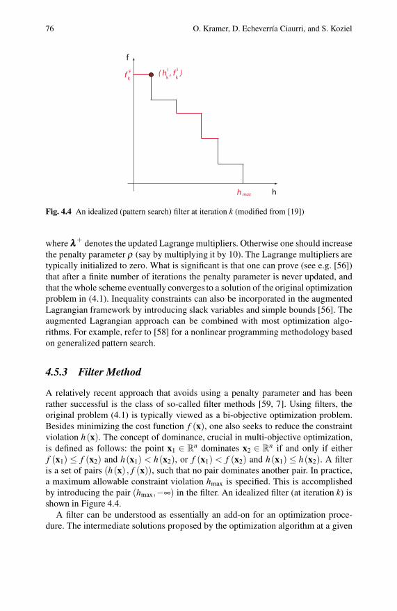
Fig. 4.4 An idealized (pattern search) filter at iteration k (modified from [19])

where λλλ + denotes the updated Lagrange multipliers. Otherwise one should increasethe penalty parameter ρ (say by multiplying it by 10). The Lagrange multipliers aretypically initialized to zero. What is significant is that one can prove (see e.g. [56])that after a finite number of iterations the penalty parameter is never updated, andthat the whole scheme eventually converges to a solution of the original optimizationproblem in (4.1). Inequality constraints can also be incorporated in the augmentedLagrangian framework by introducing slack variables and simple bounds [56]. Theaugmented Lagrangian approach can be combined with most optimization algo-rithms. For example, refer to [58] for a nonlinear programming methodology basedon generalized pattern search.

4.5.3 Filter Method

A relatively recent approach that avoids using a penalty parameter and has beenrather successful is the class of so-called filter methods [59, 7]. Using filters, theoriginal problem (4.1) is typically viewed as a bi-objective optimization problem.Besides minimizing the cost function f (x), one also seeks to reduce the constraintviolation h(x). The concept of dominance, crucial in multi-objective optimization,is defined as follows: the point x1 ∈ R

n dominates x2 ∈ Rn if and only if either

f (x1) ≤ f (x2) and h(x1) < h(x2), or f (x1) < f (x2) and h(x1) ≤ h(x2). A filteris a set of pairs (h(x) , f (x)), such that no pair dominates another pair. In practice,a maximum allowable constraint violation hmax is specified. This is accomplishedby introducing the pair (hmax,−∞) in the filter. An idealized filter (at iteration k) isshown in Figure 4.4.

A filter can be understood as essentially an add-on for an optimization proce-dure. The intermediate solutions proposed by the optimization algorithm at a given


iteration are accepted if they are not dominated by any point in the filter. The filteris updated at each iteration based on all the points evaluated by the optimizer. Wereiterate that, as for exterior methods, the optimization search is enriched by con-sidering infeasible points, although the ultimate solution is intended to be feasible(or very nearly so). Filters are often observed to lead to faster convergence thanmethods that rely only on feasible iterates.

Pattern search optimization techniques have been previously combined with fil-ters [60]. In Hooke-Jeeves direct search, the filter establishes the acceptance crite-rion for each (unique) new solution. For schemes where, in each iteration, multiplesolutions can be accepted by the filter (such as in GPS), the new polling center mustbe selected from the set of validated points. When the filter is not updated in a par-ticular iteration (and thus the best feasible point is not improved), the pattern size isdecreased. As in [60], when we combine GPS with a filter, the polling center at agiven iteration will be the feasible point with lowest cost function or, if no feasiblepoints remain, it will be the infeasible point with lowest constraint violation. Thesetwo points,

(0, f F

k

)and

(hI

k, f Ik

), respectively, are shown in Figure 4.4 (it is assumed

that both points have just been accepted by the filter, and thus it makes sense to useone of them as the new polling center). Refer to [60] and [61] for more details onpattern search filter methods.

4.5.4 Other Approaches

We will now briefly overview a number of constraint handling methodologies thathave been proposed for evolutionary algorithms. Repair algorithms [62, 63] projectinfeasible solutions back to the feasible space. This projection is in most cases ac-complished in an approximate manner, and can be as complex as solving the op-timization problem itself. Repair algorithms can be seen as local procedures thataim at reducing constraint violation. In the so-called Baldwinian case, the fitness ofthe repaired solution replaces the fitness of the original (infeasible) solution. In theLamarckian case, feasible solutions prevail over infeasible solutions.

Constraint-handling techniques borrowed from multi-objective optimization arebased on the idea of dealing with each constraint as an additional objective [64, 65,66, 67, 68, 69]. Under this assumption, multi-objective optimization methods suchas NSGA-II [70] or SPEA [71] can be applied. The output of a multi-objective ap-proach for constrained optimization is an approximation of a Pareto set that involvesthe objective function and the constraints. The user may then select one or more so-lutions from the Pareto set. A simpler but related and computationally less expensiveprocedure is the behavioral memory method presented in [72]. This evolutionarymethod concentrates on minimizing the constraint violation of each constraint se-quentially, and the objective function is addressed separately afterwards. However,treating objective function and constraints independently may yield in many casesinfeasible solutions.


Further constraint handling methods have been proposed in EA literature thatdo not rely either on repair algorithms or multi-objective approaches. In [73] atechnique based on a multi-membered evolution strategy with a feasibility compari-son mechanism is introduced. The dynamic multi-swarm particle optimizer studiedin [74] makes use of a set of sub-swarms that focus on different constraints, and iscoupled with a local search algorithm (sequential quadratic programming).

4.6 Concluding Remarks

In this chapter, we have concentrated on methods for solving optimization problemswithout derivates. The existence of local optima makes a hard optimization problemeven harder. Many methods have been proposed to solve non-convex optimizationproblems. The approaches range from pattern search for local optimization prob-lems to stochastic bio-inspired search heuristics for multi-modal problems. Deter-ministic local methods are guaranteed to find local optima, and restart variants canbe applied to avoid unsatisfactory solutions. Stochastic methods are not guaranteedto find the global optimum, but in some practical cases they can be beneficial.

The hybridization between local and global optimizers has led to a paradigmsometimes called memetic algorithms or hybrid metaheuristics [75, 76]. A numberof hybridizations have been proposed, but they are often tailored to specific prob-lem types and search domains due to their specific operators and methods. In thememetic method introduced in [77] for continuous search spaces, a gradient-basedscheme is combined with a deterministic perturbation component. The local opti-mization procedure for real-valued variables described in [78] is based on variableneighborhood search. It would be very useful if in future research some effort isdedicated to better understand from a theoretical point of view the hybridization oflocal and global optimization algorithms.

Most problems that can be found in practice present constraints. We have outlineda number of constraint handling techniques that can be incorporated in a derivative-free optimization framework. Though penalty functions are appealing due to theirsimplicity, some of the other approaches mentioned here may be more efficient andstill of a relatively easy implementation.

Multi-objective optimization is an important challenge for derivative-free method-ologies. Some of the evolutionary techniques mentioned above have performed suc-cessfully in some not especially involved multi-objective test cases. Other areaswhere derivative-free optimization could potentially be very helpful include dy-namic optimization, mixed-integer nonlinear programming, and optimization underuncertainty (stochastic programming).

Acknowledgements. We are grateful to the industry sponsors of the Stanford Smart FieldsConsortium for partial funding of this work, and also to J. Smith for his valuable suggestions.


References

[1] Pironneau, O.: On optimum design in fluid mechanics. Journal of Fluid Mechanics 64,97–110 (1974)

[2] Kolda, T.G., Lewis, R.M., Torczon, V.: Optimization by direct search: new perspec-tives on some classical and modern methods. SIAM Review 45(3), 385–482 (2003)

[3] Conn, A.R., Scheinberg, K., Vicente, L.N.: Introduction to Derivative-Free Optimiza-tion. MPS-SIAM Series on Optimization. MPS-SIAM (2009)

[4] Gilmore, P., Kelley, C.T.: An implicit filtering algorithm for optimization of functionswith many local minima. SIAM Journal on Optimization 5, 269–285 (1995)

[5] Kelley, C.T.: Iterative Methods for Optimization. In: Frontiers in Applied Mathemat-ics, SIAM, Philadelphia (1999)

[6] Dennis Jr., J.E., Schnabel, R.B.: Numerical Methods for Unconstrained Optimizationand Nonlinear Equations. SIAM’s Classics in Applied Mathematics Series. SIAM,Philadelphia (1996)

[7] Nocedal, J., Wright, S.J.: Numerical Optimization, 2nd edn. Springer, Heidelberg(2006)

[8] Schilders, W.H.A., van der Vorst, H.A., Rommes, J.: Model Order Reduction: The-ory, Research Aspects and Applications. Mathematics in Industry Series. Springer,Heidelberg (2008)

[9] Conn, A.R., Gould, N.I.M.: Toint, Ph.L.: Trust-Region Methods. MPS-SIAM Serieson Optimization. MPS-SIAM (2000)

[10] Meza, J.C., Martinez, M.L.: On the use of direct search methods for the molecularconformation problem. Journal of Computational Chemistry 15, 627–632 (1994)

[11] Booker, A.J., Dennis Jr., J.E., Frank, P.D., Moore, D.W., Serafini, D.B.: Optimizationusing surrogate objectives on a helicopter test example. In: Borggaard, J.T., Burns, J.,Cliff, E., Schreck, S. (eds.) Computational Methods for Optimal Design and Control,pp. 49–58. Birkhauser, Basel (1998)

[12] Marsden, A.L., Wang, M., Dennis Jr., J.E., Moin, P.: Trailing-edge noise reductionusing derivative-free optimization and large-eddy simulation. Journal of Fluid Me-chanics 572, 13–36 (2003)

[13] Duvigneau, R., Visonneau, M.: Hydrodynamic design using a derivative-free method.Structural and Multidisciplinary Optimization 28, 195–205 (2004)

[14] Fowler, K.R., Reese, J.P., Kees, C.E., Dennis Jr., J.E., Kelley, C.T., Miller, C.T., Audet,C., Booker, A.J., Couture, G., Darwin, R.W., Farthing, M.W., Finkel, D.E., Gablonsky,J.M., Gray, G., Kolda, T.G.: Comparison of derivative-free optimization methods forgroundwater supply and hydraulic capture community problems. Advances in WaterResources 31(5), 743–757 (2008)

[15] Oeuvray, R., Bierlaire, M.: A new derivative-free algorithm for the medical imageregistration problem. International Journal of Modelling and Simulation 27, 115–124(2007)

[16] Marsden, A.L., Feinstein, J.A., Taylor, C.A.: A computational framework forderivative-free optimization of cardiovascular geometries. Computational Methods inApplied Mechanics and Engineering 197, 1890–1905 (2008)

[17] Artus, V., Durlofsky, L.J., Onwunalu, J.E., Aziz, K.: Optimization of nonconven-tional wells under uncertainty using statistical proxies. Computational Geosciences 10,389–404 (2006)


[18] Dadashpour, M., Echeverrıa Ciaurri, D., Mukerji, T., Kleppe, J., Landrø, M.: Aderivative-free approach for the estimation of porosity and permeability using time-lapse seismic and production data. Journal of Geophysics and Engineering 7, 351–368(2010)

[19] Echeverrıa Ciaurri, D., Isebor, O.J., Durlofsky, L.J.: Application of derivativefreemethodologies for generally constrained oil production optimization problems. In-ternational Journal of Mathematical Modelling and Numerical Optimisation 2(2),134–161 (2011)

[20] Onwunalu, J.E., Durlofsky, L.J.: Application of a particle swarm optimization algo-rithm for determining optimum well location and type. Computational Geosciences 14,183–198 (2010)

[21] Zhang, H., Conn, A.R., Scheinberg, K.: A derivative-free algorithm for leastsquaresminimization. SIAM Journal on Optimization 20(6), 3555–3576 (2010)

[22] Torczon, V.: On the convergence of pattern search algorithms. SIAM Journal on Opti-mization 7(1), 1–25 (1997)

[23] Audet, C., Dennis Jr., J.E.: Analysis of generalized pattern searches. SIAM Journal onOptimization 13(3), 889–903 (2002)

[24] Audet, C., Dennis Jr., J.E.: Mesh adaptive direct search algorithms for constrainedoptimization. SIAM Journal on Optimization 17(1), 188–217 (2006)

[25] Hooke, R., Jeeves, T.A.: Direct search solution of numerical and statistical problems.Journal of the ACM 8(2), 212–229 (1961)

[26] Powell, M.J.D.: The NEWUOA software for unconstrained optimization withoutderivatives. Technical report DAMTP 2004/NA5, Dept. of Applied Mathematics andTheoretical Physics, University of Cambridge (2004)

[27] Oeuvray, R., Bierlaire, M.: BOOSTERS: a derivative-free algorithm based on radialbasis functions. International Journal of Modelling and Simulatio 29(1), 26–36 (2009)

[28] Metropolis, N., Rosenbluth, A., Teller, A., Teller, E.: Equation of state calculations byfast computing machines. Chemical Physics 21(6), 1087–1092 (1953)

[29] Kirkpatrick, S., Gelatt Jr., C.D., Vecchi, M.: Optimization by simulated annealing.Science 220(4498), 671–680 (1983)

[30] Glover, F.: Tabu search – part I. ORSA Journal on Computing 1(3), 190–206 (1990)[31] Glover, F.: Tabu search – part II. ORSA Journal on Computing 2(1), 4–32 (1990)[32] Dorigo, M.: Optimization, Learning and Natural Algorithms. PhD thesis, Dept. of

Electronics, Politecnico di Milano (1992)[33] Dorigo, M., Stutzle, T.: Ant Colony Optimization. Prentice-Hall, Englewood Cliffs

(2004)[34] Farmer, J., Packard, N., Perelson, A.: The immune system, adaptation and machine

learning. Physica 2, 187–204 (1986)[35] Castro, L.N.D., Timmis, J.: Artificial Immune Systems: A New Computational Intel-

ligence. Springer, Heidelberg (2002)[36] Holland, J.H.: Adaptation in Natural and Artificial Systems. University of Michigan

Press (1975)[37] Fogel, D.B.: Artificial Intelligence through Simulated Evolution. Wiley, Chichester

(1966)[38] Beyer, H.-G., Schwefel, H.-P.: Evolution strategies - a comprehensive introduction.

Natural Computing 1, 3–52 (2002)[39] Rechenberg, I.: Evolutionsstrategie: Optimierung Technischer Systeme nach Prinzip-

ien der Biologischen Evolution. Frommann-Holzboog (1973)


[40] Schwefel, H.-P.: Numerische Optimierung von Computer-Modellen mittel der Evolu-tionsstrategie. Birkhauser, Basel (1977)

[41] Goldberg, D.E.: Genetic Algorithms in Search, Optimization and Machine Learning.Addison-Wesley, Reading (1989)

[42] Holland, J.H.: Hidden Order: How Adaptation Builds Complexity. Addison- Wesley,London (1995)

[43] Beyer, H.-G.: An alternative explanation for the manner in which genetic algorithmsoperate. BioSystems 41(1), 1–15 (1997)

[44] Schwefel, H.-P.: Adaptive mechanismen in der biologischen evolution und ihr einflussauf die evolutionsgeschwindigkeit. In: Interner Bericht der Arbeitsgruppe Bionik undEvolutionstechnik am Institut fur Mess- und Regelungstechnik, TU Berlin (1974)

[45] Beyer, H.-G., Sendhoff, B.: Covariance matrix adaptation revisited – the CMSA evo-lution strategy –. In: Rudolph, G., Jansen, T., Lucas, S., Poloni, C., Beume, N. (eds.)PPSN 2008. LNCS, vol. 5199, pp. 123–132. Springer, Heidelberg (2008)

[46] Ostermeier, A., Gawelczyk, A., Hansen, N.: A derandomized approach to selfadapta-tion of evolution strategies. Evolutionary Computation 2(4), 369–380 (1994)

[47] Teytaud, F., Teytaud, O.: Why one must use reweighting in estimation of distributional-gorithms. In: Proceedings of the 11th Annual conference on Genetic and EvolutionaryComputation (GECCO 2009), pp. 453–460 (2009)

[48] Grahl, J., Bosman, P.A.N., Rothlauf, F.: The correlation-triggered adaptive variancescaling idea. In: Proceedings of the 8th Annual conference on Genetic and Evolution-ary Computation (GECCO 2006), pp. 397–404 (2006)

[49] Bosman, P.A.N., Grahl, J., Thierens, D.: Enhancing the performance of maximum–likelihood gaussian eDAs using anticipated mean shift. In: Rudolph, G., Jansen, T.,Lucas, S., Poloni, C., Beume, N. (eds.) PPSN 2008. LNCS, vol. 5199, pp. 133–143.Springer, Heidelberg (2008)

[50] Kennedy, J., Eberhart, R.: Particle swarm optimization. In: Proceedings of the IEEEInternational Conference on Neural Networks, pp. 1942–1948 (1995)

[51] Storn, R., Price, K.: Differential evolution - a simple and efficient heuristic for globaloptimization over continuous spaces. Journal of Global Optimization 11, 341–359(1997)

[52] Chakraborty, U.: Advances in Differential Evolution. SCI. Springer, Heidelberg (2008)[53] Griffin, J.D., Kolda, T.G.: Nonlinearly-constrained optimization using asynchronous

parallel generating set search. Technical report SAND2007-3257, Sandia NationalLaboratories (2007)

[54] Hestenes, M.R.: Multiplier and gradients methods. Journal of Optimization Theoryand Applications 4(5), 303–320 (1969)

[55] Powell, M.J.D.: A method for nonlinear constraints in minimization problems. In:Fletcher, R. (ed.) Optimization, pp. 283–298. Academic Press, London (1969)

[56] Conn, A.R., Gould, N.I.M., Toint, P.L.: A globally convergent augmented Lagrangianalgorithm for optimization with general constraints and simple bounds. SIAM Journalon Numerical Analysis 28(2), 545–572 (1991)

[57] Conn, A.R., Gould, N.I.M., Toint, P.L.: LANCELOT: A Fortran Package for Large-Scale Nonlinear Optimization (Release A). Computational Mathematics. Springer,Heidelberg (1992)

[58] Lewis, R.M., Torczon, V.: A direct search approach to nonlinear programming prob-lems using an augmented Lagrangian method with explicit treatment of the linear con-straints. Technical report WM-CS-2010-01, Dept. of Computer Science, College ofWilliam & Mary (2010)


[59] Fletcher, R., Leyffer, S., Toint, P.L.: A brief history of filter methods. Technical reportANL/MCS/JA-58300, Argonne National Laboratory (2006)

[60] Audet, C., Dennis Jr., J.E.: A pattern search filter method for nonlinear programmingwithout derivatives. SIAM Journal on Optimization 14(4), 980–1010 (2004)

[61] Abramson, M.A.: NOMADm version 4.6 User’s Guide. Dept. of Mathematics andStatistics, Air Force Institute of Technology (2007)

[62] Belur, S.V.: CORE: constrained optimization by random evolution. In: Koza, J.R. (ed.)Late Breaking Papers at the Genetic Programming 1997 Conference, pp. 280–286(1997)

[63] Coello Coello, C.A.: Theoretical and numerical constraint handling techniques usedwith evolutionary algorithms: a survey of the state of the art. Computer Methods inApplied Mechanics and Engineering 191(11-12), 1245–1287 (2002)

[64] Parmee, I.C., Purchase, G.: The development of a directed genetic search techniquefor heavily constrained design spaces. In: Parmee, I.C. (ed.) Proceedings of the Con-ference on Adaptive Computing in Engineering Design and Control, pp. 97–102.University of Plymouth (1994)

[65] Surry, P.D., Radcliffe, N.J., Boyd, I.D.: A multi-objective approach to constrainedoptimisation of gas supply networks: the COMOGA method. In: Fogarty, T.C. (ed.)AISB-WS 1995. LNCS, vol. 993, pp. 166–180. Springer, Heidelberg (1995)

[66] Coello Coello, C.A.: Treating constraints as objectives for single-objective evolution-ary optimization. Engineering Optimization 32(3), 275–308 (2000)

[67] Coello Coello, C.A.: Constraint handling through a multiobjective optimization tech-nique. In: Proceedings of the 8th Annual conference on Genetic and EvolutionaryComputation (GECCO 1999), pp. 117–118 (1999)

[68] Jimenez, F., Verdegay, J.L.: Evolutionary techniques for constrained optimizationproblems. In: Zimmermann, H.J. (ed.) 7th European Congress on Intelligent Tech-niques and Soft Computing (EUFIT 1999). Springer, Heidelberg (1999)

[69] Mezura-Montes, E., Coello Coello, C.A.: Constrained optimization via multiobjectiveevolutionary algorithms. In: Knowles, J., Corne, D., Deb, K., Deva, R. (eds.) Multiob-jective Problem Solving from Nature. Natural Computing Series, pp. 53–75. Springer,Heidelberg (2008)

[70] Deb, K., Agrawal, S., Pratap, A., Meyarivan, T.: A fast and elitist multiobjectivegenetic algorithm: NSGA-II. IEEE Transactions on Evolutionary Computation 6(2),182–197 (2002)

[71] Zitzler, E., Laumanns, M., Thiele, L.: SPEA2: improving the strength Pareto evolution-ary algorithm for multiobjective optimization. In: Evolutionary Methods for Design,Optimisation and Control with Application to Industrial Problems (EUROGEN 2001),pp. 95–100 (2002)

[72] Schoenauer, M., Xanthakis, S.: Constrained GA optimization. In: Forrest, S. (ed.)Proceedings of the 5th International Conference on Genetic Algorithms (ICGA 1993),pp. 573–580. Morgan Kaufmann, San Francisco (1993)

[73] Montes, E.M., Coello Coello, C.A.: A simple multi-membered evolution strategy tosolve constrained optimization problems. IEEE Transactions on Evolutionary Compu-tation 9(1), 1–17 (2005)

[74] Liang, J., Suganthan, P.: Dynamic multi-swarm particle swarm optimizer with a novelconstraint-handling mechanism. In: Yen, G.G., Lucas, S.M., Fogel, G., Kendall, G.,Salomon, R., Zhang, B.-T., Coello Coello, C.A., Runarsson, T.P. (eds.) Proceedings ofthe 2006 IEEE Congress on Evolutionary Computation (CEC 2006), pp. 9–16. IEEEPress, Los Alamitos (2006)


[75] Raidl, G.R.: A unified view on hybrid metaheuristics. In: Almeida, F., Blesa Aguilera,M.J., Blum, C., Moreno Vega, J.M., Perez Perez, M., Roli, A., Sampels, M. (eds.) HM2006. LNCS, vol. 4030, pp. 1–12. Springer, Heidelberg (2006)

[76] Talbi, E.G.: A taxonomy of hybrid metaheuristics. Journal of Heuristics 8(5), 541–564(2002)

[77] Griewank, A.: Generalized descent for global optimization. Journal of OptimizationTheory and Applications 34, 11–39 (1981)

[78] Duran Toksari, M., Guner, E.: Solving the unconstrained optimization problem bya variable neighborhood search. Journal of Mathematical Analysis and Applica-tions 328(2), 1178–1187 (2007)

chapter 4 derivative-free optimization - stanford...

Documents