Chapter 4:A Universal Program

1

Coding programs

Example: For our programs P we have variables that are arranged in a certain order:

Y1 X1 Z1 X2 Z2 X3 Z3 …

Similarly labels are ordered:

A1 B1 C1 D1 E1 A1 B1 C1 D1 …

Definition: #(V) is the position of a variable or label in the given ordering, where V is the label or variable.

Example: #(X3) = 6

#(C) = 3

#(X1) = #(X) = 22

Coding programsDefinition: Let I be (labeled or unlabeled) instruction of the

language L. Thus:

, where the following points are satisfied:

If I is unlabeled, then a = 0; if I is labeled with L, then a = #(L).

If the variable V is mentioned in I, then c = #(V) – 1.

If the statement in I is either:

V ← V , then b = 0

V ← V + 1, b = 1

V ← V – 1, b = 2

If the statement in I is IF V ≠ 0 GOTO L', then b = #(L') + 2

>>cb,<a,=I

3

Coding programsReminder from Chapter 3:

Given the following variable ordering: Y X1, Z1, X2, Z2 …

Provided the following label ordering: A1 B1 C1 D1 E1 ....

We have a program as follows: [A] X ← X + 1

IF X ≠ 0 GOTO AThe instruction numbers for this program are thus:

#(I1) = < #(A) ,< 1, #(X) - 1>> = <1, < 1,1 >> = < 1,5 > = 21

#(I2) = <0,< #(A) + 2 , #(X) - 1 >> = <0, < 3 , 1 >> = < 0 , 23 > = 46

Definition: The program P number is then calculated as:

#(P) = [ #(I1), #(I2) , #(I3) , ... ] - 1

In the program above: #(P) = 2^21 * 3^46 – 1;

112y2 +yx, x

4

Coding programsIn order to avoid ambiguity of unlabeled Y ← Y instruction,

which is <0,<0,0>> an additional rule is imposed:

The final instruction in a program is not permitted to be the unlabeled statement Y ← Y.

N.B: The program number thus determines a unique program, which can reconstructed.

Example: Given #(P) = 576 = 575 + 1

575 = 5^2 + 23^1 = [ 0 , 0 , 2 , 0 , 0 , 0 , 0 , 0 , 1 ] – 9 instructions

For 2 = <0,1> = <0,<1,0>> so unlabeled: Y ← Y + 1

For 1 = <1, 0> = <1, <0,0>> so labeled: [A] Y ← Y

For 0 = <0, <0,0>> , this will be unlabeled: Y ← Y

Empty program has the number 0. 5

The Halting Problem

Definition: For a given y, let P be the program such that #(P) = y. Then HALT(x , y) is true if is defined and false if

is undefined, so:

HALT( x , y ) program number y eventually halts on input x

• Theorem: HALT( x , x ) is not a computable predicate.

• Proof: Construct a program P: [A] IF HALT( X , X ) GOTO A

Let #(P) = y0, then HALT( x, y0) ~HALT( x , x )

So we can set x=y0, thus HALT (y0,y0) ~HALT(y0,y0)

Contradiction!

ψ P( 1)( x )

ψ P( 1)( x )

x)HALT(x,

x)HALT(x,

if

ifundefined=(x)ψ )(P

~0

1

6

Insolvability of Halting Problem• “There is no algorithm that, given a program of P and

an input to that program, can determine whether or not the given program will eventually halt on the given input” (Chapter 4, page 68)

• Church’s Thesis: Any algorithm for computing on numbers can be carried out by a program of P.

• See Golbach’s conjecture (every even number greater or equal to 4 is the sum of two prime numbers) for an example of computable program for which it is hard to determine whether it will ever halt.

7

Universality

• Universality Theorem: For each n > 0, where

For each n >0, the function is partially computable.

• Step-Counter Theorem: For each n > 0, the

predicate is primitive recursive, where:

Φ( n )( x1 , . . . , x n , y )=ψ P( n )( x 1 , . . . , x n ) ,where #(P)=y

Φ( n )( x1 , . . . , x n , y )

STP ( n )( x1 , . . . , x n , y , t )

STP ( n )( x1 , . . . , x n , y , t ) Program number y halts after t or fewerSteps on inputs x1, …, xn.

8

15)(#,),...,()15,,...,(: 11 PwherexxxxExample nnpn

Normal Form Theorem

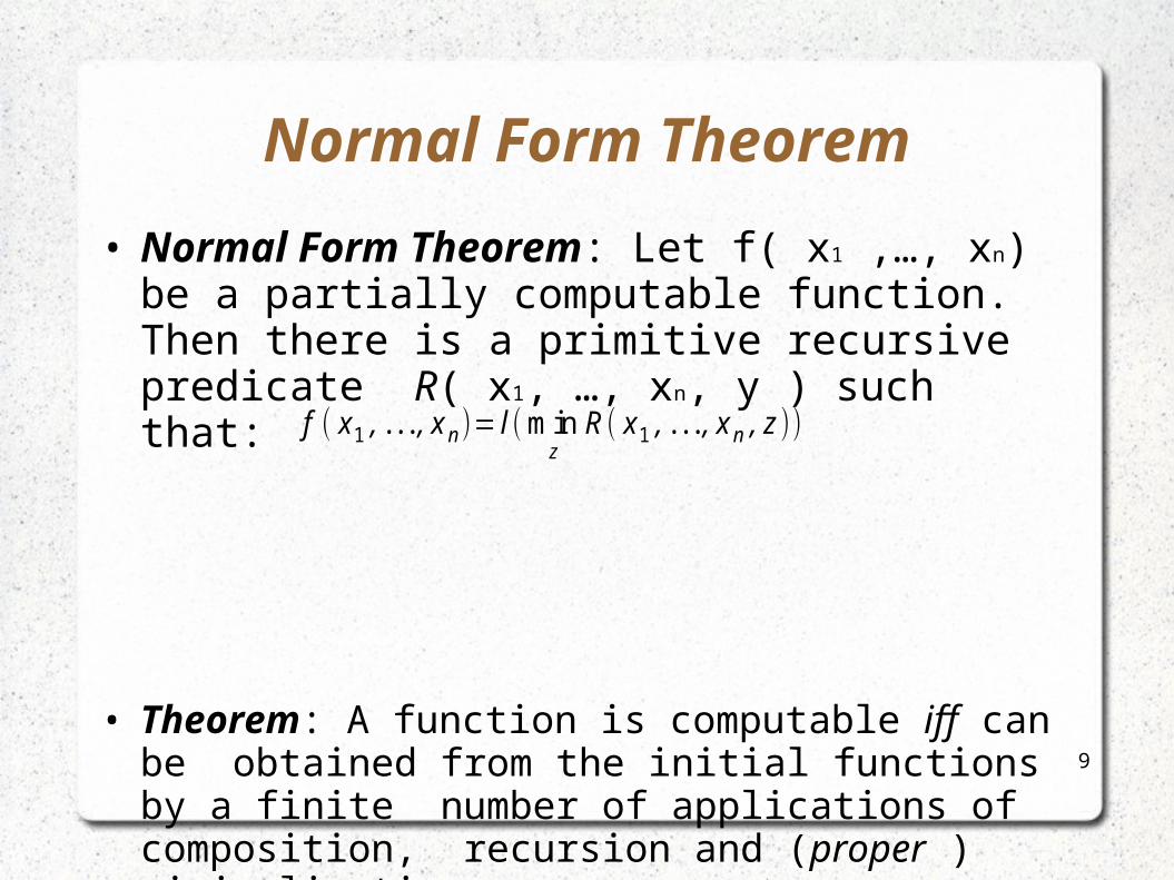
• Normal Form Theorem: Let f( x1 ,…, xn) be a partially computable function. Then there is a primitive recursive predicate R( x1, …, xn, y ) such that:

• Theorem: A function is computable iff can be obtained from the initial functions by a finite number of applications of composition, recursion and (proper ) minimalization

f ( x1 , . . . , x n )= l ( minz

R ( x1 , . . . , x n , z ))

9

Normal Form Theorem

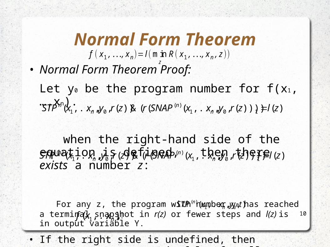
• Normal Form Theorem Proof:

Let y0 be the program number for f(x1,…,xn).

when the right-hand side of the equation is defined, then there exists a number z:

For any z, the program with number y0 has reached a terminal snapshot in r(z) or fewer steps and l(z) is in output variable Y.

• If the right side is undefined, then is false for all t i.e.

f ( x1 , . . . , x n )= l ( minz

R ( x1 , . . . , x n , z ))

10

)())))(,,,...,(((&))(,,,...,( 101)(

01 zlzryxxSNAPrzryxxSTP nn

nn

)())))(,,,...,(((&))(,,,...,( 101)(

01)( zlzryxxSNAPrzryxxSTP n

nn

n

),,,...,( 01)( tyxxSTP n

n

),...,( 1 nxxf

Recursively Enumerable Sets• Theorem: Let the sets B , C belong to some PRC class

C. Then so do the sets

(prove using predicate union and intersection)

• Theorem: Let C be a PRC class, and let B be a subset of . Then B belongs to C iff:

• Definition: The set is called recursively enumerable if there is a partially computable function g(x) such that:

1m,N m

B)x,,(x|N]x,,[x=B mm' ...... 11

belongs to C

NB

}{ g(x)|Nx=B

BCBCB ,,

11

Recursively Enumerable Sets

• If B is a recursive set, then B is recursively enumerable.

• The set B is recursive iff B and are both recursively enumerable.

• If B and C are recursively enumerable sets so are

• Enumeration Theorem: A set B is recursively enumerable iff there is an n for which B = Wn

B

CBCB ,

}),(|{ nxNxWn

12

Recursively Enumerable Sets

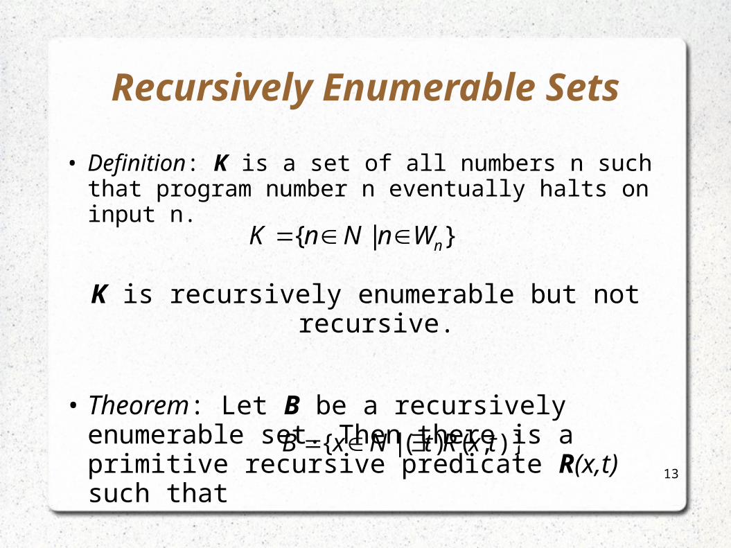
• Definition: K is a set of all numbers n such that program number n eventually halts on input n.

K is recursively enumerable but not recursive.

• Theorem: Let B be a recursively enumerable set. Then there is a primitive recursive predicate R(x,t) such that

}|{ nWnNnK

)},()(|{ txRtNxB 13

Recursively Enumerable Sets

• Theorem: Let S be a nonempty recursively enumerable set. Then there is a primitive recursive function f(u) such that

S = { f(n) | n ϵ N} = { f(0) , f(1) , … }

, where S is the range of f.

• Theorem: Let f(x) be a partially computable function and let

S = { f(x) | f(x) ↓} , where S is the range. Then S is recursively enumerable.

14

Recursively Enumerable Sets

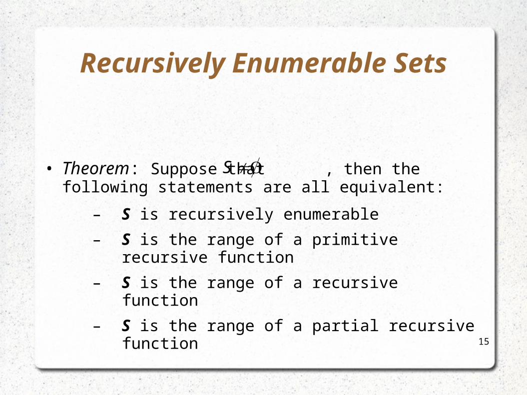
• Theorem: Suppose that , then the following statements are all equivalent:

– S is recursively enumerable

– S is the range of a primitive recursive function

– S is the range of a recursive function

– S is the range of a partial recursive function

S

15

The Parameter Theorem

• s-m-n Theorem:

For each n , m > 0 there is a primitive recursive function such that:),,...,,( 21 yuuuS n

nm

)),,...,(,,...,(),,...,,,...,( 11)(

11)( yuuSxxyuuxx n

nmm

mnm

nm

16

The Parameter Theorem• s-m-n proof: using induction on n.

Base case: For program P take n = 1, then the following must be shown to be true:

• should be the number of the program with m inputs

, which must be the same as program number y having m + 1 inputs .

• #(P) = y

• So will be the number of the program, that will provide the variable before proceeding with P.

17

)),(,,...,(),,,...,( 11

)(1

)1( yuSxxyuxx mmm

mm

),(1 yuSm

mxx ,...,1

uxx m ,,...,1

),(1 yuSm

1m

u

XX

XX

mm

mm

1

1

11

11

The Parameter Theorem• s-m-n proof: continued…

• The instruction will have a number associated with it as follows: <0,<1,2m+1>> = 16m + 10

• Thus may be defined as a primitive recursive function:

• Induction step: let n = k, then:

18

111 mm XX

),(1 yuSm

1),()1(

1

)1(1016

1

1

yLt

j

yju

mu

iim

jppyuS

)),(,,...,,,...,(),,,...,,,...,( 1

111

)(111

)1(kkmkm

kmkkm

km uSuuxxyuuuxx

))),(,,...,(,,...,( 11

11)( yuSuuSxx kkmk

kmm

m

),,,...,(,,...,( 111

1)( yuuuSxx kk

kmm

m

Diagonalization and Reducibility

• Definition: Let TOT be the set of all numbers p such that p is the number of a program that computes a total function f(x) of one variable. That is,

, where

• Theorem: TOT is not recursively enumerable.

}),()(|{ zxxNzTOT

,szWxzx ),(

19

Diagonalization and Reducibility

• Theorem: TOT is not recursively enumerable.

• Proof: Assume that TOT is recursively enumerable. Then given that , then there is a computable function g(x):

and let:

• Since g(x) is the number of a program that computes a total function, thus h is a computable function. Let P be the program that computes h and p=#(P). Then

Contradiction!

}),()(|{ zxxNzTOT

20

TOT

),...}2(),1(),0({ gggTOT

1))(,()( xgxxh

.)(, isomeforigpthatsoTOTp

1)(1),(1))(,()( ihpiigiih

Diagonalization and Reducibility

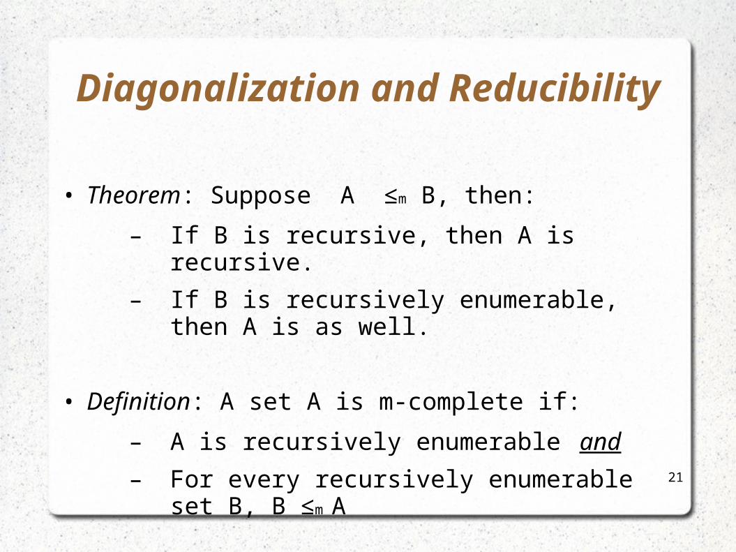
• Theorem: Suppose A ≤m B, then:

– If B is recursive, then A is recursive.

– If B is recursively enumerable, then A is as well.

• Definition: A set A is m-complete if:

– A is recursively enumerable and

– For every recursively enumerable set B, B ≤m A

21

Diagonalization and Reducibility

• If A ≤m B and B ≤m C, then A ≤m C (transitivity)

• If A is m-complete, B is recursively enumerable and A ≤m B then B is m-complete.

• Definition: A B means that A ≤m B and B ≤m A

• Theorem:

• K and K0 are m-complete

• K K0

• Theorem: EMPTY is not recursively enumerable, where

m

m

}|{ xWNxEMPTY22

Rice's Theorem

Examples:

• Г is the set of computable functions

• Г is the set of primitive recursive functions

• Г is the set of partially computable functions that are defined for all but a finite number of values of x

• Rice’s Theorem: Let Г be a collection of partially computable functions of one variable, such that there are functions f(x), g(x) with f(x) in Г, g(x) not in Г. Then RГ is not recursive.

• Corollary: There are no algorithms for testing a given program P of the language L to determine whether belongs to any of the classes described in the above examples.

• What does it mean? If Г is a non-trivial property of functions, then Г is undecidable.

}|{ tNtR

)()1( x

23

Rice's Theorem

Proof (using recursion theorem):

Let f(x) and g(x) be partially computable functions such that:

• f(x) Г

• g(x) Г

Suppose is computable. Let

and

Then, since

- is partially computable.

}|{ tNtR

R Iis not recursive

otherwise

RtiftP Г

Г 0

1)(

R

otherwisexf

Rtifxgxth Г

)(

)(),(

))(()()()(),( tPxftPxgxth ГГ

),( xth

Rice's Theorem

Proof (cont’d):

Since is partially computable, by recursion theorem there is a number

e s.t.:

As and :

Contradiction!

}|{ tNtR

),( xth

otherwisexf

ifxgxehx e

e )(

)(),()(

)(xf )(xg

Reimplies

inisximplies

xfximpliesRe

likewiseBut

Reimplies

innotisximplies

xgximpliesRe

e

e

e

e

)(

)()(

,

)(

)()(

26

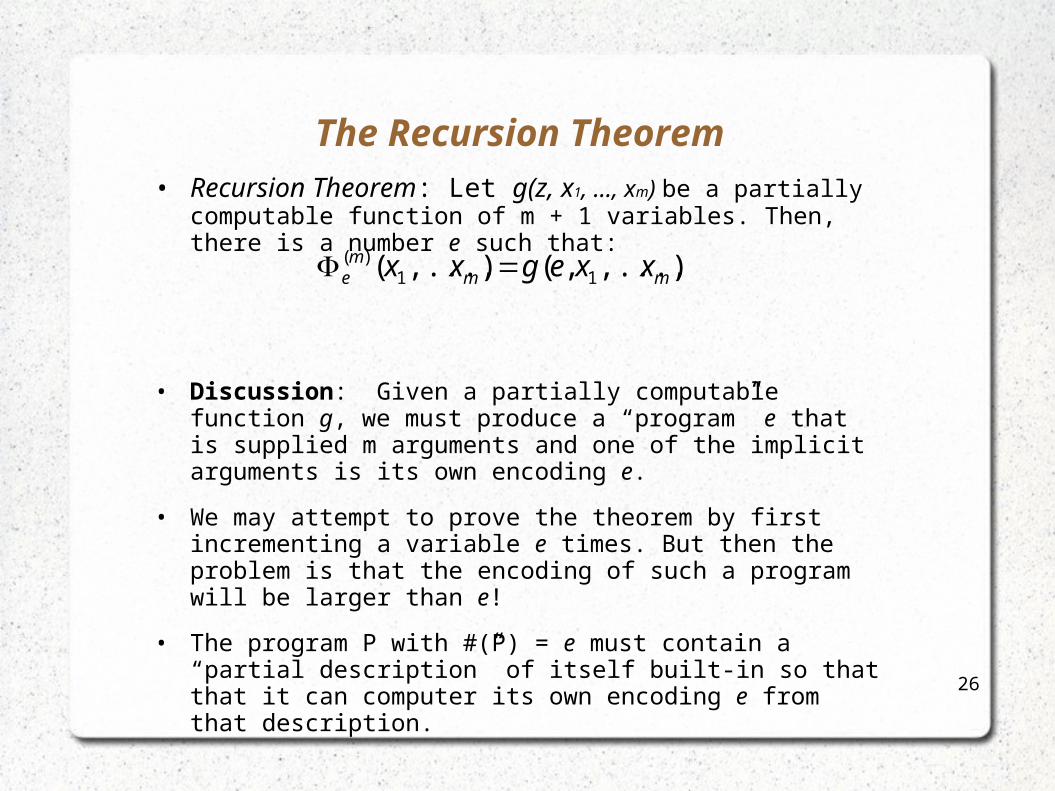
The Recursion Theorem• Recursion Theorem: Let g(z, x1, …, xm) be a partially computable

function of m + 1 variables. Then, there is a number e such that:

• Discussion: Given a partially computable function g, we must produce a “program” e that is supplied m arguments and one of the implicit arguments is its own encoding e.

• We may attempt to prove the theorem by first incrementing a variable e times. But then the problem is that the encoding of such a program will be larger than e!

• The program P with #(P) = e must contain a “partial description” of itself built-in so that that it can computer its own encoding e from that description.

),...,,(),...,( 11)(

mmm

e xxegxx

27

Let Q be the program: Z =

Y = g(Z, X1, X2, …, Xm)

Now, the program P will consist of #(Q) copies of the instruction Xm+1 = Xm+1 + 1, followed by the program Q.

After executing the first #(Q) increments as well as the instruction Z = …, Z holds the number of the program consisting of the #(Q) copies of the instruction followed by the program Q

(Remember that as defined in the proof of the parameter theorem computes the # of the program consisting of #(Q) copies of the increment instruction Xm+1 = Xm+1 + 1 followed by program Q).

But this is exactly the program P.

),( 111

mmm XXS

))(#),((#1 QQSm

The Recursion Theorem

Proof: Let g be a partially computable function such as:

is the function in the parameter theorem. Then for some z0 and using s-m-n theorem:

Set v = z0 and , then:

Contradiction!28

),...,),,(( 11

mm xxvvSg

)),(,,...,(),,,...,(),...,),,(( 01

101)1(

11 zvSxxzvxxxxvvSg mm

mm

mmm

),( 001 zzSe m

),...,(),,...,(),...,,( 1)(

1)(

1 mm

emm

m xxexxxxeg

1mS

The Recursion Theorem

• Corollary: There is a number e such that for all x:

• Proof: Let g be a computable function:

Using the recursion theorem:

• Fixed Point Theorem: Let f(z) be a computable function. Then there is a number e such that:

Take g(z, x) =

exe )(

)()()( xx eef

29

zxzuxzg ),(),( 21

exegxe ),()(

)()( xzf

Computable functions that are not primitive recursive

• The primitive recursive functions are precisely the functions from the initial functions (see Chapter 3)

• Theorem: The unary primitive recursive functions are precisely those obtained from the initial functions s(x) = x + 1, n(x) = 0, l(x) , r(x) by applying the following three operations on unary functions:

– To go from f(x) and g(x) to f(g(x))

– To go from f(x) and g(x) to < f(x) , g(x) >

– To go from f(x) and g(x) to the function defined by the recursion

• Theorem: The function f( x , x ) + 1 is a computable function that is not primitive recursive.

0)0( h

evenistif

thg

oddistift

f

th1

2

1

,12

)1(

30