chapter 3 automated preference elicitation for decision making
TRANSCRIPT

Chapter 3
Automated Preference Elicitation for DecisionMaking
Miroslav Karny
Abstract. In the contemporary complex world decisions are made by an imperfect
participant devoting limited deliberation resources to any decision-making task. A
normative decision-making (DM) theory should provide support systems allowing
such a participant to make rational decisions in spite of the limited resources. Ef-
ficiency of the support systems depends on the interfaces enabling a participant to
benefit from the support while exploiting the gradually accumulating knowledge
about DM environment and respecting incomplete, possibly changing, participant’s
DM preferences. The insufficiently elaborated preference elicitation makes even the
best DM supports of a limited use. This chapter proposes a methodology of auto-
matic eliciting of a quantitative DM preference description, discusses the options
made and sketches open research problems. The proposed elicitation serves to fully
probabilistic design, which includes a standard Bayesian decision making.
Keywords: Bayesian decision making, fully probabilistic design, DM preference
elicitation, support of imperfect participants.
3.1 Introduction
This chapter concerns of an imperfect participant1, which solves a real-life decision-
making problem under uncertainty, which is worth of its optimising effort. The topic
has arisen from the recognition that a real participant often cannot benefit from so-
phisticated normative DM theories due to an excessive deliberation effort needed
Miroslav Karny
Institute of Information Theory and Automation,
Academy of Sciences of the Czech Republic, Pod vodarenskou vezı 4, 182 08 Prague 8,
Czech Republic
e-mail: [email protected]
1 A participant is also known as user, decision maker, agent. A participant can be human, an
artificial object or a group of both. We refer the participant as “it”.
T.V. Guy et al. (Eds.): Decision Making and Imperfection, SCI 474, pp. 65–99.
DOI: 10.1007/978-3-642-36406-8_3 c© Springer-Verlag Berlin Heidelberg 2013

66 M. Karny
for their mastering and for feeding them by DM elements2 they need. This obser-
vation has stimulated a long-term research, which aims to equip a participant with
automatic tools (intelligent interfaces) mapping its knowledge, DM preferences and
constraints on DM elements while respecting its imperfection, i.e. ability to devote
only a limited deliberation effort to a particular DM task. The research as well as
this chapter concentrates on the Bayesian DM theory because of its exceptional,
axiomatically justified, role in DM under uncertainty, e.g. [49].
The adopted concept of the ultimate solution considers creating an automated
supporting system, which covers the complete design and use of a decision-
generating DM strategy. It has to preserve the theoretically reachable DM qual-
ity and free the participant’s cognitive resources to tasks specific to its application
domain. This concept induces:
Requirement 1: The supporting system uses a consistent and complete DM theory.
Requirement 2: To model the environment3 the supporting system fully exploits
both participant’s knowledge and information brought by the data observed during
the use of the DM strategy.
Requirement 3: The supporting system respects participant’s DM preferences and
refines their description by the information gained from the observed data.
This chapter represents a further step to the ultimate solution. It complements the re-
sults of the chapter [28] devoted to DM of imperfect participants. The tools needed
for a conceptual solution are based on a generalised Bayesian DM, called fully prob-
abilistic design (FPD) [23, 29], see also Section 3.2. The FPD minimises Kullback-
Leibler divergence [38] of the optimised, strategy-dependent probabilistic model of
the closed DM loop on its ideal counterpart. which describes the desired behaviour
of the closed decision loop. The design replaces the maximisation of an expected
utility over a set of admissible decision strategies [4] for the FPD densely extend-
ing all standard Bayesian DM formulations [31]. The richness, intuitive plausibility,
practical advantages and axiomatic basis of the FPD motivate its acceptance as a
unified theoretical DM basis, which meets Requirement 1.
Requirement 2 concerns the description of the environment with which the partic-
ipant interacts during DM. Traditionally, its construction splits into a structural and
semi-quantitative modelling of the environment and knowledge elicitation under-
stood as a quantitative description of unknown variables entering the environment
model. Both activities transform domain-specific knowledge into the model-related
part of DM elements.
The environment modelling is an extremely wide field that exploits first princi-
ples (white and grey box models, e.g. [6, 22]), application-field traditions, e.g. [9],
2 This is a common label for all formal, qualitatively and quantitatively specified, objects
needed for an exploitation of the selected normative DM theory.3 The environment, also called system, is an open part of the World considered by the par-
ticipant and with which it interacts within the solved DM task.
3 Automated Preference Elicitation for Decision Making 67
universal approximation (black box models, e.g. [17, 50]) and their combinations.
An automated mapping of these models on probabilistic DM elements of the FPD is
the expected service of the supporting DM system. The tools summarised in [28] are
conjectured to be sufficient to this purpose. Knowledge elicitation in the mentioned
narrow sense is well surveyed in [14, 45] and automated versions related to this
chapter are in [24, 25]. The ordinary Bayesian framework [4, 47] adds the required
ability to learn from the observed data.
Requirement 3 reflects the fact that a feasible and effective solution of preference
elicitation problem decides on the efficiency of any intelligent system supporting
DM. This extracting the information about the participant’s DM preferences has
been recognised as a vital problem and repeatedly addressed within artificial intel-
ligence, game theory, operation research. Many sophisticated approaches have been
proposed [10, 11, 13, 16], often in connection with applied sciences like economy,
social science, clinical decision making, transportation, see, for instance, [21, 41].
Various assumptions on the structure of DM preferences have been adopted in or-
der to ensure feasibility and practical applicability of the resulting decision support.
Complexity of the elicitation problem has yet prevented to get a satisfactory widely-
applicable solution. For instance, the conversion of DM preferences on individual
observable decision-quality-reflecting attributes into the overall DM preferences is
often done by assuming their additive independence [33]. The DM preferences on
attributes are dependent in majority of applications and the enforced independence
assumption significantly worsens the elicitation results4. This example indicates a
deeper drawback of the standard Bayesian DM, namely, the lack of unambiguous
rules how to combine low-dimensional description of DM preferences into a global
one.
The inability of the participant to completely specify its DM preferences is an-
other problem faced. In this common case, the DM preferences should be learned
from either domain-specific information (technological requirements and knowl-
edge, physical laws, etc.) or the observed data.
Eliciting the needed information itself is an inherently difficult task, which suc-
cess depends on experience and skills of an elicitation expert. The process of elicit-
ing of the domain-specific information is difficult, time-consuming and error-prone
activity5. Domain experts provide subjective opinions, typically expressed in differ-
ent forms. Their processing requires a significant cognitive and computational effort
of the elicitation expert. Even if the cost of this effort6 is negligible, the elicitation
4 The assumption can be weakened by a introducing a conditional preferential independence,
[8].5 It should be mentioned that practical solutions mostly use a laborious and unreliable pro-
cess of manual tuning a number of parameters of the pre-selected utility function. The high
number of parameters makes this solution unfeasible and enforces attempts to decrease the
number to recover feasibility.6 This effort is usually very high and many sophisticated approaches aim at optimising a
trade-off between elicitation cost and value of information it provides (often, a decision
quality is considered), see for instance [7].
68 M. Karny
result is always limited by the expert’s imperfection, i.e. his/her inability to devote
an unlimited deliberation effort to eliciting. Unlike the imperfection of experts pro-
viding the domain-specific information, the imperfection of elicitation experts can
be eliminated by preparing a feasible automated support of the preference elicita-
tion, that does not rely on any elicitation expert.
The dynamic decision making strengthes the dependence of the DM quality on
the preference elicitation. Typically, the participant acting within a dynamically
changing environment with evolving parameters gradually changes its DM pref-
erences. The change may depend on the expected future behaviour or other circum-
stances. The overall task is getting even harder when the participant dynamically
interacts with other imperfect participants within a common environment. When
DM preferences evolve, their observed-data-based learning becomes vital.
The formal disparity of modelling language (probabilities) and the DM prefer-
ence description (utilities) makes Bayesian learning of DM preferences difficult.
It needs a non-trivial “measurement” of participant’s satisfaction of the decision re-
sults, which often puts an extreme deliberation load on the participant. Moreover, the
degree of satisfaction must be related to conditions under which it has been reached.
This requires a non-standard and non-trivial modelling. Even, if these learning ob-
stacles are overcome, the space of possible behaviour is mostly larger than that the
observed data cover. Then, the initial DM preferences for the remaining part of the
behaviour should be properly assigned and exploration has to care about making the
DM preference description more precise. Altogether, a weak support of the prefer-
ence elicitation (neglecting of Requirement 3) is a significant gap to be filled. Within
the adopted FPD, an ideal probability density (pd7) is to be elicited8. The ideal pd
describes the closed-loop behaviour, when the participant’s DM strategy is an opti-
mal one and the FPD searches for the optimal randomised strategy minimising the
divergence from the current closed-loop description to the ideal one.
Strengthening the support with respect to Requirement 3 forms the core of this
chapter. The focus on the preference elicitation for the FPD brings immediate
methodological advantages. For instance, the common probabilistic language for
knowledge and DM preference descriptions simplifies an automated elicitation as
the ideal pd provides a standardised form of quantitatively expressed DM pref-
erences. Moreover, the raw elicitation results reflect inevitably incomplete, com-
petitive or complementing opinions with respect to the same collection of DM
preference-expressing multivariate attributes. Due to their automated mapping on
probabilities, their logically consistent merging is possible with the tools described
in [28]. Besides, domain experts having domain-specific information are often
7 Radon-Nikodym derivative [48] of the strategy-dependent measure describing closed DM
loop with respect to a dominating, strategy-independent measure. The use of this notion
helps us to keep a unified notation that covers cases with mixed – discrete and continuous
valued – variables.8 Let us stress that no standard Bayesian DM is omitted due to the discussed fact that the
FPD densely covers all standard Bayesian DM tasks.

3 Automated Preference Elicitation for Decision Making 69
unable to provide their opinion on a part of behaviour due to either limited knowl-
edge of the phenomena behind or the indifference towards the possible instances
of behaviour. Then, the DM preference description has to be extended to the part
of behaviour not “covered” by the domain-specific information. This extension is
necessary as the search for the optimal strategy heavily depends on the full DM
preference description. It is again conceptually enabled by the tools from [28]. The
usual Bayesian learning is applicable whenever the DM preferences are related to
the observed data [27].
In summary, the chapter concerns a construction of a probabilistic description
of the participant’s DM preferences based on the available information. Decision
making under uncertainty is considered from the perspective of an imperfect partic-
ipant. It solves a DM task with respect to its environment and indirectly provides
a finite description of the DM preferences in a non-unique way9 and leaves uncer-
tainty about the DM preferences on a part of closed-loop behaviour. To design an
optimal strategy, the participant employs the fully probabilistic design of DM strate-
gies [23,29] whose DM elements are probability densities used for the environment
modelling, DM preference description and description of the observed data.
The explanations prefer discussion of the solution aspects over seemingly defi-
nite results. After a brief summary of common tools Section 3.2, they start with a
problem formalisation that includes the basic adopted assumptions, Section 3.3. The
conceptual solution summarised in Section 3.4 serves as a guide in the subsequent
extensive discussion of its steps in Section 3.5. Section 3.6 provides illustrative sim-
ulations and Section 3.7 contains concluding remarks.
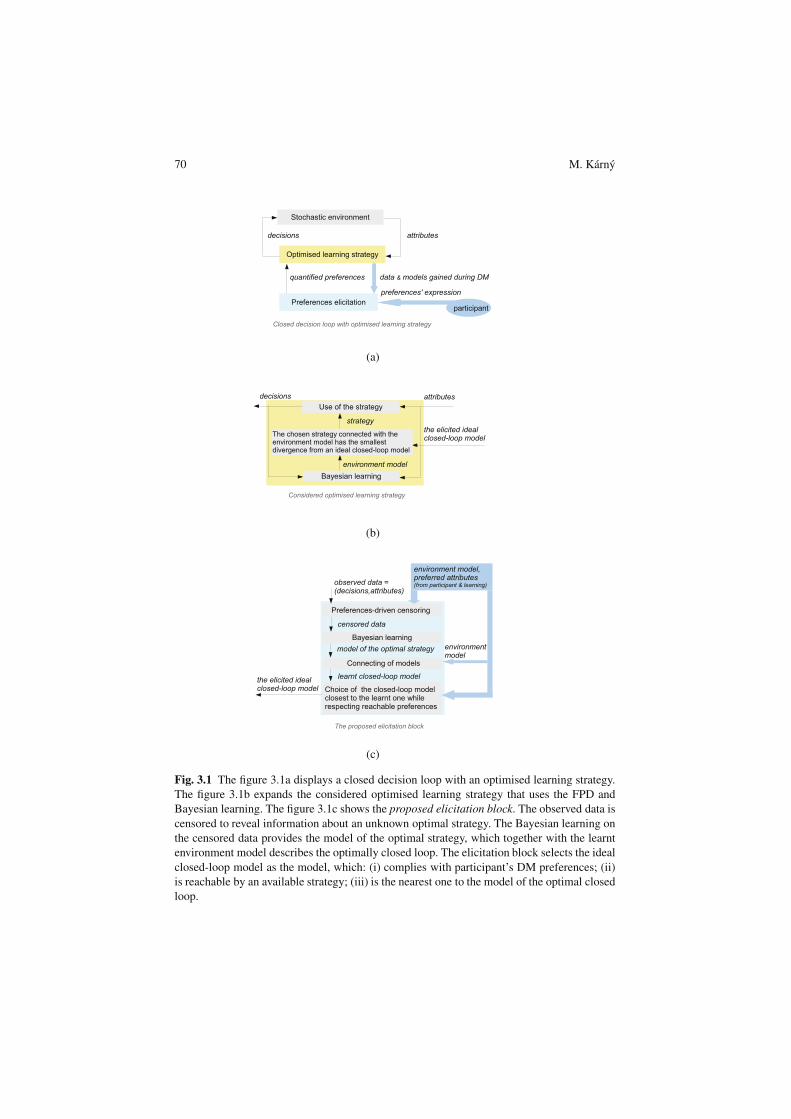
Concept of the proposed preference elicitation is reflected in Figure10 3.1.
The usual decision loop formed by a stochastic environment and a decision strat-
egy complemented by a preference elicitation block is expanded to the proposed
solution. The considered strategy consists of the standard Bayesian learning of the
environment model and of a standard fully probabilistic design (FPD). Its explicit
structuring reveals the need of the ideal closed-loop model of the desired closed-
loop behaviour. The designed strategy makes the closed decision loop closest to this
ideal model, which is generated by the elicitation block as follows. The observed
data is censored11 to data, which contains an information about the optimal strategy
and serves for its Bayesian learning. The already learnt environment model is com-
bined with the gained model of the optimal strategy into the model of the DM loop
closed by it. Within the set of closed-loop models, which comply with the partici-
pant’s DM preferences and are believed to be reachable, the ideal closed-loop model
is selected as the nearest one to the learnt optimal closed-loop model.
9 Even, when we identify instances of behaviour that cannot be preferentially distinguished.10 A block performing the inevitable knowledge elicitation is suppressed to let the reader
focus on the proposed preference elicitation.11 Such data processing is also called filtering. This term is avoided as it has also another
meaning.
70 M. Karny
(a)
(b)
(c)
Fig. 3.1 The figure 3.1a displays a closed decision loop with an optimised learning strategy.
The figure 3.1b expands the considered optimised learning strategy that uses the FPD and
Bayesian learning. The figure 3.1c shows the proposed elicitation block. The observed data is
censored to reveal information about an unknown optimal strategy. The Bayesian learning on
the censored data provides the model of the optimal strategy, which together with the learnt
environment model describes the optimally closed loop. The elicitation block selects the ideal
closed-loop model as the model, which: (i) complies with participant’s DM preferences; (ii)
is reachable by an available strategy; (iii) is the nearest one to the model of the optimal closed
loop.

3 Automated Preference Elicitation for Decision Making 71
Notation
General conventionsxxx is a set of x-values having cardinality |xxx|
d ∈ ddd, ddd , ∅ are decisions taken from a finite-dimensional set ddd
ai ∈ aaai, i ∈ iii = 1, . . . , |iii| are attribute entries in finite-dimensional sets aaai
a ∈ aaa is a collection of all attributes in the set aaa = Xi∈iiiaaai,
X denotes the Cartesian product
ααα $ aaa, ααα , ∅ is the set of the most desirable attribute values specified
entry-wise ααα = Xi∈iiiαααi
t ∈ ttt = 1, . . . , |ttt| is discrete time
(xt)t∈ttt is a sequence of xt indexed by discrete time t ∈ ttt.
Probability densities
g(·),h(·) are probability densities (pds): Radon-Nikodym derivatives
with respect to a dominating measure denoted d·
Mt(a|d), M(a|d,Θ) are the environment model and its parametric version with
an unknown parameter Θ ∈ΘΘΘ
Ft(Θ), t ∈ ttt∪0 is the pd quantifying knowledge available at time t about
the unknown parameter Θ of the environment model
St(d) describes the randomised decision strategy to be selected
st(d), s(d|θ) are the model of the optimal strategy and its parametric version
with an unknown parameter θ ∈ θθθ
ft(θ), t ∈ ttt∪0 is the pd quantifying knowledge available at time t about
the unknown parameter θ ∈ θθθ of the optimal strategy
It(a,d) is the ideal pd quantifying the elicited participant’s DM
preferences
Pt(a,d) is the pd modelling the decision loop with the optimal strategy
Mt(ai|d), It(ai), i ∈ iii are marginal pds of ai derived from pds Mt(a|d) and It(a,d)
Convention on time indexing
Ft−1(Θ), ft−1(θ) quantify knowledge accumulated before time t
Mt(a|d), st(d), St(d) serve to the tth DM task and exploit
It(a,d), Pt(a,d) the knowledge accumulated before time t.
Frequent symbols
d ∈ ddd is a decision leading to a high probability of the set ααα
D(h||g) is the Kullback-Leibler divergence (KLD, [38]) of a pd
h from a pd g
E[·] denotes expectation
V is a sufficient statistic of the exponential family (EF),
which becomes the occurrence table in Markov-chain case
φ ∈ [0,1] is a forgetting factor
∝ denotes an equality up to normalisation.

72 M. Karny
3.2 Preliminaries
Introduction repeatedly refers to the tools summarised in [28]. Here, we briefly re-
call its sub-selection used within this chapter.
1. The Kullback-Leibler divergence (KLD, [38]) D(g||h) of a pd g from a pd h, both
defined on a set xxx and determined by a dominating strategy-independent measure
dx, is defined by the formula
D(g||h) =
∫
xxx
g(x) ln
(
g(x)
h(x)
)
dx. (3.1)
The KLD is a convex functional in the pd g, which reaches its smallest zero value
iff g = h dx-almost everywhere.
D(g||h),D(h||g) and a correct pd should be used as its first argument when mea-
suring (di)similarity of pds by the KLD. A pd is called correct12 if it fully exploits
the knowledge about the random variable it models. Its existence is assumed.
2. Under the commonly met conditions [5], the optimal Bayesian approximation
ho ∈ hhh of a correct pd g by a pd h ∈ hhh should be defined
ho ∈ Argminh∈hhhD(g||h). (3.2)
3. The minimum KLD principle [28, 51] recommends to select a pd he ∈ hhh
he ∈ Argminh∈hhhD(h||g) (3.3)
as an extension of the available information about the correct pd h. The assumed
available information consists of a given set hhh and of a rough (typically flat)
estimate g of the pd h.
The minimum KLD principle provides such an extension of the available infor-
mation that the pd he deviates from its estimate g only to the degree enforced by
the constraint h ∈ hhh. It reduces to the celebrated maximum entropy principle [20]
for the uniform pd g.
The paper [51] axiomatically justifies the minimum KLD principle for sets hhh
delimited by values of h moments. The generalisation in [28] admits a richer
collection of the sets hhh. For instance, the set hhh can be of the form
hhh =
h : D(
h||h)
≤ k <∞
, (3.4)
determined by a given pd h and by a positive constant k.
For the set (3.4), the pd he (3.3) can be found by using the Kuhn-Tucker optimal-
ity conditions [35]. The solution reads
he ∝ hφg1−φ, φ ∈ [0,1], (3.5)
12 This is an operational notion unlike often used adjectives “true” or “underlying”.

3 Automated Preference Elicitation for Decision Making 73
where ∝ denotes an equality up to a normalisation factor and φ is to be chosen
to respect the constraint (3.4). The solution formally coincides with the so-called
stabilised forgetting [37] and φ is referred as forgetting factor.
3.3 Problem Formalisation
The considered participant repeatedly solves a sequence of static13 DM tasks in-
dexed by (discrete) time t ∈ ttt = 1,2, . . . , |ttt|. DM concerns a stochastic, incompletely-
known, time-invariant static environment. The decision d influencing the environ-
ment is selected from a finite-dimensional set ddd. The participant judges DM quality
according to a multivariate attribute a ∈ aaa, which is a participant-specified image of
the observed environment response to the applied decision. The attribute has |iii| <∞,
possibly vectorial, entries ai. Thus, a = (ai)|iii|
i=1, ai ∈ aaai, i ∈ iii = 1, . . . , |iii|, and aaa is the
Cartesian product aaa = Xi∈iiiaaai.
The solution of a sequence of static DM tasks consists of the choice and use of
an admissible randomised strategy, which is formed by a sequence (St)t∈ttt of the
randomised causal mappings
St ∈SSSt ⊂ knowledge available at time (t−1)→ dt ∈ ddd, t ∈ ttt. (3.6)
We accept the following basic non-restrictive assumptions.
Agreement 1 (Knowledge Available). The knowledge available at time (t − 1)
(3.6), t ∈ ttt, includes
• the data observed up to time (t − 1) inclusive, i.e. decisions made (d1, . . . ,dt−1)
and the corresponding realisations of attributes (a1, . . . ,at−1);
• a time-invariant parametric environment model M(a|d,Θ) > 0, which is a condi-
tional pd known up to a finite-dimensional parameter Θ ∈ΘΘΘ;
• a prior pd F0(Θ) > 0 on the unknown parameter Θ ∈ΘΘΘ.
The standard Bayesian learning and prediction [47] require availability of the
knowledge described in Agreement 1 in order to provide the predictive pds
(Mt(a|d))t∈ttt. They model the environment in the way needed for the design of the
admissible strategy (St)t∈ttt.
Agreement 2 (Optimality in the FPD Sense). The following optimal strategy(
Sot
)
t∈ttt in the FPD sense [31] is chosen
(
Sot
)
t∈ttt ∈ Arg min(St∈SSSt)t∈ttt
1
|ttt|
∑
t∈ttt
E[D(MtSt||It)], (3.7)
13 The restriction to the static case allows us to avoid technical details making understanding
of the conceptual solution difficult. All results are extendable to the dynamic DM with
a mixed (discrete and continuous) observed data and considered but unobserved internal
variables.

74 M. Karny
where the participant’s DM preferences in tth DM task are quantified by an ideal pd
It(a,d) assigning a high probability to the desirable pairs (a,d) ∈ (aaa,ddd) and a low
probability to undesirable ones. The expectation E[•] is taken over conditions of the
individual summands in (3.7)14.
The strategy(
Sot
)
t∈ttt minimises an average Kullback-Leibler divergence D(MtSt||It)
of the strategy-dependent closed-loop model Mt(a|d)St(d) from the participant’s
DM preferences-expressing ideal pd It(a,d).
Assumption 1 (Preference Specification). The participant provides the time-inva-
riant sets αααi, i ∈ iii, of the most desirable values of individual attribute entries ai
αααi ⊂ aaai, αααi , ∅, i ∈ iii. (3.8)
These sets define the set of the most desirable attributes’ values ααα
ααα = Xi∈iiiαααi $ aaa, ααα , ∅. (3.9)
The participant can also assign importance weights w ∈ www = w = (w1, . . . ,w|iii|),
wi ≥ 0,∑
i∈iii wi = 115 to particular attribute entries but the availability of w is rarely
realistic.
Generally, the participant may specify a number of not necessarily embedded sets
αααµ, µ ∈ µµµ = 1, . . . , |µµµ|, |µµµ| > 1, of the desirable attribute values with the desirability
decreasing with µ. The participant may also specify similar information about the
possible decisions. The chosen version of the partially specified DM preferences
suffices for presenting an essence of the proposed approach.
Preferences are elicited under the following non-standard assumption.
Assumption 2 (Modelling of the Unknown Optimal Strategy). A parametric
model s(d|θ) of an unknown optimal randomised strategy and a prior pd f0(θ) of
an unknown finite-dimensional θ ∈ θθθ parameterising this model are available.
The feasibility of Assumption 2 follows from the time-invariance of the parametric
model of the environment and from the assumed invariance of the (partially speci-
fied) participant’s DM preferences16. Neither the environment model nor the com-
plete DM preferences are known and the parameter. The only source of knowledge
is observed closed-loop data. Therefore the model of the optimal strategy can be
learnt from it during application of non-optimal strategy. Having this non-standard
learning problem solved, the standard Bayesian prediction [47] provides the model
of the optimal strategy as the predictive pd st(d). The chain rule [47] for pds and the
already learnt environment model Mt(a|d) imply the availability of the closed-loop
model with the estimated optimal strategy st(d)
14 The considered KLD measures divergence between the conditional pds. The environment
model Mt(a|d), the optimised mapping St(a) as well as the ideal pd It(a,d) depend on the
random knowledge available at time (t−1), see Agreement 1.15 The set is referred as probabilistic simplex.16 The proposed preference elicitation with time-invariant sets αααi can be extended to time-
varying cases.
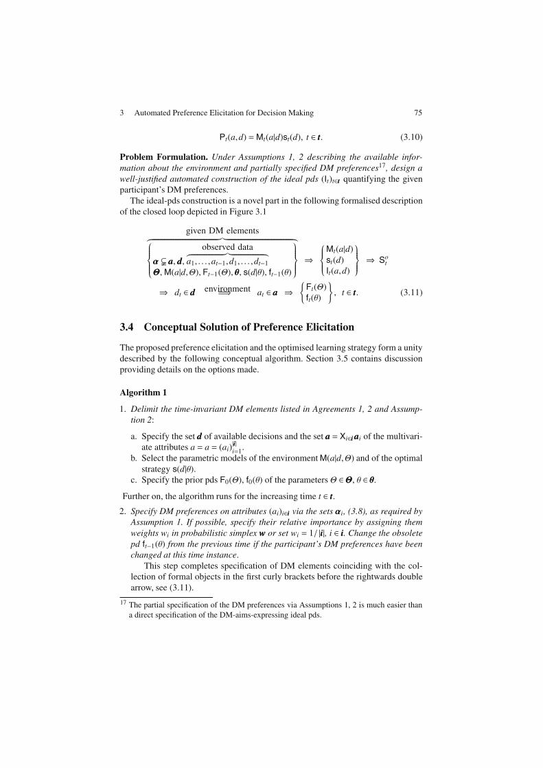
3 Automated Preference Elicitation for Decision Making 75
Pt(a,d) =Mt(a|d)st(d), t ∈ ttt. (3.10)
Problem Formulation. Under Assumptions 1, 2 describing the available infor-
mation about the environment and partially specified DM preferences17, design a
well-justified automated construction of the ideal pds (It)t∈ttt quantifying the given
participant’s DM preferences.
The ideal-pds construction is a novel part in the following formalised description
of the closed loop depicted in Figure 3.1
given DM elements︷ ︸︸ ︷
ααα $ aaa, ddd,
observed data︷ ︸︸ ︷
a1, . . . ,at−1,d1, . . . ,dt−1
ΘΘΘ,M(a|d,Θ), Ft−1(Θ), θθθ, s(d|θ), ft−1(θ)
⇒
Mt(a|d)
st(d)
It(a,d)
⇒ Sot
⇒ dt ∈ ddd =⇒environment at ∈ aaa ⇒
Ft(Θ)
ft(θ)
, t ∈ ttt. (3.11)
3.4 Conceptual Solution of Preference Elicitation
The proposed preference elicitation and the optimised learning strategy form a unity
described by the following conceptual algorithm. Section 3.5 contains discussion
providing details on the options made.
Algorithm 1
1. Delimit the time-invariant DM elements listed in Agreements 1, 2 and Assump-
tion 2:
a. Specify the set ddd of available decisions and the set aaa = Xi∈iiiaaai of the multivari-
ate attributes a = a = (ai)|iii|
i=1.
b. Select the parametric models of the environment M(a|d,Θ) and of the optimal
strategy s(d|θ).
c. Specify the prior pds F0(Θ), f0(θ) of the parameters Θ ∈ΘΘΘ, θ ∈ θθθ.
Further on, the algorithm runs for the increasing time t ∈ ttt.
2. Specify DM preferences on attributes (ai)i∈iii via the sets αααi, (3.8), as required by
Assumption 1. If possible, specify their relative importance by assigning them
weights wi in probabilistic simplex www or set wi = 1/ |iii|, i ∈ iii. Change the obsolete
pd ft−1(θ) from the previous time if the participant’s DM preferences have been
changed at this time instance.
This step completes specification of DM elements coinciding with the col-
lection of formal objects in the first curly brackets before the rightwards double
arrow, see (3.11).
17 The partial specification of the DM preferences via Assumptions 1, 2 is much easier than
a direct specification of the DM-aims-expressing ideal pds.

76 M. Karny
3. Evaluate predictive pds, [47], Mt(a|d), st(d) serving as the environment model
and the optimal-strategy model.
The models Mt(a|d), st(d), serve for a design of St (3.6) generating the deci-
sion dt. Thus, they can exploit data measured up to and including time t− 1, cf.
Agreement 1.
4. Select a decision d = d(w) (it depends on the weights w assigned)
d = d(w) ∈ Argmaxd∈ddd
∑
i∈iii
wi
∫
αααi
Mt(ai|d)dai (3.12)
and define the set IIIt of the reachable ideal pds expressing the participant’s DM
preferences
IIIt =
It(a,d) : It(ai) =Mt
(
ai|d)
, ∀ai ∈ aaai, i ∈ iii
. (3.13)
The decision d ∈ ddd provides the Pareto-optimised probabilities18
∫
ααα1
Mt(a1|d)da1, . . . ,
∫
ααα|iii|
Mt(a|iii||d)da|iii|
of the desirable attribute-entries sets (3.8). The weight w with constant entries
wi = 1/ |iii| can be replaced by the weight wo maximising the probability of the set
ααα = Xi∈iiiαααi of the most desirable attribute values
wo ∈ Argmaxw∈www
∫
ααα
Mt(a|d(w))da,
see (3.12).
5. Extend the partial specification It ∈ IIIt, (3.13) to the pd Iet (a,d) via the following
application of the minimum KLD principle
Iet ∈ ArgminIt∈IIItD(It||Pt) with Pt(a,d) =Mt(a|d)st(d). (3.14)
The set IIIt created in Step 4 reflects the participant’s DM preferences. The ex-
tension to the ideal pd Iet (a,d) supposes that st is a good guess of the optimal
strategy.
This step finishes the specification of the mapping marked by the first right-
wards double arrow in (3.11).
6. Perform the FPD (3.7) with the environment model Mt(a|d) and the ideal pd
Iet (a,d). Then generate dt according to the mapping Sot optimal in the FPD sense
(3.7), apply it, and observe at.
Enriching the knowledge available makes the solved DM task dynamic one
even for the time-invariant parametric environment model. The dynamics is en-
hanced by the dependence of the used ideal pd on data and time. The unfeasible
18 A vector function, dependent on a decision, becomes Pareto-optimised if an improvement
of any of its entries leads to a deterioration of another one, [46].

3 Automated Preference Elicitation for Decision Making 77
optimal design arising for this complex dynamic DM task has to be solved ap-
proximately and the approximation should be revised at each time moment.
This step finishes the specification of the mappings symbolised by the second
and marked by the third rightwards double arrow in (3.11).
7. Update the pd Ft−1(Θ) →(at ,dt) Ft(Θ) in the Bayesian way, i.e. enrich the knowl-
edge about the parameter Θ of the environment model M(a|d,Θ) by at,dt.
This step is inevitable even when making decisions without the preference elici-
tation. The updating may include forgetting [37] if the parameterΘ varies.
8. Update the information about the parameter of the model of the optimal strategy,
i.e. update ft−1(θ)→(at ,dt) ft(θ) according to the following weighted version of the
Bayes rule19
ft(θ) ∝ sφt (d|θ)ft−1(θ), φt =
∫
ααα
Mt+1(a|d = dt)da. (3.15)
This data censoring is inevitable for learning the optimal strategy.
The step finishes the specification of the mapping expressed by the last right-
wards double arrow in (3.11).
9. Increase time t and go to Step 2 or to Step 3, if the DM preferences have not been
changed.
3.5 Individual Steps of the Conceptual Solution
This section provides details and discussion of the solution steps. The following
sections correspond to the individual steps of the conceptual solution summarised
in Section 3.4. The third digit of a section coincides with the corresponding number
of the discussed step. Steps 2, 4, 5, 6 and 8 are the key ones, the remaining are
presented for completeness.
The general solution is specialised to the important parametric models from the
exponential family [2] used in the majority of practically feasible solutions.
3.5.1 Specification of Decision Making Elements
This step transforms a real-life DM task formulated in domain-oriented terms into
the formal one.
ad 1a Specification of the sets of available decisionsddd and observable attributesaaa
Often, these sets are uniquely determined by the domain-specific conditions of
the solved DM task. Possible ambiguities can be resolved by Bayesian testing
of hypothesis, e.g. [32], about informativeness of the prospective attributes and
about influence of the available decisions.
19 The environment model Mt+1(a|d = dt) used in (3.15) exploits data measured up to and
including time t and will also serve for the choice of dt+1.

78 M. Karny
ad 1b Choice of the parametric models M(a|d,Θ), Θ ∈ΘΘΘ, s(d|θ), θ ∈ θθθ
A full modelling art, leading to grey- or black-box models, can be applied here.
The modelling mostly provides deterministic but approximate models, which
should be extended to the needed probabilistic models via the minimum KLD
principle, Section 3.2.
Illustrative simulations, Section 3.6, use zero-order Markov chains that re-
late discrete-valued attributes and decisions. Markov chains belong to a dynamic
exponential family (EF)20, [2, 26],
M(at|a1, . . . ,at−1,d1, . . . ,dt,Θ) =M(at|dt,Θ) = exp〈B(at,dt),C(Θ)〉 , (3.16)
determined by a scalar product 〈B,C〉 of compatible values of multivariate func-
tions B(a,d)21 and C(Θ).
The following formula provides the considered most general parametrisation
of Markov-chain models and its correspondence with the EF
M(at|dt,Θ) = Θ(at|dt) = exp
∑
a∈aaa,d∈ddd
δ(a,at)δ(d,dt) ln(Θ(a|d))
= exp〈B(at,dt),C(Θ)〉 , Θ ∈ΘΘΘ, (3.17)
s(dt|θ) = exp
∑
d∈ddd
δ(d,dt) ln(θ(d))
= exp〈b(dt),c(θ)〉 , θ ∈ θθθ,
where b, c have the same meaning as B, C in (3.16).ΘΘΘ, θθθ are in appropriate prob-
abilistic simplex sets and Kronecker delta δ(x, x) equals to one for x = x and it is
zero otherwise.
ad 1c Specification of prior pds F0(Θ), f0(θ), Θ ∈ΘΘΘ, θ ∈ θθθ
The specification of the prior pds is known as knowledge elicitation. A rela-
tively complete elaboration of the automated knowledge elicitation (focused on
the dynamic EF) is in [24]. Comparing to a general case, the knowledge elicita-
tion problem within the EF is much simpler as the EF admits a finite-dimensional
sufficient statistic [34] and possesses a conjugate prior pd [4]. It has the following
self-reproducing functional form
F0(Θ) ∝ exp〈V0,C(Θ)〉χΘΘΘ(Θ), f0(Θ) ∝ exp〈v0,c(θ)〉χθθθ(θ) (3.18)
where an indicator function χxxx(x) equals one for x ∈ xxx and is zero otherwise.
In the EF, the knowledge elicitation reduces to a selection of finite-dimensional
tables V0,v0 parameterising these prior pds.
20 Models from the EF dominate in practice.21 The dependence only on dt formalises the assumed static case. In a fully dynamic case, the
function B acts on values of a finite-dimensional function of the observed data and of the
current decision. Its dimension is fixed even for growing number of collected data and its
values can be updated recursively.

3 Automated Preference Elicitation for Decision Making 79
For Markov chains, the conjugate priors are Dirichlet pds, cf. (3.17). Their
functional forms (chosen for t = 0) are preserved for all t ∈ ttt
Ft(Θ) =∏
d∈ddd
∏
a∈aaaΘ(a|d)Vt(a|d)−1
β(Vt(·|d))χΘΘΘ(Θ) =
∏
d∈ddd
DiΘ(·|d)(Vt(·|d))
Vt(·|d) = (Vt(a1|d), . . . ,Vt(a|iii||d)), Θ(·|d) = (Θ(a1|d), . . . ,Θ(a|iii||d)), ai ∈ aaai,
ft(θ) = Diθ(vt), V0(a|d) > 0, v0(d) > 0 on aaa,ddd. (3.19)
The used multivariate beta function
β(x) =
∏
l∈lll Γ(xl)
Γ(∑
l∈lll xl
)
is defined for a positive |lll|-vector x. Γ(·) is Euler gamma function [1]. V0 can be
interpreted as an occurrence table: V0(a|d) means the (thought) number of occur-
rences of the value a following the decision d. v0 has a similar interpretation.
3.5.2 Specification of Preferences and Their Changes
The domain-specific description of the participant’s DM preferences via the set
(αααi)i∈iii of the most desirable attribute values (3.8) is a relatively straightforward task.
The considered entry-wise specification respects limits of the human being, who
can rarely go beyond pair-wise comparison. The DM preferences specified by (3.8)
mean
αααi is the more desirable than (aaai \αααi), i ∈ iii, (3.20)
where αααi $ aaai is a set of desirable values of the ith attribute entries and aaai \αααi is its
complement to aaai. The specification of the DM preferences (3.20) is mostly straight-
forward. However, the participant can change them at some time t, for instance, by
changing the selection of the attribute entries non-trivially constrained by the set
ααα = Xi∈iiiαααi. Let us discuss how to cope with a DM preference change from ααα to
ααα ,ααα.
The discussed change modifies the set of candidates of the optimal strategy and
makes the learnt pd ft−1(θ) inadequate. It is possible to construct a new pd ft−1(θ)
from scratch if the observed data is stored. It requires a sufficient supply of delib-
eration resources for performing a completely new censoring of the observed data,
see Section 3.5.8, respecting the new DM preferences given by the set ααα $ aaa.
The situation is more complex if the pd ft−1(θ), θ ∈ θθθ, reflecting the obsolete DM
preferences is solely stored. Then, the prior pd f0(θ) is the only safe guess of the
parameter θ ∈ θθθ, which should describe a new optimal strategy. We hope that the
divergence of the correct pd ft−1(θ) (describing the strategy optimal with respect to
ααα) on ft−1(θ) is bounded. This motivates the choice of the pd ft−1(θ) via the following
version of the minimum KLD principle
ft−1(·) = ft−1(·|φ) ∈Arg minf∈ffft−1
D(f||f0), ffft−1 =
pds f(·) on θθθ, D(f||ft−1) ≤ k
(3.21)

80 M. Karny
for some k ≥ 0. The solution of (3.21), recalled in Section 3.2, provides the following
rule for tracking of DM preference changes.
The change of the most desirable set ααα to ααα , ααα is respected by the change 22
ft−1(θ) → ft−1(θ|φ) ∝ fφ
t−1(θ)f
1−φ
0(θ). (3.22)
The adequate forgetting factor φ ∈ [0,1] is unknown due to the lack of the knowledge
of k, which depends on the sets ααα and ααα in too complex way. Each specific choice
of the forgetting factor φ provides a model
st(d|φ) =
∫
θθθ
s(d|θ)ft−1(θ|φ)dθ (3.23)
of the optimal strategy. Each model (3.23) determines the probability of a new set
ααα of the most desirable attribute values, which should be maximised by the optimal
strategy. This leads to the choice of the best forgetting factor φo as the maximiser of
this probability
φo ∈ Arg maxφ∈[0,1]
∫
ααα
Mt(a|d)st(d|φ)dd. (3.24)
Qualitatively this solution is plausible due to a smooth dependence of ft−1(θ|φ) (3.22)
on the forgetting factor φ. The pd ft−1(θ|φ) has also desirable limit versions, which
for: i) φ ≈ 0 describe that the optimal strategies corresponding to ααα and ααα are un-
related; ii) φ ≈ 1 express that the DM preference change of ααα to ααα has a negligible
influence on the optimal strategy.
Quantitative experience with this tracking of the DM preference changes is still
limited but no conceptual problems are expected. Unlike other options within the
overall solution, the choice (3.24) is a bit of ad-hoc nature.
3.5.3 Evaluation of Environment and Optimal Strategy Models
The admissible strategies can at most use the knowledge available, Agreement 1.
They cannot use correct values of parameters Θ, θ, i.e. they have to work with pre-
dictive pds serving as the environment model Mt(a|d) and the model of the optimal
strategy st(d) 23. If the DM preferences have changed, st(d) should be replaced by
the pd st(d|φ) reflecting this change (3.23) with the best forgetting factor φ = φo
(3.24)
22 For pds ft−1(θ), f0(θ) conjugated to an EF member, the pd ft−1(θ|φ) (3.22) is also conjugated
to it.23 Let us recall that all DM tasks work with the same time-invariant parametric models of
the environment and the optimal strategy M(a|d,Θ) and s(d|θ). The predictive pds Mt(a|d),
st(d), serving the tth DM task, exploit the knowledge accumulated before time t quantified
by Ft−1(Θ) and ft−1(θ).

3 Automated Preference Elicitation for Decision Making 81
Mt(a|d) =
∫
ΘΘΘ
M(a|d,Θ)Ft−1(Θ)dΘ > 0 on (aaa,ddd) (3.25)
st(d) =
∫
θθθ
s(d|θ)ft−1(θ)dθ or st(d|φ) =
∫
θθθs(d|θ)f
φ
t−1(θ)f
1−φ
0(θ)dθ
∫
θθθfφ
t−1(θ)f
1−φ
0(θ)dθ
.
The formulae (3.25) can be made more specific for the exponential family (3.16)
and for the corresponding conjugate pds (3.18). The self-reproducing property of
the pd
Ft−1(Θ) = F(Θ|Vt−1) ∝ exp〈Vt−1,C(Θ)〉 (3.26)
conjugated to a parametric environment model M(a|d,Θ) = exp〈B(a,d),C(Θ)〉 and
the parametric model of the optimal strategy s(d|θ) = exp〈b(d),c(θ)〉 imply
Mt(a|d) =J(Vt−1+B(a,d))
J(Vt−1), J(V) =
∫
ΘΘΘ
exp〈V,C(Θ)〉F(Θ|V)dΘ
st(d) =j(vt−1+b(d))
j(vt−1), j(v) =
∫
θθθ
exp〈v,c(θ)〉 f(θ|v)dθ. (3.27)
The stabilised forgetting (3.5), suitable also for tracking of the varying parameter
of the environment model, replaces the sufficient statistics Vt−1, vt−1 by the convex
combinations
Vt−1 = φVt−1+ (1−φ)V0, vt−1 = φvt−1+ (1−φ)v0.
For Markov chains and the parametrisation (3.17), the conjugate Dirichlet pds (3.19)
Ft−1(Θ) = F(Θ|Vt−1) =∏
d∈ddd
DiΘ(·|d)(Vt−1(·|d))
and
ft−1(θ) = f(θ|vt−1) = Diθ(vt−1)
reproduce. They depend on the occurrence tables Vt−1,vt−1, which sufficiently com-
press the observed (censored) data. The corresponding explicit forms of predictive
pds serving as the environment model and the model of the optimal strategy are
Mt(a|d) =Vt−1(a|d)
∑
a∈aaa Vt−1(a|d), a ∈ aaa, st(d) =
vt−1(d)∑
d∈ddd vt−1(d), d ∈ ddd. (3.28)
Up to the important influence of initial values of occurrence tables, these formulae
coincide with the relative frequency of occurrences of the realised configurations of
a specific attribute a after making a specific decision d and the relative frequency
of occurrences of the decision value d. The formulas (3.28) follow from the known
property Γ(x+1) = xΓ(x) [1], which also implies that the environment model coin-
cides with conditional expectations Θt−1(a|d) = E[Θ(a|d)|Vt−1] of Θ(a|d)
82 M. Karny
Mt(a|d) = Θt−1(a|d) =Vt−1(a|d)
∑
a∈aaa Vt−1(a|d), a ∈ aaa, d ∈ ddd. (3.29)
It suffices to store the point estimates Θt−1(a|d) of the unknown parameter Θ(a|d)
and the imprecision vector κt−1 with entries
κt−1(d) =1
∑
a∈aaa Vt−1(a|d), d ∈ ddd, (3.30)
instead of Vt−1 as the following transformations are bijective
V ↔ (Θ, κ) and v↔ (θ, τ) =
(
vd∑
d∈ddd vd
,1
∑
d∈ddd vd
)
. (3.31)
These transformations of sufficient statistics suit for the approximate design of the
optimal strategy, see Section 3.5.6.
3.5.4 Expressing of Preferences by Ideal Probability Densities
Within the set of pds on (aaa,ddd), we need to select an ideal pd, which respects the
participant’s partially specified DM preferences. We use the following way.
Find pds assigning the highest probability to the most desirable attribute val-
ues according to the environment model when using a proper decision d ∈ ddd. Then
choose the required singleton among them via the minimum KLD principle.
This verbal description delimits the set of ideal-pd candidates both with respect
to their functional form and numerical values but does not determine them uniquely.
Here, we discuss considered variants of their determination and reasons, which led
us to the final choice presented at the end of this section.
Throughout several subsequent sections the time index t is fixed and suppressed
as uninformative.
Independent Choice of Marginal Probability Densities of the Ideal Probability
Density
Let us consider the ith attribute entry ai and find the decision di ∈ ddd
di ∈ Argmaxd∈ddd
∫
αααi
M(ai|d)dai, i ∈ iii.
The maximised probability of the set αααi of the most desirable values of the ith at-
tribute is given by the ith marginal pd M(ai|d) of the joint pd M(a|d). The decision
di guarantees the highest probability of having the ith attribute entry in the set αααi at
the price that a full decision effort concentrates on it. This motivates to consider a
set of ideal pds III respecting the participant’s DM preferences (3.8) as the pds I(a,d)
having the marginal pds
I(ai) =M(
ai|di)
, i ∈ iii. (3.32)

3 Automated Preference Elicitation for Decision Making 83
Originally, we have focused on this option, which respects entry-wise specification
of the DM preferences (3.8). It also allows a simple change of the number of at-
tribute entries that actively delimit the set of the most desirable attribute values.
Moreover, this specification of III uses the marginal pds M(ai|d) of the pd M(a|d),
which are more reliable than the full environment model M(a|d). Indeed, the learn-
ing of mutual dependencies of respective attribute entries is data-intensive as the
number of “dependencies” of |iii|-dimensional discrete-valued vector a grows very
quickly.
A closer look, however, reveals that such ideal pds are unrealistic as generally
di, d j for i , j. Then, the ideal pd I(a) with the marginal pds (3.32) cannot be
attained. This feature made us to abandon this option.
Joint Choice of the Marginal Probability Densities of the Ideal PD
The weakness of the independent choice has guided us to consider the following op-
tion. A single decision d ∈ ddd is found, which maximises the probability of reaching
the set of the most desirable attribute values ααα
d ∈ Argmaxd∈ddd
∫
ααα
M(a|d)da. (3.33)
It serves for constraining the set of ideal pds III to those having the marginal pds
I(ai) =M(
ai|d)
=
∫
aaa\i
M(
a|d)
da\i, (3.34)
where subscript \i indexes a vector created from a by omitting the ith entry
a\i = (a1, . . . ,ai−1,ai+1, . . . ,a|iii|).
This variant eliminates drawback of the independent choice at the price of us-
ing joint pd in (3.33). Otherwise, it seemingly meets all requirements on the DM
preferences-expressing ideal pds. It may, however, be rather bad with respect to the
entry-wise specified DM preferences (3.8). Indeed, the marginalisation (3.34) may
provide an ideal pd with marginal probabilities of the sets αααi (i.e. of the most desir-
able attribute values) are strictly smaller than their complements
∫
αααi
I(ai)dai <
∫
aaai\αααi
I(ai)dai, ∀i ∈ iii. (3.35)
This contradicts the participant’s wish (3.20). The following example shows that
this danger is real one.
Example 1
Let us consider a two-dimensional attribute a = (a1,a2) and a scalar decision d = d1
with the sets of possible values aaa1 = aaa2 = ddd = 1,2. The environment model
M(a|d) is a table, explicitly given in Table 3.1 together with the marginal pds
M1(a1|d),M2(a2|d).

84 M. Karny
Table 3.1 The left table describes the discussed environment model M(a|d), the right one
provides its marginal pds M(ai|d). The parameters in this table have to meet constraints
σi,ρi, ζi > 0, 1−σi −ρi− ζi > 0, i ∈ iii = 1,2 guaranteeing that M(a|d) is a conditional pd.
a=(1,1) a=(1,2) a=(2,1) a=(2,2)
d=1 σ1 ρ1 ζ1 1−σ1 −ρ1 − ζ1d=2 σ2 ρ2 ζ2 1−σ2 −ρ2 − ζ2
a1=1 a1=2 a2=1 a2=2
d=1 σ1+ρ1 1−σ1 −ρ1 σ1 + ζ1 1−σ1 − ζ1d=2 σ2+ρ2 1−σ2 −ρ2 σ2 + ζ2 1−σ2 − ζ2
For an entry-wise-specified set of the most desirable attribute values ααα1 = 1,
ααα2 = 1, we get the set ααα of the most desirable attribute values as the sin-
gleton ααα = (1,1). Considering σ1 > σ2 in Table 3.1, the decision d = 1 max-
imises∫
αααM(a|d)da = M(1,1)|d). There is an infinite amount of the parameter val-
ues σi,ρi, ζi, i ∈ iii, for which M(
a|d)
has the marginal pds (3.34) with the adverse
property (3.35). A possible choice of this type is in Table 3.2.
Table 3.2 The left table contains specific numerical values of the discussed environment
model M(a|d), the right one provides its marginal pds M(ai |d), i ∈ iii = 1,2
a=(1,1) a=(1,2) a=(2,1) a=(2,2)
d=1 0.40 0.05 0.05 0.50
d=2 0.30 0.30 0.30 0.10
a1=1 a1=2 a2=1 a2=2
d=1 0.45 0.55 0.45 0.55
d=2 0.60 0.40 0.60 0.40
Table 3.2 shows that the decision d = 1, maximising∫
αααM(a|d)da = M((1,1)|d),
gives the marginal pds M(
ai = 1|d = 1)
= 0.45 < 0.55 = M(
ai = 2|d = 1)
. The other
decision do = 2 leads to M (ai = 1|do = 2) = 0.6 > 0.4 = M (ai = 2|do = 2), both for
i = 1,2. This property disqualifies the choice (3.33), (3.34).
Pareto-Optimal Marginal Probability Densities of the Ideal PD
The adverse property (3.35) means that the solution discussed in the previous sec-
tion can be dominated in Pareto sense [46]: the marginal pds I(ai) (3.34) may lead
to probabilities∫
αααiI(ai)dai, i ∈ iii, which are smaller than those achievable by other
decision do ∈ ddd used in (3.34) instead of d. This makes us to search directly for a
non-dominated, Pareto optimal, solution reachable by a d ∈ ddd.
Taking an |iii|-dimensional vector w of arbitrary positive probabilistic weights w ∈
www = w = (w1, . . . ,w|iii|), wi > 0,∑
i∈iii wi = 1 and defining the w-dependent decision
d ∈ Argmaxd∈ddd
∑
i∈iii
wi
∫
αααi
M(ai|d)dai and I(ai) =M(
ai|d)
, i ∈ iii, (3.36)
ensures the found solution be non-dominated.

3 Automated Preference Elicitation for Decision Making 85
Indeed, let us assume that there is another do ∈ ddd such that∫
αααiM(ai|d
o)dai ≥∫
αααiM(ai|d)dai, ∀i ∈ iii, with some inequality being strict. Multiplying these inequal-
ities by the positive weights wi and summing them over i ∈ iii we get the sharp in-
equality contradicting the definition of d as the maximiser in (3.36).
The possible weights w: i) are either determined by the participant if it is able
to distinguish the importance of individual attribute entries; ii) or are fixed to the
constant wi = 1/ |iii| if the participant is indifferent with respect to individual attribute
entries; iii) or can be chosen as maximiser of the probability of a set of the most
desirable attribute values ααα = Xi∈iiiαααi by selecting
wo ∈ Argmaxw∈www
M(
Xi∈iiiαααi|d)
, with w-dependent d given by (3.36). (3.37)
The primary option i) is rarely realistic and the option iii) is to be better than ii).
In summary, the most adequate set of ideal pds respecting the participant’s DM
preferences (3.8) in a reachable way reads
III =
I(a,d) > 0 on (aaa,ddd) : I(ai) =M(
ai|d)
, with d given by (3.36)
. (3.38)
Note that in the example of the previous section the optimisation (3.37) is unneces-
sary. General case has not been analysed yet but no problems are foreseen.
A natural question arises: Why the decision d is not directly used as the opti-
mal one? The negative answer follows primarily from heavily exploitation-oriented
nature of d. It does not care about exploration, which is vital for a gradual improve-
ment of the used strategy, which depends on the improvement of the environment
and optimal strategy models. In the considered static case, the known fact that the
repetitive use of d may completely destroy learning and consequently decision mak-
ing [39] manifests extremely strongly. The example of such an adverse behaviour
presented in Section 3.6 appeared without any special effort.
Moreover in dynamic DM, the use of this myopic24 strategy leads to an inefficient
behaviour, which even may cause instability of the closed decision loop [30].
3.5.5 Extension of Marginal Probability Densities to the
Ideal PD
The set III (3.38) of the ideal pds is determined by linear constraints explicitly ex-
pressing the participant’s wishes. This set is non-empty as
I(a,d) = P(d|a)∏
i∈iii
I(ai) ∈ III, with I(ai) =M(
ai|d)
,
24 The myopic strategy is mostly looking one-stage-ahead.

86 M. Karny
where P(d|a) is an arbitrary pd positive on ddd for all conditions in aaa. The arbitrari-
ness reflects the fact known from the copula theory [44] that marginal pds do not
determine uniquely the joint pd having them. Thus, III contains more members and
an additional condition has to be adopted to make the final well-justified choice.
The selection should not introduce extra, participant-independent, DM preferences.
The minimum KLD principle, Section 3.2, has this property if it selects the ideal
pd I(a,d) from (3.38) as the closest one to the pd P(a,d) expressing the available
knowledge about the closed decision loop with the optimal strategy.
The minimised KLD D(I||P) is a strictly convex functional of the pd I from the
convex set III (3.38) due to the assumed positivity of the involved pds M(a|d) and
P(a,d). Thus, see [18], the constructed I is a unique minimiser of the Lagrangian
functional determined by the multipliers − ln(Λ(ai)), i ∈ iii,
Ie(a,d) = argminI∈III
∫
(aaa,ddd)
I(a,d) ln
(
I(a,d)
P(a,d)
)
−∑
i∈iii
ln(Λ(ai))I(a,d)
dadd
= argminI∈III
∫
aaa
I(a)
[
ln
(
I(a)
P(a)∏
i∈iiiΛ(ai)
)
+
∫
ddd
I(d|a) ln
(
I(d|a)
P(d|a)
)
dd
]
da
=P(d|a)P(a)
∏
i∈iiiΛ(ai)
J(P,Λ). (3.39)
The second equality in (3.39) is implied by Fubini theorem [48] and by the chain
rule for pds [47]. The result in the third equality follows from the facts that: i) the
second term (after the second equality) is a conditional version of the KLD, which
reaches its smallest zero value for Ie(d|a) = P(d|a) and ii) the first term is the KLD
minus logarithm of an I-independent normalising constant J(P,Λ).
The Lagrangian multipliers solve, for a\i = (a1, . . . ,ai−1,ai+1, . . . ,a|iii|), Λ\i =
(Λ1, . . . ,Λi−1,Λi+1, . . . ,Λ|iii|), i ∈ iii,
M(
ai|d)
=
∫
aaa\iP(a)
∏
j∈iiiΛ j(a j)da\i
J(P,Λ)(3.40)
=Pi(ai)Λi(ai)
J(P,Λ)
∫
aaa\i
P(a\i|ai)∏
j∈iii\i
Λ j(a j)da\i =Pi(ai)Λi(ai)
J(P,Λ)Φ(ai,Λ\i).
By construction, equations (3.40) have a unique solution, which can be found by the
successive approximations
kΛi(ai)
J(P, kΛ)=
M(
ai|d)
Pi(ai)Φ(ai, k−1Λ\i), (3.41)
where an evaluation of the kth approximation kΛ =[
kΛ1, . . . ,kΛ|iii|
]
, k = 1,2, . . . starts
from an initial positive guess 0Λ and stops after the conjectured stabilisation. The
factor J(P, kΛ) is uniquely determined by the normalisation of the kth approximation
of the constructed ideal pd (3.39).

3 Automated Preference Elicitation for Decision Making 87
The successive approximations, described by (3.41), do not face problems with
division by zero for the assumed M(a|d),P(a,d) > 0 ⇒ M(
ai|d)
,Pi(ai) > 0, i ∈ iii.
Numerical experiments strongly support the adopted conjecture about their conver-
gence. If the conjecture is valid then the limit provides the searched solution due to
its uniqueness.
3.5.6 Exploring Fully Probabilistic Design
Here, the dynamic exploration aspects of the problem are inspected so that time-
dependence is again explicitly expressed. As before, the discussion is preferred
against definite results. A practically oriented reader can skip the rest of this sec-
tion after reading the first section, where the used certainty-equivalent strategy is
described.
The repetitive solutions of the same type static DM problems form a single dy-
namic problem due to the common, recursively-learnt, environment and optimal
strategy models. The KLD (scaled by |ttt|) to be minimised over (St)t∈ttt reads
1
|ttt|D
∏
t∈ttt
MtSt
∣∣∣∣∣∣∣
∣∣∣∣∣∣∣
∏
t∈ttt
It
=1
|ttt|
∑
t∈ttt
E [D(MtSt||It)] .
The expectation E[•] is taken over conditions occurring in the individual summands
and
D(MtSt||It) =
∫
(aaa,ddd)
Mt(a|d)St(d) ln
(
Mt(a|d)St(d)
It(a,d)
)
dadd. (3.42)
Recall, Mt(a|d) =∫
ΘΘΘM(a|d,Θ)Ft−1(Θ)dΘ and It(a,d) is an image of Mt(a|d) and
st(d|φo) =
∫
θθθs(d|θ)ft−1(θ|φo)dθ, see Sections 3.5.3, 3.5.5.
The formal solution of this FPD [53] has the following form evaluated backward
for t = |ttt| , |ttt| −1, . . . ,1,
Sot (d) =
It(d)exp[−ωt(d)]∫
dddIt(d)exp[−ωt(d)]dd
=It(d)exp[−ωt(d)]
γ(a1, . . . ,at−1,d1, . . . ,dt−1)
ωt(d) =
∫
aaa
Mt(a|d) ln
(
Mt(a|d)
γ(a1, . . . ,at−1,a,d1, . . . ,dt−1,d)It(a|d)
)
da
starting from γ(a1, . . . ,a|ttt|,d1, . . . ,d|ttt|) = 1. (3.43)
The optimal design (3.43) provides a dual strategy [12], which optimally balances
exploration and exploitation activities. In the considered static case, the observed
data enters the conditions via the learnt models of the environment and the optimal
strategy (3.25) determining the used ideal pd It = Iet . The data realisation is influ-
enced by the applied strategy, which can be optimal only if the overall effect of
exploitation and exploration is properly balanced. This design is mostly infeasible
and some approximate-dynamic-programming technique [52] has to be used.

88 M. Karny
Certainty Equivalence Decision Strategy
The simplest approximate design, labelled as certainty equivalence, replaces the
unknown parameter by its current point estimate and assumes that the estimate is
uninfluenced by the chosen decisions.
This strategy is asymptotically reasonable as the posterior pds Ft(Θ), ft(θ) form
martingales [42] and under the general conditions (met always for Markov chains)
they almost surely converge to singular pds [3, 26]. Consequently, the only source
of dependence between successive static DM tasks diminishes as the dependence of
γ in (3.43) on data disappears. The certainty-equivalent strategy that neglects this
dependence breaks the single task (3.42) into the sequence of DM tasks consisting
of independently solved one-stage-ahead looking static problems with the solutions
of the form (cf. (3.43))
Sot (d) ∝ It(d)exp[−ωt(d)], ωt(d) =
∫
aaa
Mt(a|d) ln
(
Mt(a|d)
It(a|d)
)
da, t ∈ ttt.
The transient learning period is, however, critical as – without an exploration – the
posterior pds may concentrate on wrong sets, whenever the conditioning data is not
informative enough. Here, one of the advantages of the FPD enters the game. The
FPD provides a randomised optimal strategy and the sampling of decisions from it
adds a well-scaled dither (exploring) noise, which diminishes with a proper rate.
Strictly speaking, these statements are conjectures supported by experiments
whose samples are in Section 3.6. To get a guaranteed version of sufficiently explor-
ing, almost optimal, strategy, a more sophisticated approximation (3.43) is needed.
It requires tailoring of techniques known from approximate dynamic programming
[52] to the FPD. It is possible and relatively simple as the strategy optimal in the
FPD sense is described explicitly. A widely applicable construction framework is
outlined below.
Failing Cautious Decision Strategy
During the whole development, we have been aware (and experiments confirmed
it) that exploration is vital for a good overall closed-loop behaviour. Primarily, this
made us avoid a direct use of d even in the static DM.
For continuous-valued (a,d), there is an experimental evidence that certainty-
equivalent strategy is often exploratory enough even in the standard Bayesian DM.
On contrary, in Markov-chain case, there is a proof that deterministic certainty-
equivalent strategy may fail with a positive probability [39]. This made us to let
one stage-ahead design know that the unknown parameters Θ, θ are in the game. It
did not helped as we got cautious strategy [19], which is even less exploring than
the certainty equivalent one and worked improperly. The formal mechanism of this
failure becomes obvious when noticing that the imprecisions of parameter estimates
κ, τ (3.30), (3.31) enter the design only for the design horizon |ttt| > 1.

3 Automated Preference Elicitation for Decision Making 89
Approximate Dynamic Programming in FPD
This section touches of a rich area of approximate dynamic programming [52]. It
indicates that within the FPD it is possible to obtain algorithmically feasible approx-
imation of the optimally exploring strategy. The approach is just outlined and thus
it suffices to focus on the Markov-chain case to this purpose. The corresponding
function γ(·), determining the function ω(·) and the optimal strategy, see (3.43), de-
pends on the sufficient statistics. They consist of the point estimates Θt−1, θt−1 of the
parameters Θ, θ and of the corresponding imprecisions κt−1, τt−1, see (3.29), (3.30)
and (3.31). Note that the use of this form of sufficient statistics is important as the
statistics are expected to converge to finite constants (ideally, Θt, θt to the correct
values of the unknown parameters Θ, θ and imprecisions κt, τt to zeros) unlike the
statistics Vt,vt.
For this open-ended presentation, it suffices to consider the explicit dependence
of γ(·) and ω(·) on Θ and κ only. The first step of the optimal design (3.43) for t = |ttt|
with γ(·) = 1 gets the form
Sot (d) = So(d|Vt−1) = So(d|Θt−1, κt−1) =
It(d)exp[−ωt(d, Θt−1, κt−1)]
γt(Θt−1, κt−1)
γt(Θt−1, κt−1) =∑
d∈ddd
It(d)exp[−ωt(d, Θt−1, κt−1)]
ωt(d, Θt−1, κt−1) =∑
a∈aaa
Θt−1(a|d) ln
(
Θt−1(a|d)
It(a|d)
)
.
Further design steps can be interpreted as value iterations searching for the optimal
stationary strategy. Even for the FPD, they converge for large |ttt| under the rather
general conditions [26]. We care about this stationary phase, drop the time subscript
at γt(·),ωt(·), and write down a general step of the design in terms of γ(·). It holds
(cf. Section 3.5.7)
γ(Θt−1, κt−1) =∑
d∈ddd
It(d)exp
−∑
aaa
Θt−1(a|d) ln
(
Θt−1(a|d)
It(a|d)
)
× exp
∑
a∈aaa
Θt−1(a|d) ln(γ(Θt−1+∆t−1(·, ·,a,d), κt−1Ωt−1(·,d)))
∆t−1(a, d,a,d) =δ(d,d)κt−1(d)
1+ δ(d,d)κt−1(d)(δ(a,a)− Θt−1(a|d)), a,a ∈ aaa, d,d ∈ ddd
Ωt−1(d,d) =1
1+ κt−1(d)δ(d,d), d,d ∈ ddd. (3.44)
Let us insert into the right-hand side of γ(·) in (3.44) an exponential-type approxi-
mation of γ(·) > 0
γ(Θ, κ) ≈ exp[
tr(GΘ)+gκ]
. (3.45)

90 M. Karny
The approximation is parameterised by a matrix G (of the size of the transposed Θt)
and by a vector g (of the transposed size of κt). It gives a mixture of exponential
functions of a similar type on the left-hand side of (3.44). The recovering of the
feasible exponential form (3.45) requires an approximation of this mixture by a
single exponential function. The key question is what proximity measure should be
used. To decide it, it suffices to observe that the optimal strategy So(d|Θt−1, κt−1)
is the pd of d conditioned on Θt−1, κt−1. Thus, γ(Θt−1, κt−1) can be interpreted as
a (non-normalised) marginal pd of Θt−1, κt−1, which should be approximated by a
feasible pd having the form (3.45). This singles out the approximation in terms of
the KLD (3.2). In the considered case, it reduces to a fitting of the moments of
Θt−1, κt−1 of the left-hands-side mixture by moments of a pd having the exponential
form (3.45).
The outlined idea is applicable generally. Algorithmic details for the EF will be
elaborated in an independent paper.
3.5.7 Learning of the Environment Model
The environment model serves to the DM task for which the DM preferences are
elicited. Thus, it has to be constructed anyway. Within the considered context of
repetitive DMs, its standard Bayesian learning is available. It works with an envi-
ronment model M(a|d,Θ) parameterised by a finite-dimensional unknown parameter
Θ ∈ΘΘΘ. The following version of the Bayes rule [4] evolves the pd Ft−1(Θ) compris-
ing all information about the unknown parameter Θ
Ft(Θ) =M(at|dt,Θ)Ft−1(Θ)
∫
ΘΘΘM(at|dt,Θ)Ft−1(Θ)dΘ
, (3.46)
where the pair (at,dt) is realised in the tth DM task. This pd provides the predictive
pd (3.25) used as the environment model Mt+1(a|d). It is worth stressing that the
applied strategy cancels in the directly applied Bayes rule. Within the considered
context, it “naturally” fulfils natural conditions of control (decision making) [47]
requiring St(d|Θ) = St(d) and expressing that the parameter Θ is unknown to the
used strategy.
For a parametric model from the EF (3.16) and a conjugate self-reproducing pd
Ft(Θ) ∝ exp〈Vt,C(Θ)〉, the functional form of the Bayes rule (3.46) reduces to the
updating of the sufficient statistic, cf. (3.27),
Vt = Vt−1+B(at,dt), V0 determines the prior pd and has to make J(V0) <∞.
For the controlled Markov chain used in simulations, Vt is an occurrence table with
entries Vt(a|d), a ∈ aaa, d ∈ ddd. The specific form of the function B(a,d) (3.17) provides
the updating in the form
Vt(a|d) = Vt−1(a|d)+ δ(a,at)δ(d,dt), V0(a|d) > 0 ⇔ J(V0) <∞, (3.47)
3 Automated Preference Elicitation for Decision Making 91
for the realised pair (at,dt) and δ(a, a) denoting Kronecker delta. This recursion
transforms to the recursion for the point estimates Θt (3.29) and the imprecisions κt(3.30)
Θt(a|d) = Θt−1(a|d)+ δ(d,dt)κt(d)(δ(a,at)− Θt−1(a|d))
κt(d) =κt−1(d)
1+ κt−1(d)δ(d,dt),
which is used in Section 3.5.6 discussing an approximate dynamic programming.
This learning is conceptually very simple but it is strongly limited by the curse of
dimensionality as the involved occurrence tables are mostly too large. Except very
short vectors of attributes and decisions with a few possible values, their storing and
updating require extremely large memory and, even worse, an extreme number of
the observed data. Learning a mixture of low-dimensional approximate environment
models relating scalar entries of attributes to scalar entries of the decision, [26, 43],
seems to be a systematic viable way around.
Note that if parameter vary either because of physical reasons or due to approx-
imation errors, the pd Ft(Θ) differs from a correct pd and the situation discussed in
connection with changing DM preferences, Section 3.5.2, recurs. Thus, the param-
eter changes can be respected when complementing the Bayes rule (3.46) by the
stabilised forgetting
Ft(Θ)→ Fφt (Θ)(F0(Θ))1−φ0 in general case
Vt → φVt + (1−φ)V0 for members of the EF.
In this context, the forgetting factor φ ∈ [0,1] can be learnt in the usual Bayesian
way at least on a discrete grid in [0,1], see e.g. [36, 40].
3.5.8 Learning of the Optimal Strategy
The construction of the ideal pd It = Iet strongly depends on availability of the model
Pt(a,d) of the closed decision loop with the optimal strategy Pt(a,d) =Mt(a|d)st(d),
see Section 3.5.5. The Bayes rule is used for learning the environment model, Sec-
tions 3.5.7, 3.5.3. This rule could be used for learning the optimal strategy if all past
decisions were generated by it. This cannot be expected within the important tran-
sient learning period. Thus, we have to decide whether a generated decision comes
from the (almost) optimal strategy or not: we have to use a censored data.
If the realised attribute falls in the set of the most desirable attribute valuesααα then
we have a strong indicator that the used decision is optimal. When relying only on
it, we get an unique form of the learning with the strict data censoring
ft(θ) =s(dt|θ)
χααα(at)ft−1(θ)∫
θθθs(dt|θ)χααα(at)ft−1(θ)dθ
. (3.48)

92 M. Karny
However, the event at ∈ ααα may be rare or a random consequence of a bad decision
within a particular realisation. Thus, an indicator working with “almost optimality”
is needed. It has to allow a learning even for at < ααα⇔ χααα(at) = 0. For its design,
it suffices to recognise that no censoring can be errorless. Thus, the pd ft−1(θ) is an
approximate learning result: even if at ∈ ααα , we are uncertain whether the updated
pd, labelled ft(θ) ∝ s(dt|θ)ft−1(θ) coincides with a correct pd ft(θ). In other words, ftonly approximates the correct pd ft. Again, as shown in [5], [28], the KLD is the
proper Bayesian expression of their divergence. Thus, D(ft||ft) ≤ kt for some kt ≥ 0.
At the same time, the pd ft−1(θ) is the best available guess before processing the
realisation (at,dt). The extension of this knowledge is to be done by the minimum
KLD principle, Section 3.2, which provides
ft(θ) =sφt (dt|θ)ft−1(θ)
∫
θθθsφt (dt|θ)ft−1(θ)dθ
, φ ∈ [0,1]. (3.49)
The formula (3.49) resembles (3.48) with the forgetting factor φt ∈ [0,1] replacing
the value of the indicator function χααα(at) ∈ 0,1. This resemblance helps us to select
the forgetting factor, which is unknown due to the unspecified Kt, as a prediction of
the indicator-function value
φt =
∫
ααα
Mt+1(a|dt)da =
∫
ααα
∫
ΘΘΘ
M(a|dt,Θ)Ft(Θ)dΘda. (3.50)
The use of dt in the condition complies with checking of the (approximate) optimal-
ity of this decision sought before updating. Its use in the condition differentiates the
formula (3.50) from (3.24), which cares about an “average” degree of optimality of
the past decisions. The current experience with the choice (3.50) is positive but still
the solution is of ad-hoc type.
3.6 Illustrative Simulations
All solution steps were tested on simulation experiments, which among others al-
lowed cutting off clear cul-de-sacs of the developed solution. Here, we present a
simple illustrative example, which can be confronted with intuitive expectations.
3.6.1 Simulation Set Up
The presentation follows the respective steps of Algorithm 1, see Section 3.4.
1. DM elements
a. One-dimensional decisions d ∈ ddd = 1,2 and two-dimension observable at-
tributes (a1,a2) ∈ Xi∈iiiaaai, with aaa1 = 1,2, aaa2 = 1,2,3 coincide with the sets
simulated by the environment, see Table 3.3.
b. Zero-order Markov chains with the general parameterisations (3.17) are used.

3 Automated Preference Elicitation for Decision Making 93
c. The conjugate Dirichlet pds (3.19) are used as priors with V0(a|d) = 0.1 on
(aaa,ddd), v0 = [4,1]. The latter choice intentionally prefers a bad strategy. This
choice checks learning abilities of the proposed preference elicitation.
2. The sets of the most desirable individual entries are ααα1 = 1, ααα2 = 1 giving
ααα = (1,1). No change of the DM preferences is assumed.
Further on, the algorithm runs for increasing time t ∈ ttt = 1, . . . ,100.
3. The predictive pds serving as the environment model and the model of the opti-
mal strategy are evaluated according to formulae (3.28).
4. The decision d (3.12) is evaluated for the uniform weights wi = 1/ |iii| = 1/2 re-
flecting the indifference with respect to the attribute entries.
5. The marginal ideal pds It(ai) = Mt
(
ai|d)
are extended to the ideal pd It(a,d) =
Iet (a,d) as described in Section 3.5.5.
6. The FPD is performed in its certainty-equivalent version, see Section 3.5.6. The
decision dt is sampled from the tested strategy and it is fed into the simulated
environment described by the transition probabilities in Table 3.3
Table 3.3 The simulated environment with probabilities of the configurations of attributes a
responding to decision d being in respective cells. Under the complete knowledge of these
probabilities, the optimal strategy selects d = 2.
a=(1,1) a=(1,2) a=(1,3) a=(2,1) a=(2,2) a=(2,3)
d=1 0.20 0.30 0.10 0.10 0.10 0.20
d=2 0.35 0.05 0.05 0.15 0.15 0.25
A fixed seed of random-numbers generator is used in all simulation runs,
which makes the results comparable.
7. Bayesian learning of the environment model is performed according to the Bayes
rule (3.47) without forgetting.
8. Learning of the optimal strategy runs exactly as proposed in Section 3.5.8.
3.6.2 Simulation Results
The numerical results of experiments show outcomes for: i) the naive strategy that
exploits directly dt (3.12) as the applied decision; ii) the optimal strategy that perma-
nently applies the optimal decision (dt = 2); iii) the proposed strategy that samples
decisions from the certainty-equivalent result of the FPD.
Table 3.4 summarises relative estimation error of Θ parameterising the environ-
ment model
(1− Θt(a|d)/Θ(a|d))×100, a ∈ aaa, d ∈ ddd, (3.51)
where Θt(a|d) are point estimates (3.29) of simulated transition probabilities Θ(a|d)
listed in Table 3.3. The occurrences of attribute and decision values for the respec-
tive tested strategies are in Table 3.5.

94 M. Karny
Table 3.4 Relative estimation errors [%] (3.51) after simulating |ttt| = 100 samples for the
respective tested strategies. The error concerning the most desirable attribute value is in the
first column.
Results for the naive strategy
d = 1 0.9 -69.8 11.9 5.7 5.7 10.4
d = 2 52.4 -11.1 -233.3 -11.1 -233.3 33.3
Results for the optimal strategy
d = 1 16.7 -66.7 44.4 -66.7 -66.7 16.7
d = 2 -21.3 5.7 5.7 24.5 -32.1 17.0
Results for the proposed strategy
d = 1 23.9 -52.2 13.0 -30.4 -8.7 2.2
d = 2 -34.2 9.1 -21.2 49.5 -21.2 21.2
Table 3.5 Occurrences of attribute and decision values among |ttt| = 100 samples for the re-
spective tested strategies. The attribute entries a1 = 1 and a2 = 1 are the most desirable ones.
Results for the naive strategy
a1 value 1: 55 times value 2: 45 times
a2 value 1: 37 times value 2: 36 times value 3: 27 times
d value 1: 100 times value 2: 0 times
Results for the optimal strategy
a1 value 1: 55 times value 2: 45 times
a2 value 1: 58 times value 2: 15 times value 3: 27 times
d value 1: 0 times value 2: 100 times
Results for the proposed strategy
a1 value 1: 57 times value 2: 43 times
a2 value 1: 50 times value 2: 22 times value 3: 28 times
d value 1: 40 times value 2: 60 times
Numerical outcomes of experiments are complemented by figures characterising
the run of the proposed strategy. The left-hand side of Figure 3.2 shows the simu-
lated attributes and the right-hand side shows the used decisions. The left-hand side
of Figure 3.3 shows the probability (3.50) of the setααα= (1,1) of the most desirable
attribute values used in the data censoring. The right-hand side displays tuning of
the strategy, which gradually swaps from a bad strategy to the optimal one.
A representative fragment of the performed experiments is reported here. It suf-
fices to add that longer runs (1000 samples and more) exhibited the expected con-
vergence of the parameter estimates and of the proposed strategy.
3.6.3 Discussion of the Simulation Results
Estimation results reflected in Table 3.4 show that values of estimation errors are
much less significant than their distribution over the parameter entries. They can
fairly be evaluated only with respect to the achieved decision quality.
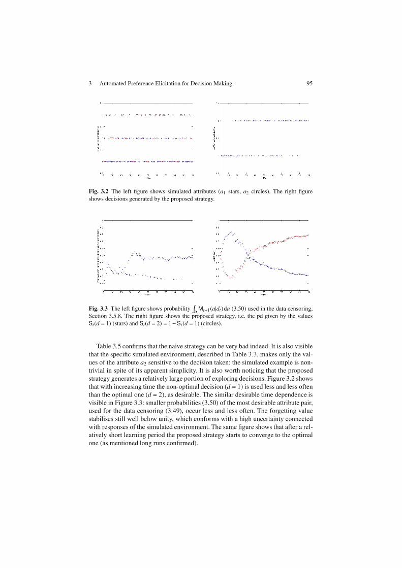
3 Automated Preference Elicitation for Decision Making 95
Fig. 3.2 The left figure shows simulated attributes (a1 stars, a2 circles). The right figure
shows decisions generated by the proposed strategy.
Fig. 3.3 The left figure shows probability∫
αααMt+1(a|dt)da (3.50) used in the data censoring,
Section 3.5.8. The right figure shows the proposed strategy, i.e. the pd given by the values
St(d = 1) (stars) and St(d = 2) = 1−St(d = 1) (circles).
Table 3.5 confirms that the naive strategy can be very bad indeed. It is also visible
that the specific simulated environment, described in Table 3.3, makes only the val-
ues of the attribute a2 sensitive to the decision taken: the simulated example is non-
trivial in spite of its apparent simplicity. It is also worth noticing that the proposed
strategy generates a relatively large portion of exploring decisions. Figure 3.2 shows
that with increasing time the non-optimal decision (d = 1) is used less and less often
than the optimal one (d = 2), as desirable. The similar desirable time dependence is
visible in Figure 3.3: smaller probabilities (3.50) of the most desirable attribute pair,
used for the data censoring (3.49), occur less and less often. The forgetting value
stabilises still well below unity, which conforms with a high uncertainty connected
with responses of the simulated environment. The same figure shows that after a rel-
atively short learning period the proposed strategy starts to converge to the optimal
one (as mentioned long runs confirmed).

96 M. Karny
3.7 Concluding Remarks
The chapter proposes a methodology of an automated elicitation of DM preference
when the set of the most desirable attribute values is specified. This specification is
quite common and can be extended to a preferential hierarchy with tunable weights
of the DM preferences.
Many important features of the proposed solution are implied by the fact that
the constructed ideal pd respects the relation between attributes and decisions as
described by the environment model Mt(a|d). Specifically,
• The proposed ideal pd is not fully concentrated on the most desirable attribute
value, which reflects that it cannot be reached with certainty.
• The functional form of the ideal pd is determined by the model Mt(a|d): it is not
created in an ad-hoc, model independent, manner unlike utilities [33].
• It is always possible to project the constructed ideal pd into a class of feasible pds
by using information criterion justified in [5], [28], Section 3.2, if the constructed
ideal pd is too complex for numerical treatment or analysis.
• The environment model Mt(a|d) as well as the closed-loop model with the opti-
mal strategy Pt(a,d)=Mt(a|d)st(d) are sequentially learnt; consequently, the DM
preference description given by the ideal pd It(a,d) derived from them, is learned,
too.
• The approach can be directly extended to a dynamic DM with a regression-type
dependence.
• The involved pds can quantify the joint distributions of discrete-valued and
continuous-valued attributes. This simplifies the elicitation of the DM prefer-
ences given by categorical as well as numerical attributes.
Suppression or a more firm justification of ad-hoc steps (e.g. choice of forgetting
factors in tracking of the changed DM preferences or in data censoring) is the key
methodological research direction. At a more practical level, covering other DM
preference specifications is the important problem to be addressed. The proposed
solution is clearly connected with the DM preference learning presented in [27].
There, an explicit dependence between the environment-model parameter and the
parameter of the optimal strategy has been established in a special, practically sig-
nificant, way. A more detailed and general inspection of this relation is another open
problem. The design of specific algorithmic solutions for commonly used environ-
ment models is a further topic to be covered.
In spite of the width of the problems hidden behind these open research direc-
tions, the proposed methodology appears practically promising.
Acknowledgements. This research and chapter have been strongly influenced by Dr. Ta-
tiana V. Guy who I take as co-author of innovative and interesting parts of this text. I do
acknowledge her help very much indeed.
The support of the project GACR 13-13502S is acknowledged. The support of the project
GACR 102/08/0567 is also acknowledged.

3 Automated Preference Elicitation for Decision Making 97
References
1. Abramowitz, M., Stegun, I.: Handbook of Mathematical Functions. Dover Publications,
New York (1972)
2. Barndorff-Nielsen, O.: Information and exponential families in statistical theory, New
York (1978)
3. Berec, L., Karny, M.: Identification of reality in Bayesian context. In: Warwick, K.,
Karny, M. (eds.) Computer-Intensive Methods in Control and Signal Processing: Curse
of Dimensionality, Birkhauser, Boston, pp. 181–193 (1997)
4. Berger, J.: Statistical Decision Theory and Bayesian Analysis. Springer, New York
(1985)
5. Bernardo, J.M.: Expected information as expected utility. The Annals of Statistics 7(3),
686–690 (1979)
6. Bohlin, T.: Interactive System Identification: Prospects and Pitfalls. Springer, New York
(1991)
7. Boutilier, C.: A POMDP formulation of preference elicitation problems. In: Biundo, S.
(ed.) AAAI-2002 Proc. of the Fifth European Conference on Planning, pp. 239–246.
AAAI Press, Durham (2002)
8. Boutilier, C., Brafman, R., Geib, C., Poole, D.: A constraint-based approach to prefer-
ence elicitation and decision making. In: Proceedings of AAAI Spring Symposium on
Qualitative Decision Theory, Stanford, CA, pp. 19–28 (1997)
9. Bowong, S., Dimi, J., Kamgang, J., Mbang, J., Tewa, J.: Survey of recent results of multi-
compartments intra-host models of malaria and HIV. Revue ARIMA 9, 85–107 (2008)
10. Chajewska, U., Koller, D.: Utilities as random variables: Density estimation and structure
discovery. In: Proceedings of UAI 2000, pp. 63–71 (2000)
11. Cooke, N.: Varieties of knowledge elicitation techniques. International Journal of
Human-Computer Studies 41, 801–849 (1994)
12. Feldbaum, A.: Theory of dual control. Autom. Remote Control 21(9) (1960)
13. Gajos, K., Weld, D.: Preference elicitation for interface optimization. In: Proceedings of
UIST 2005 (2005)
14. Garthwaite, P., Kadane, J., O´Hagan, A.: Statistical methods for eliciting probability dis-
tributions. J. of the American Statistical Association 100(470), 680–700 (2005)
15. Guy, T.V., Karny, M., Wolpert, D.H. (eds.): Decision Making with Imperfect Decision
Makers. ISRL, vol. 28. Springer, Heidelberg (2012)
16. Viappiani, H.P., Boutilier, S.Z., Learning, C.: complex concepts using crowdsourcing: A
Bayesian approach. In: Proceedings of the Second Conference on Algorithmic Decision
Theory (ADT 2011), Piscataway, NJ (2011)
17. Haykin, S.: Neural Networks: A Comprehensive Foundation. Macmillan, New York
(1994)
18. Horst, R., Tuy, H.: Global Optimization, p. 727. Springer (1996)
19. Jacobs, O., Patchell, J.: Caution and probing in stochastic control. Int. J. of Control 16,
189–199 (1972)
20. Jaynes, E.: Information theory and statistical mechanics. Physical Review Series
II 106(4), 620–630 (1957)
21. Jimison, H., Fagan, L., Shachter, R., Shortliffe, E.: Patient-specific explanation in models
of chronic disease. AI in Medicine 4, 191–205 (1992)
22. Jorgensen, S.B., Hangos, K.M.: Qualitative models as unifying modelling tool for grey
box modelling. Int. J. of Adaptive Control and Signal Processing 9(6), 461–562 (1995)
23. Karny, M.: Towards fully probabilistic control design. Automatica 32(12), 1719–1722
(1996)

98 M. Karny
24. Karny, M., Andrysek, J., Bodini, A., Guy, T., Kracık, J., Nedoma, P., Ruggeri, F.: Fully
probabilistic knowledge expression and incorporation. Tech. Rep. 8-10MI, CNR IMATI,
Milan (2008)
25. Karny, M., Andrysek, J., Bodini, A., Guy, T.V., Kracık, J., Ruggeri, F.: How to exploit
external model of data for parameter estimation? Int. J. of Adaptive Control and Signal
Processing 20(1), 41–50 (2006)
26. Karny, M., Bohm, J., Guy, T.V., Jirsa, L., Nagy, I., Nedoma, P., Tesar, L.: Optimized
Bayesian Dynamic Advising: Theory and Algorithms. Springer, London (2006)
27. Karny, M., Guy, T.: Preference elicitation in fully probabilistic design of decision strate-
gies. In: Proc. of the 49th IEEE Conference on Decision and Control. IEEE (2010)
28. Karny, M., Guy, T.V.: On Support of Imperfect Bayesian Participants. In: Guy, T.V.,
Karny, M., Wolpert, D.H. (eds.) Decision Making with Imperfect Decision Makers.
ISRL, vol. 28, pp. 29–56. Springer, Heidelberg (2012)
29. Karny, M., Guy, T.V.: Fully probabilistic control design. Systems & Control Let-
ters 55(4), 259–265 (2006)30. Karny, M., Halouskova, A., Bohm, J., Kulhavy, R., Nedoma, P.: Design of linear
quadratic adaptive control: Theory and algorithms for practice. Kybernetika 21(Supple-
ment to Nos. 3, 4 ,5, 6) (1985)
31. Karny, M., Kroupa, T.: Axiomatisation of fully probabilistic design. Information Sci-
ences 186(1), 105–113 (2012)
32. Karny, M., Kulhavy, R.: Structure determination of regression-type models for adaptive
prediction and control. In: Spall, J. (ed.) Bayesian Analysis of Time Series and Dynamic
Models. ch.12, Marcel Dekker, New York (1988)33. Keeney, R., Raiffa, H.: Decisions with Multiple Objectives: Preferences and Value Trade-
offs. JohnWiley and Sons Inc. (1976)34. Koopman, R.: On distributions admitting a sufficient statistic. Tran. of American Mathe-
matical Society 39, 399 (1936)
35. Kuhn, H., Tucker, A.: Nonlinear programming. In: Proc. of the 2nd Berkeley Sympo-
sium, pp. 481–492. University of California Press, Berkeley (1951)
36. Kulhavy, R.: Can we preserve the structure of recursive Bayesian estimation in a limited-
dimensional implementation? In: Helmke, U., Mennicken, R., Saurer, J. (eds.) Systems
and Networks: Mathematical Theory and Applications, vol. I, pp. 251–272. Akademie
Verlag, Berlin (1994)37. Kulhavy, R., Zarrop, M.B.: On a general concept of forgetting. Int. J. of Control 58(4),
905–924 (1993)
38. Kullback, S., Leibler, R.: On information and sufficiency. Annals of Mathematical Statis-
tics 22, 79–87 (1951)
39. Kumar, P.: A survey on some results in stochastic adaptive control. SIAM J. Control and
Applications 23, 399–409 (1985)
40. Lainiotis, D.: Partitioned estimation algorithms, i: Nonlinear estimation. Information
Sciences 7, 203–235 (1974)
41. Linden, G., Hanks, S., Lesh, N.: Interactive assessment of user preference models: The
automated travel assistant. In: Proceedings of User Modelling 1997 (1997)
42. Loeve, M.: Probability Theory. van Nostrand, Princeton (1962), Russian translation,
Moscow
43. Nagy, I., Suzdaleva, E., Karny, M., Mlynarova, T.: Bayesian estimation of dynamic finite
mixtures. Int. Journal of Adaptive Control and Signal Processing 25(9), 765–787 (2011)
44. Nelsen, R.: An Introduction to Copulas. Springer, New York (1999)
45. O’Hagan, A., Buck, C.E., Daneshkhah, A., Eiser, J.R., Garthwaite, P.H., Jenkinson, D.J.,
Oakley, J., Rakow, T.: Uncertain judgement: eliciting experts’ probabilities. John Wiley
& Sons (2006)

3 Automated Preference Elicitation for Decision Making 99
46. Osborne, M., Rubinstein, A.: A course in game theory. MIT Press (1994)
47. Peterka, V.: Bayesian system identification. In: Eykhoff, P. (ed.) Trends and Progress in
System Identification, pp. 239–304. Pergamon Press, Oxford (1981)
48. Rao, M.: Measure Theory and Integration. John Wiley, New York (1987)
49. Savage, L.: Foundations of Statistics. Wiley, New York (1954)
50. Shi, R., MacGregor, J.: Modelling of dynamic systems using latent variable and subspace
methods. J. of Chemometrics 14(5-6), 423–439 (2000)
51. Shore, J., Johnson, R.: Axiomatic derivation of the principle of maximum entropy and
the principle of minimum cross-entropy. IEEE Tran. on Information Theory 26(1), 26–37
(1980)
52. Si, J., Barto, A., Powell, W., Wunsch, D. (eds.): Handbook of Learning and Approximate
Dynamic Programming. Wiley-IEEE Press, Danvers (2004)
53. Sindelar, J., Vajda, I., Karny, M.: Stochastic control optimal in the Kullback sense.
Kybernetika 44(1), 53–60 (2008)
