chapter 2 frame localisation algorithm
TRANSCRIPT
27
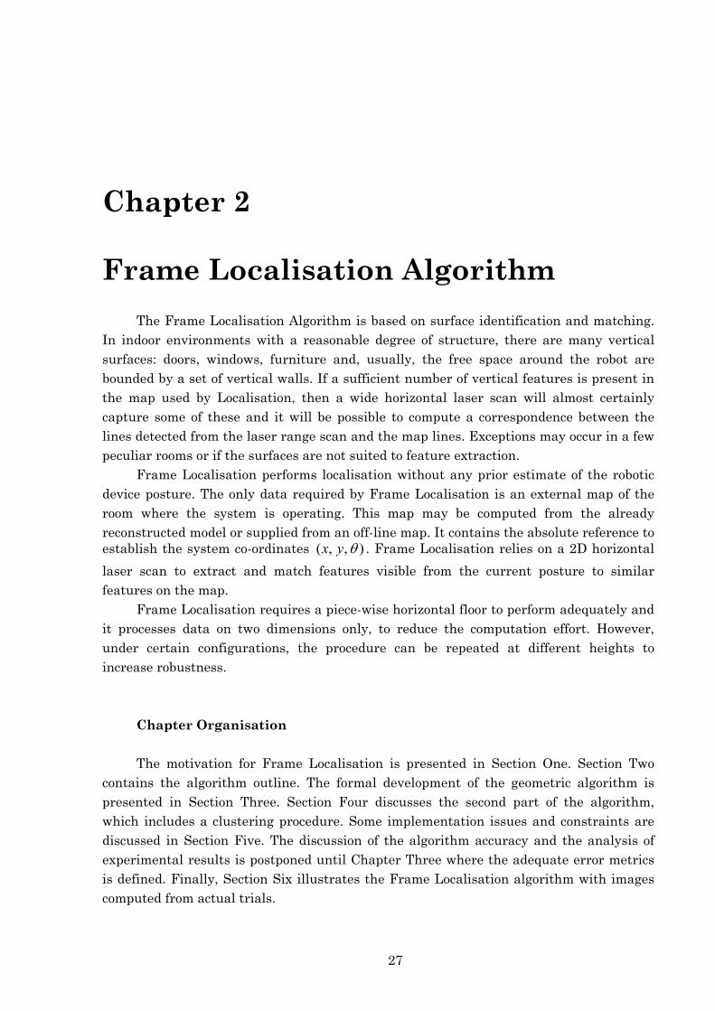
Chapter 2
Frame Localisation Algorithm The Frame Localisation Algorithm is based on surface identification and matching.
In indoor environments with a reasonable degree of structure, there are many vertical surfaces: doors, windows, furniture and, usually, the free space around the robot are bounded by a set of vertical walls. If a sufficient number of vertical features is present in the map used by Localisation, then a wide horizontal laser scan will almost certainly capture some of these and it will be possible to compute a correspondence between the lines detected from the laser range scan and the map lines. Exceptions may occur in a few peculiar rooms or if the surfaces are not suited to feature extraction.
Frame Localisation performs localisation without any prior estimate of the robotic device posture. The only data required by Frame Localisation is an external map of the room where the system is operating. This map may be computed from the already reconstructed model or supplied from an off-line map. It contains the absolute reference to establish the system co-ordinates ),,( θyx . Frame Localisation relies on a 2D horizontal
laser scan to extract and match features visible from the current posture to similar features on the map.
Frame Localisation requires a piece-wise horizontal floor to perform adequately and it processes data on two dimensions only, to reduce the computation effort. However, under certain configurations, the procedure can be repeated at different heights to increase robustness.
Chapter Organisation The motivation for Frame Localisation is presented in Section One. Section Two
contains the algorithm outline. The formal development of the geometric algorithm is presented in Section Three. Section Four discusses the second part of the algorithm, which includes a clustering procedure. Some implementation issues and constraints are discussed in Section Five. The discussion of the algorithm accuracy and the analysis of experimental results is postponed until Chapter Three where the adequate error metrics is defined. Finally, Section Six illustrates the Frame Localisation algorithm with images computed from actual trials.

28 2. FRAME LOCALISATION ALGORITHM
2.1 Motivation The localisation problem under study is stated as the computation of a planar 2D
position plus orientation posture ),,( θyx (Figure 1). The Frame Localisation requires a
two-dimension map and a planar laser-scan to compute the system (or robot) posture. This section introduces the method by use of a hypothetical environment being reconstructed by a robot equipped with the laser scanner only.
robot
x
yθ
Figure 1 – The co-ordinate system
Let’s assume a sample environment is being reconstructed as represented in Figure
2. The current map (Figure 3) encompasses only a fraction of it. This map is composed of planar curves, most often 2D lines, abbreviated as “map lines”. The map is often obtained from the reconstructed 3D model, but it can be provided from an off-line source like a 2D architectural plan. In Figure 4, the map is superimposed to the environment.
Figure 2 – The scene Figure 3 – The partial reconstructed
map Figure 4 – Map over
the scene The second element is the laser range scan. In order to compare the horizontal laser
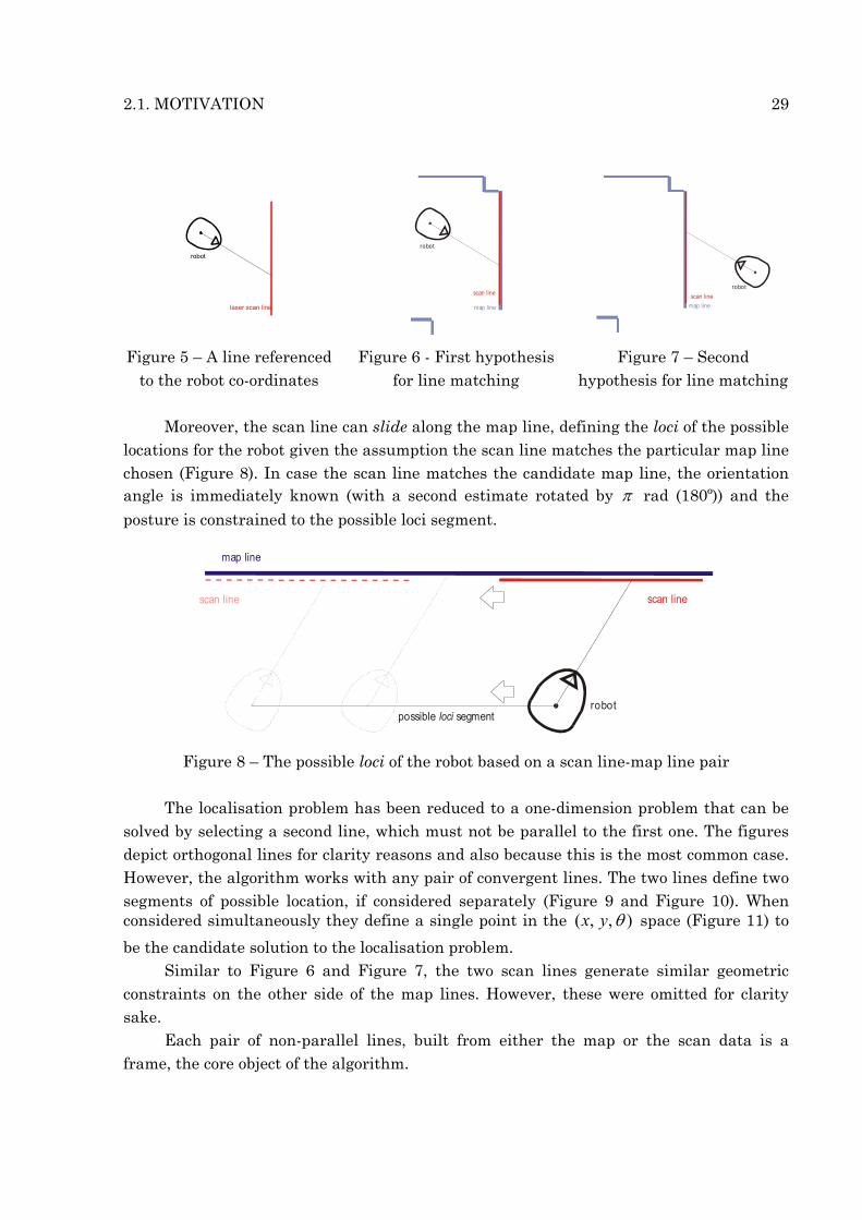
range data to the map, the range data is transformed in a set of planar curves, most often 2D lines. Each line is defined by its vertexes relative to the co-ordinate frame associated to the robot (Figure 5).
Because there is no auxiliary posture estimate, the line extracted from the laser range scan, abbreviated as “scan line”, can match any line on the environment, provided the length of the scan line is shorter than the map line. The scan line also matches the map line on the symmetric orientation (Figure 6 and Figure 7).
2.1. MOTIVATION 29
scan line
map line
robot
scan linemap line
robot
Figure 5 – A line referenced to the robot co-ordinates
Figure 6 - First hypothesis for line matching
Figure 7 – Second hypothesis for line matching
Moreover, the scan line can slide along the map line, defining the loci of the possible
locations for the robot given the assumption the scan line matches the particular map line chosen (Figure 8). In case the scan line matches the candidate map line, the orientation angle is immediately known (with a second estimate rotated by π rad (180º)) and the
posture is constrained to the possible loci segment.
map line
scan line scan line
possible segmentlocirobot
Figure 8 – The possible loci of the robot based on a scan line-map line pair The localisation problem has been reduced to a one-dimension problem that can be
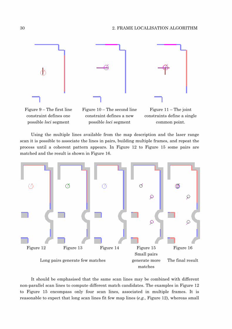
solved by selecting a second line, which must not be parallel to the first one. The figures depict orthogonal lines for clarity reasons and also because this is the most common case. However, the algorithm works with any pair of convergent lines. The two lines define two segments of possible location, if considered separately (Figure 9 and Figure 10). When considered simultaneously they define a single point in the ),,( θyx space (Figure 11) to
be the candidate solution to the localisation problem. Similar to Figure 6 and Figure 7, the two scan lines generate similar geometric
constraints on the other side of the map lines. However, these were omitted for clarity sake.
Each pair of non-parallel lines, built from either the map or the scan data is a frame, the core object of the algorithm.
30 2. FRAME LOCALISATION ALGORITHM
Figure 9 – The first line constraint defines one possible loci segment
Figure 10 – The second line constraint defines a new
possible loci segment
Figure 11 – The joint constraints define a single
common point. Using the multiple lines available from the map description and the laser range
scan it is possible to associate the lines in pairs, building multiple frames, and repeat the process until a coherent pattern appears. In Figure 12 to Figure 15 some pairs are matched and the result is shown in Figure 16.
Figure 12 Figure 13 Figure 14 Figure 15 Figure 16
Long pairs generate few matches Small pairs
generate more matches
The final result
It should be emphasised that the same scan lines may be combined with different
non-parallel scan lines to compute different match candidates. The examples in Figure 12 to Figure 15 encompass only four scan lines, associated in multiple frames. It is reasonable to expect that long scan lines fit few map lines (e.g., Figure 12), whereas small

2.1. MOTIVATION 31
lines fit different pairs of map lines (Figure 15). As Figure 16 shows clearly, the four different matches indicate a common ),,( θyx
posture and some spurious results due to environment symmetry; other spurious results laying outside the depicted area where the robot moves were suppressed for clarity reasons.
2.2 Frame Localisation Outline The Frame Localisation algorithm operation flow is illustrated in Figure 17, where
the operations represented by the shaded blocks, although necessary, are not strictly part of Frame Localisation. The algorithm starts with two lists of data, one from the map, the other evaluated from the horizontal laser range scan. The two lists are processed into a pair of new lists, the frame lists. Afterwards, a correspondence between compatible elements of both frame lists is established. The necessary condition for matching one scan frame to one map frame is that the scan frame axes fit within the map frame axes. For each successful match the co-ordinate transform is computed, producing a candidate posture estimate. Finally, all estimates are classified and sorted. The algorithm outcome is the possible posture list.
In order to validate the possible posture list, a simulated scan is computed as if the laser scanner was at each posture in the list and the result is compared with the real scan. On success, the postures are passed into the plausible posture list. This algorithm, depicted by the three shaded blocks, is described in Chapter 3.
plausibleposture list
possibleposture list
match compat ible
fr ames
compute robotto wor ld co-ordinate
transform
classify and sor t solut ions in
weighted cluster s
compute simulated scan from
environment map
extract lines from
laser range data
discard false solutions
compare laser scan to
simulated scan
scan line list map line list
build scan frame list
build map framelist
extract lines from
environment map
Figure 17 – Frame Localisation operation flow
32 2. FRAME LOCALISATION ALGORITHM
Frame Localisation is based on feature extraction and matching; the features currently extracted are straight lines, although the algorithm is compatible with other 2D curves, namely bi-quadratic. The RESOLV surface maps also implements bi-quadratic surfaces. The proposed extension was not implemented since the most environments have rich linear content and poor bi-quadratic content and this extension would increase significantly the computational burden.
A preliminary step of the algorithm is the extraction of the 2D profiles. The techniques used to create the map profiles depend on the type of map used. If
the map is obtained from the RESOLV’s 3D Reconstruction algorithms, the 2D map results from the intersection of the extracted 3D surfaces with a horizontal plane at height h, where h is the distance to the ground of the centre of rotation of the laser device. If the map is available beforehand, the data processing depends on the source data type. It may be the raw vertexes obtained from a paper plan marked on a digitizer table, the set of lines measured manually and put into a coherent frame, etc.. The methods used to translate the maps into the line lists are detailed in Appendix B.
The extraction of the line profiles from the laser data is a complex and delicate task if one wants to constrain the error propagation and, simultaneously, encompass the widest range of cases. It should be emphasised that the nature and statistics of the surfaces in the environment are unknown beforehand. All the issues mentioned in the Introduction (Section 1.4), about the laser errors contribute to degrade the raw data quality. In order to get some insight on the data statistics, the reflectance data is considered along with the range data.
The line extraction algorithm begins with an array of laser samples, representing a circular scan centred on the laser device. Each sample holds the distance from the laser to the nearest obstacle in the laser beam direction as well as the reflectance of the obstacle. The first step of the method is to split the wide-angle laser profile into a set of angular segments, using both range and reflectance data. Each segment contains a contiguous sets of points, describing one surface or multiple adjacent surfaces. Then, for each segment, the Least Square Estimation (LSE) is used to assert if the considered segment is a straight line. Restricting the analysis to straight lines simplifies the LSE procedure, which is implemented in an efficient iterative form, represented by six parameters only. The linear condition test is quite stringent. If the test succeeds, the segment is replaced by its vertexes; if the test fails, the segment is split in two. This is where the iterative form proves its benefits, since it suffices to compute the parameters for one of the sub-segments and subtract them from the whole segment parameters to get the two sub-segment parameters. The procedure is applied recursively until all the sub-segments are transformed into lines or they are small enough to be discarded. The final step of the algorithm is to merge the elementary line segments into longer segments.
The method is detailed and formalised in Appendix C.

2.2. FRAME LOCALISATION OUTLINE 33
Once the two sets of line segments are extracted from the laser range scan and the environment map, the line segments are grouped into geometric entities, hereinafter called frames. A frame is defined by two non-parallel line segments, named axes. The crossing point of the two axes, or their extensions, is the frame origin. In Figure 18, three frame examples are shown.
axis 2
axis 2
axis 2
axis 1origin
origin
origin
axis 1
axis 1 Figure 18 – Frame examples
The frame definition encompasses two types of variables: local parameters and
global reference variables. There are five local parameters (Figure 19): the start and end points of both axes, i.e., the distance from the origin to the start of the axis and the distance from the origin to the end of the axis, and the inner angle between the two axes, θ . The axis size, an important parameter in the subsequent computations, is readily available as 2211 , startendstartend −− . The local parameters are independent of the co-
ordinate system.
end
start1
start 2
end 2
1θ
frameorigin
Figure 19 – Frame local parameters The global variables define the origin’s posture (Figure 20): 2D position ),( yx and
heading or rotation, rθ , relative to the co-ordinate system associated to the line set: either
the map co-ordinates or the laser device co-ordinates. Assigning the heading, rθ , to axis 1
or 2 and to axis X or Y in the co-ordinate system is only a matter of convention, as long it is the same for all frames. The global variables relate the frame to its inertial co-ordinates system.
x
y
inertialcoordinatesystem
(x, y, )θr
θr
Figure 20 – Frame global variables

34 2. FRAME LOCALISATION ALGORITHM
Just like any other measured data, the laser scan data is affected by noise. An adequate model of the measurement noise propagated along the line extraction procedure seemed too complex. The range error on the measured data depends, by decreasing importance, on the nature and colour of the surface, the angle of incidence to the surface, the distance to the surface among other minor noise sources. The first condition is impossible to model beforehand. The second is very important if the incident laser beam is close to parallel with the surface and moderately important otherwise and the third depends on the laser device parameters.
Therefore, a heuristic criterion was developed to establish a scale of confidence on the laser scan frames, which is an attempt to encompass all these error factors. From the line extraction procedure, described in detail in Appendix C, results that the smaller line segments are poorly extracted because they are usually based on a very small number of samples. This fact induced a confidence criterion based on the size of the axis: the longer the axis, the higher the confidence level. A second criterion considered the reflectance of the points in the line segment to reflect the importance of the nature and colour of the surface. The third element of the confidence criterion describes the range measurement error as a function of the range. This is to be adjusted by the operator based on the laser technical specifications.
In a similar way, one could discuss about the influence of the noise embedded in the map representation, especially when it results from the 3D reconstruction algorithms, also based on laser data. However, since the map is the only available reference, it is regarded as the best possible representation of the environment.
The association of scan frames with suitable map frames is the core of the algo-
rithm. However, since the algorithm is intrinsically exponential a lot of effort was put in designing constraints to cope with its nature. The line sets are sorted by decreasing size, the frames are also sorted by decreasing size of their longer axis and the computations are performed iteratively until a coherent pattern occurs in the possible posture list.
To test whether one scan frame is a candidate match to a specific map frame requires only the local parameters. If the scan frame’s local parameters fit within the boundaries of the map frame’s local parameters (Figure 21) the two frames match. This is usually the case since the room profile perceived by the laser is a fraction of the total environment and many surfaces will be partially scanned, providing smaller lines than the original surface description.
Map
start1
start 2
end 2
end 1 θ
start1
start 2
end 2
end1
θ
Scan
Figure 21 – Frame match
2.2. FRAME LOCALISATION OUTLINE 35
Although it is conceivable that a smaller map frame may fit a larger scan frame, this will be seldom the case. On the other hand, this constraint reduces enormously the computation burden.
To compute the possible posture the global variables are used. Assuming the two frame origins are the same point and the frame axes share a common orientation, the origin postures are used to translate the local co-ordinates (used in the scan frames) to the map co-ordinates.
Naturally, it will occur often that one given scan frame fits a few map frames, as illustrated in the previous section. Therefore, the procedure must be repeated with a sufficient number of frames until a coherent pattern occurs in the solution space. Each candidate solution has its own weight, associated to the confidence criterion designed for the scan frames.
When the frame matching procedure is over, the result is a cloud of points ),,( ryx θ
and their associated weights in the posture space. All these posture points are then grouped into a few clusters. Each cluster congregates all points lying within a predefined range. Although this clustering procedure is clearly a crude solution, it proved adequate to this problem where there is a large and unknown number of clusters, clearly isolated from their neighbours. The posture points within each cluster are then replaced by an equivalent posture computed from the weighed average of all posture points in the cluster.
To enhance the clustering process, the isolated points (the "dust") are swept out of the posture set. After this, the ),,( ryx θ space shows only the cluster equivalents.
Usually, there is one solution with a confidence level much higher than all other solutions. This is the correct solution. The other points correspond to postures that meet some symmetry in the environment map.
The Frame Localisation concludes by listing all the possible postures by decreasing weight. To verify the correction of the proposed solution, the Likelihood Test was developed and it will be discussed in the next Chapter.
2.3 Formal Development
2.3.1 Frame generation The basic data element for frame definition is the line. The line il in equation (2.1)
(Figure 22), is defined by its vertexes, iv1 and iv2 , referred to the appropriate co-ordinate
frame. The map lines are referred to the environment inertial reference and the scan lines are referred to the sensor head axis where the laser is mounted, or equivalently, to the robot co-ordinate reference.

36 2. FRAME LOCALISATION ALGORITHM
))(,)(()()()()(
),(),(
),,(
1212
212
212
222
111
21
iiii
ii
ii
ii
iiiii
xxyyarctan2lyyxxldd
yxvyxv
wheredvvll
−−==
−+−==
==
→=
γγ
γ
(2.1)
y2i
di
y1i
x1ix2i
γj
Figure 22 – Line definition
For computational efficiency purposes, the line definition also contains the line size,
id , and orientation, iγ , referred to the robot co-ordinates, for the scan lines and to the
world co-ordinates for the map lines. The immediate access to the line size and orientation is an essential element to the efficiency of the algorithm, as it will be shown in the next sections.
The data available to Frame Localisation are two line lists, sorted by decreasing size. The map list and the scan list are denoted by M and S, where M is the list of all the lines extracted from the map and S is the list of all the lines extracted from the laser range scan:
List of Map lines, M: { }l M d l d li i i∈ > +: ( ) ( )1
List of Scan lines, S: { }l S d l d lm m m∈ > +: ( ) ( )1
A frame results from joining a pair of non-parallel lines from the same list. A pre-
defined threshold, NPθ , is used to decide whether the two lines are parallel1 or not. Each
line is termed an axis of the frame. The generic frame ijf results from lines il and jl .
The first parameter on the frame to be computed is the inner angle, innerθ , computed
directly from the definition – equation (2.2). If the inner angle complies with the non-parallel restriction - equation (2.3) - the computations associated to the axes size and the origin posture are performed, otherwise that pair is discarded and a new pair of candidate lines is considered.
1 The tuning of θ NP is not critical. In most cases the frame axis are nearly orthogonal and frame computations are very stable if the inner angle is above 0.05 rad (3º).
2.3. FORMAL DEVELOPMENT 37
θ γ γinner i j= − , reduced to the interval [0, π[ (2.2)
θ θinner NP≥ (2.3)
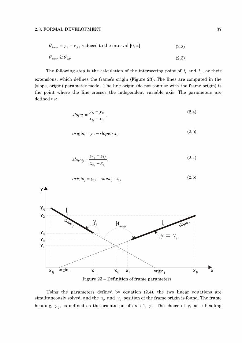
The following step is the calculation of the intersecting point of il and jl , or their
extensions, which defines the frame’s origin (Figure 23). The lines are computed in the (slope, origin) parameter model. The line origin (do not confuse with the frame origin) is the point where the line crosses the independent variable axis. The parameters are defined as:
jjjj
jj
jjj
iiii
ii
iii
xslopeyorigin
xxyy
slope
xslopeyorigin
xxyy
slope
11
12
12
11
12
12
;
;
⋅−=
−
−=
⋅−=
−−
=
(2.4)
(2.5)
(2.4)
(2.5)
y2i
y1i
yij
y1j
y2j
x1ix1j xijorigin i
slope islope j
origin j x2ix2j
γ γi ij=
γj θinnerli
lj
y
x
Figure 23 – Definition of frame parameters Using the parameters defined by equation (2.4), the two linear equations are
simultaneously solved, and the ijx and ijy position of the frame origin is found. The frame
heading, ijγ , is defined as the orientation of axis 1, 1γ . The choice of 1γ as a heading
38 2. FRAME LOCALISATION ALGORITHM
reference is arbitrary, provided the convention is the same for all frames. Equations (2.6) define the frame global parameters, relating the frame to its co-ordinate system.
=
⋅+=
−
−−=
1γγ ij
iiij
ij
ijij
ijxslopeoriginy
slopeslopeoriginorigin
x
(2.6)
If one of the axes is nearly vertical, equation (2.4) is not valid. It would be possible to
use an alternative parametric definition of a line ( r x y= ⋅ + ⋅cos( ) sin( )α α ) to avoid the
singularity near the vertical. However, the former representation was kept because the slope is readily available from the axis orientation, ( slope = tan( )γ ), and the computations
are much faster. In case the axis i, for instance, is nearly vertical, equations (2.4) and (2.6) are replaced by:
1ij
ijij
21
2
γγ =
⋅+=
+=
xslopeoriginy
xxx
jj
iiij
(2.7) substitutes (2.4)
(2.8) substitutes (2.6)
while equations (2.4) and (2.5) hold. The overall result, including the vertical axis exception handling, although less straightforward, is very efficient. At the same time, the distances of the axis’s vertexes to the frame origin are computed (Figure 19),
2ij2
2ij22
2ij1
2ij12
2ij2
2ij21
2ij1
2ij11
)()()()(
)()()()(
yyxxendyyxxstart
yyxxendyyxxstart
jjjj
iiii
−+−=−+−=
−+−=−+−=
(2.9)
concluding the definition of the local parameters. In equations (2.4) to (2.9), the xy-co-ordinates are defined in the line co-ordinate system, either the robot or the world reference.
It should be noticed that the origin parameters of frame ijf , generated by il for axis
2.3. FORMAL DEVELOPMENT 39
1 and jl for axis 2 is different from those of frame jif , generated by jl for axis 1 and il
for axis 2: their headings are symmetric. However, no confusion arise since only one of them is present in the frame set, as it will be shown below.
In summary, a frame is defined by five local parameters: start and end of the two axis and the inner angle ),,,,( 2211 innerendstartendstart θ , which are independent of a
external reference, and three global parameters relative to a fixed reference, which define the frame origin posture ),,( ijijij yx γ . The laser scan frames are based on the robot co-
ordinate system and the map frames are based on the world co-ordinate system. The computation of the two frame sets follows directly from the frame definition. As
already discussed and for computational efficiency reasons, only the lines that are long enough are added to the frame sets. However, a long line may be “framed” with a small line, providing a reliable feature. Thus, two parameters exist for the minimum size:
longlim for the longer axis and smalllim for the shorter one. The frame ijf is a member of
the frame set F, if the four conditions are simultaneously satisfied:
>−>><
∈
NPji
smallj
longiij limld
limldji
iffFf
θγγ)()(
(2.10)
The two frame sets are then sorted according to the axis sizes to enhance the
computational efficiency: for each frame, the two axis sizes are measured and the longest is used to sort the list. The two frame lists are derived from the two line lists (either the map list or the scan list), using a combination of any lines, il and jl , abiding to the non-
parallel constraint defined by equation (2.3). The only difference between frame fij and
frame f ji is the inner angle, innerθ . Thus, only the first is stored and the frame match
procedure will test for both angles. Also, iif doesn’t exist since a line is parallel to itself. In
conclusion, all frames in a list abide to the f i jij : < constraint. The sorting criterion
reduces the frame list to half of the possible combinations and optimises the frame matching procedure, as it will be shown in the next section.
In many cases, the lines are grouped into two main directions, corresponding to
square angles environments. In such environments, one of the directions is termed horizontal, while the other is vertical, H and V respectively, regardless of the robot’ alignment with any of these. Under these conventions, both frame lists may be presented as a table of a hypothetical frame set:

40 2. FRAME LOCALISATION ALGORITHM
f frame l l f frame l l f frame l l f frame l lf frame l l f frame l l f frame l l f frame l lf frame l l f frame l lf frame l l f frame l l f frame l l
v h v h v h v h
v h v h v h v h
h v h v
v h v h v
1 1 1 2 1 2 3 1 3 4 1 4
5 2 1 6 2 2 7 2 3 6 2 4
9 1 3 10 1 4
11 3 2 12 3 3 13 3 4
= = = == = = == == = =
( , ) ( , ) ( , ) ( , ) .. .( , ) ( , ) ( , ) ( , ) .. .( , ) ( , ) .. .( , ) ( , ) ( , h
h v
h v
h v
f frame l lf frame l lf frame l l
) .. .( , ) . . .( , ) . . .( , ) . . .
. . .
14 2 4
15 3 4
16 4 4
===
(2.11)
In equation (2.11), the first elements of the frame list are presented, assuming the
following line order2: l l l l l l l lv v h v h h h v1 2 1 3 2 3 4 4, , , , , , , , ... , where ivl is the i-th vertical line and jhl
is the j-th horizontal line. The )(frame function embodies the frame generation procedure. The frame numbering no longer follows the previous indexing convention ( fij ).
Instead, a new frame list order is defined by the decreasing size of the longer axis. This form emphasises the concern of how to cope with the intrinsic exponential character of the algorithm. Although the number of possible frames generated by small line lists is apparently huge, the design reduces the number of frames to a fraction of it. Moreover, the design is incremental: if a given number of frames are insufficient to compute an accurate solution, the frame sets may be extended without re-computing any of the existing frames.
2.3.2 Frame matching Once the two frame lists - or equivalently frame table, using the form in equation
(2.11) - are defined, the matching algorithm initiates. One frame table is fixed, the map frame table, for instance. Then, each element of the other frame table - in this case, the scan frame table - is compared to each candidate on the fixed table.
The match test conditions are expressed in equation (2.12) and must be met simultaneously. Figure 21 - repeated on the left of Figure 24 - illustrates a successful frame match case.
start start end end
start start end end
Mapm
Scan Scan Mapm
Mapm
Scan Scan Mapm
Mapang
Scan Mapang
1 1 1 1
2 2 21 2
− ≤ < ≤ +
− ≤ < ≤ +
− ≤ ≤ +
δ δ
δ δ
θ δ θ θ δ
(2.12)
Equation (2.12) uses the map table as the “fixed” element and the scan frame as the
frame under test. The axis length tolerance is defined by mδ ; angδ defines the angle
tolerance. Each pair of frames is tested twice, because the assignment of axis 1 and axis 2
2 The lines are sorted by decreasing size, no matter their relative orientation.
2.3. FORMAL DEVELOPMENT 41
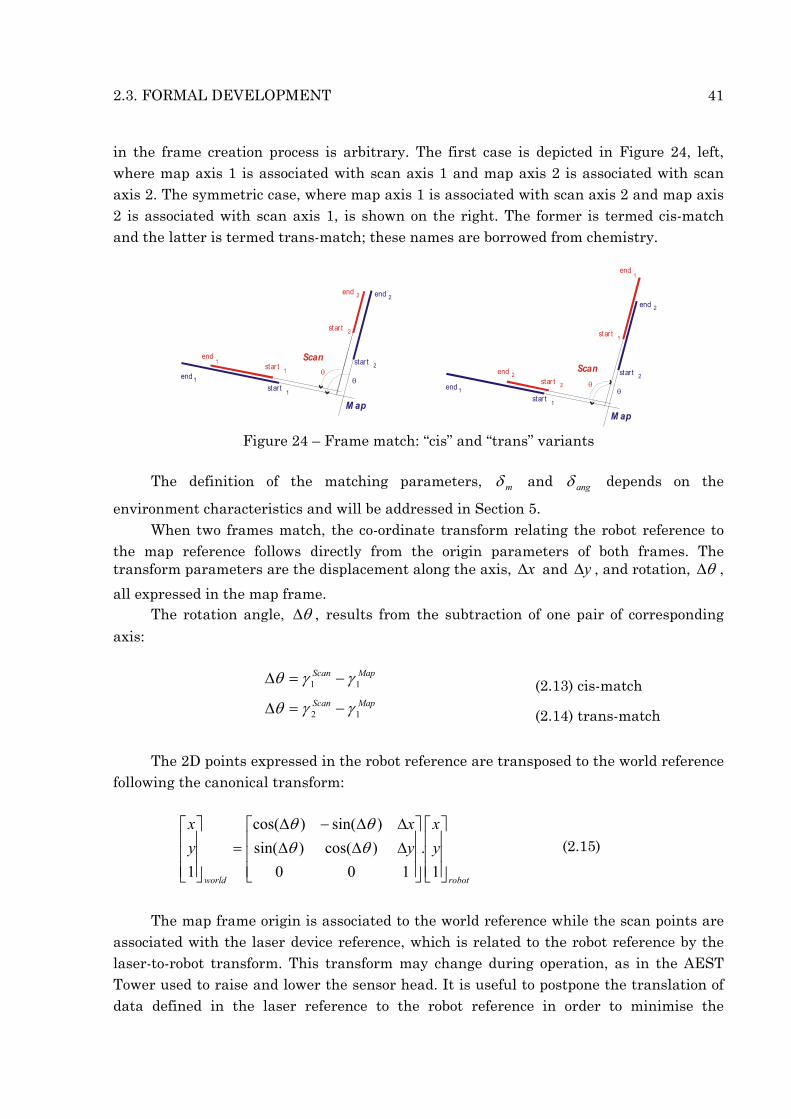
in the frame creation process is arbitrary. The first case is depicted in Figure 24, left, where map axis 1 is associated with scan axis 1 and map axis 2 is associated with scan axis 2. The symmetric case, where map axis 1 is associated with scan axis 2 and map axis 2 is associated with scan axis 1, is shown on the right. The former is termed cis-match and the latter is termed trans-match; these names are borrowed from chemistry.
star t 1
star t 2
end 2
end1
θstar t 2
end 2
star t 1
end1
θstar t 1
star t 2
end 2
end 1 θ
star t 1
star t 2
end 2
end 1 θ
M apM ap
ScanScan
Figure 24 – Frame match: “cis” and “trans” variants
The definition of the matching parameters, mδ and angδ depends on the
environment characteristics and will be addressed in Section 5. When two frames match, the co-ordinate transform relating the robot reference to
the map reference follows directly from the origin parameters of both frames. The transform parameters are the displacement along the axis, x∆ and y∆ , and rotation, θ∆ ,
all expressed in the map frame. The rotation angle, θ∆ , results from the subtraction of one pair of corresponding
axis:
MapScan11 γγθ −=∆ (2.13) cis-match MapScan12 γγθ −=∆ (2.14) trans-match
The 2D points expressed in the robot reference are transposed to the world reference
following the canonical transform:
robotworld
yx
yx
yx
∆∆∆∆∆−∆
=
1.
100)cos()sin()sin()cos(
1θθθθ
(2.15)
The map frame origin is associated to the world reference while the scan points are
associated with the laser device reference, which is related to the robot reference by the laser-to-robot transform. This transform may change during operation, as in the AEST Tower used to raise and lower the sensor head. It is useful to postpone the translation of data defined in the laser reference to the robot reference in order to minimise the

42 2. FRAME LOCALISATION ALGORITHM
computational burden. Thus, the evaluated postures describe the location of the laser sensor origin. Only at the end of the Localisation algorithms, the unique resulting posture will be translated to the actual robot location.
Choosing the origins of both frames as candidate points and solving with respect to x∆ and y∆ , yields:
ScanMap
yx
yx
yx
∆∆∆−∆
−
=
∆∆
1.
1000)cos()sin(0)sin()cos(
10θθθθ
(2.16)
The three resulting figures represent both the transform parameters between
references and the posture of the laser sensor with respect to the environment map:
ScanMap yxyx ),,(),,( θθ ⇔∆∆∆ . (2.17)
At this stage, a candidate posture is fully defined.
2.4 Candidate posture clustering Iterating the matching procedures for all possible candidates generates a cloud of
postures in the ),,( θyx space. Each point in a cloud records one frame match and, as
already discussed, it has an associated weight, which corresponds to a degree of confidence assigned to each particular result. The weighting criterion is based on the size of the axis. It uses the product of the axis size to minimise the influence of small lines and maximise the influence of large, balanced frames.
Given a cloud of N posture points in the ),,( θyx space, each corresponding to a
candidate posture, the weight of the i-th point, iw , is defined in equation (2.18), where
1size and 2size refer to the scan frame axes length. The weight is added to the posture
generating a 4-parameter point, ip , defined in equation (2.19).
w size sizei
Scan Scan= 1 2. (2.18)
Ni
w
yx
p
i
i
i
i
i ,...,1,0, =
=θ
(2.19)
The clustering algorithm was kept very simple at the expense of some loss of
generality. This implementation suits the type of clustering problem: i) a large and
2.4. CANDIDATE POSTURE CLUSTERING 43
unknown number of clusters, ii) the distance between neighbours in the same cluster is much smaller than the distance between neighbouring clusters. A sounder algorithm, from which the present one derives, was implemented but the results were very similar at the expense of a larger computational effort. This algorithm is presented in Appendix D.
The cluster definition is similar to the point definition, equation (2.20).
,...1,0, =
= j
w
yx
c
clj
clj
clj
clj
j θ
(2.20)
The clustering algorithm is based on the following rules:
1. The first point, 1p , is the seed of the first cluster 1c .
2. The set of equations (2.21) defines the radius of the cluster. Hence, the angular distance between candidate ip and cluster jc must be closer than angledif and the
linear distance from ip to jc must be closer than centdif . The two parameters, angledif
and centdif , are fixed beforehand. If the two conditions are satisfied ip is added to the
cluster jc according to equation (2.22), a weighed sum that updates the cluster
posture. The total cluster weight is updated according to equation (2.23). If ip fails the
(2.21) test for every cluster then ip initiates a new cluster.
3. The algorithm repeats until the N points are tested.
<−+−
<−
centclji
clji
angleclji
difyyxx
dif
22 )()(
θθ
(2.21)
+
+=
+
+=
+
+=
iclj
iiclj
cljcl
j
iclj
iiclj
cljcl
j
iclj
iiclj
cljcl
j
wwwwwwywyw
y
wwxwxw
x
θθθ
..
..
..
(2.22)
iclj
clj www += (2.23)

44 2. FRAME LOCALISATION ALGORITHM
The result of the clustering process is a set of C clusters in the form of equation (2.20). The cluster list is sorted by decreasing weights and the result is the possible posture list, which concludes the Frame Localisation Algorithm.
2.4.1 Selection of best candidate posture
The solutions included in the possible posture list were computed regarding only a small fraction of the environment. In fact, each individual candidate is based on one single frame, or equivalently, two surfaces only. Considering the posture candidates aggregated in clusters, the relative confidence is enhanced in the most “heavy” clusters since they embrace a wider fraction of the scene, containing multiple surfaces.
Therefore, the final operations of the Frame Localisation deal with the possible posture list. The single elements, i.e., the candidate postures that were not corroborated by other surface matches, i.e., clusters with a single element are discarded, no matter their weight. The clusters representing the candidate solutions are sorted by decreasing weight. In order to make the result interpretation clear to the human operator, the cluster weights are normalised, adding up to a total weight of 1.0.
At the end of Frame Localisation, the proposed postures were not yet tested in a thorough match between the whole scan and the available map. This is the task of the performance evaluation statistics, termed Likelihood Test, which is the object of the next chapter.
2.5 Implementation Issues Along the chapter, several parameters were mentioned with little details. In
addition, some technicalities were not mentioned to minimise the overhead in the explanation of the core of the algorithm. This section discusses these issues.
2.5.1 Line representation and frame building
The line representation aims at maximum efficiency and robustness at the cost of some redundancy and notational compactness. The (slope, origin) parameter model (2.24) was adopted since it involves no trigonometric computations, which are usually time-consuming and copes with the singularity near the vertical with an if condition.
For the sake of numerical stability and mathematical aesthetics, an enhanced variant for line intersection was implemented. If the slope is high, a small error sδ in the
slope estimate multiplies the error into the co-ordinate estimates (2.25) (see also (2.6)).
xslopeoriginy kk ⋅+= (2.24)
2.5. IMPLEMENTATION ISSUES 45
xslopeyxslopeorigin skskk ⋅⋅+=⋅+⋅+ δδ )1( (2.25)
Instead of considering an exception near the vertical slope, the slope-space was split
in two symmetric modes: in mode X the line is defined as )(xy (2.26) and in mode Y it is defined by )(yx (2.27). This approach minimises the slope error and simultaneously
handles the singularity near the vertical: Mode X xslopeoriginxy X
kXk ⋅+=)( (2.26)
Mode Y yslopeoriginyx Yk
Yk ⋅+=)( (2.27)
The transformation of a given (slope, origin) pair to the other mode is trivial from
the vertex definition given by (2.4) and (2.5). Notwithstanding, the line definition, including the vertex definition, is re-initialised, taking advantage of the iterative approach used for the line extraction (see Appendix C).
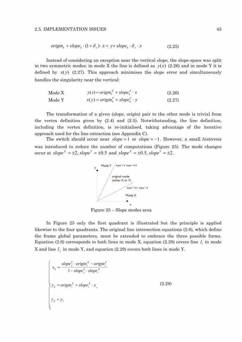
The switch should occur near 1=slope or 1−=slope . However, a small histeresis
was introduced to reduce the number of computations (Figure 25). The mode changes occur at 5.0,2 ±=±= YX slopeslope and 2,5.0 ±=±= YX slopeslope .
y
x
Mode X
Mode Y
original mode(either X or Y)
slope =2 slope =0.5X Y
slope =0.5 slope =2X Y
Figure 25 – Slope modes area
In Figure 25 only the first quadrant is illustrated but the principle is applied
likewise to the four quadrants. The original line intersection equations (2.6), which define the frame global parameters, must be extended to embrace the three possible forms. Equation (2.6) corresponds to both lines in mode X, equation (2.28) covers line il in mode
X and line jl in mode Y, and equation (2.29) covers both lines in mode Y.
=
⋅+=
⋅−
−⋅=
1
1
γγ ij
Xi
Xiij
Xi
Yj
Yj
Xi
Yj
ij
ijxslopeoriginy
slopeslopeoriginoriginslope
x
(2.28)
46 2. FRAME LOCALISATION ALGORITHM
=
⋅+=
−
−−=
1γγ ij
Yi
Yiij
Yj
Yj
Yi
Yj
ij
ijyslopeoriginx
slopeslopeoriginorigin
y
(2.29)
Obviously, the local parameters are also adjusted as a result of the redefinition of
the line parameters. The new definition reduces the influence of the line extraction process into the
frame definition, especially when the two lines in the frame are far apart. It should be noticed that the inner angle constraint (2.3) protects the frame definition equations - (2.6), (2.28) and (2.29) - from singularity. If the two slopes are very close, equation (2.3) will fail. In equation (2.28) singularities occur when one slope is close to the inverse of the other. However, since they are defined in opposite modes this corresponds to almost parallel lines.
2.5.2 The influence of the Laser errors The most important source of measurement errors is the target surface. Depending
on the colour and the texture of the surface the laser can receive an accurate measure, a wrong measure or no measure at all. The remaining error sources are, by decreasing importance, the incidence angle of the laser beam on the surface, the range measurement as a function of the range and other minor sources, such as the mechanical errors of the sensor.
Thus, it seemed inadequate to create a covariance matrix associated to each of the variables as in [ArrasK]. Instead, intensive experiments were carried out to have some insight about the data statistics, as if the sensor was a black box. The experiments confirmed the dominance of the colour and nature of the target surface over the remaining error factors. The results provide little information about the statistics, compared to the type of information conveyed in the formal covariance definition. Notwithstanding, some conclusions may be extracted:
• The reflectance data is of paramount importance to validate the range data. • The reflectance depends on the colour and on the texture of the surface, and the
two factors have comparable importance. • The average range error increases as the reflectance decreases. However, the
range measures degrade for high reflectivity surfaces too. This is a characteristic of each laser device.

2.5. IMPLEMENTATION ISSUES 47
• The repeatability of the range measurements degrades in face of poor reflectance surfaces. This effect can be detected by oversampling.
• The range samples in presence of glass and mirrored surfaces induce large variations in the range and reflectance values among adjacent samples.
• The integration time3 of the laser is of little importance above a given threshold specified by the laser manufacturer.
Given these conclusions, a confidence measure was associated to each sample, based
on its reflectance. The relation between the laser range error for each sample and the associated reflectance is again a matter of heuristics. In general terms, below a given threshold the range measurements are unreliable. As the reflectance increases, the confidence level also increases until a second threshold is attained. Above that, increased reflectance means decreasing confidence. This is usually the case with very reflective surfaces such as metal file cabinets and polished aluminium, used often in office environments. In case the reflectance is close to the maximum value, the confidence level is fixed because the reflectance data changes from sample to sample within the specified interval preventing any detailed analysis of the variations.
The coding of the reflectance is specific to each laser device. For the lasers used in the RESOLV project, it is an integer variable with 64 or 128 steps between no reflectance data and maximum reflectance. There is also a flag to indicate read failure. In Figure 26, it is presented a possible confidence curve according to the heuristic criterion explained.
negligibleconfidence
confidence
reflectance
decreasingconfidence
optimalconfidence
1.0
0.0
Figure 26 - Confidence value depending on the reflectance The detection of glass and mirrored surfaces is a complex issue, involved in more
heuristics. According to the experiments, a high quality mirror close to the laser device is very hard to detect. It behaves like a “window” to a virtual scene, a conical and expanded copy of the surrounding scene. When the mirror is at a greater distance, it may occur that the total distance exceeds the laser operation range and the results exhibit a low
3 The integration time is the time the laser fires short light impulses at the target. The longer it is the higher the energy sent to the target and the data oversampling.
48 2. FRAME LOCALISATION ALGORITHM
confidence or they are invalid. The odd surfaces, especially partial mirrored windows, are detected with a criterion
based on simultaneous analysis of range and reflectance variation. This criterion is used for all surfaces, but the parameters aim particularly at the detection of windows, a very common problem with reconstruction of in-door scenes. Other common problems are the objects to small too be perceived by the sampling grid, such as in-door plants, pens and pencils on top of tables, etc..
Table 1 introduces this criterion with some sample surfaces. The confidence level decreases as the shading increases. To minimise the misjudgements the rule thresholds are not sharp. Instead, they define a fuzzy rule to change the confidence associated to each set of samples, and very few range samples are eliminated prior to the line extraction algorithms.
Low range variation High range variation
Low reflectance variation between adjacent samples
Regular surface Unknown
High reflectance variation between adjacent samples
An object on the wall (e.g. a picture or a poster)
A window, a curtain or a window blind
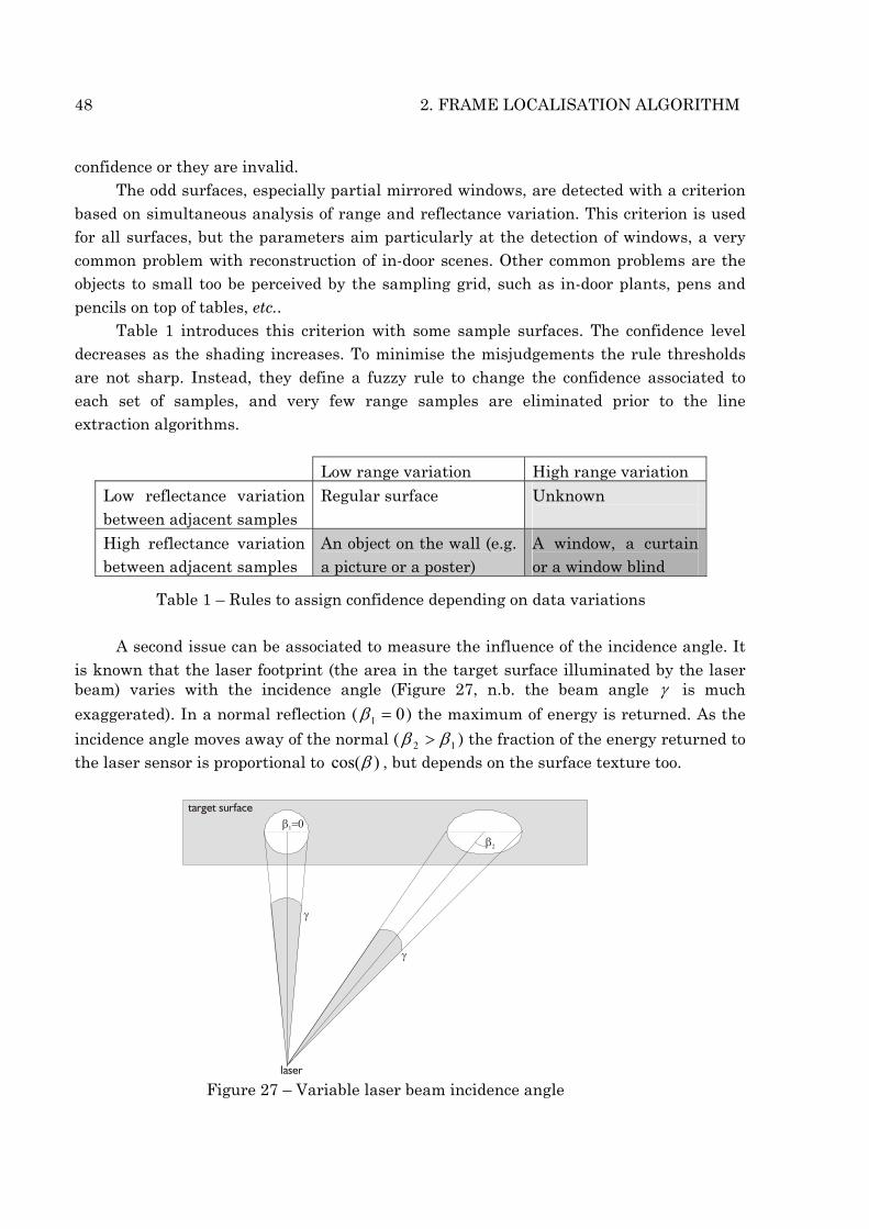
Table 1 – Rules to assign confidence depending on data variations A second issue can be associated to measure the influence of the incidence angle. It
is known that the laser footprint (the area in the target surface illuminated by the laser beam) varies with the incidence angle (Figure 27, n.b. the beam angle γ is much
exaggerated). In a normal reflection ( 01 =β ) the maximum of energy is returned. As the
incidence angle moves away of the normal ( 12 ββ > ) the fraction of the energy returned to the laser sensor is proportional to )cos(β , but depends on the surface texture too.
γ
γ
laser
target surfaceβ =01
β2
Figure 27 – Variable laser beam incidence angle
2.5. IMPLEMENTATION ISSUES 49
It would be possible to reprocess the reflectance data after the line extraction taking into account the corrected reflectance. However, this correction is negligible compared to the previous error causes and the computation burden would be significant. It should be noticed that for incidences from 0 to 4/π (30º) the correction would be of 13%. If the an-gle is high ( 4/πβ > , (45º)), the reflectance is reduced further and the confidence analysis
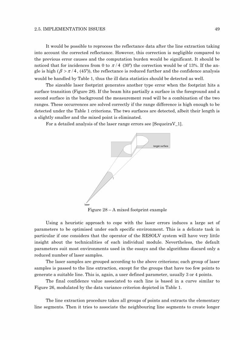
would be handled by Table 1, thus the ill data statistics should be detected as well. The sizeable laser footprint generates another type error when the footprint hits a
surface transition (Figure 28). If the beam hits partially a surface in the foreground and a second surface in the background the measurement read will be a combination of the two ranges. These occurrences are solved correctly if the range difference is high enough to be detected under the Table 1 criterions. The two surfaces are detected, albeit their length is a slightly smaller and the mixed point is eliminated.
For a detailed analysis of the laser range errors see [SequeiraV_1].
γ
laser
target surface
Figure 28 – A mixed footprint example
Using a heuristic approach to cope with the laser errors induces a large set of
parameters to be optimised under each specific environment. This is a delicate task in particular if one considers that the operator of the RESOLV system will have very little insight about the technicalities of each individual module. Nevertheless, the default parameters suit most environments used in the essays and the algorithms discard only a reduced number of laser samples.
The laser samples are grouped according to the above criterions; each group of laser samples is passed to the line extraction, except for the groups that have too few points to generate a suitable line. This is, again, a user defined parameter, usually 3 or 4 points. The final confidence value associated to each line is based in a curve similar to Figure 26, modulated by the data variance criterion depicted in Table 1.
The line extraction procedure takes all groups of points and extracts the elementary
line segments. Then it tries to associate the neighbouring line segments to create longer
50 2. FRAME LOCALISATION ALGORITHM
lines. In this process the individual confidence associated to each point group is merged into a single value, applied to each line. For more details, see Appendix C.
2.5.3 Representation of sets: line lists and frame lists It was explained before (Section 2) that the Frame Localisation algorithm is
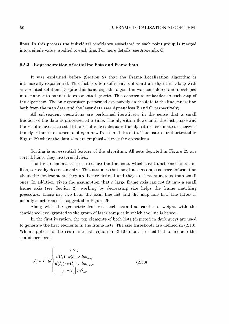
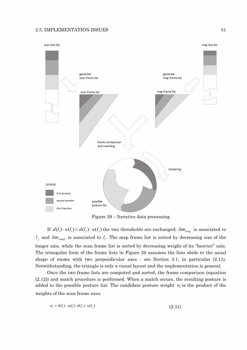
intrinsically exponential. This fact is often sufficient to discard an algorithm along with any related solution. Despite this handicap, the algorithm was considered and developed in a manner to handle its exponential growth. This concern is embedded in each step of the algorithm. The only operation performed extensively on the data is the line generation both from the map data and the laser data (see Appendices B and C, respectively). All subsequent operations are performed iteratively, in the sense that a small fraction of the data is processed at a time. The algorithm flows until the last phase and the results are assessed. If the results are adequate the algorithm terminates, otherwise the algorithm is resumed, adding a new fraction of the data. This feature is illustrated in Figure 29 where the data sets are emphasised over the operations.
Sorting is an essential feature of the algorithm. All sets depicted in Figure 29 are
sorted, hence they are termed lists. The first elements to be sorted are the line sets, which are transformed into line
lists, sorted by decreasing size. This assumes that long lines encompass more information about the environment, they are better defined and they are less numerous than small ones. In addition, given the assumption that a large frame axis can not fit into a small frame axis (see Section 2), working by decreasing size helps the frame matching procedure. There are two lists: the scan line list and the map line list. The latter is usually shorter as it is suggested in Figure 29.
Along with the geometric features, each scan line carries a weight with the confidence level granted to the group of laser samples in which the line is based.
In the first iteration, the top elements of both lists (depicted in dark grey) are used to generate the first elements in the frame lists. The size thresholds are defined in (2.10). When applied to the scan line list, equation (2.10) must be modified to include the confidence level:
>−>⋅>⋅
<
∈
NPji
smalljj
longiiij limlwld
limlwldji
iffFf
θγγ)()()()(
(2.30)
2.5. IMPLEMENTATION ISSUES 51
scan line list
scan frame list map frame list
map line list
generatescan frame list
generatemap frame list
possibleposture list
LEGEND
first iteration
second iteration
third iteration
frame comparisonand matching
clustering
Figure 29 – Iterative data processing
If )()()()( jjii lwldlwld ⋅<⋅ the two thresholds are exchanged; longlim is associated to
jl and smalllim is associated to il . The map frame list is sorted by decreasing size of the
longer axis, while the scan frame list is sorted by decreasing weight of its “heavier” axis. The triangular form of the frame lists in Figure 29 assumes the lists abide to the usual shape of rooms with two perpendicular axes - see Section 3.1, in particular (2.11). Notwithstanding, the triangle is only a visual layout and the implementation is general.
Once the two frame lists are computed and sorted, the frame comparison (equation (2.12)) and match procedure is performed. When a match occurs, the resulting posture is added to the possible posture list. The candidate posture weight iw is the product of the
weights of the scan frame axes.
)()()()( jjiii lwldlwldw ⋅⋅⋅= (2.31)
52 2. FRAME LOCALISATION ALGORITHM
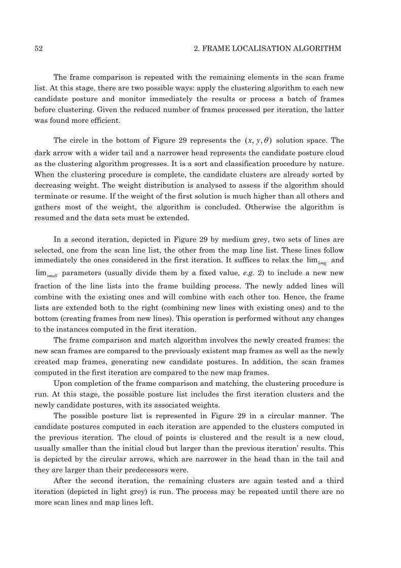
The frame comparison is repeated with the remaining elements in the scan frame list. At this stage, there are two possible ways: apply the clustering algorithm to each new candidate posture and monitor immediately the results or process a batch of frames before clustering. Given the reduced number of frames processed per iteration, the latter was found more efficient.
The circle in the bottom of Figure 29 represents the ),,( θyx solution space. The
dark arrow with a wider tail and a narrower head represents the candidate posture cloud as the clustering algorithm progresses. It is a sort and classification procedure by nature. When the clustering procedure is complete, the candidate clusters are already sorted by decreasing weight. The weight distribution is analysed to assess if the algorithm should terminate or resume. If the weight of the first solution is much higher than all others and gathers most of the weight, the algorithm is concluded. Otherwise the algorithm is resumed and the data sets must be extended.
In a second iteration, depicted in Figure 29 by medium grey, two sets of lines are
selected, one from the scan line list, the other from the map line list. These lines follow immediately the ones considered in the first iteration. It suffices to relax the longlim and
smalllim parameters (usually divide them by a fixed value, e.g. 2) to include a new new
fraction of the line lists into the frame building process. The newly added lines will combine with the existing ones and will combine with each other too. Hence, the frame lists are extended both to the right (combining new lines with existing ones) and to the bottom (creating frames from new lines). This operation is performed without any changes to the instances computed in the first iteration.
The frame comparison and match algorithm involves the newly created frames: the new scan frames are compared to the previously existent map frames as well as the newly created map frames, generating new candidate postures. In addition, the scan frames computed in the first iteration are compared to the new map frames.
Upon completion of the frame comparison and matching, the clustering procedure is run. At this stage, the possible posture list includes the first iteration clusters and the newly candidate postures, with its associated weights.
The possible posture list is represented in Figure 29 in a circular manner. The candidate postures computed in each iteration are appended to the clusters computed in the previous iteration. The cloud of points is clustered and the result is a new cloud, usually smaller than the initial cloud but larger than the previous iteration’ results. This is depicted by the circular arrows, which are narrower in the head than in the tail and they are larger than their predecessors were.
After the second iteration, the remaining clusters are again tested and a third iteration (depicted in light grey) is run. The process may be repeated until there are no more scan lines and map lines left.
2.5. IMPLEMENTATION ISSUES 53
In many trials, a single iteration of the algorithm is sufficient and two iterations cover most cases. The strategy used to constrain the calculations, associated to the relatively small number of instances turns the Frame Localisation algorithm into an efficient solution for the localisation problem, albeit its exponential nature.
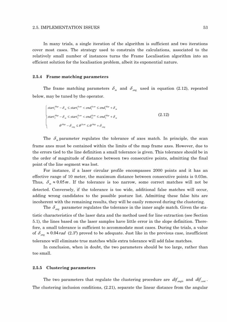
2.5.4 Frame matching parameters The frame matching parameters mδ and angδ used in equation (2.12), repeated
below, may be tuned by the operator. start start end end
start start end end
Mapm
Scan Scan Mapm
Mapm
Scan Scan Mapm
Mapang
Scan Mapang
1 1 1 1
2 2 21 2
− ≤ < ≤ +
− ≤ < ≤ +
− ≤ ≤ +
δ δ
δ δ
θ δ θ θ δ
(2.12)
The mδ parameter regulates the tolerance of axes match. In principle, the scan
frame axes must be contained within the limits of the map frame axes. However, due to the errors tied to the line definition a small tolerance is given. This tolerance should be in the order of magnitude of distance between two consecutive points, admitting the final point of the line segment was lost.
For instance, if a laser circular profile encompasses 2000 points and it has an effective range of 10 meter, the maximum distance between consecutive points is 0.03m. Thus, mm 05.0≈δ . If the tolerance is too narrow, some correct matches will not be
detected. Conversely, if the tolerance is too wide, additional false matches will occur, adding wrong candidates to the possible posture list. Admitting these false hits are incoherent with the remaining results, they will be easily removed during the clustering.
The angδ parameter regulates the tolerance in the inner angle match. Given the sta-
tistic characteristics of the laser data and the method used for line extraction (see Section 5.1), the lines based on the laser samples have little error in the slope definition. There-fore, a small tolerance is sufficient to accommodate most cases. During the trials, a value of radang 04.0≈δ (2.3º) proved to be adequate. Just like in the previous case, insufficient
tolerance will eliminate true matches while extra tolerance will add false matches. In conclusion, when in doubt, the two parameters should be too large, rather than
too small.
2.5.5 Clustering parameters The two parameters that regulate the clustering procedure are angledif and centdif .
The clustering inclusion conditions, (2.21), separate the linear distance from the angular

54 2. FRAME LOCALISATION ALGORITHM
distance. Thus, equations (2.21) verify if the candidate posture [ ]Tiiiii wyxp θ= is
within a cylindrical neighbourhood of cluster, [ ]Tclj
clj
clj
cljj wyxc θ= . This simple
solution hedges the problem of creating a common metrics with linear and angular distance, which is addressed in Appendix D.
The centdif parameter defines the maximum cluster radius and parameter angledif
defines half the “height” of the cylinder (see Figure 30). Given the posture distribution generated by Frame Localisation, the cloud of points is split into many sub-clouds where the distance between one point and the nearest cluster is usually much smaller than the distance between clusters. Since the Frame Localisation provides a typical accuracy of 0.05m and 0.02rad (1º), the two parameters may be tuned between these figures and their double.
x
y
θ
diffcent
diffangle
Figure 30 – The possible posture cloud in the solution space
In case a candidate posture lies outside these boundaries, then it should be
considered a different match position. However, should the Frame Localisation performance degrade under any particular conditions, the angledif and centdif parameters
should be updated accordingly.
2.6 Experimental Results
This section illustrates the sequence of steps of the Frame Localisation algorithm by means of a real trial conducted in an office-like environment. The room is approximately 8 meters long by 6 meters wide (see Figure 31). It has two walls covered with windows (left and bottom edges in Figure 31a) and the other two walls are white painted. This room and the results obtained there will be presented thoroughly in Chapter 3, Section 4.
The room model (Figure 31a) was computed offline, based on architectural plans of the floor. In addition to the walls and window frames, the room model includes three file cabinets (visible in Figure 31b, showing the north wall). The windows are made of two

2.6. EXPERIMENTAL RESULTS 55
plates of glass with a white buffer in between (visible in Figure 31c, depicting a fraction of the east wall). The reflectance coefficient is high, thus they act as partial mirrors.
north
wall
(a)
(b) (c)
Figure 31 – Map of a sample office room and two views: north wall and east wall These trials were performed with the AEST platform, equipped with the Acuity
laser with rotating mirror (see Chapter 1, Section 3). Two laser range profiles are presented in Figure 32. Each profile has approximately
2400 points distributed by π2 rad (360º). However, there is a blind angle behind the
sensor, corresponding to the volume of the robot, which is approximately 1.4 rad (80º) on the AEST. The sensor device is presented at the centre of the image. The two experiments were conducted with a few weeks interval, hence there are some differences in the line profiles.
The acquisition system is depicted in the centre of the image, with a longer axis pointing to the right, representing the front direction. The arc in front of the system at 1-meter distance represents the errors in the laser scan when aiming at the AEST (by convention, invalid measurements are assigned a –1.0 value). There are errors in other directions but they are occasional.
The orientation of the acquisition system relative to the windows is detected by the irregular pattern of range samples, opposite to the regular sequence of samples pointing
56 2. FRAME LOCALISATION ALGORITHM
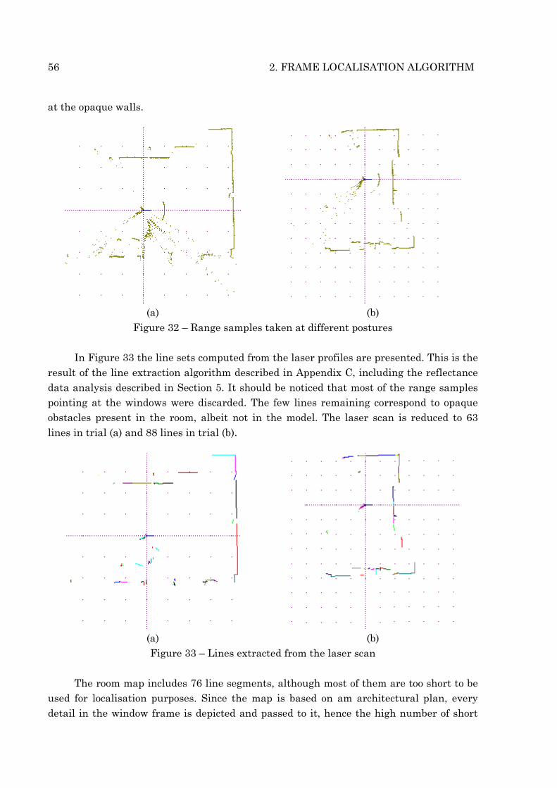
at the opaque walls.
(a) (b)
Figure 32 – Range samples taken at different postures In Figure 33 the line sets computed from the laser profiles are presented. This is the
result of the line extraction algorithm described in Appendix C, including the reflectance data analysis described in Section 5. It should be noticed that most of the range samples pointing at the windows were discarded. The few lines remaining correspond to opaque obstacles present in the room, albeit not in the model. The laser scan is reduced to 63 lines in trial (a) and 88 lines in trial (b).
(a) (b) Figure 33 – Lines extracted from the laser scan
The room map includes 76 line segments, although most of them are too short to be
used for localisation purposes. Since the map is based on am architectural plan, every detail in the window frame is depicted and passed to it, hence the high number of short

2.6. EXPERIMENTAL RESULTS 57
lines. The effective number of lines for localisation is close to 30. Based upon the line lists, the algorithm builds the frame lists. The scan frame list in
trial (a) includes 30 frames and 63 frames in trial (b). The main difference between the two trials is the lack of long lines in trial (b), leading to a higher number of scan frames. The map frame list has 17 elements in both cases.
The frame comparison and matching procedure generates the possible posture lists, illustrated in Figure 34.
Each candidate posture in Figure 34 is represented by a cross (the location of the scanning device and by a line segment representing the orientation. In trial (a) there are 42 candidate postures, whilst in trial (b) the number raises to 90. Many of these locations lie outside the depicted area. Since they result from matching with individual elements in the scene, there are no boundaries or contours to constrain the results.
From the analysis of Figure 34 some immediate conclusions may be drawn: • The square alignment of the surfaces organises the lines into two main
directions and the candidate postures follow two orthogonal orientations too. • The distance between clusters is much greater than the distance between the
elements of each cluster. • The environment symmetry, namely the periodic window distribution, induces
symmetric candidates in the solution space.
(a) (b)
Figure 34 – Possible posture lists Comparing the two trials, it is apparent that the reduced number of long lines,
which generated a larger number of frames is also at the origin of numerous frame matches and resulting posture candidates. It should be noticed that the candidate solutions are drawn without taking into to account their relative weight.
After the clustering procedure, illustrated in Figure 35, the neighbouring solutions are grouped and the isolated solutions are discarded. In trial (a) there are nine clusters in the figure and in trial (b) twenty-seven clusters are remaining. In Table 2, the proposed

58 2. FRAME LOCALISATION ALGORITHM
posture estimates are presented with their relative weight. Only the clusters with a relative weight greater than 0.04 are represented, the others are grouped.
The preferred solution is the one with the highest weight ( 0p ). Nevertheless, the
candidate solutions with weight greater than the threshold (0.04) are saved in the possible posture list for further analysis.
Trial (a) Trial (b)
x [m]
y [m]
θ
[rad]
w x [m]
y [m]
θ
[rad]
w
0p 4.137 2.481 -0.019 0.3936 3.593 3.000 1.541 0.2265
1p 4.156 2.909 -0.010 0.1405 3.575 3.425 1.537 0.1182
2p 3.718 1.154 1.551 0.1206 3.331 3.002 1.543 0.0807
3p 2.921 1.154 1.551 0.0978 4.771 7.257 -1.507 0.0705
4p 2.453 1.154 1.550 0.0931 3.352 10.153 -0.032 0.0439
5p 4.192 7.821 3.136 0.0779
6p 10.827 2.010 1.570 0.0479
plus 2 clusters with a total weight of 0.0268
plus 22 clusters with
a total weight of 0.4602
Table 2 – Results of Frame Localisation A simple comparison of weights within the same trial suggests the preferred
estimate be too close to the other estimates. In particular, in trial (b) the total weight of the neglected clusters is more than twice the weight of the preferred solution.
(a) (b)
Figure 35 – The possible posture list after clustering with the range data referred to the most likely solution
2.6. EXPERIMENTAL RESULTS 59
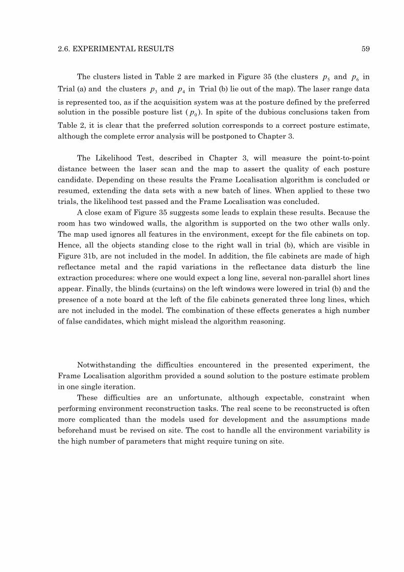
The clusters listed in Table 2 are marked in Figure 35 (the clusters 5p and 6p in
Trial (a) and the clusters 3p and 4p in Trial (b) lie out of the map). The laser range data
is represented too, as if the acquisition system was at the posture defined by the preferred solution in the possible posture list ( 0p ). In spite of the dubious conclusions taken from
Table 2, it is clear that the preferred solution corresponds to a correct posture estimate, although the complete error analysis will be postponed to Chapter 3.
The Likelihood Test, described in Chapter 3, will measure the point-to-point
distance between the laser scan and the map to assert the quality of each posture candidate. Depending on these results the Frame Localisation algorithm is concluded or resumed, extending the data sets with a new batch of lines. When applied to these two trials, the likelihood test passed and the Frame Localisation was concluded.
A close exam of Figure 35 suggests some leads to explain these results. Because the room has two windowed walls, the algorithm is supported on the two other walls only. The map used ignores all features in the environment, except for the file cabinets on top. Hence, all the objects standing close to the right wall in trial (b), which are visible in Figure 31b, are not included in the model. In addition, the file cabinets are made of high reflectance metal and the rapid variations in the reflectance data disturb the line extraction procedures: where one would expect a long line, several non-parallel short lines appear. Finally, the blinds (curtains) on the left windows were lowered in trial (b) and the presence of a note board at the left of the file cabinets generated three long lines, which are not included in the model. The combination of these effects generates a high number of false candidates, which might mislead the algorithm reasoning.
Notwithstanding the difficulties encountered in the presented experiment, the
Frame Localisation algorithm provided a sound solution to the posture estimate problem in one single iteration.
These difficulties are an unfortunate, although expectable, constraint when performing environment reconstruction tasks. The real scene to be reconstructed is often more complicated than the models used for development and the assumptions made beforehand must be revised on site. The cost to handle all the environment variability is the high number of parameters that might require tuning on site.