Print Page 1 2 3 4 5 6 7 8 9 10 11 12

Chapter 10: Testing Claims Regarding a Parameter10.1 The Language of Hypothesis Testing10.2 Hypothesis Tests for a Population Proportion10.3 Hypothesis Tests for a Population Mean10.4 Hypothesis Tests for a Population Standard Deviation10.5 Putting It Together: Which Method Do I Use?

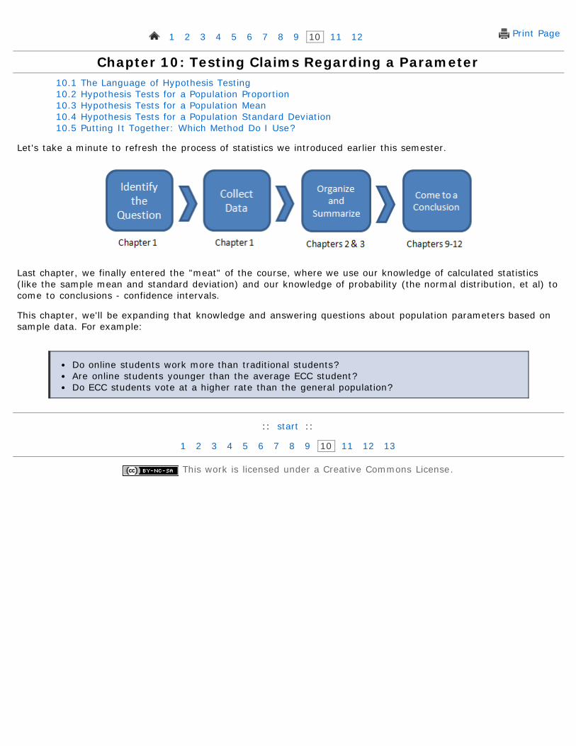
Let's take a minute to refresh the process of statistics we introduced earlier this semester.

Last chapter, we finally entered the "meat" of the course, where we use our knowledge of calculated statistics(like the sample mean and standard deviation) and our knowledge of probability (the normal distribution, et al) tocome to conclusions - confidence intervals.

This chapter, we'll be expanding that knowledge and answering questions about population parameters based onsample data. For example:

Do online students work more than traditional students?Are online students younger than the average ECC student?Do ECC students vote at a higher rate than the general population?

:: start ::

1 2 3 4 5 6 7 8 9 10 11 12 13

This work is licensed under a Creative Commons License.

Objectives

Print Page 1 2 3 4 5 6 7 8 9 10 11 12 13

Section 10.1: The Language of Hypothesis Testing10.1 The Language of Hypothesis Testing10.2 Hypothesis Tests for a Population Proportion10.3 Hypothesis Tests for a Population Mean10.4 Hypothesis Tests for a Population Standard Deviation10.5 Putting It Together: Which Method Do I Use?

By the end of this lesson, you will be able to...

1. determine the null and alternative hypotheses from a claim2. explain Type I and Type II errors3. identify whether an error is Type I or Type II4. state conclusions to hypothesis tests

The Nature of Hypothesis Testing

According to the US Census Bureau, 64% of US citizens age 18 or older voted in the 2004 election. Suppose webelieve that percentage is higher for ECC students for the 2008 presidential election. To determine if oursuspicions are correct, we collect information from a random sample of 500 ECC students. Of those, 460 werecitizens and 18 or older in time for the election. (We have some students still in high school, and some who donot yet have citizenship.) Of those who were eligible to vote, 326 (or about 71%) say that they did vote.

Problem: Based on this random sample, do we have enough evidence to say that the percentage of ECCstudents who were eligible to vote and did vote in the 2008 presidential election was higher than the proportionof US citizens who voted in the 2004 election?

Solution: 71% of the students in our sample voted. Obviously, this is higher than the national average. Thething to consider, though, is that this is just a sample of ECC students - it isn't every student. It's possible thatthe students who just happened to be in our sample were those who voted. Maybe this could just happenrandomly. In order to determine if it really is that different from the national proportion, we need to find out howprobable a sample proportion of 71% would be if the true proportion was really 64%.

To answer this, we consider the distribution of the proportion of eligible voters who did vote. From Section 8.2,we know that this proportion is approximately normally distributed if np(1-p)≥10. Using the techniques from thatsection, we also know that the mean would be 64%, with a standard deviation of about 2.2%. With thisinformation, the probability of observing a random sample with a proportion of 71% if the true proportion is 64%is about 0.001.

This means that about 1 in 1000 random samples will have a proportion that large. So we have two conclusions:

1. We just observed an extremely rare event, or2. The proportion of ECC students who vote is actually higher than 64%.

This is the idea behind hypothesis testing. The general process is this:

Steps in Hypothesis Testing

1. A claim is made. (More than 64% of ECC students vote, in our case.)2. Evidence is collected to test the claim. (We found that 326 of 460 voted.)3. The data are analyzed to assess the plausibility of the claim. (We determined that the proportion is

most likely higher than 64% for ECC students.)

Example 1

Example 2

Example 3

Null and Alternative Hypotheses

In statistics, we call these claims hypotheses. We have two types of hypotheses, a null hypothesis and analternative hypothesis.

The null hypothesis, denoted H0 ("H-naught"), is a statement to be tested. It is usually the status quo,and is assumed true until evidence is found otherwise.

The alternative hypothesis, denoted H1 ("H-one"), is a claim to be tested. We will try to find evidenceto support the alternative hypothesis.

There are three general ways in this chapter that we'll set up the null and alternative hypothesis.

1. two tailedH0: parameter = some valueH1: parameter ≠ the value

2. left-tailedH0: parameter = some valueH1: parameter < the value

3. right-tailedH0: parameter = some valueH1: parameter > the value

Let's look an example of each.

In the introduction of this section, we were considering the proportion ofECC students who voted in the 2008 presidential election. We assumedthat it was the same as the national proportion in 2004 (64%), and triedto find evidence that it was higher than that. In that case, our null andalternative hypotheses would be:

H0: p = 0.64H1: p > 0.64

According to the Elgin Community College website, the average age ofECC students is 28.2 years. We might claim that the average is less foronline Mth120 students. In that case, our null and alternative hypotheseswould be:

H0: μ = 28H1: μ < 28

It's fairly standard knowledge that IQ tests are designed to be normallydistributed, with an average of 100. We wonder whether the IQ of ECCstudents is different from this average. Our hypotheses would then be:

H0: μ = 100H1: μ ≠ 100

Example 4

The Four Outcomes of Hypothesis Testing

Unfortunately, we never know with 100% certainty what is true in reality. We always make our decision based onsample data, which may or may not reflect reality. So we'll make our decision, but it may not always be correct.

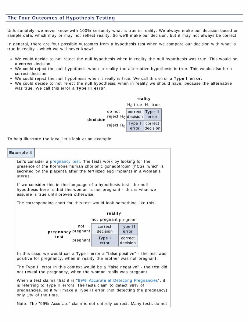
In general, there are four possible outcomes from a hypothesis test when we compare our decision with what istrue in reality - which we will never know!

We could decide to not reject the null hypothesis when in reality the null hypothesis was true. This would bea correct decision.We could reject the null hypothesis when in reality the alternative hypothesis is true. This would also be acorrect decision.We could reject the null hypothesis when it really is true. We call this error a Type I error.We could decide to not reject the null hypothesis, when in reality we should have, because the alternativewas true. We call this error a Type II error.

reality H0 true H1 true

decision

do notreject H0

correctdecision

Type IIerror

reject H0Type Ierror

correctdecision

To help illustrate the idea, let's look at an example.

Let's consider a pregnancy test. The tests work by looking for thepresence of the hormone human chorionic gonadotropin (hCG), which issecreted by the placenta after the fertilized egg implants in a woman'suterus.

If we consider this in the language of a hypothesis test, the nullhypothesis here is that the woman is not pregnant - this is what weassume is true until proven otherwise.

The corresponding chart for this test would look something like this:

reality not pregnant pregnant

pregnancytest

notpregnant

correctdecision

Type IIerror

pregnant Type Ierror

correctdecision

In this case, we would call a Type I error a "false positive" - the test waspositive for pregnancy, when in reality the mother was not pregnant.

The Type II error in this context would be a "false negative" - the test didnot reveal the pregnancy, when the woman really was pregnant.

When a test claims that it is "99% Accurate at Detecting Pregnancies", itis referring to Type II errors. The tests claim to detect 99% ofpregnancies, so it will make a Type II error (not detecting the pregnancy)only 1% of the time.

Note: The "99% Accurate" claim is not entirely correct. Many tests do not

Example 5

Example 6

have this accuracy until a few days after a missed period. (Source:USDept. of Health and Human Services)

Level of Significance

As notation, we assign two Greek letters, α ("alpha") and β ("beta"), to the probability of Type I and Type IIerrors, respectively.

α = P(Type I error) = P(rejecting H0 when H0 is true)

β = P(Type II error) = P(not rejecting H0 when H1 is true)

Unfortunately, we can't control both errors, so researchers choose the probability of making a Type I error beforethe sample is collected. We refer to this probability as the level of significance of the test.

Choosing α, the Probability of a Type I Error

One interesting topic is the choice of α. How do we choose? The answer to that is to consider the consequencesof the mistake. Consider two examples:

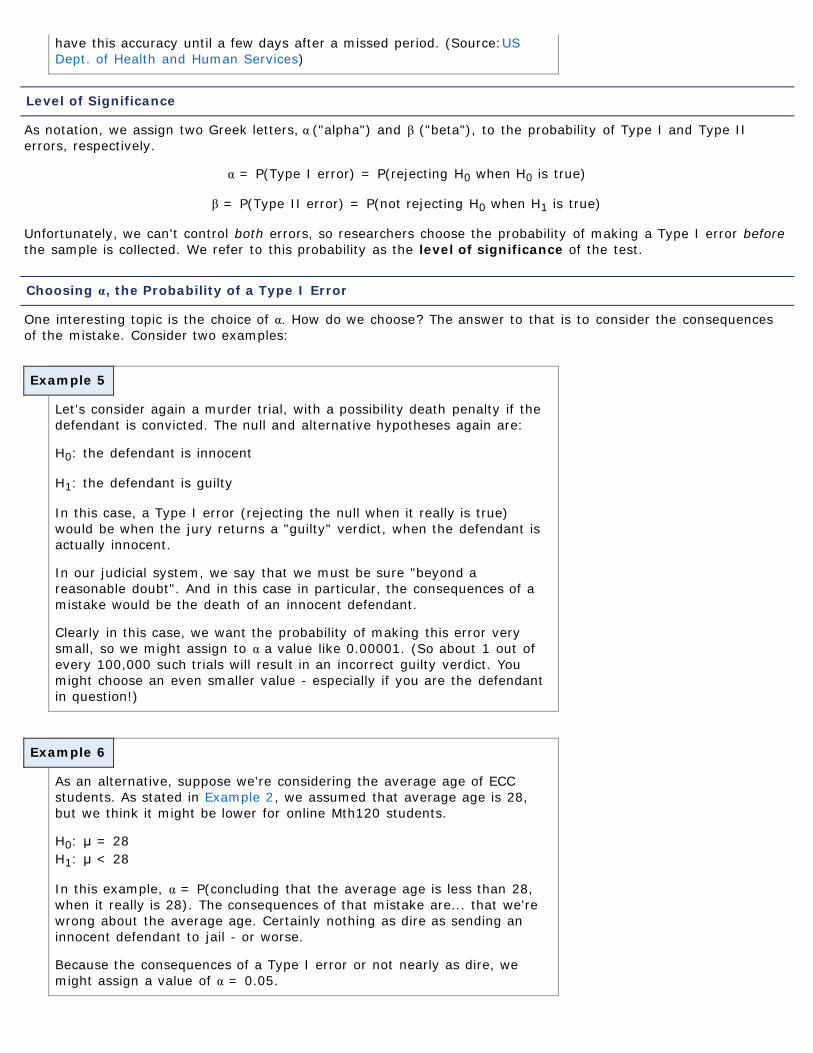
Let's consider again a murder trial, with a possibility death penalty if thedefendant is convicted. The null and alternative hypotheses again are:

H0: the defendant is innocent

H1: the defendant is guilty

In this case, a Type I error (rejecting the null when it really is true)would be when the jury returns a "guilty" verdict, when the defendant isactually innocent.

In our judicial system, we say that we must be sure "beyond areasonable doubt". And in this case in particular, the consequences of amistake would be the death of an innocent defendant.

Clearly in this case, we want the probability of making this error verysmall, so we might assign to α a value like 0.00001. (So about 1 out ofevery 100,000 such trials will result in an incorrect guilty verdict. Youmight choose an even smaller value - especially if you are the defendantin question!)

As an alternative, suppose we're considering the average age of ECCstudents. As stated in Example 2, we assumed that average age is 28,but we think it might be lower for online Mth120 students.

H0: μ = 28H1: μ < 28

In this example, α = P(concluding that the average age is less than 28,when it really is 28). The consequences of that mistake are... that we'rewrong about the average age. Certainly nothing as dire as sending aninnocent defendant to jail - or worse.

Because the consequences of a Type I error or not nearly as dire, wemight assign a value of α = 0.05.

Example 7

An Interesting Example of Type I and II Errors

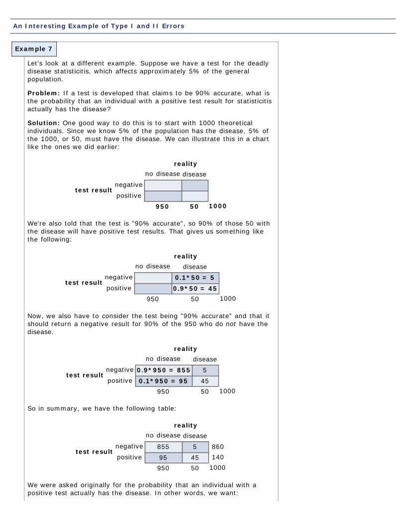
Let's look at a different example. Suppose we have a test for the deadlydisease statisticitis, which affects approximately 5% of the generalpopulation.

Problem: If a test is developed that claims to be 90% accurate, what isthe probability that an individual with a positive test result for statisticitisactually has the disease?

Solution: One good way to do this is to start with 1000 theoreticalindividuals. Since we know 5% of the population has the disease, 5% ofthe 1000, or 50, must have the disease. We can illustrate this in a chartlike the ones we did earlier:

reality no disease disease

test resultnegative positive

950 50 1000

We're also told that the test is "90% accurate", so 90% of those 50 withthe disease will have positive test results. That gives us something likethe following:

reality no disease disease

test resultnegative 0.1*50 = 5 positive 0.9*50 = 45

950 50 1000

Now, we also have to consider the test being "90% accurate" and that itshould return a negative result for 90% of the 950 who do not have thedisease.

reality no disease disease

test resultnegative 0.9*950 = 855 5 positive 0.1*950 = 95 45

950 50 1000

So in summary, we have the following table:

reality no disease disease

test resultnegative 855 5 860positive 95 45 140

950 50 1000

We were asked originally for the probability that an individual with apositive test actually has the disease. In other words, we want:

Example 8

Example 9

P(has disease | positive test) = 45/140 ≈ 0.32

What does this mean? Well, if this test is "90% accurate", then a positivetest result actually only means you have the disease about 32% of thetime!

On the other hand, it's interesting to note that a negative result is fairlyaccurate - 855/860 ≈ 0.994 = 99.4%. So you can feel pretty confident ofa negative result.

This may seem unreal, but some tests really do work this way. What is done to balance this out is to treat a"positive" test result as not definitive - it simply warrants more study.

The test for gestational diabetes is a perfect example. The test is performed in two stages - an initial "screening",which is extended to a second test if the result is positive.

Stating Conclusions to Hypothesis Tests

We have to be very careful when we state our conclusions. The way this type of hypothesis testing works, welook for evidence to support the alternative claim. If we find it, we say we have enough to support thealternative. If we don't find that evidence, we say just that - we don't have enough evidence to support thealternative hypothesis.

We never support the null hypothesis. In fact, the null hypothesis is probably not exactly true. There aresome very interesting discussions of this type of hypothesis testing (see links at the end of this page), and onecriticism is that large enough sample will probably show a difference from the null hypothesis.

That said, we look for evidence to support the alternative hypothesis. If we don't find it, then we simply say thatwe don't have enough evidence to support the alternative hypothesis.

To illustrate, consider the three examples from earlier this section:

Let's consider Example 1, introduced earlier this section. The null andalternative hypotheses were as follows:

H0: p = 0.64H1: p > 0.64

Suppose we decide that the evidence supports the alternative claim (itdoes). Our conclusion would then be:

There is enough evidence to support the claim that the proportion of ECCstudents who were eligible to vote and did was more than the nationalproportion of 64% who voted in 2004.

In Example 2, we stated null and alternative hypotheses:

H0: μ = 28H1: μ < 28

Suppose we find an average age of 20.4, and we decide to reject the nullhypothesis. Our conclusion would then be:

There is enough evidence to support our claim that the average age ofonline Mth120 students is less than 28 years.

Example 10

In Example 3, we stated null and alternative hypotheses:

H0: μ = 100H1: μ ≠ 100

Suppose we find an average IQ from a sample of 30 students to be 101,which we determine is not significantly different from the assumed mean.Our conclusion would then be:

There is not enough evidence to support the claim that the average IQ ofECC students is not 100.

The Controversy Regarding Hypothesis Testing

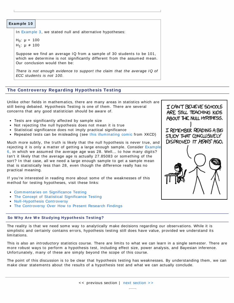
Unlike other fields in mathematics, there are many areas in statistics which arestill being debated. Hypothesis Testing is one of them. There are severalconcerns that any good statistician should be aware of.

Tests are significantly affected by sample sizeNot rejecting the null hypothesis does not mean it is trueStatistical significance does not imply practical significanceRepeated tests can be misleading (see this illuminating comic from XKCD)

Much more subtly, the truth is likely that the null hypothesis is never true, andrejecting it is only a matter of getting a large enough sample. Consider Example6, in which we assumed the average age was 28. Well... to how many digits?Isn't it likely that the average age is actually 27.85083 or something of thesort? In that case, all we need a large enough sample to get a sample meanthat is statistically less than 28, even though the difference really has nopractical meaning.

If you're interested in reading more about some of the weaknesses of thismethod for testing hypotheses, visit these links:

Commentaries on Significance TestingThe Concept of Statistical Significance TestingNull-Hypothesis ControversyThe Controversy Over How to Present Research Findings

So Why Are We Studying Hypothesis Testing?

The reality is that we need some way to analytically make decisions regarding our observations. While it issimplistic and certainly contains errors, hypothesis testing still does have value, provided we understand itslimitations.

This is also an introductory statistics course. There are limits to what we can learn in a single semester. There aremore robust ways to perform a hypothesis test, including effect size, power analysis, and Bayesian inference.Unfortunately, many of these are simply beyond the scope of this course.

The point of this discussion is to be clear that hypothesis testing has weaknesses. By understanding them, we canmake clear statements about the results of a hypothesis test and what we can actually conclude.

<< previous section | next section >>

1 2 3 4 5 6 7 8 9 10 11 12 13

This work is licensed under a Creative Commons License.

Objectives

Print Page 1 2 3 4 5 6 7 8 9 10 11 12 13

Section 10.2: Hypothesis Tests for a Population Proportion10.1 The Language of Hypothesis Testing10.2 Hypothesis Tests for a Population Proportion10.3 Hypothesis Tests for a Population Mean10.4 Hypothesis Tests for a Population Standard Deviation10.5 Putting It Together: Which Method Do I Use?

By the end of this lesson, you will be able to...

1. explain the logic of hypothesis testing2. test hypotheses about a population proportion3. test hypotheses about a population proportion using the binomial probability distribution

he Logic of Hypothesis Testing

Once we have our null and alternative hypotheses chosen, and our sample data collected, how do we choosewhether or not to reject the null hypothesis? In a nutshell, it's this:

If the observed results are unlikely assuming that the null hypothesis is true, we say the result isstatistically significant, and we reject the null hypothesis. In other words, the observed resultsare so unusual, that our original assumption in the null hypothesis must not have been correct.

Your textbook references three different methods for testing hypotheses:

the classical approachP-valuesconfidence intervals

Because P-values are so much more widely used, we will be focusing on this method. You will berequired to include P-values for your homework and exams.

If you're interested in learning any of these other methods, feel free to read through the textbook.

P-Values

In general, we define the P-value this way:

The P-value is the probability of observing a sample statistic as extreme or more extreme than the oneobserved in the sample assuming that the null hypothesis is true.

The Sample Proportion

In Section 8.2, we learned about the distribution of the sample proportion, so let's do a quick review of that now.

In general, if we let x = the number with the specific characteristic, then the sample proportion, ,(read "p-hat") is given by:

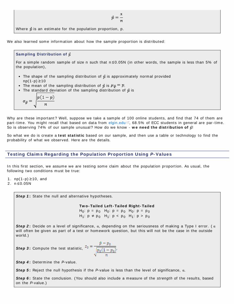
Where is an estimate for the population proportion, p.

We also learned some information about how the sample proportion is distributed:

Sampling Distribution of

For a simple random sample of size n such that n≤0.05N (in other words, the sample is less than 5% ofthe population),

The shape of the sampling distribution of is approximately normal provided np(1-p)≥10The mean of the sampling distribution of is .The standard deviation of the sampling distribution of is

Why are these important? Well, suppose we take a sample of 100 online students, and find that 74 of them arepart-time. You might recall that based on data from elgin.edu , 68.5% of ECC students in general are par-time.So is observing 74% of our sample unusual? How do we know - we need the distribution of !

So what we do is create a test statistic based on our sample, and then use a table or technology to find theprobability of what we observed. Here are the details.

Testing Claims Regarding the Population Proportion Using P-Values

In this first section, we assume we are testing some claim about the population proportion. As usual, thefollowing two conditions must be true:

1. np(1-p)≥10, and2. n≤0.05N

Step 1: State the null and alternative hypotheses.

Two-TailedH0: p = p0H1: p ≠ p0

Left-TailedH0: p = p0H1: p < p0

Right-TailedH0: p = p0H1: p > p0

Step 2: Decide on a level of significance, α, depending on the seriousness of making a Type I error. ( αwill often be given as part of a test or homework question, but this will not be the case in the outsideworld.)

Step 3: Compute the test statistic, .

Step 4: Determine the P-value.

Step 5: Reject the null hypothesis if the P-value is less than the level of significance, α.

Step 6: State the conclusion. (You should also include a measure of the strength of the results, basedon the P-value.)

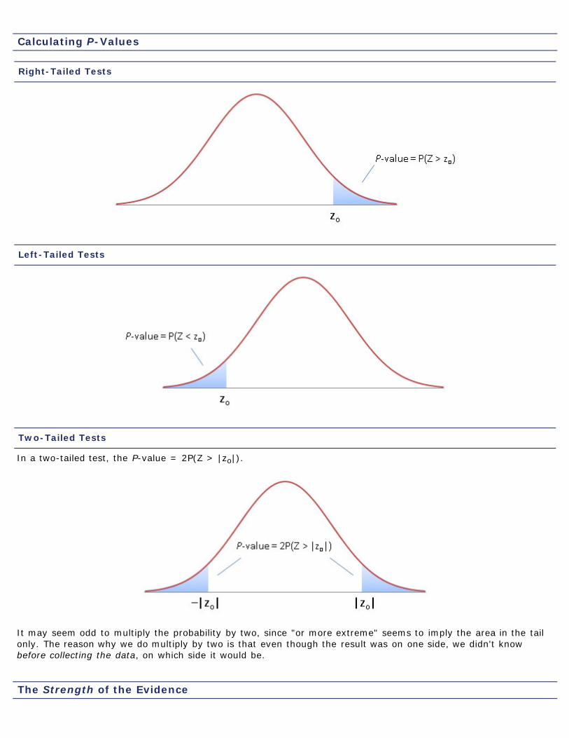
Calculating P-Values

Right-Tailed Tests

Left-Tailed Tests

Two-Tailed Tests

In a two-tailed test, the P-value = 2P(Z > |zo|).

It may seem odd to multiply the probability by two, since "or more extreme" seems to imply the area in the tailonly. The reason why we do multiply by two is that even though the result was on one side, we didn't knowbefore collecting the data, on which side it would be.

The Strength of the Evidence

Example 1

Example 2

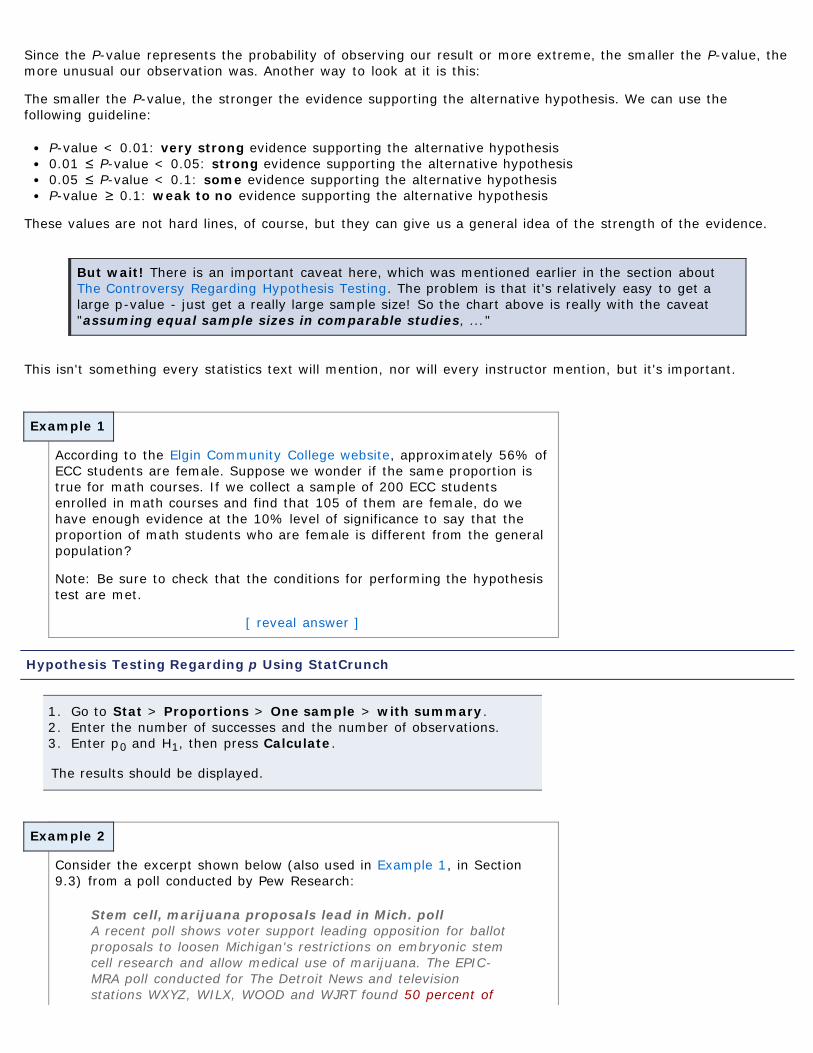
Since the P-value represents the probability of observing our result or more extreme, the smaller the P-value, themore unusual our observation was. Another way to look at it is this:

The smaller the P-value, the stronger the evidence supporting the alternative hypothesis. We can use thefollowing guideline:

P-value < 0.01: very strong evidence supporting the alternative hypothesis0.01 ≤ P-value < 0.05: strong evidence supporting the alternative hypothesis0.05 ≤ P-value < 0.1: some evidence supporting the alternative hypothesisP-value ≥ 0.1: weak to no evidence supporting the alternative hypothesis

These values are not hard lines, of course, but they can give us a general idea of the strength of the evidence.

But wait! There is an important caveat here, which was mentioned earlier in the section aboutThe Controversy Regarding Hypothesis Testing. The problem is that it's relatively easy to get alarge p-value - just get a really large sample size! So the chart above is really with the caveat"assuming equal sample sizes in comparable studies, ..."

This isn't something every statistics text will mention, nor will every instructor mention, but it's important.

According to the Elgin Community College website, approximately 56% ofECC students are female. Suppose we wonder if the same proportion istrue for math courses. If we collect a sample of 200 ECC studentsenrolled in math courses and find that 105 of them are female, do wehave enough evidence at the 10% level of significance to say that theproportion of math students who are female is different from the generalpopulation?

Note: Be sure to check that the conditions for performing the hypothesistest are met.

[ reveal answer ]

Hypothesis Testing Regarding p Using StatCrunch

1. Go to Stat > Proportions > One sample > with summary.2. Enter the number of successes and the number of observations.3. Enter p0 and H1, then press Calculate.

The results should be displayed.

Consider the excerpt shown below (also used in Example 1, in Section9.3) from a poll conducted by Pew Research:

Stem cell, marijuana proposals lead in Mich. pollA recent poll shows voter support leading opposition for ballotproposals to loosen Michigan's restrictions on embryonic stemcell research and allow medical use of marijuana. The EPIC-MRA poll conducted for The Detroit News and televisionstations WXYZ, WILX, WOOD and WJRT found 50 percent of

Example 3

likely Michigan voters support the stem cell proposal, 32percent against and 18 percent undecided. The telephone pollof 602 likely Michigan voters was conducted Sept. 22 throughWednesday. It has a margin of sampling error of plus or minus4 percentage points. (Source: Associated Press)

Suppose we wonder if the percent of Elgin Community College studentswho support stem cell research is different from this. If 61 of 100randomly selected ECC students support stem cell research, is thereenough evidence at the 5% level of signficance to support our claim?

Note: Be sure to check that the conditions for performing the hypothesistest are met.

[ reveal answer ]

One question you might have is, "What do we do if the conditions for the hypothesis test about p aren't met?"Great question!

In that case, we can no longer say that sample proportion, , is approximately normally distributed. What we doinstead is return to the binomial distribution, and just consider x, the number of successes. Let's do a quickreview of binomial probabilities.

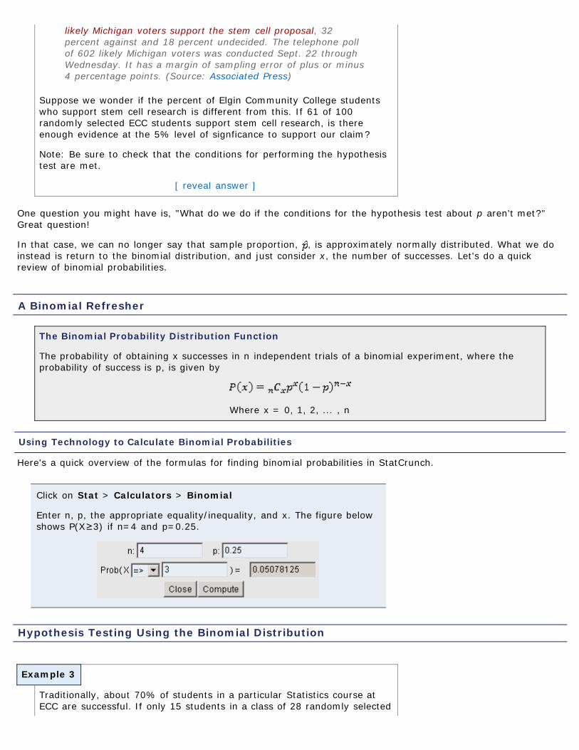
A Binomial Refresher

The Binomial Probability Distribution Function

The probability of obtaining x successes in n independent trials of a binomial experiment, where theprobability of success is p, is given by

Where x = 0, 1, 2, ... , n

Using Technology to Calculate Binomial Probabilities

Here's a quick overview of the formulas for finding binomial probabilities in StatCrunch.

Click on Stat > Calculators > Binomial

Enter n, p, the appropriate equality/inequality, and x. The figure belowshows P(X≥3) if n=4 and p=0.25.

Hypothesis Testing Using the Binomial Distribution

Traditionally, about 70% of students in a particular Statistics course atECC are successful. If only 15 students in a class of 28 randomly selected

students are successful, is there enough evidence at the 5% level ofsignificance to say that students of that particular instructor aresuccessful at a rate less than 70%?

[ reveal answer ]

<< previous section | next section >>

1 2 3 4 5 6 7 8 9 10 11 12 13

This work is licensed under a Creative Commons License.

Objectives

Print Page 1 2 3 4 5 6 7 8 9 10 11 12 13

Section 10.3: Hypothesis Tests for a Population Mean10.1 The Language of Hypothesis Testing10.2 Hypothesis Tests for a Population Proportion10.3 Hypothesis Tests for a Population Mean10.4 Hypothesis Tests for a Population Standard Deviation10.5 Putting It Together: Which Method Do I Use?

By the end of this lesson, you will be able to...

1. test hypotheses about a mean2. understand the difference between statistical significance and practical significance

In Section 10.2, we tested hypotheses regarding a population proportion. In this section, we'll consider claimsregarding μ, the population mean.

As we did in the previous section, we have some conditions that need to be true in order to perform the test(based on the Central Limit Theorem from Chapter 8).

1. the sample is obtained using simple random sampling, and2. the sample has no outliers and the population from which the sample is drawn is normally distributed, or the

sample size is large (n≥30)

The steps in performing the hypothesis test are nearly identical, with only a couple changes.

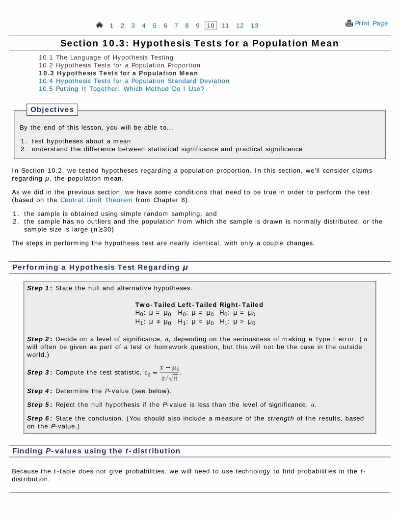
Performing a Hypothesis Test Regarding μ

Step 1: State the null and alternative hypotheses.

Two-TailedH0: μ = μ0H1: μ ≠ μ0

Left-TailedH0: μ = μ0H1: μ < μ0

Right-TailedH0: μ = μ0H1: μ > μ0

Step 2: Decide on a level of significance, α, depending on the seriousness of making a Type I error. ( αwill often be given as part of a test or homework question, but this will not be the case in the outsideworld.)

Step 3: Compute the test statistic, .

Step 4: Determine the P-value (see below).

Step 5: Reject the null hypothesis if the P-value is less than the level of significance, α.

Step 6: State the conclusion. (You should also include a measure of the strength of the results, basedon the P-value.)

Finding P-values using the t-distribution

Because the t-table does not give probabilities, we will need to use technology to find probabilities in the t-distribution.

Example 1

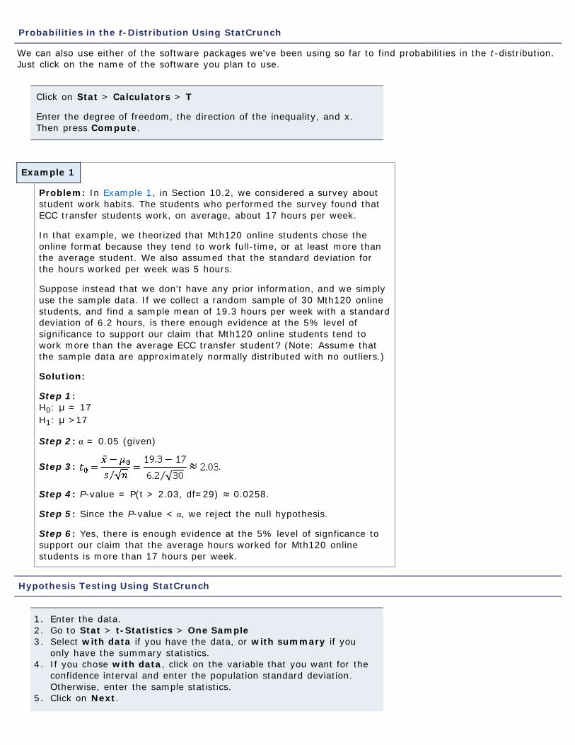
Probabilities in the t-Distribution Using StatCrunch

We can also use either of the software packages we've been using so far to find probabilities in the t-distribution.Just click on the name of the software you plan to use.

Click on Stat > Calculators > T

Enter the degree of freedom, the direction of the inequality, and x.Then press Compute.

Problem: In Example 1, in Section 10.2, we considered a survey aboutstudent work habits. The students who performed the survey found thatECC transfer students work, on average, about 17 hours per week.

In that example, we theorized that Mth120 online students chose theonline format because they tend to work full-time, or at least more thanthe average student. We also assumed that the standard deviation forthe hours worked per week was 5 hours.

Suppose instead that we don't have any prior information, and we simplyuse the sample data. If we collect a random sample of 30 Mth120 onlinestudents, and find a sample mean of 19.3 hours per week with a standarddeviation of 6.2 hours, is there enough evidence at the 5% level ofsignificance to support our claim that Mth120 online students tend towork more than the average ECC transfer student? (Note: Assume thatthe sample data are approximately normally distributed with no outliers.)

Solution:

Step 1:H0: μ = 17H1: μ >17

Step 2: α = 0.05 (given)

Step 3: .

Step 4: P-value = P(t > 2.03, df=29) ≈ 0.0258.

Step 5: Since the P-value < α, we reject the null hypothesis.

Step 6: Yes, there is enough evidence at the 5% level of signficance tosupport our claim that the average hours worked for Mth120 onlinestudents is more than 17 hours per week.

Hypothesis Testing Using StatCrunch

1. Enter the data.2. Go to Stat > t-Statistics > One Sample3. Select with data if you have the data, or with summary if you

only have the summary statistics.4. If you chose with data, click on the variable that you want for the

confidence interval and enter the population standard deviation.Otherwise, enter the sample statistics.

5. Click on Next.

Example 2

6. Enter μ0 and the alternative hypothesis.7. Click on Calculate.

The results should be displayed.

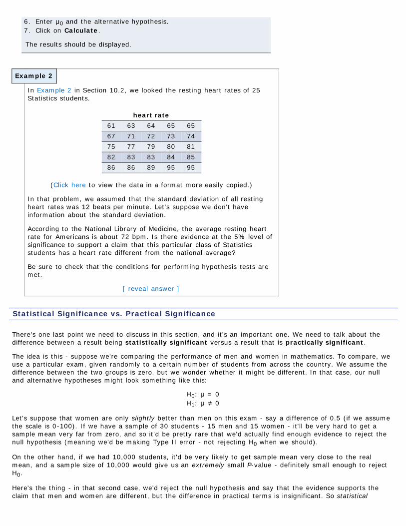
In Example 2 in Section 10.2, we looked the resting heart rates of 25Statistics students.

heart rate61 63 64 65 6567 71 72 73 7475 77 79 80 8182 83 83 84 8586 86 89 95 95

(Click here to view the data in a format more easily copied.)

In that problem, we assumed that the standard deviation of all restingheart rates was 12 beats per minute. Let's suppose we don't haveinformation about the standard deviation.

According to the National Library of Medicine, the average resting heartrate for Americans is about 72 bpm. Is there evidence at the 5% level ofsignificance to support a claim that this particular class of Statisticsstudents has a heart rate different from the national average?

Be sure to check that the conditions for performing hypothesis tests aremet.

[ reveal answer ]

Statistical Significance vs. Practical Significance

There's one last point we need to discuss in this section, and it's an important one. We need to talk about thedifference between a result being statistically significant versus a result that is practically significant.

The idea is this - suppose we're comparing the performance of men and women in mathematics. To compare, weuse a particular exam, given randomly to a certain number of students from across the country. We assume thedifference between the two groups is zero, but we wonder whether it might be different. In that case, our nulland alternative hypotheses might look something like this:

H0: μ = 0H1: μ ≠ 0

Let's suppose that women are only slightly better than men on this exam - say a difference of 0.5 (if we assumethe scale is 0-100). If we have a sample of 30 students - 15 men and 15 women - it'll be very hard to get asample mean very far from zero, and so it'd be pretty rare that we'd actually find enough evidence to reject thenull hypothesis (meaning we'd be making Type II error - not rejecting H0 when we should).

On the other hand, if we had 10,000 students, it'd be very likely to get sample mean very close to the realmean, and a sample size of 10,000 would give us an extremely small P-value - definitely small enough to rejectH0.

Here's the thing - in that second case, we'd reject the null hypothesis and say that the evidence supports theclaim that men and women are different, but the difference in practical terms is insignificant. So statistical

significance (enough evidence to reject the null hypothesis) doesn't necessarily imply practical significance.

Beware of studies with very large sample sizes that claim statistical significance. It may be thatthe differences have no practical meaning.

As an illustration, check out this comic from XKCD:

<< previous section | next section >>

1 2 3 4 5 6 7 8 9 10 11 12 13

This work is licensed under a Creative Commons License.

Objectives

Print Page 1 2 3 4 5 6 7 8 9 10 11 12 13

Section 10.4: Hypothesis Tests for a Population Standard Deviation10.1 The Language of Hypothesis Testing10.2 Hypothesis Tests for a Population Proportion10.3 Hypothesis Tests for a Population Mean10.4 Hypothesis Tests for a Population Standard Deviation10.5 Putting It Together: Which Method Do I Use?

By the end of this lesson, you will be able to...

1. test hypotheses about a population standard deviation

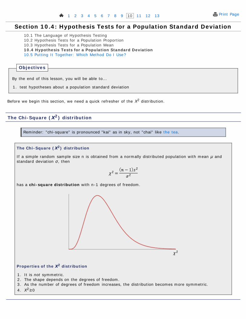
Before we begin this section, we need a quick refresher of the Χ2 distribution.

The Chi-Square (Χ2) distribution

Reminder: "chi-square" is pronounced "kai" as in sky, not "chai" like the tea.

The Chi-Square (Χ2) distribution

If a simple random sample size n is obtained from a normally distributed population with mean μ andstandard deviation σ, then

has a chi-square distribution with n-1 degrees of freedom.

Properties of the Χ2 distribution

1. It is not symmetric.2. The shape depends on the degrees of freedom.3. As the number of degrees of freedom increases, the distribution becomes more symmetric.4. Χ2≥0

Example 1

Finding Probabilities Using StatCrunch

Click on Stat > Calculators >Chi-Square

Enter the degrees of freedom, the direction of the inequality, and X.Then press Compute.

Performing a Hypothesis Test Regarding σ

Step 1: State the null and alternative hypotheses.

Two-TailedH0: σ = σ0H1: σ ≠ σ0

Left-TailedH0: σ = σ0H1: σ < σ0

Right-TailedH0: σ = σ0H1: σ > σ0

Step 2: Decide on a level of significance, α.

Step 3: Compute the test statistic, .

Step 4: Determine the P-value.

Step 5: Reject the null hypothesis if the P-value is less than the level of significance, α.

Step 6: State the conclusion.

In Example 2, in Section 10.2, we assumed that the standard deviationfor the resting heart rates of ECC students was 12 bpm. Later, inExample 2 in Section 10.3, we considered the actual sample data below.

heart rate61 63 64 65 6567 71 72 73 7475 77 79 80 8182 83 83 84 8586 86 89 95 95

(Click here to view the data in a format more easily copied.)

Based on this sample, is there enough evidence to say that the standarddeviation of the resting heart rates for students in this class is differentfrom 12 bpm?

Note: Be sure to check that the conditions for performing the hypothesistest are met.

[ reveal answer ]

Hypothesis Testing Regarding σ Using StatCrunch

Example 2

1. Go to Stat > Variance > One sample2. Select with data if you have the data, or with summary if you

only have the summary statistics.3. If you chose with data, click on the variable that you want for the

hypothesis test and press Next. Otherwise, enter the samplestatistics and press Next.

4. Enter the population variance (not standard deviation!) and the H15. Press Calculate.

The results should be displayed.

Let's look at Example 1 again, and try the hypothesis test withtechnology.

[ reveal answer ]

<< previous section | next section >>

1 2 3 4 5 6 7 8 9 10 11 12 13

This work is licensed under a Creative Commons License.

Objectives

Print Page 1 2 3 4 5 6 7 8 9 10 11 12 13

Section 10.5: Putting It Together: Which Method Do I Use?10.1 The Language of Hypothesis Testing10.2 Hypothesis Tests for a Population Proportion10.3 Hypothesis Tests for a Population Mean10.4 Hypothesis Tests for a Population Standard Deviation10.5 Putting It Together: Which Method Do I Use?

By the end of this lesson, you will be able to...

1. determine the appropriate hypothesis test to perform

Hypothesis Test Summary

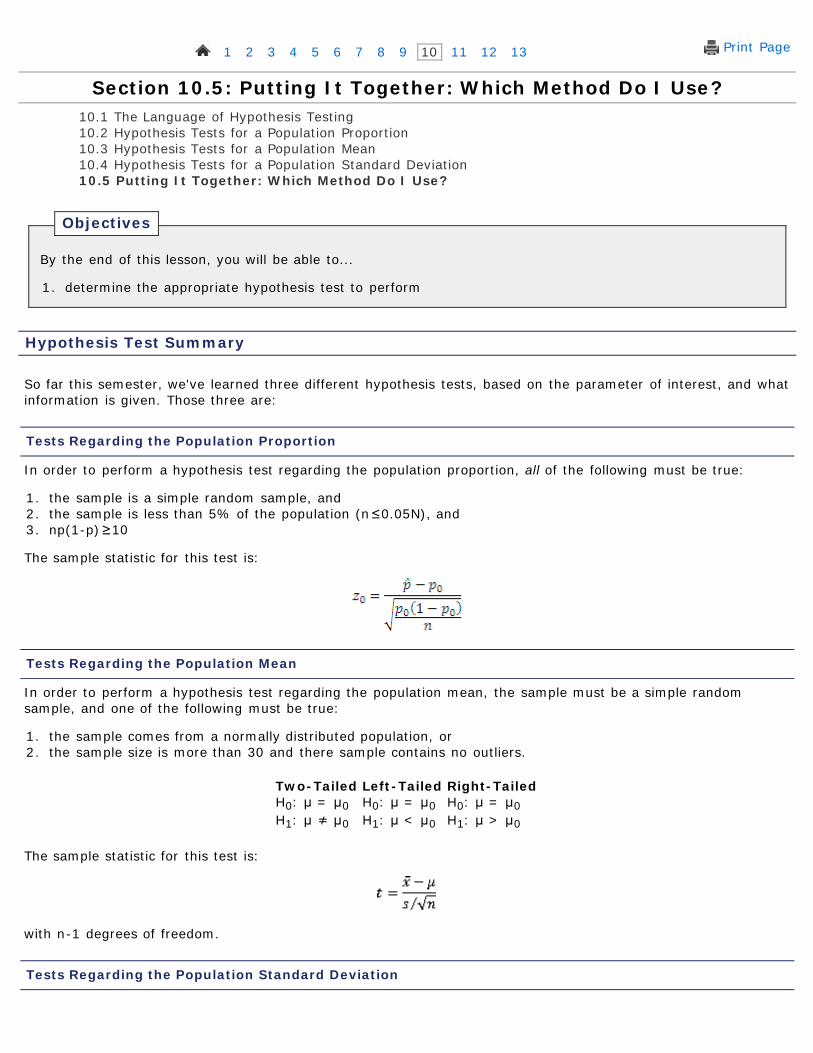
So far this semester, we've learned three different hypothesis tests, based on the parameter of interest, and whatinformation is given. Those three are:

Tests Regarding the Population Proportion

In order to perform a hypothesis test regarding the population proportion, all of the following must be true:

1. the sample is a simple random sample, and2. the sample is less than 5% of the population (n≤0.05N), and3. np(1-p)≥10

The sample statistic for this test is:

Tests Regarding the Population Mean

In order to perform a hypothesis test regarding the population mean, the sample must be a simple randomsample, and one of the following must be true:

1. the sample comes from a normally distributed population, or2. the sample size is more than 30 and there sample contains no outliers.

Two-TailedH0: μ = μ0H1: μ ≠ μ0

Left-TailedH0: μ = μ0H1: μ < μ0

Right-TailedH0: μ = μ0H1: μ > μ0

The sample statistic for this test is:

with n-1 degrees of freedom.

Tests Regarding the Population Standard Deviation

Example 1

Example 2

In order to perform a hypothesis test regarding the population standard deviation, the sample must come from anormally distributed population. In this case, the sample statistic is:

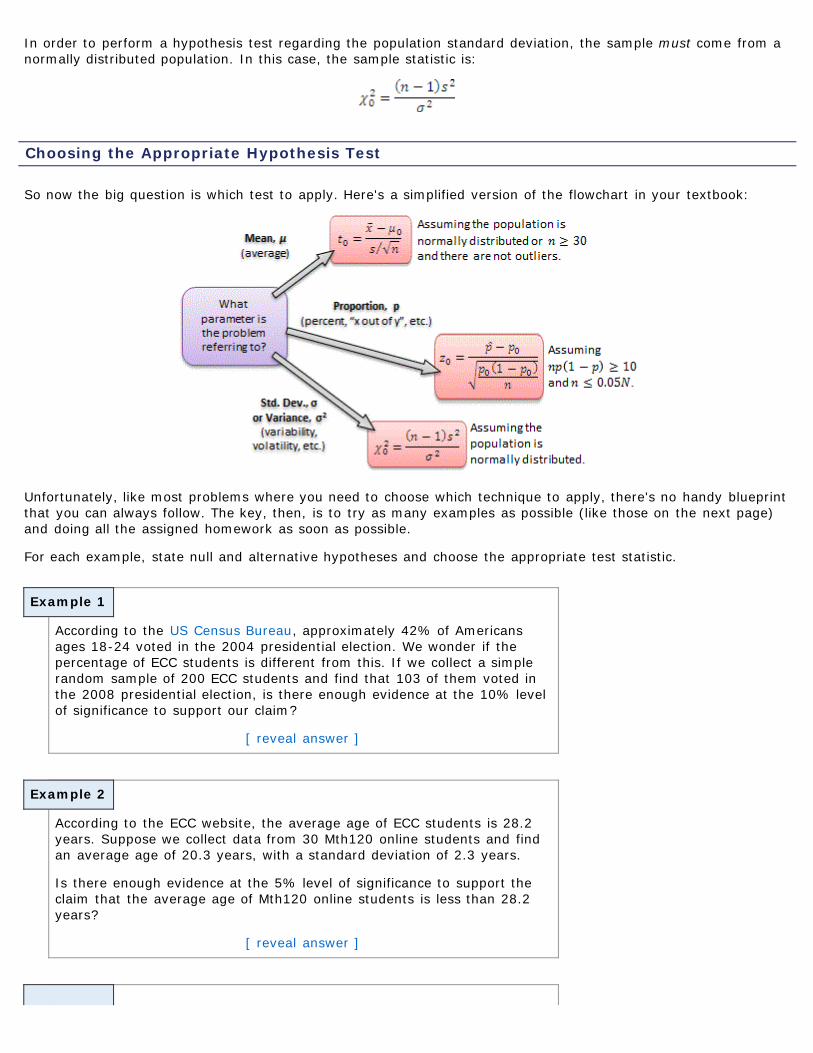
Choosing the Appropriate Hypothesis Test

So now the big question is which test to apply. Here's a simplified version of the flowchart in your textbook:

Unfortunately, like most problems where you need to choose which technique to apply, there's no handy blueprintthat you can always follow. The key, then, is to try as many examples as possible (like those on the next page)and doing all the assigned homework as soon as possible.

For each example, state null and alternative hypotheses and choose the appropriate test statistic.

According to the US Census Bureau, approximately 42% of Americansages 18-24 voted in the 2004 presidential election. We wonder if thepercentage of ECC students is different from this. If we collect a simplerandom sample of 200 ECC students and find that 103 of them voted inthe 2008 presidential election, is there enough evidence at the 10% levelof significance to support our claim?

[ reveal answer ]

According to the ECC website, the average age of ECC students is 28.2years. Suppose we collect data from 30 Mth120 online students and findan average age of 20.3 years, with a standard deviation of 2.3 years.

Is there enough evidence at the 5% level of significance to support theclaim that the average age of Mth120 online students is less than 28.2years?

[ reveal answer ]

Example 3

We know from previous examples that the standard deviation of IQs isnormally distributed with a standard deviation of 15. Suppose we wonderif the IQs of ECC students have more variation. To answer this question,we collect the IQs from a random sample of ECC students and find astandard deviation of 16.2.

Based on this information, is there enough evidence at the 5% level ofsignificance to say that the IQs of ECC students have more variation thanthe general population?

[ reveal answer ]

<< previous section | next section >>

1 2 3 4 5 6 7 8 9 10 11 12 13

This work is licensed under a Creative Commons License.