testing parallelism for the four-parameter logistic …

TESTING PARALLELISM FOR THE FOUR-PARAMETER LOGISTIC MODEL WITH D-

OPTIMAL DESIGN

A Thesis

Submitted to the Graduate Faculty

of the

North Dakota State University

of Agriculture and Applied Science

By

Ying Lin

In Partial Fulfillment of the Requirements.

for the Degree of

MASTER OF SCIENCE

Major Program:

Applied Statistics

February 2018

Fargo, North Dakota

North Dakota State University

Graduate School

Title

TESTING PARALLELISM FOR FOUR-PARAMETER LOGISTIC

MODEL WITH D-OPTIMAL DESIGN

By

Ying Lin

The Supervisory Committee certifies that this disquisition complies with North Dakota

State University’s regulations and meets the accepted standards for the degree of

MASTER OF SCIENCE

SUPERVISORY COMMITTEE:

Dr. Rhonda Magel

Chair

Dr. Seung Won Hyun

Dr. Yongki Choi

Approved:

May 21, 2018 Dr. Rhonda Magel

Date Department Chair

iii

ABSTRACT In order to determine the potency of the test preparation relative to the standard

preparation, it is often important to test parallelism between a pair of dose-response curves of

reference standard and test sample. Optimal designs are known to be more powerful in testing

parallelism as compared to classical designs. In this study, D-optimal design was implemented to

study the parallelism and compare its performance with a classical design. We modified D-

optimal design to test the parallelism in the four-parameter logistic (4PL) model using

Intersection-Union Test (IUT). IUT method is appropriate when the null hypothesis is expressed

as a union of sets, and by using this method complicated tests involving several parameters are

easily constructed. Since D-optimal design minimizes the variances of model parameters, it can

bring more power to the IUT test. A simulation study will be presented to compare the empirical

properties of the two different designs.

iv

ACKNOWLEDGEMENTS

I am grateful to all of the teachers and students in the Department of Statistics. They

have helped me develop solid an academic background.

I would like to thank Rhonda Magel and Yongki Choi who were willing to participate as

my defense committee. I would like to express my sincere gratitude and thanks to my advisor

Seung Won Hyun who has provided me professional guidance and taught me a great deal about

both scientific research and attitude towards work.

Finally, I would like to thank my parents and friends for encouraging me in all my

pursuits and inspiring me to follow my dreams.

v

TABLE OF CONTENTS

ABSTRACT ................................................................................................................................... iii

ACKNOWLEDGEMENTS ........................................................................................................... iv

LIST OF TABLES ......................................................................................................................... vi

LIST OF FIGURES ...................................................................................................................... vii

LIST OF ABBREVIATIONS ...................................................................................................... viii

1. INTRODUCTION ............................................................................................................ 1

2. BACKGROUND .............................................................................................................. 4

2.1. Mathematical function .................................................................................................. 4

2.2. D-optimal design for four-parameter logistic model .................................................... 5

2.3. Intersection-union test .................................................................................................. 7

2.4. Modified D-optimal design for the IUT test ................................................................. 7

3. TEST FOR PARALLELISM AND EFFICIENT DESIGN ............................................. 9

4. SIMULATION STUDY ................................................................................................. 19

5. SUMMARY ................................................................................................................... 25

REFERENCES ............................................................................................................................. 26

APPENDIX A. R CODES FOR T-VALUES OF CLASSICAL DESIGN .................................. 28

APPENDIX B. R CODES FOR T-VALUES OF D-OPTIMAL DESIGN .................................. 30

APPENDIX C. R CODES FOR POWER OF CLASSICAL DESIGN ........................................ 33

APPENDIX D. R CODES FOR POWER OF D-OPTIMAL DESIGN ....................................... 38

vi

LIST OF TABLES

Table Page

1. Classical design for parallel example ....................................................................................... 10

2. D-optimal design for parallel example ..................................................................................... 13

3. Classical design for non-parallelism example from Ding and Bailey (2003) ........................... 14

4. D-optimal design for non-parallel example .............................................................................. 16

5. T value results for the two examples ........................................................................................ 18

6. Modified D-optimal design for two lines in case 1 ................................................................... 20




10. Modified D-optimal design for two lines in case 5 ................................................................. 22

11. The power for D-optimal design and Classical design ........................................................... 24

vii

LIST OF FIGURES

Figure Page

1. The simulated data and fitted curves for ten-dose bioassay (parallel) ...................................... 11

2. The simulated data and fitted curves for toxicity(non-parallel) ................................................ 15

viii

LIST OF ABBREVIATIONS

IUT ................................................................................................................Intersection-union test

4PL ..............................................................................................................Four-parameter logistic

1

1. INTRODUCTION

It is often important for scientists to determine the parallelism between sets of dose-

response data, typically to compare potency of a test preparation relative to a standard

preparation. For example, decrease or increase in Biomarker concentration is only reliably in

case parallelism between endogenous Biomarker and concentration-response curve is

demonstrated. What’s more, parallel testing can increase throughput and reduce test execution.

The method of testing parallelism will influence the efficiency of the whole process, and

even the rate of success. Traditionally parallelism test methods are intended for testing equality

between pairs of parameters between the two dose-response curves. To test the equality, one way

is to compute the joint confidence region. But it’s complicated when a nonlinear curve model is

used. Therefore, approximations are made to simplify the task, such as using the intersection of

marginal confidence intervals as an approximate confidence region (Callahan and Sajjadi, 2003;

Lansky, 2003). However, this approximation causes the confidence interval to be much larger

than it should be, resulting in curves being labeled as parallel when they are not.

The typical procedure to test equality between pairs of parameters is often done by F-test

that compares the fit of the full (non-parallel) model for the two groups to a reduced (parallel)

model (Council of Europe, 2011, Finney, 1964). However, it has been criticized as over-sensitive

to small deviations from parallelism in highly precise assays (Callahan and Sajjadi, 2003, Hauck

et al., 2005, Gottschalk and Dunn, 2005a).

Another approach, referred to as equivalence tests, assumes lack of similarity, and seeks

evidence to prove similarity (see Callahan and Sajjadi 2003 and Hauck et al., 2005). Based on

the equivalence tests, Berger (1982), Casella and Berger (1990), and Berger and Hsu (1996) gave

a more complete discussion of Intersection–Union Test(IUT) theory. IUT for practical

2

parallelism is often used in bioequivalence testing, and can be easily implemented by using a

sequence of one sided approximate t-tests, which can be readily constructed using the output

from standard nonlinear regression software. It may provide more reliable and satisfying

inference than the other methods, in the sense that rejecting the null hypothesis establishes

evidence in favor of practically parallel response curves. So IUT is considered for testing

parallelism in this research.

One important factor for the success of testing parallelism is how to design the

experiment. An optimal design specifies how to distribute resources over doses in the most

efficient manner and the dose levels at which to take observations. Optimal designs, by

facilitating the data-collection process and subsequent data analysis in a cost-effective manner,

are more flexible and efficient, while classical designs require a greater number of experimental

runs to estimate interesting parameters with the same precision as an optimal design.

In practical terms, optimal designs can provide accurate statistical inference with

minimum cost. They minimize the variances of estimating interesting parameters and make

prediction without bias. Optimal designs use different criteria based on the goal of the

experiment. In general searching optimal designs for linear models with normal error is not so

complicate. The Fisher information matrix for a linear model is independent from the model

parameters, so the optimal designs are obtained in an explicit form. In practical situations,

however, many natural phenomena follow nonlinear models. Efficient designs for nonlinear

models are needed in a multitude of application areas. Under nonlinear models, the Fisher

information matrix depends on the unknown model parameters.

Searching optimal designs for nonlinear model is a complicated process, so scientists

usually relied on software to get more accurate outputs. As a software user, it is important to

3

select an efficient one from all types of algorithms so that the whole computing process can be

accelerated and the time for algorithm competition can be shortened. Furthermore, choosing a

proper algorithm can not only prevent the situation that there are special cases in which the

software won’t work quickly, but also avoid that it will produce unacceptable results.

Even though there are so many optimal design methods we can use to test parallelism, we

just studied D-optimal design in this paper. This type of optimal design is constructed to

minimize the generalized variance of the estimated regression coefficients. D-optimality is a

powerful experimental design for the determination of parallelism in biological applications,

because it minimizes the variance of estimating the model parameters and this helps to increase

the power of IUT test. D-optimal design for logistic models with four parameters was introduced

by Li and Majumdar (2007). Proper modification is made on the D-optimal design to use it for

the IUT test. In order to check the performance of the modified D-optimal design, we conduct

simulation studies to compare the power of IUT test under several scenarios with the design used

in the paper (Jonkman and Sidik, 2009).

Section 1 gives introduction about the definition of D-optimal and the motivation of

using it for testing parallelism. In Section 2, we suggest a simple method of testing the

hypothesis based on the IUT and explain the algorithm we used to search D-optimal design. Two

examples that illustrate the procedure of D-optimal design and contrast it with classical design

are considered in Section 3. A simulation study involving cases based on one of the examples is

presented and some of the implications of the simulation results are discussed in Section 4. A

brief discussion and summary is presented in Section 5.

4

2. BACKGROUND

Parallelism is observed where the dose-response curve of the test sample is a horizontal

shift of that of the reference standard on the logarithmic dose axis. Mathematically, two

functions are parallel if one function can be obtained from the other by a scaling of the dose axis.

2.1. Mathematical function

Consider the 4-parameter logistic(4PL) model

Y = 𝑎 +𝑑−𝑎

1+e[𝑏(𝑐−𝑋)] + 𝜀, 𝜀 𝑖𝑖𝑑~

𝑁(0, 𝜎2),

with unknown 𝜎2, which we have generally found useful in working with drug discovery

scientists. we typically work in the log base 10 scale for the dose level. Y is the response of

interest and X is the logarithm of dose of a given preparation. The model has 4 parameters, θ =

(𝑎, 𝑏, 𝑐, 𝑑), where 𝑎 is the lower asymptote of the curve, 𝑑 is the upper asymptote of the curve, 𝑏

represents the slope of the regression line, and finally𝑐 is the logarithm of the dose corresponding

to a mean response midway between the lower and upper plateaus. Let 𝑎1, 𝑏1, 𝑐1, 𝑑1 are the

model parameters for a test group and 𝑎2, 𝑏2, 𝑐2, 𝑑2 are the model parameters for a standard

group.

Consider a test group and a standard group, if 𝑎, 𝑏, 𝑑 are equivalent (i.e., 𝑎1 = 𝑎2, 𝑏1 =

𝑏2, 𝑑1 = 𝑑2), then the horizontal distance between the response curves on the 𝑙𝑜𝑔𝑋 scale is a

constant 𝑐1 − 𝑐2. Hence the relative potency of the test sample compared to the standard may be

estimated as 𝑒𝑐1−𝑐2. If the two response curves are not parallel, then the relative potency changes

depending on the level of response, since the distance between the two curves is not constant.

Thus, it is standard practice to statistically test the assumption of parallelism prior to estimating

the relative potency. In this paper, we are interested in accessing the equivalence involving three

pairs of parameters, and suggest a simple method of testing the hypothesis based on the

5

intersection-union principle (IUT) (see Berger, 1982; Berger and Hsu, 1996; Casella and Berger,

1990).

2.2. D-optimal design for four-parameter logistic model

In the experiments, the goal of optimal design is to make the variances of interesting

parameters and prediction as small as possible. To minimize the variances, the levels of doses

and the distribution of subjects over the doses must be decided, depending on how many subjects

are available and the range of dose levels.

ξ = (𝑥1, 𝑥2, … 𝑥𝑠

𝑝1, 𝑝2, … 𝑝𝑠,)

A design ξ contains dose levels 𝑥1, 𝑥2, … 𝑥𝑠 and corresponding weights 𝑝1, 𝑝2, … 𝑝𝑠, where

s ≥ 4, 𝑝𝑡 > 0 and∑ 𝑝𝑡 = 1𝑠𝑡=1 . When the total number of doses in the experiment is n, the

number of replication for dose 𝑥t is 𝑛𝑡, which is the nearest integer of 𝑝𝑡 ∗ 𝑛, 𝑡 = 1,2, … , 𝑠.

The Fisher information matrix for the 4PL model is

I(θ, ξ) = −𝐸 [𝜕2

𝜕θ ∂θT 𝑙𝑜𝑔𝐿(θ, ξ)],

where the function L(θ, ξ) is the likelihood function for the data. The information matrix defined

above is very important in the traditional optimality criteria. This matrix not only depends on the

design matrix ξ but also the unknown parameters θ. The design matrix ξ is usually chosen to

optimize certain function of the Fisher information matrix.

The D-optimality criterion is to choose a design maximizing the information on θ by

minimizing the generalized variance of its estimate. Denote θ̂ by the maximum likelihood

estimate of θ, then the asymptotic variance matrix of θ̂ is the inverse of the Fisher information

matrix I(θ, ξ). The commonly used D-optimality criterion, which minimizes the generalized

variance of θ̂, is equivalent to maximize the determinant of the Fisher information matrix, i.e.,

6

ξ∗ =𝑚𝑎𝑥ξ ∈ 𝐷 𝐷𝑒𝑡 [

𝐼(ξ, 𝜃)

𝑁]

where D is the set of all possible designs. Since 𝑁 is a constant, the D-optimality criterion is just

to maximize the determinant of the Fisher information matrix. Using such an idea, ξ∗ is the true

D-optimal design.

V-algorithm is a general well-known numerical algorithm to obtain locally optimal

designs and was developed in 1972 (V.V. Fedorov, 1972). The algorithm selects one dose that

maximizes the sensitive function which is derived from the directional derivative of the optimal

criterion at each iteration and stops once the design satisfies the Equivalence Theorem (J.M.

McGree, J.A. Eccleston, and S.B. Duffull, 2008 and F. Pukelsheim, 2006).

The problem for V-algorithm is that sometimes it takes very long time to converge to the

locally optimal designs. A state-of-the art algorithm (YBT algorithm) was proposed to find

locally optimal designs for a single objective and showed that it outperformed to other current

algorithms including V-algorithm. Starting from a randomly selected initial design, the YBT

algorithm selects the dose that maximizes the sensitivity function and adds to the previously

selected designs. At the same time, their optimal weights are obtained directly using the Newton-

Raphson method (K. Quinn, 20016). However, the problem in YBT is that if the selected initial

design points far from the optimal design points, then the YBT requires a lot more time to

converge to an optimal design and sometimes it failed to do so. In this paper, the modified YBT

algorithm was employed to obtain the D-optimal designs (See Hyun, Wong and Yang, 2018).

The procedure was modified by selecting better starting design points via the V-algorithm, and

this improved the search speed to obtain the optimal designs (S.W. Hyun, and W.K. Wong.

Yang, 2013). The modified algorithm performs greatly to obtain all the optimal designs in this

paper.

7

2.3. Intersection-union test

In the context of the four-parameter logistic curve, establishing practical equivalence

enables the assessment of relative potency via the parameters 𝑐1 and 𝑐2. We test whether the

lower and upper plateaus a and d, and the slope factor b, are equivalent for the test and control

group. Thus, stating the hypotheses in terms of unions and intersections, we are interested in

testing

𝐻0:

𝑎1 − 𝐷𝐿𝑎2 ≤ 0 𝑜𝑟 𝑎1 − 𝐷𝑈𝑎2 ≥ 0 𝑜𝑟 𝑏1 − 𝐷𝐿𝑏2 ≤ 0 𝑜𝑟 𝑏1 − 𝐷𝑈𝑏2 ≥ 0 𝑜𝑟

𝑑1 − 𝐷𝐿𝑑2 ≤ 0 𝑜𝑟 𝑑1 − 𝐷𝑈𝑑2 ≥ 0

versus

𝐻1:

𝑎1 − 𝐷𝐿𝑎2 > 0 𝑎𝑛𝑑 𝑎1 − 𝐷𝑈𝑎2 < 0 𝑎𝑛𝑑 𝑏1 − 𝐷𝐿𝑏2 > 0 𝑎𝑛𝑑 𝑏1 − 𝐷𝑈𝑏2 < 0 𝑎𝑛𝑑

𝑑1 − 𝐷𝐿𝑑2 > 0 𝑎𝑛𝑑 𝑑1 − 𝐷𝑈𝑑2 < 0

where 𝐷𝐿 represent lower limits and 𝐷𝑈 represents upper limits.

According to the discussion of IUT theory (Berger (1982), Casella and Berger (1990),

and Berger and Hsu (1996)), this method is useful when the null hypothesis is expressed as a

union, and the alternative hypothesis is expressed as an intersection. The null hypothesis is true if

any of component parts are true since it is a union, and if any component of the intersection in

the alternative is false, the hypothesis is false. Thus, by constructing the test so that each

component of 𝐻0 is tested separately at level α, and 𝐻0 is rejected only if all the component tests

reject, the IUT will have at most level α without requiring any multiplicity adjustment.

2.4. Modified D-optimal design for the IUT test

ξ𝐷(𝑇) and ξ𝐷(𝐶) works best for estimating model parameters for test and control lines

respectively, so combing both designs and using them for testing parallelism could be useful.

ξ𝐷(𝑇) = (𝑥T1, 𝑥T2, … 𝑥𝑇𝑠

𝑝T1, 𝑝T2, … 𝑝𝑇𝑠)

8

ξ𝐷(𝐶) = (𝑥C1, 𝑥C2, … 𝑥𝐶𝑠

𝑝C1, 𝑝C2, … 𝑝𝐶𝑠)

Propose ξ𝐷(𝐼𝑈𝑇) = α ∗ ξ𝐷(𝑇) + (1 − 𝛼) ∗ ξ𝐷(𝐶), where α is relative importance of

ξ𝐷(𝑇) 𝑡𝑜 ξ𝐷(𝐶). Under the assumption both designs are equally important, set α = 0.5. The

modified D-optimal design ξ𝐷(𝐼𝑈𝑇) is obtained by

ξ𝐷(𝐼𝑈𝑇) = (𝑥T1, 𝑥T2, … , 𝑥𝑇𝑠, 𝑥C1, 𝑥C2, … , 𝑥𝐶𝑠

α𝑝T1, α𝑝T2, … , α𝑝𝑇𝑠, (1 − 𝛼)𝑝T1, (1 − 𝛼)𝑝T2, … , (1 − 𝛼)𝑝𝑇𝑠),

If some design points between ξ𝐷(𝑇) and ξ𝐷(𝐶) are overlapped, put only one design point with

their weight sum (i.e., if 𝑥Ti = 𝑥Cj, them use only 𝑥Ti with corresponding weight α𝑝𝑇𝑖 + (1 −

α)𝑝𝐶𝑗.).

9

3. TEST FOR PARALLELISM AND EFFICIENT DESIGN

We statistically test the assumption of parallelism prior to estimating the relative potency,

since the potency of the test sample compared to the standard is defined simply in terms of the

parameter 𝑐𝑖 if the response curves for the two preparations are parallel.

𝐻0:

𝑎1 − 𝐷𝐿𝑎2 ≤ 0 𝑜𝑟 𝑎1 − 𝐷𝑈𝑎2 ≥ 0 𝑜𝑟 𝑏1 − 𝐷𝐿𝑏2 ≤ 0 𝑜𝑟 𝑏1 − 𝐷𝑈𝑏2 ≥ 0 𝑜𝑟

𝑑1 − 𝐷𝐿𝑑2 ≤ 0 𝑜𝑟 𝑑1 − 𝐷𝑈𝑑2 ≥ 0

versus

𝐻1:

𝑎1 − 𝐷𝐿𝑎2 > 0 𝑎𝑛𝑑 𝑎1 − 𝐷𝑈𝑎2 < 0 𝑎𝑛𝑑 𝑏1 − 𝐷𝐿𝑏2 > 0 𝑎𝑛𝑑 𝑏1 − 𝐷𝑈𝑏2 < 0 𝑎𝑛𝑑

𝑑1 − 𝐷𝐿𝑑2 > 0 𝑎𝑛𝑑 𝑑1 − 𝐷𝑈𝑑2 < 0,

𝐷𝐿, 𝐷𝑈 are the equivalence limits, and the choice of the two numbers should be carefully

considered, based on historical data and information from scientists at the assay laboratory, etc.

For example, the FDA Division of Bioequivalence (FDA 1992) uses 𝐷𝐿 = 0.8 and 𝐷𝑈 = 1.25

for bioequivalence hypotheses about ratios.

For 𝐻01: 𝑎1 − 𝐷𝐿𝑎2 ≤ 0 versus 𝐻11: 𝑎1 − 𝐷𝐿𝑎2 > 0, using a statistic of the form

𝑇1 =�̂�1 − 𝐷𝐿�̂�2

𝑠. 𝑒. (�̂�1 − 𝐷𝐿�̂�2)

s. e(�̂�1 − 𝐷𝐿�̂�2) = sqrt(var(�̂�1) + 𝐷𝐿2var(�̂�2))

Reject 𝐻01: 𝑎1 − 𝐷𝐿𝑎2 ≤ 0 if 𝑇1 > 𝑡𝑁−8,∝, where N is total sample size, and α is type I

error rate or significance level. Similarly, for 𝐻02: 𝑎1 − 𝐷𝑈𝑎2 ≥ 0 versus 𝐻12: 𝑎1 − 𝐷𝑈𝑎2 < 0,

using 𝑇2 =�̂�1−𝐷𝑈�̂�2

𝑠.𝑒.(�̂�1−𝐷𝑈�̂�2), Reject 𝐻02 if 𝑇2 < −𝑡𝑁−8,∝.

The remaining four tests proceed in analogous fashion. Reject 𝐻0 only if all six one side

approximate t-test reject 𝐻01, , , , , , 𝐻06 at the same α level (Berger, 1982; Berger and Hsu, 1996;

Casella and Berger, 1990).

10

Examples given by Dykstra (1971) to illustrate the difference between classical design

with D-optimal design. One experiment is ten-dose bioassay whose dose-response curves are

parallelism, with 3 reps, 10 doses and 𝑙𝑜𝑔10(𝑑𝑜𝑠𝑒) ⊂ [1.1, 3.8], and it has a response 𝑌1jk, 𝑗 =

1,2, … ,10, k = 1,2,3. Another experiment is toxicity assay whose dose-response curves are non-

parallelism, with 4 reps, 12 doses, and 𝑙𝑜𝑔10(𝑑𝑜𝑠𝑒) ⊂ [3.5, 9], and it has a response 𝑌2jk, 𝑗 =

1,2, … ,12, k = 1,2,3,4.

In the ten-dose bioassay, the parameters from Jonkman and Sidik (2009) are

𝜎12 = 𝜎2

2 = 0.042, 𝜖1~𝑁(0, 0.042), 𝜖2~𝑁(0, 0.042)

𝑎1 = 2.02, 𝑏1 = −1.42, 𝑐1 = 2.31, 𝑑1 = 10.12;

𝑎2 = 2.04, 𝑏2 = −1.35, 𝑐2 = 2.59, 𝑑2 = 9.86.

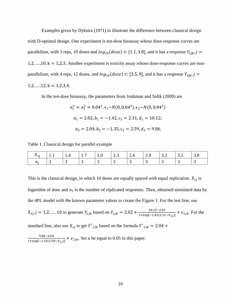
Table 1. Classical design for parallel example

𝑋1j 1.1 1.4 1.7 2.0 2.3 2.6 2.9 3.2 3.5 3.8

𝑛𝑡 3 3 3 3 3 3 3 3 3 3

This is the classical design, in which 10 doses are equally spaced with equal replication. 𝑋1j is

logarithm of dose and 𝑛𝑡 is the number of replicated responses. Then, obtained simulated data by

the 4PL model with the known parameter values to create the Figure 1. For the test line, use

𝑋1j, 𝑗 = 1,2, … , 10 to generate 𝑌1𝑗𝑘 based on 𝑌1𝑗𝑘 = 2.02 +10.12−2.02

1+exp [−1.42(2.31−𝑋1j)]+ 𝜖1𝑗𝑘. For the

standard line, also use 𝑋1j to get 𝑌′1𝑗𝑘 based on the formula 𝑌′

1𝑗𝑘 = 2.04 +

9.86−2.04

1+exp [−1.35(2.59−𝑋1𝑗)]+ 𝜖2𝑗𝑘. Set α be equal to 0.05 in this paper.

11

Figure 1. The simulated data and fitted curves for ten-dose bioassay (parallel)

Used the nonlinear least-squares estimates method to get the estimated parameters based

on the simulated data. In least square regression, a regression model was established, in which

the sum of the squares of the vertical distances of different points from the regression curve is

minimized. Estimated parameters are as follows:

�̂�1 = 2.08, �̂�1 = −1.45, �̂�1 = 10.04, �̂�2 = 2.06, �̂�2 = −1.34, �̂�2 = 10.15

𝑣𝑎𝑟(�̂�1) = 0.092, 𝑣𝑎𝑟(�̂�1) = 0.052, 𝑣𝑎𝑟(�̂�1) = 0.112

𝑣𝑎𝑟(�̂�2) = 0.112, 𝑣𝑎𝑟(�̂�2) = 0.042, 𝑣𝑎𝑟(�̂�2) = 0.092

Test the parallelism using this simulated data. For parameter 𝑎, make an inference as

follow: 𝐻01: 𝑎1 − 𝐷𝐿𝑎2 ≤ 0 versus 𝐻11: 𝑎1 − 𝐷𝐿𝑎2 > 0. 𝑇1 =�̂�1−𝐷𝐿�̂�2

𝑠.𝑒.(�̂�1−𝐷𝐿�̂�2)= 3.58, reject 𝐻01

since 𝑇1 > 𝑡58,0.05 = 1.67. 𝐻02: 𝑎1 − 𝐷𝑈𝑎2 ≥ 0 versus 𝐻12: 𝑎1 − 𝐷𝑈𝑎2 < 0.𝑇2 =�̂�1−𝐷𝑈�̂�2

𝑠.𝑒.(�̂�1−𝐷𝑈�̂�2)=

12

−2.94, reject 𝐻02 since 𝑇2 < −𝑡58,0.05 = −1.67. For parameter b, make an inference as follow:

𝐻01: 𝑏1 − 𝐷𝐿𝑏2 ≤ 0 versus 𝐻11: 𝑏1 − 𝐷𝐿𝑏2 > 0. Reject 𝐻01 since 𝑇1 = 6.32 > 𝑡58,0.05.𝐻02: 𝑏1 −

𝐷𝑈𝑏2 ≥ 0 versus 𝐻12: 𝑏1 − 𝐷𝑈𝑏2 < 0. Reject 𝐻02 since 𝑇2 = −3.10 < −𝑡58,0.05. For parameter

d, make an inference as follow: 𝐻01: 𝑑1 − 𝐷𝐿𝑑2 ≤ 0 versus 𝐻11: 𝑑1 − 𝐷𝐿𝑑2 > 0. Reject 𝐻01

since 𝑇1 = 14.34 > 𝑡58,0.05. 𝐻02: 𝑑1 − 𝐷𝑈𝑑2 ≥ 0 versus 𝐻12: 𝑑1 − 𝐷𝑈𝑑2 < 0. Reject 𝐻02 since

𝑇2 = −16.77 < −𝑡58,0.05. Since all six one side approximate t-test reject 𝐻01, 𝐻02, … , 𝐻06 at the

0.05 level, the dose-response curves are parallel since all the null hypothesis components are

rejected.

Then D-optimal design was motivated for testing parallelism. In Table 2, the first two

lines show the D-optimal design for the test line, the second two line show the D-optimal design

for the control line, and the last two lines show the modified D-optimal design for testing the

parallelism that can be used for fitting both test and control lines. In each design, the first row, X

represents the dose level in a logarithmic scale and the second row, P represents the proportion

of subjects at each selected dose level. The proportions of the modified D-optimal design were

obtained based on the formula 𝑃𝑀 = 0.5 ∗ 𝑃𝑇 + (1 − 0.5) ∗ 𝑃𝐶, where 𝑃𝑇 and 𝑃𝐶 are the proportions

of subjects in the two different lines, and the number of replicated responses of modified D-

optimal design is 𝑛𝑀, which is the nearest integer of 𝑃𝑀 ∗ 30 , where 30 is the number of subjects

that are used in test line and control line, respectively. For example, the modified D-optimal

design assigns seven replications at the first dose level of 1, one replication at the second dose

level of 1.88, and three replications at the third dose level 1.89, and so on.

13

Table 2. D-optimal design for parallel example

X Test line

1 1.88 1.89 2.95 4

𝑃𝑇 0.25 0.08 0.17 0.25 0.25

X Control line

1 1.99 3.08 4

𝑃𝐶 0.25 0.25 0.25 0.25

X

Modified D-optimal

1 1.88 1.89 1.99 2.95 3.08 4

𝑃𝑀 0.25 0.04 0.085 0.125 0.125 0.125 0.25

𝑛𝑀 7 1 3 4 4 3 8

For the test line, use the modified D-optimal design ξ = (X, 𝑛𝑡) to generate the response

𝑌1𝑗𝑘 based on 𝑌1𝑗𝑘 = 2.02 +10.12−2.02

1+exp [−1.42(2.31−𝑋)]+ 𝜖1𝑗𝑘. For the control line, also use ξ = (X, 𝑛𝑡)

to get 𝑌′1𝑗𝑘 based on the formula 𝑌′

1𝑗𝑘 = 2.04 +9.86−2.04

1+exp [−1.35(2.59−𝑋)]+ 𝜖2𝑗𝑘. we also used

nonlinear least-squares to obtain estimated parameters, which are as follows:

�̂�1 = 1.98, �̂�1 = −1.41, �̂�1 = 10.21, �̂�2 = 2.06, �̂�2 = −1.36, �̂�2 = 9.82

𝑣𝑎𝑟(�̂�1) = 0.032, 𝑣𝑎𝑟(�̂�1) = 0.032, 𝑣𝑎𝑟(�̂�1) = 0.052

𝑣𝑎𝑟(�̂�2) = 0.092, 𝑣𝑎𝑟(�̂�2) = 0.042, 𝑣𝑎𝑟(�̂�2) = 0.082

Test the parallelism using this simulated data. For parameter α, make an inference as

follow: 𝐻01: 𝑎1 − 𝐷𝐿𝑎2 ≤ 0 versus 𝐻11: 𝑎1 − 𝐷𝐿𝑎2 > 0. 𝑇1 =�̂�1−𝐷𝐿�̂�2

𝑠.𝑒.(�̂�1−𝐷𝐿�̂�2)= 4.11, reject 𝐻01

since 𝑇1 > 𝑡58,0.05 = 1.67. 𝐻02: 𝑎1 − 𝐷𝑈𝑎2 ≥ 0 versus 𝐻12: 𝑎1 − 𝐷𝑈𝑎2 < 0.𝑇2 =�̂�1−𝐷𝑈�̂�2

𝑠.𝑒.(�̂�1−𝐷𝑈�̂�2)=

−5.02, reject 𝐻02 since 𝑇2 < −𝑡58,0.05 = −1.67. For parameter b, make an inference as follow:

𝐻01: 𝑏1 − 𝐷𝐿𝑏2 ≤ 0 versus 𝐻11: 𝑏1 − 𝐷𝐿𝑏2 > 0. Reject 𝐻01 since 𝑇1 = 7.60 > 𝑡58,0.05.𝐻02: 𝑏1 −

𝐷𝑈𝑏2 ≥ 0 versus 𝐻12: 𝑏1 − 𝐷𝑈𝑏2 < 0. Reject 𝐻02 since 𝑇2 = −4.87 < −𝑡58,0.05. For parameter

d, make an inference as follow: 𝐻01: 𝑑1 − 𝐷𝐿𝑑2 ≤ 0 versus 𝐻11: 𝑑1 − 𝐷𝐿𝑑2 > 0. Reject 𝐻01

since 𝑇1 = 29.05 > 𝑡58,0.05. 𝐻02: 𝑑1 − 𝐷𝑈𝑑2 ≥ 0 versus 𝐻12: 𝑑1 − 𝐷𝑈𝑑2 < 0. Reject 𝐻02 since

14

𝑇2 = −18.59 < −𝑡58,0.05. So the dose-response curves are parallel based on the fact that all the

null hypothesis components are rejected.

In the toxicity assay, simulated data in terms of the formula above, and draw Figure 2.

These parameters also from Jonkman and Sidik (2009) are

𝜎12 = 𝜎2

2 = 1.62, 𝜖1~𝑁(0, 1.62), 𝜖2~𝑁(0, 1.62)

𝑎1 = 16.44, 𝑏1 = 0.83, 𝑐1 = 6.35, 𝑑1 = 85.19;

𝑎2 = 13.61, 𝑏2 = 0.82, 𝑐2 = 6.83, 𝑑2 = 93.01.

Table 3. Classical design for non-parallelism example from Ding and Bailey (2003)

𝑋2j 3.5 4.0 4.5 5.0 5.5 6.0 6.5 7.0 7.5 8 8.5 9.0

𝑛𝑡 3 3 3 3 3 3 3 3 3 3 3 3

Classical design was applied to test parallelism, in which 12 doses are equally spaced

with equal replication. 𝑋2j is logarithm of dose and 𝑛𝑡 is the number of dose replication (See

Ding and Bailey, 2003). For the test line, use 𝑋2j to generate 𝑌2𝑗𝑘 based on 𝑌2𝑗𝑘 = 16.44 +

85.19−16.44

1+exp [0.83(6.35−𝑋2j)]+ 𝜖1𝑗𝑘 . For the standard line, also use 𝑋2j to obtain response 𝑌′

2𝑗𝑘 based on

the formula 𝑌′2𝑗𝑘 = 13.61 +

93.01−13.61

1+exp [0.82(6.83−𝑋2𝑗)]+ 𝜖2𝑗𝑘. Draw the simulated data to create the

Figure 2.

15

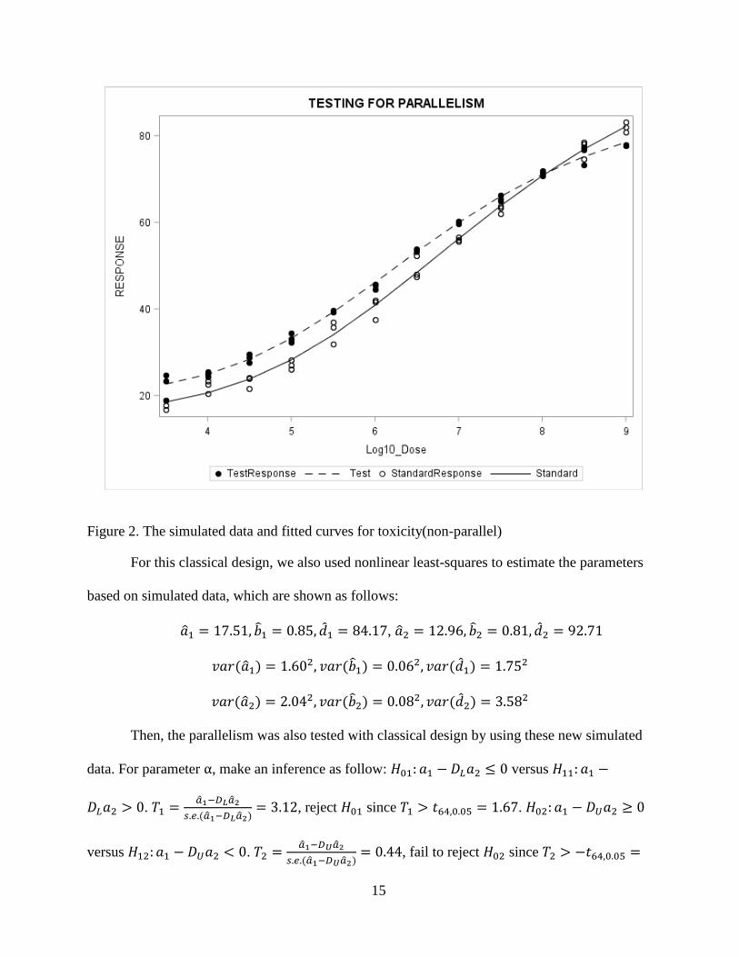
Figure 2. The simulated data and fitted curves for toxicity(non-parallel)

For this classical design, we also used nonlinear least-squares to estimate the parameters

based on simulated data, which are shown as follows:

�̂�1 = 17.51, �̂�1 = 0.85, �̂�1 = 84.17, �̂�2 = 12.96, �̂�2 = 0.81, �̂�2 = 92.71

𝑣𝑎𝑟(�̂�1) = 1.602, 𝑣𝑎𝑟(�̂�1) = 0.062, 𝑣𝑎𝑟(�̂�1) = 1.752

𝑣𝑎𝑟(�̂�2) = 2.042, 𝑣𝑎𝑟(�̂�2) = 0.082, 𝑣𝑎𝑟(�̂�2) = 3.582

Then, the parallelism was also tested with classical design by using these new simulated

data. For parameter α, make an inference as follow: 𝐻01: 𝑎1 − 𝐷𝐿𝑎2 ≤ 0 versus 𝐻11: 𝑎1 −

𝐷𝐿𝑎2 > 0. 𝑇1 =�̂�1−𝐷𝐿�̂�2

𝑠.𝑒.(�̂�1−𝐷𝐿�̂�2)= 3.12, reject 𝐻01 since 𝑇1 > 𝑡64,0.05 = 1.67. 𝐻02: 𝑎1 − 𝐷𝑈𝑎2 ≥ 0

versus 𝐻12: 𝑎1 − 𝐷𝑈𝑎2 < 0. 𝑇2 =�̂�1−𝐷𝑈�̂�2

𝑠.𝑒.(�̂�1−𝐷𝑈�̂�2)= 0.44, fail to reject 𝐻02 since 𝑇2 > −𝑡64,0.05 =

16

−1.67. For parameter b, make an inference as follow: 𝐻01: 𝑏1 − 𝐷𝐿𝑏2 ≤ 0 versus 𝐻11: 𝑏1 −

𝐷𝐿𝑏2 > 0. Since 𝑇1 = 2.29 > 𝑡64,0.05, reject 𝐻01. 𝐻02: 𝑏1 − 𝐷𝑈𝑏2 ≥ 0 versus 𝐻12: 𝑏1 − 𝐷𝑈𝑏2 <

0. Fail to reject 𝐻02 since 𝑇2 = −1.38 > −𝑡64,0.05. For parameter d, make an inference as

follow: 𝐻01: 𝑑1 − 𝐷𝐿𝑑2 ≤ 0 versus 𝐻11: 𝑑1 − 𝐷𝐿𝑑2 > 0. Reject 𝐻01 since 𝑇1 = 2.98 > 𝑡64,0.05.

𝐻02: 𝑑1 − 𝐷𝑈𝑑2 ≥ 0 versus 𝐻12: 𝑑1 − 𝐷𝑈𝑑2 < 0. Reject 𝐻02 since 𝑇2 = −6.61 < −𝑡64,0.05. The

dose-response curves are non-parallel because not all null hypothesizes are rejected.

We got the D-optimal design for the two lines and the modified D-optimal design in

Table 4. In this example, total of 36 responses are used to fit both lines, so the number of

replicated responses of modified D-optimal design 𝑛𝑀 is obtained by the nearest integer of 𝑃𝑀 ∗

36. From Table 4, we found modified D-optimal design has 6 selected dose levels and the

number of replications are varied at each dose levels.

Table 4. D-optimal design for non-parallel example

X Test line

3.5 5.35 7.25 9

𝑃𝑇 0.25 0.25 0.25 0.25

X Control line

3.5 5.56 7.46 9

𝑃𝐶 0.25 0.25 0.25 0.25

X

Modified D-optimal

3.5 5.35 5.56 7.25 7.46 9

𝑃𝑀 0.25 0.125 0.125 0.125 0.125 0.25

𝑛𝑀 9 4 5 5 4 9

Then, D-optimal design was applied to test parallelism. For the test line, use X to generate

𝑌2𝑗𝑘 based on 𝑌1𝑗𝑘 = 16.44 +85.19−16.44

1+exp [0.83(6.35−X)]+ 𝜖1𝑗𝑘. For the standard line, also use X to

obtain response 𝑌′2𝑗𝑘 based on the formula 𝑌′

2𝑗𝑘 = 13.61 +93.01−13.61

1+exp [0.82(6.83−X)]+ 𝜖2𝑗𝑘. Estimated

parameters were obtained, which are as follows:

17

�̂�1 = 14.34, �̂�1 = 0.76, �̂�1 = 87.05, �̂�2 = 12.86, �̂�2 = 0.76, �̂�2 = 95.24

𝑣𝑎𝑟(�̂�1) = 1.452, 𝑣𝑎𝑟(�̂�1) = 0.052, 𝑣𝑎𝑟(�̂�1) = 1.632

𝑣𝑎𝑟(�̂�2) = 1.062, 𝑣𝑎𝑟(�̂�2) = 0.042, 𝑣𝑎𝑟(�̂�2) = 2.012

Test the parallelism using this simulated data. For parameter α, make an inference as

follow: 𝐻01: 𝑎1 − 𝐷𝐿𝑎2 ≤ 0 versus 𝐻11: 𝑎1 − 𝐷𝐿𝑎2 > 0. 𝑇1 = 2.41, reject 𝐻01 since 𝑇1 >

𝑡58,0.05 = 1.67. 𝐻02: 𝑎1 − 𝐷𝑈𝑎2 ≥ 0 versus 𝐻12: 𝑎1 − 𝐷𝑈𝑎2 < 0.𝑇2 = −0.88, fail to reject 𝐻02

since 𝑇2 > −𝑡58,0.05 = −1.67. For parameter b, make an inference as follow: 𝐻01: 𝑏1 − 𝐷𝐿𝑏2 ≤

0 versus 𝐻11: 𝑏1 − 𝐷𝐿𝑏2 > 0. Reject 𝐻01 since 𝑇1 = 2.58 > 𝑡58,0.05.𝐻02: 𝑏1 − 𝐷𝑈𝑏2 ≥ 0 versus

𝐻12: 𝑏1 − 𝐷𝑈𝑏2 < 0. Reject 𝐻02 since 𝑇2 = −2.65 < −𝑡58,0.05. For parameter d, make an

inference as follow: 𝐻01: 𝑑1 − 𝐷𝐿𝑑2 ≤ 0 versus 𝐻11: 𝑑1 − 𝐷𝐿𝑑2 > 0. Reject 𝐻01 since 𝑇1 =

4.74 > 𝑡58,0.05. 𝐻02: 𝑑1 − 𝐷𝑈𝑑2 ≥ 0 versus 𝐻12: 𝑑1 − 𝐷𝑈𝑑2 < 0. Reject 𝐻02 since 𝑇2 =

−10.69 < −𝑡58,0.05. So the dose-response curves are non-parallel based on the fact that not all

the null hypothesis components are rejected. The results are summarized in Table 5.

As seen from Table 5, based on the results of the proposed test, the toxicity assay with

two designs both do not provide compelling evidence that the response profiles are in fact

parallel. While comparing the t value with critical value (𝑡58,0.05 = 1.67), it appears that the

slopes and the plateaus are practically equivalent, and thus that the response profiles may be

considered parallel. What’s more, the fact that absolute t value for D-optimal design is always

larger and it shows that it benefits the experimenter more for improving the precision of the

assay.

In first example, inspection of Figure 1 suggests that the response profiles are

approximately parallel. Testing parallelism with the two design methods both indicated that

response lines are parallel. In contrast to the preceding example, the plot does give some

18

indication of non-parallel the second example response profiles, as the horizontal distance

between the test observations and the standard observations appears to decrease somewhat as the

response level increases. In order to validate the outperformance of the modified optimal design

on the IUT test, we conduct simulation studies under several different scenarios.

Table 5. T value results for the two examples

Parameter Estimate SE T value for test

using 𝐷𝐿

T value for test

using 𝐷𝑈

Ten-dose bioassay(parallel) with classical design

𝑎1 2.08 0.09 3.58 -2.94

𝑎2 2.06 0.11

𝑏1 -1.45 0.05 6.32 -3.10

𝑏2 -1.34 0.04

𝑑1 10.04 0.11 14.34 -16.77

𝑑2 10.15 0.09

Ten-dose bioassay(parallel) with modified D-optimal design

𝑎1 1.98 0.03 4.11 -5.02

𝑎2 2.06 0.09

𝑏1 -1.41 0.03 7.60 -4.87

𝑏2 -1.36 0.04

𝑑1 10.21 0.05 29.05 -18.59

𝑑2 9.82 0.08

Toxicity assay (non-parallel) with classical design

𝑎1 17.51 1.60 3.12 0.44

𝑎2 12.96 2.04

𝑏1 0.85 0.06 2.29 -1.38

𝑏2 0.81 0.08

𝑑1 84.17 1.75 2.98 -6.61

𝑑2 92.71 3.58

Toxicity assay (non-parallel) with modified D-optimal design

𝑎1 14.34 1.45 2.41 -0.88

𝑎2 12.86 1.06

𝑏1 0.76 0.05 2.58 -2.65

𝑏2 0.76 0.04

𝑑1 87.05 1.63 4.74 -10.69

𝑑2 95.24 2.01

19

4. SIMULATION STUDY

Previous section shows some insight of the benefit of using D-optimal design for the IUT

test. To assess more precise properties of the D-optimal design over the classical design method

for testing the parallelism, we performed a simulation study based on the same simulation set-up

in Jonkman and Sidik, 2009. The paper conduct simulation studies for testing parallelism under 5

different scenarios:

1. A case set 𝑎1 = 2.02, 𝑏1 = −1.42, 𝑐1 = 2.31, 𝑑1 = 10.12 for the test preparation,

and 𝑎2 = 2.04, 𝑏2 = −1.35, 𝑐2 = 2.59, 𝑑2 = 9.86 for the standard preparation. The curves for

the test and standard preparations are approximately parallel: that is, a case in which all three

ratios are within the 𝐷𝐿𝑎𝑛𝑑 𝐷𝑈. For this, 𝑎1, 𝑏1, 𝑐1, 𝑑1, 𝑎2, 𝑏2, 𝑐2, 𝑑2are set equal to the parameter

estimates from the example of section 3.

2. A case set 𝑎1 = 2.0, 𝑏1 = −1.4, 𝑐1 = 2.3, 𝑑1 = 10.0 for the test preparation, and 𝑎2 =

2.0, 𝑏2 = −1.4, 𝑐2 = 2.6, 𝑑2 = 10.0 for the standard preparation. The curves are exactly parallel,

and the only difference is the potency. Values 𝑎1, 𝑏1, 𝑐1, 𝑑1, 𝑎2, 𝑏2, 𝑐2, 𝑑2 are close to those from

the example of section 3.


2.0, 𝑏2 = −1.2, 𝑐2 = 2.6, 𝑑2 = 10.0 for the standard preparation. The ratios for the plateaus and

the slope are all on the boundary for the equivalence test: that is, 𝑎1

𝑎2= 𝐷𝐿 = 0.8,

𝑏1

𝑏2= 𝐷𝑈 =

1.25, and 𝑑1

𝑑2= 𝐷𝐿 = 0.8.


2.0, 𝑏2 = −1.4, 𝑐2 = 2.6, 𝑑2 = 10.0 for the standard preparation. The ratio of the lower plateaus

20

is outside the equivalence limits for the IUT (𝑎1

𝑎2< 𝐷𝐿), but the slopes and the upper plateaus are

equal.


2.0, 𝑏2 = −1.16, 𝑐2 = 2.6, 𝑑2 = 10.0 for the standard preparation. The ratio of the slopes is

outside the equivalence limits for the IUT (𝑏1

𝑏2> 𝐷𝑈), but both plateaus are equal.

At the first part, we considered the classical design in Table 1 to simulate the responses.

Next, tested whether the dose-response curves are parallelism or not separately by IUT. Then we

run this 10000 times to calculate the power of detecting the parallelism via IUT. The

investigation was conducted in the same way for the above five cases.

At the second part, repeated all the steps in the previous part using the modified D-

optimal design instead of the standard design. The "VNM" package in R was performed to obtain

multiple-objective optimal design. The MOPT function was used to maximize the optimality

criterion and verify the optimality of the generated design using the General Equivalence

Theorem (See Hyun, Wong and Yang).

All the obtained D-optimal designs and the modified D-optimal design for each case are

given in Table 6, 7, 8, 9, and 10.

Table 6. Modified D-optimal design for two lines in case 1

X Control line

1 1.88 1.89 2.95 4

𝑃𝐶 0.25 0.08 0.17 0.25 0.25

X Test line

1 1.99 3.08 4

𝑃𝑇 0.25 0.25 0.25 0.25

X Modified D-

optimal

1 1.88 1.89 1.99 2.95 3.08 4

𝑃𝑀 0.25 0.04 0.085 0.125 0.125 0.125 0.25

𝑛𝑀 7 1 3 4 4 3 8

21


X Control line

1 1.88 2.95 4

𝑃𝐶 0.25 0.25 0.25 0.25

X Test line

1 2.01 3.08 4

𝑃𝑇 0.25 0.25 0.25 0.25

X

Modified D-optimal

1 1.88 2.01 2.95 3.08 4

𝑃𝑀 0.25 0.125 0.125 0.125 0.125 0.25

𝑛𝑀 7 4 4 4 3 8


X Control line

1 1.88 2.93 4

𝑃𝐶 0.25 0.25 0.25 0.25

X Test line

1 1.97 3.1 4

𝑃𝑇 0.25 0.25 0.25 0.25

X

Modified D-optimal

1 1.88 1.97 2.93 3.1 4

𝑃𝑀 0.25 0.125 0.125 0.125 0.125 0.25

𝑛𝑀 7 4 4 4 3 8


X Control line

1 1.88 2.95 4

𝑃𝐶 0.25 0.25 0.25 0.25

X Test line

1 2.01 3.08 4

𝑃𝑇 0.25 0.25 0.25 0.25

X

Modified D-optimal

1 1.88 2.01 2.95 3.08 4

𝑃𝑀 0.25 0.125 0.125 0.125 0.125 0.25

𝑛𝑀 7 4 4 4 3 8

22


X Control line

1 1.88 2.93 4

𝑃𝐶 0.25 0.25 0.25 0.25

X Test line

1 1.96 3.1 4

𝑃𝑇 0.25 0.25 0.25 0.25

X

Modified D-optimal

1 1.88 1.96 2.93 3.1 4

𝑃𝑀 0.25 0.125 0.125 0.125 0.125 0.25

𝑛𝑀 7 4 4 4 3 8

The results of the simulations are shown in Table 11. For each test and each simulation

case, the table value is power of detecting parallelism, which is the proportion of times among

the 10,000 replicates that each test resulted in a declaration of parallelism. In case 1, the response

curves are not exactly parallel but they are well within the equivalence limits, so we argue that

they are approximately parallel. In this case, when the standard deviation of the two preparations

was high, the classical design declared parallelism relatively rarely (16.89%), while the D-

optimal design with the same test method, declared parallelism a majority of the time (85.14%).

Also, it’s true that the null hypotheses are easily rejected when the standard deviation is small.

That is simulated data were closely distributed around the mean value and didn't change a lot.

However, we could note that for a given value of σ, the proportion of declaring parallelism of D-

optimal design was always greater than that of classical design. So, whatever the sigma is high or

low, it always showed that the D-optimal design provides the preferred inference.

In case 2, the response curves are exactly parallel, and only the potency differs. In this

case, the test with D-optimal design declared parallelism between 88.14% and 99.98% of the

time. Because the null hypothesis for the test is true in this case, this means that the test

maintained a rejection rate in a high level. For the both design approaches, the percentage of

declaring parallelism increased as the standard deviation decreased. However, for standard

23

design, the proportion of rejecting hypothesizes decreased more greatly (from 87.62% to

20.53%). Overall, the results from cases 1 and 2 suggest that tests to establish parallelism with

classical design may be more sensitive to the standard deviation of the data than the tests with D-

optimal design. Even for small σ, still D-optimal design performs much better than classical

design.

In case 3, the ratios of the slopes and the lower and upper plateaus were all set on the

boundary of the equivalence limits. For this case, the tests with D-optimal design never declared

parallelism for any of the 10,000 simulation replicates, regardless of the value of standard

deviation. Similarly, the tests with classical design almost never declared parallelism in this case.

Since the null hypothesis is true in this case, this represents an empirical type I error rate of zero.

The results confirm that changing design approach would not affect the rejection ratio when the

dose-response curves are not parallelism.

In case 4, the ratio of the lower plateaus was set just outside the equivalence limits (𝑎1

𝑎2=

0.75), while the slopes and the upper plateaus were equal. Similarly, in case 5 the ratio of the

slopes was outside the equivalence limits (𝑏1

𝑏2= 1.29), but the upper and lower plateaus were

equal. For both these cases, the both tests seldom declared parallelism regardless of the value of

standard deviation, with a maximum rate of only 0.45% for classical design and 0.47% for D-

optimal design. Since null hypothesis is true in this case, the proportions are less than type I error

rates (0.05).

Overall, the simulation results indicate that the IUT with the modified D-optimal design

for equivalence works better in all cases than with the classical design. The modified D-optimal

design appears to be clearly more effective in the cases illustrated by the examples: precise

assays where the true response curves are approximately or exactly parallel, and assays where

24

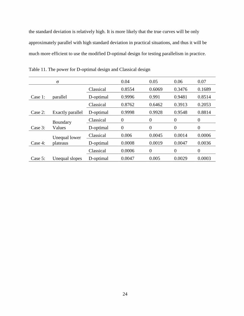
the standard deviation is relatively high. It is more likely that the true curves will be only

approximately parallel with high standard deviation in practical situations, and thus it will be

much more efficient to use the modified D-optimal design for testing parallelism in practice.

Table 11. The power for D-optimal design and Classical design

σ 0.04 0.05 0.06 0.07

Case 1: parallel

Classical 0.8554 0.6069 0.3476 0.1689

D-optimal 0.9996 0.991 0.9481 0.8514

Case 2: Exactly parallel

Classical 0.8762 0.6462 0.3913 0.2053

D-optimal 0.9998 0.9928 0.9548 0.8814

Case 3:

Boundary

Values

Classical 0 0 0 0

D-optimal 0 0 0 0

Case 4:

Unequal lower

plateaus

Classical 0.006 0.0045 0.0014 0.0006

D-optimal 0.0008 0.0019 0.0047 0.0036

Case 5: Unequal slopes

Classical 0.0006 0 0 0

D-optimal 0.0047 0.005 0.0029 0.0003

25

5. SUMMARY

In this article, the problem of testing the parallelism of the response curves for a test

preparation and a standard preparation using the 4PL model was discussed. we argued that the

problem may be more accurately detected by IUT with implementing the D-optimal design. This

result is obtained through comparing the ratio of rejecting null hypothesis, which can be readily

constructed using the output from standard nonlinear regression software. The IUT was easily

implemented by using a sequence of one-sided approximate t-tests, and rejecting the null

hypothesis established evidence in favor of practically parallel response curves.

D-optimal design minimizes the variance of parameter estimated, so it appeared to be

clearly more effective. The simulation results suggested that the modified D-optimal design

indeed provides precise results of testing parallelism in the situations that the true response

curves are indeed exactly or approximately parallel. The classical design does not help very

much for reducing the variance of estimating the parameters while the D-optimal design does.

The classical design becomes more problematic when there is large variance in the dataset. In the

simulation cases where the true response curves were clearly nonparallel, both designs failed to

support parallelism the vast majority of the time. As we have noted before, approximately

parallel lines with high standard deviation are more likely to be tested in practice and this study

suggests to use that the modified D-optimal design can be employed for testing parallelism in

real bioassay.

A potential question is that we just used one test method to compare the D-optimal design

and the classical design. Thus, further study is recommended to contrast the two designs in other

testing methods, such F test or chi-square test.

26

REFERENCES

Berger, R. L. (1982). Multiparameter hypothesis testing and acceptance sampling.

Technometrics 24:295–300.

Berger, R. L., Hsu, J. C. (1996). Bioequivalence trials, intersection-union tests, and equivalence

confidence sets. Statist. Sci. 11:283–319.

Callahan, J. D., Sajjadi, N. C. (2003). Testing the null hypothesis for a specified difference the

right way to test for parallelism. BioProcessing J. March/April:71–77.

Casella, G., Berger, R. L. (1990). Statistical Inference. Belmont, CA: Duxbury Press.

Finney, D. J. (1976). Radioligand assay. Biometrics 32:721–740.

Dykstra, O. (1971), “The Augmentation of Experimental Data to Maximize |X′X|,”

Technometrics, 13, 682488.

Gottschalk, P. G., Dunn, J. R. (2005). Measuring parallelism, linearity, and relative potency in

bioassay and immunoassay data. J. Biopharm. Statist. 15:437–463.

Hauck, W. W., Capen, R. C., Callahan, J. D., De Muth, J. E., Hsu, H., Lansky, D., Sajjadi, N. C.,

Seaver, S. S., Singer, R. H., Weisman, D. (2005). Assessing parallelism prior to determining

relative potency. PDA J. Pharm. Sci. Technol. 59:127–137.

Kpamegan, E. P. (2005). A comparative study of statistical methods to assess dilutional

similarity. BioPharm Inter. 18(10):60–63.

Li, G. and Majumdar, D. (2007), D-optimal designs for logistic models with three and four

Parameters, Journal of Statistical Planning and Inference, 138 (2008) 1950–1959.

Hebble, T. L., and Mitchell, T. J. (l972), I “‘Repairing’ Response Surface Designs,”

Technornetrics, 14, 767-779.

Hyun, S. W., Wong, W. K. and Yang Y.(2018), VNM: An R Package for Finding Multiple-

Objective Optimal Designs for the 4-Parameter Logistic Model, Journal of Statistical

Software, DOI: 10.18637/jss.v083.i05.

Jeffrey N. Jonkman & Kurex Sidik (2009) Equivalence Testing for Parallelism in the Four-

Parameter Logistic Model, Journal of Biopharmaceutical Statistics, 19:5, 818-837.

Toby J. Mitchell (2000), An Algorithm for the Construction of “D-Optimal” Experimental

Designs, Technometrics, 42:1, 48-54.

Mitchell, T. J. (I 972), “An Algorithm for the Construction of ‘D-Optimal’ Experimental

Designs, Applied to First-Order Models,” ORNL-4777, Oak Ridge National Laboratory.

27

Mitchell, T. J., and Miller, F. L., Jr. (1970), “Use of ‘Design Repair’ to Construct Designs for

Special Linear Models,” in Mathematical Division Annual Progress Report (ORNL-466l),

Oak Ridge National Laboratory.

Wynn, H. P. (l970), “The Sequential Generation of D-Optimum Experimental Designs,” The

Annals of Mathematical Statistics, 41, 1655-1664.

V.V. Fedorov, Theory of Optimal Experiments, Academic Press, 1972.

V.V. Fedorov, and P. Hackl, Model-Oriented Design of Experiments, Springer, New York, 1997.

S.W. Hyun, and W.K. Wong, Multiple-Objective Optimal Designs for Studying the Dose

Response Function and Interesting Dose Levels, Int J Biostat. 2015 Nov, DOI: 10.1515/ijb-

2015-0044.

J.M. McGree, J.A. Eccleston, and S.B. Duffull, Compound Optimal Design Criteria for

Nonlinear Models, Journal of Biopharmaceutical Statistics. 18 (2008), pp. 646-661.

F. Pukelsheim, Optimal Design of Experiments, Society for Industrial and Applied Mathematics

(SIAM), Philadelphia, PA, 2006

28

APPENDIX A. R CODES FOR T-VALUES OF CLASSICAL DESIGN

Y<-function(par,x,e){

n<-length(x)

Y<-rep(0,n)

for(i in 1:n){

Y[i]<-par[1]+(par[4]-par[1])/(1+exp(par[2]*(par[3]-x[i])))+e[i]}

return(Y)}

# ten-dosebioassay

pa1<-c(2.02,-1.42,2.31,10.12)

pa2<-c(2.04,-1.35,2.59,10.12)

x11<-seq(1.1,3.8,0.3)

px1<-rep(x11,3)

pe1<-rnorm(30,0,0.04)

y11<-Y(pa1,px1,pe1) #ten-dose test

pe2<-rnorm(30,0,0.04)

y12<-Y(pa2,px1,pe2) #ten-dose control

m<-nls(y11~a+(d-a)/(1+exp(b*(c-px1))),start=list(a=2.02,b=-1.42,c=2.31,d=10.12))

(tm<-summary(m))

n<-nls(y12~a+(d-a)/(1+exp(b*(c-px1))),start=list(a=2.04,b=-1.35,c=2.59,d=9.86))

(tn<-summary(n))

#toxicityassay

pa3<-c(16.44,0.83,6.35,85.19)

pa4<-c(13.61,0.82,6.83,93.01)

x21<-seq(3.5,9,0.5)

px2<-c(x21,x21,x21)

e31<-rnorm(12,0,1.4)

e32<-rnorm(12,0,1.4)

e33<-rnorm(12,0,1.4)

pe3<-c(e31,e32,e33)

y21<-Y(pa3,px2,pe3) #toxicity control

e41<-rnorm(12,0,1.4)

e42<-rnorm(12,0,1.4)

e43<-rnorm(12,0,1.4)

pe4<-c(e41,e42,e43)

y22<-Y(pa4,px2,pe4) #toxicity test

p<-nls(y21~a+(d-a)/(1+exp(b*(c-px2))),start=list(a=16.44,b=0.83,c=6.35,d=85.19))

(tp<-summary(p))

q<-nls(y22~a+(d-a)/(1+exp(b*(c-px2))),start=list(a=13.61,b=0.82,c=6.83,d=93.01))

(tq<-summary(q))

Dl=0.8

Du=1.25

T1=seq(3)

T2=seq(3)

for(i in 1:4){

29

T1[i]=(abs(tm$coefficients[i,1])-

Dl*abs(tn$coefficients[i,1]))/sqrt(tm$coefficients[i,2]^2+Dl^2*tn$coefficients[i,2]^2)


Du*abs(tn$coefficients[i,1]))/sqrt(tm$coefficients[i,2]^2+Du^2*tn$coefficients[i,2]^2)

}

T1

T2

TT1=seq(3)

TT2=seq(3)

for(i in 1:4){

TT1[i]=(tp$coefficients[i,1]-

Dl*tq$coefficients[i,1])/sqrt(tp$coefficients[i,2]^2+Dl^2*tq$coefficients[i,2]^2)

TT2[i]=(tp$coefficients[i,1]-

Du*tq$coefficients[i,1])/sqrt(tp$coefficients[i,2]^2+Du^2*tq$coefficients[i,2]^2)

}

TT1

TT2

30

APPENDIX B. R CODES FOR T-VALUES OF D-OPTIMAL DESIGN

library("VNM")

Design1<- MOPT(LB = 1, UB = 4, P = c(2.02, 8.10, 10.07, -1.42),lambda = c(1,0), delta = -1,

r = 30, verbose = TRUE)

Design2<- MOPT(LB = 1, UB = 4, P = c(2.04, 7.82, 13.33, -1.35),lambda = c(1,0), delta = -1,

r = 30, verbose = TRUE)

summary(Design1)

summary(Design2)

library("VNM")

Design1<- MOPT(LB = 3.5, UB = 9, P = c(16.44, 68.75, 572.49, 0.83),lambda = c(1,0), delta

= 1, r = 36, verbose = TRUE)

Design2<- MOPT(LB = 3.5, UB = 9, P = c(13.61, 79.4, 925.19, 0.82),lambda = c(1,0), delta =

1, r = 36, verbose = TRUE)

summary(Design1)

summary(Design2)

##case2##

Design1<- MOPT(LB = 1, UB = 4, P = c(2, 8, 9.97, -1.4),lambda = c(1,0), delta = -1, r = 30,

verbose = TRUE)


verbose = TRUE)

summary(Design1)

summary(Design2)

##case3##

Design1<- MOPT(LB = 1, UB = 4, P = c(1.6, 6.4, 9.97, -1.5),lambda = c(1,0), delta = -1, r =

30, verbose = TRUE)


verbose = TRUE)

summary(Design1)

summary(Design2)

##case4##

Design1<- MOPT(LB = 1, UB = 4, P = c(1.5, 8.5, 9.97, -1.4),lambda = c(1,0), delta = -1, r =

30, verbose = TRUE)


verbose = TRUE)

summary(Design1)

summary(Design2)

case##case5##


verbose = TRUE)


verbose = TRUE)

summary(Design1)

summary(Design2)

##############################################


31

n<-length(x)

Y<-rep(0,n)

for(i in 1:n){


return(Y)}

# ten-dosebioassay

pa1<-c(2.02,-1.42,2.31,10.12)

pa2<-c(2.04,-1.35,2.59,9.86)

dx1<-c(rep(1,7),rep(1.88,1),rep(1.89,3),rep(1.99,4),rep(2.95,4),rep(3.08,3),rep(4,8))

Dl=0.8

Du=1.25

r_d=0

total=0

t1<-qt(0.05,52,lower.tail = FALSE)

t2<-qt(0.05,52)

e11<-rnorm(20,0,0.04)

e12<-rnorm(20,0,0.04)

e13<-rnorm(20,0,0.04)

pe1<-c(e11,e12,e13)

dy11<-Y(pa1,dx1,pe1) #test

e21<-rnorm(20,0,0.05)

e22<-rnorm(20,0,0.05)

e23<-rnorm(20,0,0.05)

pe2<-c(e21,e22,e23)

dy12<-Y(pa2,dx1,pe2) #control

dm<-nls(dy11~a+(d-a)/(1+exp(b*(c-dx1))),start=list(a=2.02,b=-1.42,c=2.31,d=10.12),control

= list(maxiter = 100))

tdm<-summary(dm)

dn<-nls(dy12~a+(d-a)/(1+exp(b*(c-dx1))),start=list(a=2.04,b=-1.35,c=2.59,d=9.86),control =

list(maxiter = 100))

tdn<-summary(dn)

dT1=seq(4)

dT2=seq(4)

for(i in 1:4){

dT1[i]=(abs(tdm$coefficients[i,1])-

Dl*abs(tdn$coefficients[i,1]))/sqrt(tdm$coefficients[i,2]^2+Dl^2*tdn$coefficients[i,2]^2)


Du*abs(tdn$coefficients[i,1]))/sqrt(tdm$coefficients[i,2]^2+Du^2*tdn$coefficients[i,2]^2)}

if(dT1[1]>t1 & dT1[2]>t1 & dT1[4]>t1 & dT2[1]<t2 & dT2[2]<t2 & dT2[4]<t2){

r_d=r_d+1}

##########################################


n<-length(x)

Y<-rep(0,n)

for(i in 1:n){

32


return(Y)}

# ten-dosebioassay

pa1<-c(16.44,0.83,6.35,85.19)

pa2<-c(13.61,0.82,6.83,93.01)

dx1<-c(rep(3.5,18),rep(5.35,9),rep(5.56,9),rep(7.25,9),rep(7.46,9),rep(9,18))

Dl=0.8

Du=1.25

r_d=0

total=0


t2<-qt(0.05,64)

e11<-rnorm(24,0,1.6)

e12<-rnorm(24,0,1.6)

e13<-rnorm(24,0,1.6)

pe1<-c(e11,e12,e13)

dy11<-Y(pa1,dx1,pe1) #test

e21<-rnorm(24,0,1.6)

e22<-rnorm(24,0,1.6)

e23<-rnorm(24,0,1.6)

pe2<-c(e21,e22,e23)

dy12<-Y(pa2,dx1,pe2) #control

dm<-nls(dy11~a+(d-a)/(1+exp(b*(c-dx1))),start=list(a=16.44,b=0.83,c=6.35,d=85.19),control


tdm<-summary(dm)

dn<-nls(dy12~a+(d-a)/(1+exp(b*(c-dx1))),start=list(a=13.61,b=0.82,c=6.83,d=93.01),control


tdn<-summary(dn)

dT1=seq(4)

dT2=seq(4)

for(i in 1:4){






r_d=r_d+1}

33

APPENDIX C. R CODES FOR POWER OF CLASSICAL DESIGN


n<-length(x)

Y<-rep(0,n)

for(i in 1:n){


return(Y)}

# ten-dosebioassay

pa1<-c(2.02,-1.42,2.31,10.12)

pa2<-c(2.04,-1.35,2.59,10.12)

x11<-seq(1.1,3.8,0.3)

px1<-rep(x11,3)

Dl=0.8

Du=1.25


t2<-qt(0.05,52)

T1=seq(3)

T2=seq(3)

r=0

a=0

total=0

for(j in 1:10000){

pe1<-rnorm(30,0,0.07)


pe2<-rnorm(30,0,0.07)



tm<-summary(m)


tn<-summary(n)

for(i in 1:4){




Du*abs(tn$coefficients[i,1]))/sqrt(tm$coefficients[i,2]^2+Du^2*tn$coefficients[i,2]^2)}

total=total+1

if(T1[1]>t1 & T1[2]>t1 & T1[4]>t1 & T2[1]<t2 & T2[2]<t2 & T2[4]<t2){

r=r+1}

}

(power_no<-r/total)

####################################################################

#case2


n<-length(x)

Y<-rep(0,n)

34

for(i in 1:n){


return(Y)}

# ten-dosebioassay

pa1<-c(2,-1.4,2.3,10)

pa2<-c(2,-1.4,2.6,10)

x11<-seq(1.1,3.8,0.3)

px1<-rep(x11,3)

Dl=0.8

Du=1.25


t2<-qt(0.05,52)

T1=seq(3)

T2=seq(3)

r=0

a=0

total=0

for(j in 1:10000){

pe1<-rnorm(30,0,0.07)


pe2<-rnorm(30,0,0.07)



tm<-summary(m)


tn<-summary(n)

for(i in 1:4){





total=total+1

if(T1[1]>t1 & T1[2]>t1 & T1[4]>t1 & T2[1]<t2 & T2[2]<t2 & T2[4]<t2){

r=r+1}

}

(power_no<-r/total)

####################################################################

#case3


n<-length(x)

Y<-rep(0,n)

for(i in 1:n){


return(Y)}

# ten-dosebioassay

pa1<-c(1.6,-1.5,2.3,8)

35

pa2<-c(2,-1.2,2.6,10)

x11<-seq(1.1,3.8,0.3)

px1<-rep(x11,3)

Dl=0.8

Du=1.25


t2<-qt(0.05,52)

T1=seq(3)

T2=seq(3)

r=0

a=0

total=0

for(j in 1:10000){

pe1<-rnorm(30,0,0.04)


pe2<-rnorm(30,0,0.04)



tm<-summary(m)


tn<-summary(n)

for(i in 1:4){





total=total+1

if(T1[1]>t1 & T1[2]>t1 & T1[4]>t1 & T2[1]<t2 & T2[2]<t2 & T2[4]<t2){

r=r+1}

}

(power_no<-r/total)

####################################################################

#case4


n<-length(x)

Y<-rep(0,n)

for(i in 1:n){


return(Y)}

# ten-dosebioassay

pa1<-c(1.5,-1.4,2.3,10)

pa2<-c(2,-1.4,2.6,10)

x11<-seq(1.1,3.8,0.3)

px1<-rep(x11,3)

Dl=0.8

Du=1.25

36


t2<-qt(0.05,52)

T1=seq(3)

T2=seq(3)

r=0

a=0

total=0

for(j in 1:10000){

pe1<-rnorm(30,0,0.07)


pe2<-rnorm(30,0,0.07)



tm<-summary(m)


tn<-summary(n)

for(i in 1:4){





total=total+1

if(T1[1]>t1 & T1[2]>t1 & T1[4]>t1 & T2[1]<t2 & T2[2]<t2 & T2[4]<t2){

r=r+1}

}

(power_no<-r/total)

####################################################################

#case5


n<-length(x)

Y<-rep(0,n)

for(i in 1:n){


return(Y)}

# ten-dosebioassay

pa1<-c(2,-1.5,2.3,10)

pa2<-c(2,-1.16,2.6,10)

x11<-seq(1.1,3.8,0.3)

px1<-rep(x11,3)

Dl=0.8

Du=1.25


t2<-qt(0.05,52)

T1=seq(3)

T2=seq(3)

r=0

37

a=0

total=0

for(j in 1:10000){

pe1<-rnorm(30,0,0.06)


pe2<-rnorm(30,0,0.06)



tm<-summary(m)


tn<-summary(n)

for(i in 1:4){





total=total+1

if(T1[1]>t1 & T1[2]>t1 & T1[4]>t1 & T2[1]<t2 & T2[2]<t2 & T2[4]<t2){

r=r+1}

}

(power_no<-r/total)

38

APPENDIX D. R CODES FOR POWER OF D-OPTIMAL DESIGN

#case1#


n<-length(x)

Y<-rep(0,n)

for(i in 1:n){


return(Y)}

# ten-dosebioassay

pa1<-c(2.02,-1.42,2.31,10.12)

pa2<-c(2.04,-1.35,2.59,10.12)

dx1<-c(rep(1,7),rep(1.88,1),rep(1.89,3),rep(1.99,4),rep(2.95,4),rep(3.08,3),rep(4,8))

Dl=0.8

Du=1.25

r_d=0

total=0

dT1=seq(4)

dT2=seq(4)


t2<-qt(0.05,52)

for(j in 1:10000){

pe1<-rnorm(30,0,0.07)

dy11<-Y(pa1,dx1,pe1) #ten-dose control

pe2<-rnorm(30,0,0.07)

dy12<-Y(pa2,dx1,pe2) #ten-dose test



tdm<-summary(dm)



tdn<-summary(dn)

for(i in 1:4){





total=total+1


r_d=r_d+1}

}

(power_d<-r_d/total)

########################################################

#case2


n<-length(x)

39

Y<-rep(0,n)

for(i in 1:n){


return(Y)}

# ten-dosebioassay

pa1<-c(2,-1.4,2.3,10)

pa2<-c(2,-1.4,2.6,10)

dx1<-c(rep(1,7),rep(1.88,4),rep(2.01,4),rep(2.95,4),rep(3.08,3),rep(4,8))

Dl=0.8

Du=1.25

r_d=0

total=0

dT1=seq(4)

dT2=seq(4)


t2<-qt(0.05,52)

for(j in 1:10000){

pe1<-rnorm(30,0,0.04)


pe2<-rnorm(30,0,0.04)




tdm<-summary(dm)



tdn<-summary(dn)

for(i in 1:4){





total=total+1


r_d=r_d+1}

}


########################################################

#case3


n<-length(x)

Y<-rep(0,n)

for(i in 1:n){


return(Y)}

# ten-dosebioassay

40

pa1<-c(1.6,-1.5,2.3,8)

pa2<-c(2,-1.2,2.6,10)


Dl=0.8

Du=1.25

r_d=0

total=0

dT1=seq(4)

dT2=seq(4)


t2<-qt(0.05,52)

for(j in 1:10000){

pe1<-rnorm(30,0,0.06)


pe2<-rnorm(30,0,0.06)




tdm<-summary(dm)



tdn<-summary(dn)

for(i in 1:4){





total=total+1


r_d=r_d+1}

}


########################################################

#case4


n<-length(x)

Y<-rep(0,n)

for(i in 1:n){


return(Y)}

# ten-dosebioassay

pa1<-c(1.5,-1.4,2.3,10)

pa2<-c(2,-1.4,2.6,10)


Dl=0.8

Du=1.25

41

r_d=0

total=0

dT1=seq(4)

dT2=seq(4)


t2<-qt(0.05,52)

for(j in 1:10000){

pe1<-rnorm(30,0,0.07)


pe2<-rnorm(30,0,0.07)




tdm<-summary(dm)



tdn<-summary(dn)

for(i in 1:4){





total=total+1


r_d=r_d+1}

}


par(mfrow=c(1,2))

plot(dx1,dy11,col="red")

plot(dx1,dy12,col="green")

########################################################

#case5


n<-length(x)

Y<-rep(0,n)

for(i in 1:n){


return(Y)}

# ten-dosebioassay

pa1<-c(2,-1.5,2.3,10)

pa2<-c(2,-1.16,2.6,10)


Dl=0.8

Du=1.25

r_d=0

total=0

42

dT1=seq(4)

dT2=seq(4)


t2<-qt(0.05,52)

for(j in 1:10000){

pe1<-rnorm(30,0,0.04)


pe2<-rnorm(30,0,0.04)




tdm<-summary(dm)



tdn<-summary(dn)

for(i in 1:4){





total=total+1


r_d=r_d+1}

}

(power_d<-r_d/to

testing parallelism for the four-parameter logistic …

Documents