testing a marine ecosystem model: sensitivity analysis and parameter optimization

Ž .Journal of Marine Systems 28 2001 45–63www.elsevier.nlrlocaterjmarsys

Testing a marine ecosystem model: sensitivity analysis andparameter optimization

Katja Fennel), Martin Losch, Jens Schroter, Manfred Wenzel¨Alfred-Wegener-Institut fur Polar-und Meeresforschung, 27515 BremerhaÕen, Germany¨

Received 1 April 2000; accepted 1 September 2000

Abstract

A data assimilation technique is used with a simple but widely used marine ecosystem model to optimize poorly knownmodel parameters. A thorough analysis of the a posteriori errors to be expected for the estimated parameters was carried out.The errors have been estimated by calculating the Hessian matrices for different problem formulations based on identicaltwin experiments. The error analysis revealed inadequacies in the formulation of the optimization problem and insufficien-cies of the applied data set. Modifications of the actual problem formulation, which improved the accuracy of the estimatedparameters considerably, are discussed.

The optimization procedure was applied to real measurements of nitrate and chlorophyll at the Atlantic Bermuda site. Theparameter optimization gave poor results. We suggest this to be due to features of the ecosystem that are unresolved by thepresent model formulation. Our results emphasize the necessity of an error analysis to accompany any parameteroptimization study. q 2001 Elsevier Science B.V. All rights reserved.

Keywords: Marine ecosystem; Sensitivity analysis; Parameter optimization

1. Introduction

Within the scope of global climate studies, themodeling community is seeking marine ecosystemmodels capable of describing wide regions of theoceans. Models should be robust and behave equallywell in different biogeochemical provinces of theglobal ocean. These range from temperate and highlatitude systems, which may be viewed as a linearfood chain, to oligotrophic systems, characterized by

) Corresponding author. COAS, Oregon State University, 104Ocean Admin. Bldg., Corvallis, OR 97331, USA.

Ž .E-mail address: [email protected] K. Fennel .

high overturning rates and a food net dominated bythe microbial loop. Parameterizations appropriate torepresent these different types of ecosystems areneeded for basin-wide and global ocean models. Theparameters in marine ecosystem models are gener-ally poorly known quantities. This is mainly due tothe fact that the model state variables are highlyintegrated pools that comprise different species,which are affected differently by biotic and abioticchanges in their environment. The model parametersshould represent the integrated behavior of this het-erogenic mixture of species. Furthermore, the pro-portions of the different species contributing to thespecies pool may change in time as ecosystemsrespond to changes in environmental conditions.

0924-7963r01r$ - see front matter q 2001 Elsevier Science B.V. All rights reserved.Ž .PII: S0924-7963 00 00083-X

( )K. Fennel et al.rJournal of Marine Systems 28 2001 45–6346

Thus, the model parameters are not straightforwardto define.

The parameter values are difficult to determine bymeasurements. Single quantities like phytoplanktongrowth rates may be found by laboratory experi-ments. However, these values represent mostly sin-gle species under controlled conditions and theirapplication to the in situ conditions is questionable.Only until recently, the general procedure for settingparameters of ecological models was to use corre-sponding values from former modeling studiesandror fit the model output to observed data bysubjective tuning of the parameters. The employmentof data assimilation techniques seems an attractivealternative, since these methods allow one to settlepoorly known model parameters objectively basedon statistical assumptions about observations of thereal system. Such a parameter estimation is done bycombining the dynamical model and measurementsof the state of the real system. The data assimilationtechnique generally used within the context of pa-

Žrameter optimization is the adjoint method Lawsonet al., 1995, 1996; Schartau et al., 2000; Spitz et al.,

.1998, 2000 . A few studies employ simulated anneal-Ž .ing Hurtt and Armstrong, 1996, 1999; Matear, 1995

Žor a non-linear optimization technique Evans, 1999;.Fasham and Evans, 1995; Prunet et al., 1996a,b to

perform parameter optimizations. The basic idea un-derlying these methods is to vary model parametersuntil the misfit between the dynamical model and thetime-distributed data is minimized, while the modelequations are fulfilled exactly. The general procedureof parameter estimation by the adjoint method is

Ž .discussed in detail by Evensen et al. 1998 .Former assimilation studies demonstrate that the

optimization of ecological parameters is a difficulttask. While the feasibility of the adjoint method torecover model parameters was shown in principle by

Židentical twin experiments Lawson et al., 1996;.Schartau et al., 2000; Spitz et al., 1998 , the applica-

tion to real observations turned out to be problem-Ž .atic. For instance, Fasham and Evans 1995 did not

find a parameter set that would give a good fit to thewhole observation set simultaneously, Prunet et al.Ž .1996a found only a few model parameters to be

Ž .constrained by the data, and Spitz et al. 1998 couldnot estimate the optimal model parameters whenemploying real observations.

Since an optimization procedure can only provideestimates of the parameters in question, we regardstudies of this kind as not complete without ananalysis of the errors of the optimal estimate. Thispaper provides a thorough investigation of the errorsto be expected for the optimal parameter estimates.The important problem of what aspects of the param-eter set are difficult to determine or are not con-strained by the available data is illuminated by anerror analysis. The estimated a posteriori errors in-spire modifications of the problem formulation andreveal the inadequacies in the employed data setsand model formulation. Since the error analysis isbased on a widely used modeling approach, theresults apply to a whole class of presently usedecological models.

The ecological model, the inverse formulation,and the method to obtain the error estimates aredescribed in Section 2. The error analysis is pre-sented and discussed in Sections 3 and 4, respec-tively. An application of the optimization procedureto real observations is performed in Section 5, fol-lowed by its discussion in Section 6. The paperconcludes with Section 7.

2. Method

2.1. The ecological model

The ecosystem model employed in this study is asimple representation of the nitrogen cycle, but nev-ertheless a widely used approach to describe thepelagic system of marine environments. The modelconsists of four partial differential equations thatdetermine the dynamical evolution of the state vari-ables: dissolved inorganic nutrients DIN, phytoplank-ton Phy, zooplankton Zoo and detritus Det. This typeof model is also termed the NPZD-model. Aschematic of the model is given in Fig. 1. NPZD-models are currently used in various spatial resolu-tions ranging from vertically integrated and one-di-

Žmensional models Doney et al., 1996; Evans and.Parslow, 1985; Fennel, 1995 to coupled three-di-

Žmensional models Fennel, 1999; Oschlies and.Garcon, 1998, 1999; Palmer and Totterdell, 1999 .

While the conceptual structure of the ecological partof all of these models is very similar, slight differ-

( )K. Fennel et al.rJournal of Marine Systems 28 2001 45–63 47

Fig. 1. Schematic of the NPZD-model.

ences occur in the explicit mathematical formulationof the process parameterizations. The latter are em-pirical and thus depend to some extent on the per-sonal choice of the modeler.

This study is based on a vertically integratedformulation of the model, that is, the state variablesare assumed to be homogenously distributed over themixed layer. The evolution of the mixed layer iscalculated from prescribed daily mixed layer depthsŽ .MLD . The prescribed mixed layer depths are takenfrom a simulation of the general circulation model

Ž .described by Drange 1996 . The circulation modelis a version of the Miami Isopycnic Coordinate

Ž . Ž .Ocean Model MICOM Bleck et al., 1992 employ-ing the mixed layer parameterization of GasparŽ .1988 and forced with ECMWF wind stresses, heatfluxes and solar radiation. The positive change of the

qŽ .mixed layer depth h t determines the rate ofnutrient entrainment into the mixed layer from greaterdepths. It is given by

hq t smax h t ,0 ,Ž . Ž .Ž .dMLD

where h t s . 1Ž . Ž .d t

The phytoplankton growth rate g depends on theP

supply of dissolved inorganic nutrients DIN accord-ing to a linear Michaelis–Menten kinetic and on the

Ž .availability of photosynthetically active light F I .The growth rate is given by

DIN 1 MLDg I ,DIN sm P F I d z ,Ž . Ž .HP P k qDIN MLD 0N

2Ž .

where m is the maximum phytoplankton growthP

rate, k the half-saturation concentration for nutrientN

uptake and I the depth dependent radiation. TheŽ .photosynthesis to light relationship PI-curve is de-

Ž .termined following Evans and Parslow 1985

aPparIF I s . 3Ž . Ž .

2 2 2 2(m qa par IP

Here a represents the initial slope of the PI-curveand par is a constant determining the fraction ofincident light that is available for photosynthesis.The phytoplankton loss terms comprise grazing byzooplankton g and linear metabolical losses due toZ

the constant respiration and mortality rates l andPN

l , respectively. The zooplankton grazing is repre-PD

sented by a squared Michaelis–Menten response

Phy 2

g sm , 4Ž .Z Z 2k qPhyP

where m is the maximum grazing rate and k theZ P

half-saturation concentration for phytoplankton in-gestion. Zooplankton exudation is described by aconstant rate l while zooplankton mortality isZN

assumed to be quadratically dependent on the zoo-plankton standing stock, that is l Zoo2. DetrialZD

particles are remineralized in the mixed layer at aconstant rate l and sink out of the mixed layer atDN

a constant velocity w .D

With these definitions, the model equations readexplicitly

dPhysg Phyyg Zooyl Phyyl PhyP Z PN PDd t

mqhq tŽ .y Phy 5Ž .

MLD

dZoo h tŽ .2sg Zooyl Zooyl Zoo y ZooZ ZN ZDd t MLD

6Ž .


dDINsyg Phyql Phyql Zooql DetP PN ZN DNd t

mqhq tŽ .q N MLDyDIN 7Ž .Ž .slopeMLD

dDET2sl Phyql Zoo yl DetPD ZD DNd t

mqhq t qwŽ . Dy Det. 8Ž .

MLD

Ž . Ž .The last terms of Eqs. 5 – 8 account for thephysical processes of nutrient entrainment, dilution

Ž .and mixing Evans and Parslow, 1985 . Dissolvedinorganic nutrients, phytoplankton and detritus aremixed at the constant mixing rate m across the lowerface of the mixed layer and are diluted if the mixedlayer deepens by hq. Zooplankton Zoo is assumed tomaintain its position in the mixed layer and thus isdiluted if the mixed layer deepens and concentratedif the mixed layer depth decreases. Nutrients areentrained from greater depths during deepening ofthe mixed layer. The deep nutrient concentrations aredescribed by assuming a linear increase N withslope

Ž .depth Hurtt and Armstrong, 1996 . The model pa-rameters are given in Table 1.

The model presented here is very similar to theŽ .formulations of Oschlies and Garcon 1998, 1999

Ž .and Doney et al. 1996 who also employ a linearMichaelis–Menten response for phytoplankton

growth and a squared response for zooplankton graz-ing. The zooplankton mortality is represented by aquadratic rate in their models as well.

2.2. The inÕerse formulation

The idea underlying the inverse parameter opti-mization is to combine the simulated model dynam-ics with the available information about the realsystem, that is a set of observations. Based on theassumption that the validity of the model parametersdepends on the match between the observed data andthe model equivalents of these data, we search for aset of parameters that provides the best fit of themodel dynamics to the observations. The search foran optimal parameter set is performed by minimizinga cost function that measures the misfit between thedata and the model equivalents of the data in a leastsquares sense. The cost function is generally of theform

2™obs sim1 X yX pŽ .i i™F p s , 9Ž .Ž . Ý ž /2 sii

™where p represents the vector of the unknown pa-rameters. The misfit between the observations X obs

i

and the corresponding simulated model variables

Table 1Initial guess of model parameters

Parameter Symbol Initial value Unity1Phytoplankton maximum growth rate m 1.0 dayP

y3Half-saturation value for phytoplankton growth k 0.25 mmol N mNy1Phytoplankton mortality rate l 0.05 dayPDy1Phytoplankton respiration rate l 0.05 dayPNy1Zooplankton maximum growth rate m 2.0 dayZ

2 y6Ž .Half-saturation value for zooplankton growth k 0.5 mmol N mPy3 y1 y1Ž .Zooplankton mortality rate l 0.05 mmol N m dayZD

y1Zooplankton exudation rate l 0.05 dayZNy1Remineralisation rate l 0.05 dayDN

y2 y1 y1Ž .Initial slope of the PI-curve a 0.025 W m dayPhotosynthetic active fraction of light par 0.43 dimensionless

y1Detritus sinking rate w 1.0 m dayDy1Cross thermocline mixing m 0.25 m day

y4Slope of nitrate concentration below the thermocline N 0.016 mmol N mslope

ŽThe initial parameter guess agrees with values in common use compare Oschlies and Garcon, 1999; Doney et al., 1996; Fasham et al.,.1990 .


™sim Ž .X p is weighted by the inverse of the assumed ai

priori error s . A minimization algorithm is appliedi

to search for the minimum of the cost function.Every minimization step requires the computation ofthe gradient of the cost function with respect to themodel parameters. Basically, the parameter optimiza-tion is an iteration of the following three steps.

Ž .A A forward model integration: the forwardŽ .model described in Section 2.1 calculates the evo-

lution of the model state variables in time. Note thatthe initial conditions and the physical forcing areprescribed. Thus, the model dynamics are solelydetermined by the choice of the model parameters.The parameters are called independent variables orcontrol variables in this context while the modelstate variables are dependent variables.

Ž .B An integration of the adjoint model: the ad-joint model calculates the gradient of the cost func-tion with respect to the model parameters. We usedthe Tangent linear and Adjoint Model CompilerŽ .TAMC , a source-to-source translator for FOR-

Ž .TRAN programs Giering, 1997 , as a convenienttool to obtain the adjoint model code.

Ž .C An optimization step: a minimization is per-formed in the direction of the gradient of the costfunction that was computed in step B. We appliedthe quasi-Newton method implemented in the

ŽM1QN3 routine of the MODULOPT library Gilbert.and Lemarechal, 1989 .´

This procedure is iterated until the gradient of thecost function is sufficiently small. Since the model isnon-linear it is desirable to start the iteration near theglobal minimum in order to prevent the descentalgorithm from being caught in a local minimum.Since this can be hard to judge in practice, it maybecome necessary to start a number of minimizationsfrom different initial parameter sets.

2.3. The Hessian matrix

Important aspects of the problem formulation canbe revealed by an investigation of the Hessian matrixof the cost function. Near the global minimum, theinverse of the Hessian matrix provides a good ap-proximation of the covariance matrix for the inde-

Ž .pendent model parameters Thacker, 1989 . The con-dition number of the Hessian, which is defined as theratio of its largest to its smallest eigenvalue, deter-

mines the rate of convergence of the minimizationalgorithm and indicates how singular the problem is.For large condition numbers, the matrix is ill condi-tioned and nearly singular, whereas values close tounity characterize a well-conditioned matrix. Theinverse eigenvalues of the Hessian are the errors ofcombinations of the estimated model parameters.These combinations are determined by the corre-sponding eigenvectors. The product of the eigenvec-tors and corresponding eigenvalues are also calledparameter resolution. In the case of large inverseeigenvalues, meaning large uncertainties, some ofthe model parameter combinations can only poorlybe determined by the data.

The Hessian of the cost function can be approxi-mated by independently perturbing the control vari-ables by a small amount and calculating the gradientof the cost function for each perturbation. The ele-ments of the Hessian result in

1™h s EF pqD p rEpŽ .ži j j i2D pj

™yEF pyD p rEp . 10Ž .Ž . /j i

Since this finite difference method can be depen-dent on the choice of the D p ’s, we have chosen toj

Ž .use the TAMC Giering, 1997 to calculate the Hes-sian of the tangent linear model. Since the modelunder consideration is non-linear, it is crucial tocompute the Hessian at the global minimum of thecost function, that is for the optimal parameter set.We ensure this by conducting the sensitivity analysisfor identical twin experiments, where syntheticallyproduced data are taken as observations. In this case,the optimal parameter set is known, since it was usedto generate the synthetic data set.

3. Sensitivity experiments

The sensitivity analysis is based on identical twinexperiments at the Bermuda station at 31840XN64810XW, which is part of the U.S. JGOFS program.A synthetic data set was created by monthly sam-pling of the simulated model course from January

Ž .1989 to December 1992 Fig. 2 , using the initial


ŽFig. 2. Simulated model course at the Bermuda station. A synthetic data set was produced by monthly sampling circles, asterisks and.crosses represent the synthetic data . The errorbars represent the assumed a priori errors s .i

parameter values given in Table 1. The inverseformulation of the parameter estimation problem isobtained by defining the cost function

M1 2™ obs simF p s DIN yDINŽ .Ž . Ý22sDIN is1

M1 2obs simq Phy yPhyŽ .Ý22sPhy is1

M1 2obs simq Zoo yZoo . 11Ž . Ž .Ý2ž /2sZoo is1

Please note that the third term on the right handside of the equation accounts for zooplankton dataand is only relevant for the experiments E4 and E7Ž . 2Table 2 . The weights 1rs are chosen to be equali

for the dissolved inorganic nutrients, phytoplanktonŽ y3and zooplankton s s0.1 mmol N m , isDIN,i

.Phy, Zoo . The Hessian of F is calculated accordingto the procedure described in Section 2.3.

3.1. Experiment E1— assimilation of nitrate and phy-toplankton at the Bermuda station

Ž .For the first assimilation experiment E1, Table 2we employ monthly nitrate and phytoplankton data.This corresponds to the data availability from the

Ž .Bermuda Atlantic Time-series Study BATS . TheHessian matrix for this formulation was calculated.Its condition number is 9.0=107, indicating a nearlysingular Hessian and an ill-conditioned problem for-

Ž .mulation. The a posteriori errors given in Table 3are enormous especially for the initial slope of thePI-curve a , the fraction of photosynthetically activeradiation par and the parameters related to zooplank-ton, that is the maximum grazing rate m , the half-Z

saturation constant for ingestion k and the zoo-P

plankton mortality l . The parameter resolution,ZD

given by the eigenvectors and eigenvalues of theHessian, is shown in Fig. 3. The eigenvectors be-longing to the smallest eigenvalues represent combi-nations of parameters that either cannot be deter-mined at all or have large uncertainties. By far thesmallest eigenvalue is l s1.4=10y6. The corre-1


Table 2Description of the twin experiments E1–E8

Experiment Comments

E1 Monthly nitrate and phytoplankton data at the BATS site were employed. All 12 biological model parametersare included in the inversion.

E2 Monthly nitrate and phytoplankton data at the BATS site were employed. par and the maximum grazing rate mZ

were kept fixed.E3 Monthly nitrate and phytoplankton data at the BATS site were employed. par, m and the maximum growth rate mZ P

were kept fixed.E4 Monthly nitrate, phytoplankton and zooplankton data at the BATS site were employed. par, m and m were kept fixed.Z P

E5 Monthly nitrate, phytoplankton and nitrate uptake data at the BATS site were employed. par, m and m were kept fixed.Z PŽ .compare E3

E6 Monthly nitrate and phytoplankton data at the North Atlantic site were employed. par and m were kept fixed.ZŽ .in analogy to E2

E7 Monthly nitrate, phytoplankton and zooplankton data at the North Atlantic site were employed. par and mZ

were kept fixed.E8 Monthly nitrate and phytoplankton data at the BATS and the North Atlantic sites were employed. par and mZ

Ž .were kept fixed. combination of E2 and E6

™sponding eigenvector Õ has significant contribu-1

tions only for the light parameters a and par. Thus,all information on the independent component of a

™and par is represented by Õ . As the corresponding1

eigenvalue l is extremely small, the independent1

component of a and par cannot be determined byassimilation of the data or, in other words, a and parcannot be determined independently. Inspection ofthe model equations reveals that a and par enter the

Žmodel only in multiplicative combination compareŽ ..Eq. 3 . Thus, the indefiniteness of the combination

of a and par results from the model formulation of

the light-curve and the dependence of both parame-ters is not surprising. However, since a and parenter the model only in multiplicative combination,all we need to optimize is their product. By denoting

Ž .a :saPpar we reformulate Eq. 3 toˆ

a IˆF I s . 12Ž . Ž .

2 2 2(m qa IˆP

In all following experiments, we restrict the opti-mization to the combination a . This is realizedˆ

Table 3Condition numbers and a posteriori errors for experiments E1–E8

Exp. E1 E2 E3 E4 E5 E6 E7 E87 4 4 4 4 5 5 4Cond. 9.0=10 1.2=10 1.1=10 1.7=10 1.1=10 1.6=10 1.2=10 3.0=10

Post.m 2.5 2.4 – – – 0.62 0.45 0.37P

k 2.2 2.2 1.4 1.2 1.4 1.3 1.1 0.36N

l 3.6 3.6 3.4 2.8 3.4 2.4 1.7 1.2PD

l 6.1 5.9 5.5 4.4 5.5 4.3 4.7 2.1PN

m 49 – – – – – – –Z

k 53 1.4 1.4 0.84 1.4 2.9 1.4 1.1P

l 12 10 10 3.7 10 3.4 1.2 1.8ZD

l 2.3 1.5 1.5 0.87 1.5 2.8 1.3 1.0ZN

l 4.2 4.2 4 3.6 4.0 4.8 3 2.2DN

a 596 1.8 1.5 1.3 1.5 2.2 2.3 0.97par 596 – – – – – – –w 5.7 4.7 4.5 2.9 4.5 3.2 1.5 1.3D

All errors are scaled by the initial parameter values.


Fig. 3. Parameter resolution for experiment E1. Monthly measurements of nitrate and phytoplankton concentrations were employed.


practically by fixing par on the initial guess andseeking only a .

The second smallest eigenvalue is l s1.9=2™y410 . The corresponding eigenvector Õ combines2

information on zooplankton parameters, basically theŽ .grazing parameters m maximum grazing rate andZ

Žk half-saturation constant for phytoplankton inges-P.tion , with a small contribution from the zooplankton

mortality l . The combination of m and k isZD Z P

only poorly constrained by the data, or in otherwords their a posteriori errors are large. A possiblereason might be that the simulated model course isalmost stationary, that is, the state variables changeonly slightly with time. The phytoplankton standingstocks in the subtropical North Atlantic remain at alow and relatively constant level compared to re-gions with a more pronounced seasonal cycle, suchas the midlatitudes of the North Atlantic, which arecharacterized by a strong increase of nutrient concen-trations during deep winter mixing events and highplankton standing stocks during the typical springand autumn blooms. In accordance with observationsŽ .Michaels and Knap, 1996 , the simulated phyto-plankton concentrations at the BATS station remainbetween 0.1 and 0.2 mmol N my3 and the modelcourse shows no high amplitude signals. Conse-quently, the grazing rates that correspond to the datacover only a small range of the parameter spaceclose to the stationary point. In this case, the grazingrates that correspond to the AmeasuredB data arelimited to the initial slope of the grazing response.

ŽNo data points lie within the saturation range Fig..4 . The information contained in the data does not

suffice to estimate both the half-saturation constantand the saturation rate at the same time. The sameproblem applies to the determination of the growth

Ž .parameters m maximum growth rate and kP NŽ .half-saturation concentration for nitrate uptake . Thesimulated growth rates cover a slightly broader rangethan the grazing rates, but are still limited to the

Ž .initial slope of the growth response Fig. 4 .

3.2. Experiments E2 and E3— a modification of theproblem formulation

As a result of experiment E1, the maximum graz-ing rate and the half-saturation constant for phyto-plankton ingestion cannot be estimated simultane-ously. We believe this to be due to the fact that

grazing rates are restricted to a small part of thegrazing response function. Thus, the applied data setdoes not contain enough information to determineboth parameters simultaneously. The same problemapplies to the phytoplankton growth function wheredata are restricted to the initial slope of the growthresponse. The maximum growth rate and the half-saturation constant for nutrient uptake may not beestimated at the same time.

To test this hypothesis we check first if the condi-tioning of the problem improves when we restrict thesearch to the half-saturation concentrations and sup-pose we know the maximum grazing and maximumgrowth rates. In experiment E2 only the maximumgrazing rate m was kept fixed at the optimal value.Z

This modification improved the condition numberconsiderably to 1.2=104. Also the a posteriori er-

Ž .rors are smaller for most of the parameters Table 3 .In particular the errors of k and a are reduced byP

two and three orders of magnitude, respectively. Inexperiment E3, the maximum growth rate m wasP

held constant as well. This leads again to a smallimprovement of the condition number and the aposteriori errors. However, as the errors range from140% for k to 1000% for the zooplankton mortalityP

l , they are still far from being acceptable.ZD

The parameter resolution for E3 is shown in Fig.5. Note that the first four eigenvectors that corre-spond to the smallest eigenvalues are very similar inexperiments E2 and E3. The most uncertain parame-

™ter combination Õ contains information only on the1

mortality rate of zooplankton l while contribu-ZD

tions for l are negligible in all other eigenvectors.ZD

Thus, l is independent of the other parametersZD

and practically not constrained by the data. This isconsistent with the outstanding large a posteriorierror of 1000% for l . We assume that this is dueZD

to lack of data.The schematic of the model state variables and

Ž .flows Fig. 1 illustrates that fluxes between phyto-plankton, zooplankton and detritus are not directlyconstrained by the data set used. The model allowsdifferent pathways to close the nitrogen cycle, namelyphytoplankton™ zooplankton™detritus™nitrogenand phytoplankton™detritus™nitrogen. The recy-cling pathways are likely to be unconstrained ifneither zooplankton nor detritus information is avail-able. The conditioning of the problem might improve


Fig. 4. Zooplankton grazing and phytoplankton growth response. Actual growth and grazing rates corresponding to the synthetic monthlyDIN Phy 2

Ž .data points are calculated as m and m , respectively. Values are displayed for the Bermuda station asterisks and aP Z 2k qDIN k qPhyN PŽ .North Atlantic station open circles , which we refer to in Section 3.4.

if other types of measurements, e.g. observations ofzooplankton or fluxes, are incorporated. This consid-

eration motivates the following experiments E4 andE5.


Fig. 5. Parameter resolution for experiment E3. Monthly measurements of nitrate and phytoplankton concentrations were employed. par, mZ

and m were kept fixed.P


3.3. Experiments E4 and E5— additional employ-ment of zooplankton and primary production data

We suppose that the large a posteriori errors inexperiment E3 are due to gaps in the employed dataset, which comprises only nitrogen and phytoplank-ton data. In experiment E4, we modify E3 by theadditional inclusion of zooplankton data. A remark-able increase in the accuracy of the estimated param-eters is achieved by the incorporation of zooplanktondata. The a posteriori errors improved in particularfor the zooplankton related parameters k , l andP ZN

l , but also for all the other parameters. Note thatZD

in spite of the decreased errors, the condition numberof the Hessian is slightly larger than for E3. Thismeans that the new data does not add information tothe poorly determined combination of parameterswhich is represented by the smallest eigenvalue.Instead, the new data increase the precision of thealready well determined parameter combinations. Interms of the Hessian spectrum, the largest eigenval-ues are raised even further, thereby increasing therange of the spectrum.

Several parameter optimization studies employmeasurements of primary production in addition tonitrate and chlorophyll data. Experiment E5 is per-formed to assess how this additional informationaffects the accuracy of the parameter estimation.Experiment E5 compares to E3, differing from E3only in the inclusion of the actual nitrate uptake ratemeasurements, that is g Phy, which corresponds toP

the use of primary production data in parameteroptimization assimilations. The inclusion of the up-take rate data did not improve the accuracy of theparameters. This result suggests that measurementsof the flux of nitrogen from the inorganic nitrogenpool to phytoplankton does not add any information

to the system that is not already contained in theinorganic nitrogen and phytoplankton data.

3.4. Experiments E6, E7 and E8— assimilation at theNorth Atlantic station at 478N 208W

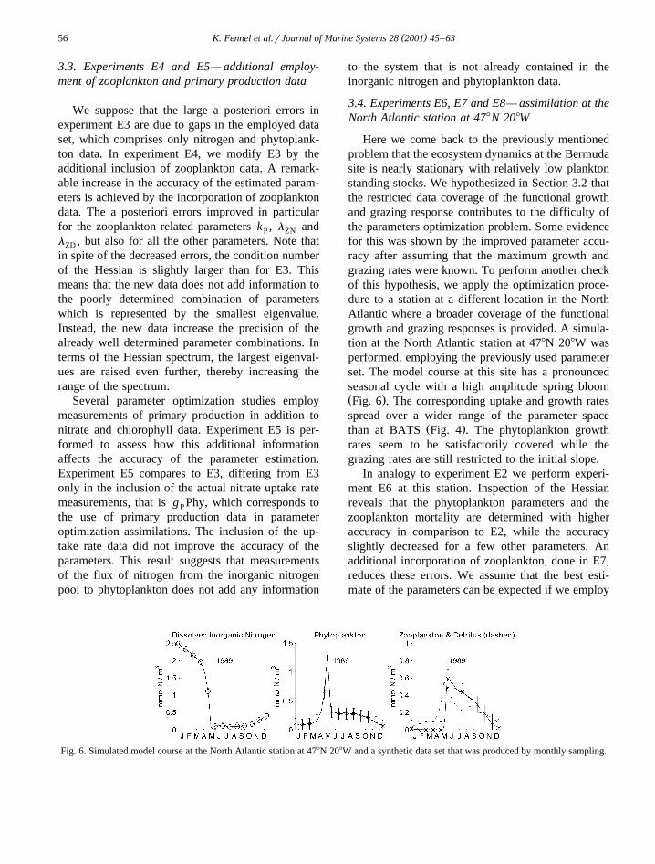
Here we come back to the previously mentionedproblem that the ecosystem dynamics at the Bermudasite is nearly stationary with relatively low planktonstanding stocks. We hypothesized in Section 3.2 thatthe restricted data coverage of the functional growthand grazing response contributes to the difficulty ofthe parameters optimization problem. Some evidencefor this was shown by the improved parameter accu-racy after assuming that the maximum growth andgrazing rates were known. To perform another checkof this hypothesis, we apply the optimization proce-dure to a station at a different location in the NorthAtlantic where a broader coverage of the functionalgrowth and grazing responses is provided. A simula-tion at the North Atlantic station at 478N 208W wasperformed, employing the previously used parameterset. The model course at this site has a pronouncedseasonal cycle with a high amplitude spring bloomŽ .Fig. 6 . The corresponding uptake and growth ratesspread over a wider range of the parameter space

Ž .than at BATS Fig. 4 . The phytoplankton growthrates seem to be satisfactorily covered while thegrazing rates are still restricted to the initial slope.

In analogy to experiment E2 we perform experi-ment E6 at this station. Inspection of the Hessianreveals that the phytoplankton parameters and thezooplankton mortality are determined with higheraccuracy in comparison to E2, while the accuracyslightly decreased for a few other parameters. Anadditional incorporation of zooplankton, done in E7,reduces these errors. We assume that the best esti-mate of the parameters can be expected if we employ

Fig. 6. Simulated model course at the North Atlantic station at 478N 208W and a synthetic data set that was produced by monthly sampling.


the North Atlantic and the Bermuda data sets simul-taneously. This is done in E8. In E8 we achieved thebest accuracy of all experiments. The most uncertainparameters with uncertainties of over 200% are thephytoplankton mortality l and the remineraliza-PN

tion rate l .DN

4. Discussion of the sensitivity analysis

A sensitivity analysis was conducted to assess thecapability of the adjoint method to optimize theecological model parameters. The parameter opti-mization may be difficult for a variety of reasons.Generally, difficulties might be associated with theformulation of the inverse problem that is to besolved and with the numerical approach to its solu-

Ž .tion Thacker, 1989 . Difficulties might stem fromthe model formulation itself. The data may be an-other source of difficulty, i.e. they may be inade-quate to determine the model parameters, therebycausing the least squares problem to be singular orill-posed. By investigating the Hessian matrix of theproblem we tried to sort out the different sources ofdifficulty. The initial formulation of the problemturned out to be ill-posed with parameter combina-tions that could be estimated only with large uncer-tainties and with expected slow convergence of theminimization algorithm. One difficulty obviouslyarose from the formulation of the model itself. Pa-rameters that enter the numerical model formulationonly as a product of each other cannot be estimatedindependently. In our first model formulation, theinitial slope of the PI-curve a and the fraction ofphotosynthetically active radiation par occur as aproduct only. The uncertainty related to the unfavor-able formulation can easily be circumvented by re-stricting the optimization to the combination of bothparameters.

Furthermore, we found evidence that the informa-tion provided by the available measurements is notsufficient to constrain all parameters. Two majorreasons cause the inadequacy of the data set. Firstly,the data set is restricted to only nitrate and phyto-plankton observations. That turned out to be respon-sible for the poor accuracy of the parameters relatedto zooplankton behavior and the remineralizationprocess, since two alternative unconstrained cycling

pathways exist. Experiments with additional incorpo-ration of zooplankton data displayed an improvementof the accuracy of these parameters. Secondly, itmatters which region of the parameter space is cov-ered by the data. Observations of an ecosystemwhich is close to equilibrium like at the Bermudasite provides less information on model parametersthan ecosystems with pronounced seasonal changes.In particular the growth and grazing rates at theBermuda site are restricted to the initial slope of thefunctional response and do not constrain the satura-tion concentrations. The inclusion of observationsfrom a North Atlantic site with a clear yearly cycleprovided a better coverage of the parameter spaceand increased the accuracy of the estimated parame-ters.

5. Parameter optimization at the Bermuda station

We performed a parameter optimization by assim-ilating data of the Bermuda Atlantic Time-series

Ž . Ž .Study BATS Michaels and Knap, 1996 . Biweeklyto monthly measurements of nitrate, nitrite andchlorophyll within the period January 1989 to Octo-ber 1992 were employed. The observed data havebeen transformed as follows to serve as counterpartsto the simulated variables. Nitrate and nitrite wereadded to be comparable to the dissolved inorganicnitrogen pool. Ammonium concentrations had to beneglected since ammonium concentrations are notmeasured on a regular basis. Chlorophyll measure-ments are generally assumed to represent the phyto-plankton standing stock and were compared to themodel phytoplankton. The necessary conversion from

w y3 x wchlorophyll mg chl m to phytoplankton mmol Ny3 xm is problematic, since the intracellular ratios of

chlorophyll to carbon and chlorophyll to nitrogen areknown to vary considerably. The chlorophyll to car-bon ratio varies not only for different species butalso due to changes in environmental conditions,e.g., differences in the ambient nutrient or lightclimate. Recently, different parameterizations for avariable chlorophyll to carbon ratio have been sug-

Žgested in the context of parameter optimization Hurttand Armstrong, 1996, 1999; Schartau et al. 2000;

.Spitz et al. 2000 while other studies rely on aŽconstant average conversion ratio Evans, 1999;


Fasham and Evans, 1995; Prunet et al., 1996a,b;.Spitz et al., 1998 . We assume a constant ratio ofŽ .y1c s1.2 mg chl mmol N in this study. The1

vertically distributed data were integrated over theprescribed mixed layer depth to correspond to thesimulated mixed layer mean concentrations.

The sensitivity analysis discussed in Section 3revealed that not all parameters can be determinedby the optimization. Therefore, we restrict the in-verse formulation to 8 of the 12 biological modelparameters. The fraction of the photosyntheticallyactive radiation par was fixed. An inclusion of par inthe inversion is not appropriate since it enters themodel formulation only in combination with the

Ž .initial slope of the PI-curve a see Section 3.1 , butalso not necessary since par is a relatively wellknown parameter. Furthermore, the maximum growthand grazing rates m and m were excluded fromP Z

the parameter estimation, since the nearly stationaryecosystem dynamics at the Bermuda station does notallow the optimization of the half-saturation concen-trations and the corresponding maximum rates simul-

Ž .taneously see Section 3.2 . The twin experimentsrevealed that the zooplankton mortality rate l isZD

practically not constrained if only nitrate and phyto-plankton observations are employed. Since no zoo-plankton data are available for our optimizationproblem, we also fixed the zooplankton mortality.par, m , m and l are fixed to the initial guessP Z ZD

Ž .values Table 1 .The cost function of the optimization problem has

been defined as

1 2obs™ simF p s Ý NO qNO yDINŽ .Ž . Ž .3 222sDIN

1 2obs simq Ý Chl rc yPhyŽ .122sPhy

™qF p 13Ž .Ž .prior

1™ 0 2Ž . Ž Ž . Ž ..where F p s Ý ln p r p .prior i i i2

The first two terms of the right hand side of Eq.Ž .13 represent the model-data misfit for the inorganicnitrogen pool and the phytoplankton standing stockrespectively. The term F was added to penalizeprior

estimates outside of the acceptable parameter range.Ž .As pointed out by Evensen et al. 1998 , any avail-

able a priori information on the parameters should beused to constrain the problem. Unfortunately, we donot have much a priori information, but we know atleast that negative parameter values are meaningless.Consequently we have chosen F such that nega-prior

tive parameter values are avoided. Otherwise, nega-tive parameter values might occur during gradientdescent steps of the minimization algorithm. Thevariance s 2 is based on estimated standard devia-DIN

Žtions of the measurements for nitrate s s0.08NO 3y3 . Žmmol N m and nitrite s s0.02 mmol NNO 2

y3 . Ž .m Grasshoff et al., 1999 . A standard deviationof s s0.1 mmol N my3 is assumed for phyto-Phy

plankton measurements. Since the cost function inŽ .Eq. 14 differs from the cost function used for the

Ž Ž .twin experiments described above Eq. 11 in Sec-.tion 3 , the error estimates for the twin experiments

cannot be compared directly to the estimates for thereal data experiment in this section. We have per-formed an additional twin experiment in analogy to

Ž .Section 3 employing the cost function 14 to obtainthe error estimates that directly correspond to theestimated errors for the real data experiment.

5.1. Results of the optimization

Our first guess for the model parameters is theŽpreviously used parameter set compare Tables 1 and

.4 , which is based on parameter values in commonuse. The model simulation based on the first guessparameter set leads to relatively good agreementbetween the simulated course and the observed inor-

Ž .ganic nitrogen and chlorophyll data Fig. 7 . Thesimulated course lies within the error range for mostof the measurements. There are mainly three ob-served features that are not reproduced by the model.The model does not capture the increased nitrogenconcentrations during the deep mixing periods inwinter, especially in January, February and March1992. The simulated chlorophyll concentrations aresystematically higher than the observations duringsummer, and the simultaneous increase of observedchlorophyll concentrations and inorganic nitrogenfrom late autumn to early winter is not captured bythe model.

The optimized parameter values with their a pos-teriori error estimates and the a posteriori errors for


Ž .Fig. 7. Simulated model course solid and dashed lines at the Bermuda station based on the initial guess parameter set in comparison to theŽ .observed data circlesrasterisks with a priori error bars.

the twin experiment are given in Table 4. The opti-mization changed the half-saturation concentration

for nitrate uptake k and the phytoplankton respira-N

tion rate l most notably, with a decrease in k byPN N

Table 4ŽModel parameters: initial guess, optimal estimate with absolute a posteriori errors and relative a posteriori errors scaled by the optimal

.estimate , also shown are the relative errors of the corresponding twin experiment

Parameter Initial Relative Optimal estimate with Relative error ofvalue error absolute errors twin experiments

y3k 0.25 0.81 0.043"0.035 mmol N m 0.55Ny1l 0.05 0.65 0.084"0.055 day 0.50PDy1l 0.05 0.58 0.116"0.065 day 0.81PN

2 y6Ž .k 0.5 0.54 0.275"0.145 mmol N m 0.63Py1l 0.05 0.42 0.036"0.015 day 0.65ZNy1l 0.05 0.61 0.089"0.055 day 0.81DN

y2 y1 y1Ž .a 0.025 0.27 0.025"0.007 W m day 0.27y1w 1.0 0.28 0.97"0.27 m day 0.28D


a factor of 5 and an increase in l by a factor of 2.PN

The other parameters differ by about 50% or lessfrom their initial guess. The model course, resultingfrom the optimal estimate, is shown in Fig. 8. Only aslight improvement of the match between observa-tions and simulation is evident. The increase ofinorganic nitrogen during the mixing event in Jan-uary–February 1992 is more pronounced in the opti-mized simulation. The mismatch between model anddata during summer periods improved slightly. Themost obvious change between the initial and theoptimized simulations is a dramatic increase in zoo-plankton concentrations, which are not constrainedby any data.

An assessment of the a posteriori errors was doneby calculating the Hessian matrix of the tangent

linear model for the optimal parameter set accordingto Section 2.3. The resulting condition number of theproblem is 435. This relatively small value indicatesthat the problem with prior knowledge term is wellconditioned. The condition number of the corre-sponding twin experiment is small as well with avalue of 106. The significant reduction of the condi-tion number compared to Section 3 is due to theprior knowledge term F , which obviously regu-prior

larizes the problem. The prior knowledge also re-Žduces the a posteriori errors compare errors in Table

.4 with previous results given in Table 3 , but mosterrors still range around 50% of the initial parametervalue. Note that most of the optimized values differfrom their initial guess by less than their a posteriorierror estimate.

Fig. 8. Simulated model course at the Bermuda station based on the optimal parameter set in comparison to the observed data.


6. Discussion of the parameter optimization

The parameter optimization did not improve thematch between the model and the observations no-tably. The simulation that is based on the new pa-rameter set is very similar to the initial simulation interms of nitrate and phytoplankton, which were con-strained by observed data. The most obvious reduc-tion of the model-data misfit was achieved for nitro-gen concentrations during a deep mixing event inJanuary–March 1992. The zooplankton course, whichwas not constrained by any observations, changedremarkably. This is consistent with the large uncer-tainties of the zooplankton parameters given by thesensitivity analysis, since large uncertainties of pa-rameters allow large variations of these parametersduring the optimization procedure.

There may be different reasons for the poor resultof the optimization. Firstly, the course of the ecolog-ical variables depends largely on the physical forcingconditions, namely the mixed layer depth, whichwere prescribed. In terms of the parameter estimationprocedure, prescribing the physical forcing is equiva-lent to the assumption that the forcing is correct.Thus, the optimization parameters are adjusted insuch a way that they correct for any errors related tophysical forcing conditions that influence the ecolog-ical state variables. Secondly, the model is zero-di-mensional, which is clearly an oversimplification.All the ecological state variables are considered asaverage concentrations over the mixed layer. Thismisconstrues important features of the ecosystem atBermuda, e.g. the deep chlorophyll maximum persis-tent below the mixed layer. A third potential reasonfor errors is the omission of advective transportprocesses in the model. Since mesoscale eddies in-fluence the Bermuda region, advection is likely to beimportant.

However, a major concern goes beyond the issuesrelated to spatial resolution and external forcing. Thewhole optimization has to be questioned if the modeldoes not represent the observed system appropri-ately. The parameter optimization is bound to fail ifthe model does not resolve the processes whichdetermine the observed features. The application ofthe optimization procedure to a specific model and acorresponding set of observations relies on the inher-ent assumption that the simulated and observed sys-

tems are consistent. The simultaneous increase of theobserved chlorophyll and nitrate concentrations dur-ing deep mixing periods in winter is an example ofsuch an unresolved feature, which is not possible tograsp with the present model formulation. It mightbe related to variations in the chlorophyll to nitrateratio that are not resolved by the present model.Furthermore, the microbial loop, which is not in-cluded in the present model that is rather designed asa representation of the linear food chain, is probablyan important factor.

7. Conclusions

A sensitivity analysis should be an integral part ofany attempt to optimize the parameters of ecologicalmodels. Sensitivity experiments are extremely help-ful in revealing problems that contribute to the diffi-culty of parameter optimization and formulation of awell-conditioned problem. There are sources of errorrelated to an inappropriate formulation of the prob-lem that can be circumvented. Furthermore, the sen-sitivity experiments can identify gaps or inadequa-cies in the applied data set. A data set can beinsufficient because information on certain parts ofthe model is missing or because of poor coverage ofthe parameter space. In this context the sensitivityanalysis goes beyond the rather technical issue offormulating the optimization problem as it providesfeedback to observationalists about how to designfield campaigns and sampling strategies that allowone to constrain numerical models.

The application of the optimization procedure toreal data at the Bermuda station brought up a morefundamental problem. The parameter estimation gavepoor results that we believe to be due to an inconsis-tency of the present model formulation with theecological system under observation. This outcomeemphasizes the important role that parameter opti-mization methods can play in testing model assump-tions during model development. Since it is notpossible to verify the theoretical assumptions under-

Ž .lying a model in principle Oreskes et al., 1994 and,moreover, ecological modeling is mostly heuristicand in a comparably premature state, the modeldevelopment has to be viewed as an iterative processwhere the refutation of model assumptions leads to


Ž .the development of new hypothesies Loehle, 1983 .In this respect, the systematic test of parameterchoices by the application of optimization techniquescan be extremely powerful.

Acknowledgements

We are grateful to J.Chr. Gilbert and Ch.Lemarechal for providing the MODULOPT mini-´mization routine M1QN3 and to Ralf Giering formaking the TAMC compiler available. SvetlanaLoza’s double checking of the calculations was highlyappreciated. We thank Yvette Spitz for her criticalcomments and Jasmine Bartlett for reviewing themanuscript. This work has been supported by the ECMAST-III project DIADEM under contract MAS3-CT98-0167.

References

Bleck, R., Rooth, C., Hu, D., Smith, L.T., 1992. Salinity-driventhermohaline transients in a wind- and thermohaline-forcedisopycnic coordinate model of the North Atlantic. Journal ofPhysical Oceanography 22, 1486–1515.

Doney, S.C., Glover, D.M., Najjar, R.G., 1996. A new coupled,one-dimensional model for the upper ocean: applications to

Ž .the JGOFS Bermuda Atlantic Time-series Study BATS site.Deep-Sea Research II 43, 591–624.

Drange, H., 1996. A 3-dimensional isopycnic coordinate model ofthe seasonal cycling of carbon and nitrogen in the AtlanticOcean. Physics and Chemistry of the Earth 21, 503–509.

Evans, G.T., 1999. The role of local models and data sets in theJoint Global Ocean Flux Study. Deep-Sea Research I 46,1369–1389.

Evans, G.T., Parslow, J.S., 1985. A model of annual planktoncycles. Biological Oceanography 3, 327–347.

Evensen, G., Dee, D., Schroter, J., 1998. Parameter estimation in¨Ž .dynamical models. In: Chassignet, E.P., Verron, J. Eds. ,

Ocean Modeling and Parameterizations. NATO ASI.Fasham, M.J.R., Evans, G.T., 1995. The use of optimization

techniques to model marine ecosystem dynamics at the JGOFSstation at 47 deg N 20 deg W. Philosophical Transactions ofthe Royal Society of London B 348, 203–209.

Fasham, M.J.R., Ducklow, H.W., McKelvie, S.M., 1990. A nitro-gen-based model of plankton dynamics in the oceanic mixed-layer. Journal of Marine Research 48, 591–639.

Fennel, K., 1999. Convection and the timing of phytoplanktonspring blooms in the western Baltic Sea. Estuarine, Coastaland Shelf Science 49, 113–128.

Fennel, W., 1995. A model of the yearly cycle of nutrients andplankton in the Baltic Sea. Journal of Marine Systems 6,313–329.

Gaspar, P., 1988. Modeling the seasonal cycle of the upper ocean.Journal of Physical Oceanography 18, 161–180.

Giering, R., 1997. Tangent Linear and Adjoint Model Compiler.User’s Manual. MIT, http:rrpuddle.mit.edur; ralfrtamc.

Gilbert, J.C., Lemarechal, C., 1989. Some numerical experiments´with variable storage quasi-Newton algorithms. MathematicalProgramming 45, 407–435.

Grasshoff, K.M., Kremling, K., Ehrhardt, M., 1999. Methods ofSeawater Analysis. 3rd edn. Wiley-VCH, Weinheim.

Hurtt, G.C., Armstrong, R.A., 1996. A pelagic ecosystem modelcalibrated with BATS data. Deep-Sea Research II 43, 653–683.

Hurtt, G.C., Armstrong, R.A., 1999. A pelagic ecosystem modelcalibrated with BATS and OWSI data. Deep-Sea Research I46, 27–61.

Lawson, L.M., Spitz, Y.H., Hofmann, E.E., Long, R.B., 1995. Adata assimilation technique applied to a predator–prey model.Bulletin of Mathematical Biology 57, 593–617.

Lawson, L.M., Hofmann, E.E., Spitz, Y.H., 1996. Time seriessampling and data assimilation in a simple marine ecosystemmodel. Deep-Sea Research II 43, 625–651.

Loehle, C., 1983. Evaluation of theories and calculation tools inecology. Ecological Modelling 19, 239–247.

Matear, R.J., 1995. Parameter optimization and analysis of ecosys-tem models using simulated annealing: a case study at stationP. Journal of Marine Research 53, 571–607.

Michaels, A.F., Knap, A.H., 1996. Overview of the U.S. JGOFSBermuda Atlantic Time-series Study and the Hydrostation Sprogram. Deep-Sea Research II 43, 157–198.

Oreskes, N., Shrader-Frechette, K., Belitz, K., 1994. Verification,validation, and confirmation of numerical models in earthsciences. Science 263, 641–646.

Oschlies, A., Garcon, V., 1998. Eddy induced enhancement ofprimary production in a model of the North Atlantic Ocean.Nature 394, 266–269.

Oschlies, A., Garcon, V., 1999. An eddy-permitting coupledphysical–biological model of the North Atlantic: 1. Sensitivityto advection numerics and mixed layer physics. Global Bio-geochemical Cycles 13, 135–160.

Palmer, J.R., Totterdell, I.J., 1999. Production and export in aŽglobal ocean ecosystem model. Deep-Sea Research sub-

.mitted .Prunet, P., Minster, J.F., Ruiz-Pino, D., 1996a. Assimilation of

surface data in a one-dimensional physical–biogeochemicalmodel of the surface ocean: 1. Method and preliminary results.Global Biogeochemical Cycles 10, 111–138.

Prunet, P., Minster, J.F., Echevin, V., Dadou, I., 1996b. Assimila-tion of surface data in a one-dimensional physical–biogeo-chemical model of the surface ocean: 2. Adjusting a simpletrophic model to chlorophyll, temperature, nitrate, and pCO2data. Global Biogeochemical Cycles 10, 139–158.

Schartau, M., Oschlies, A., Willebrand, J., 2000. Parameter esti-mation of a zero-dimensional ecosystem model applying the

Ž .adjoint method. Deep-Sea Research II in press .


Spitz, Y.H., Moisan, J.R., Abbott, M.R., 2000. Configuring anecosystem model using data from the Bermuda-Atlantic Time

Ž . Ž .Series BATS . Deep-Sea Research II in press .Spitz, Y.H., Moisan, J.R., Abbott, M.R., Richman, J.G., 1998.

Data assimilation and a pelagic ecosystem model: parameteri-

zation using time series observations. Journal of Marine Sys-tems 16, 51–68.

Thacker, W.C., 1989. The role of the Hessian in fitting models tomeasurements. Journal of Geophysical Research C 94, 6177–6196.

testing a marine ecosystem model: sensitivity analysis and parameter optimization

Documents