UniMAP

Chapter 1Digital Signal Processing

Introduction

EKT 353/3

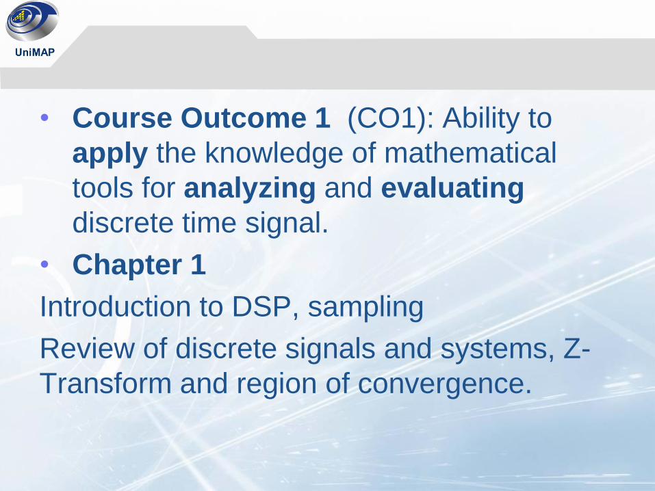
• Course Outcome 1 (CO1): Ability to

apply the knowledge of mathematical

tools for analyzing and evaluating

discrete time signal.

• Chapter 1

Introduction to DSP, sampling

Review of discrete signals and systems, Z-

Transform and region of convergence.

Outline

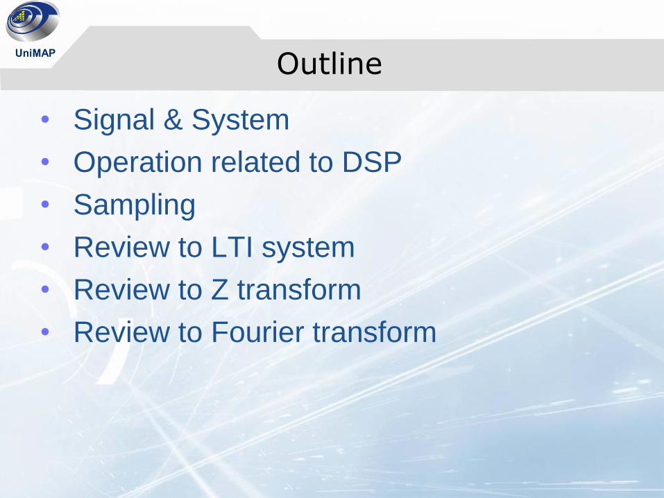
• Signal & System

• Operation related to DSP

• Sampling

• Review to LTI system

• Review to Z transform

• Review to Fourier transform

Signal and System

Signal

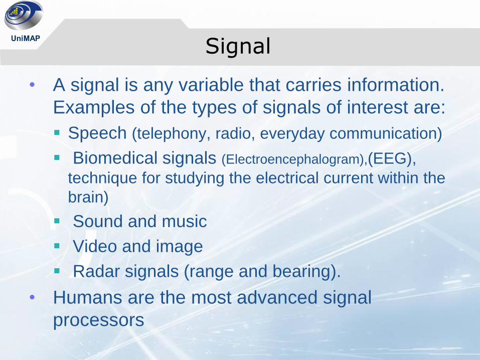
• A signal is any variable that carries information.

Examples of the types of signals of interest are:

Speech (telephony, radio, everyday communication)

Biomedical signals (Electroencephalogram),(EEG),

technique for studying the electrical current within the

brain)

Sound and music

Video and image

Radar signals (range and bearing).

• Humans are the most advanced signal

processors

Signal

• Signals are patterns of variation of physical

quantities such as temperature, pressure,

voltage, brightness, etc.

• Two different standpoints of signal:

The time domain.

• the trace on an oscilloscope where the vertical deflection is

the signals amplitude, and the horizontal deflection is the

time variable.

The frequency domain.

• trace on a spectrum analyzer, where the horizontal deflection

is the frequency variable and the vertical deflection is the

signals amplitude at that frequency.

Signal Types

• Analog signals: continuous in time and amplitude

Example: voltage, current, temperature,…

• Digital signals: discrete both in time and amplitude

Example: attendance of this class, digitizes analog signals,…

• Discrete-time signal: discrete in time, continuous in amplitude

Example:hourly change of temperature in Austin

• Theory for digital signals would be too complicated

Requires inclusion of nonlinearities into theory

• Theory is based on discrete-time continuous-amplitude signals

Most convenient to develop theory

Good enough approximation to practice with some care

• In practice we mostly process digital signals on processors

Need to take into account finite precision effects

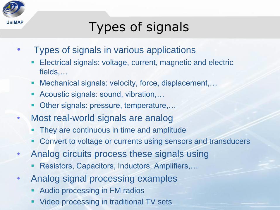
Types of signals

• Types of signals in various applications

Electrical signals: voltage, current, magnetic and electric

fields,…

Mechanical signals: velocity, force, displacement,…

Acoustic signals: sound, vibration,…

Other signals: pressure, temperature,…

• Most real-world signals are analog

They are continuous in time and amplitude

Convert to voltage or currents using sensors and transducers

• Analog circuits process these signals using

Resistors, Capacitors, Inductors, Amplifiers,…

• Analog signal processing examples

Audio processing in FM radios

Video processing in traditional TV sets

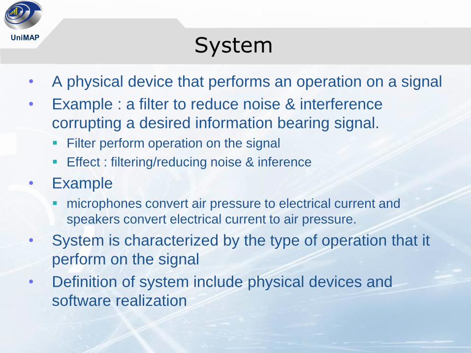
System

• A physical device that performs an operation on a signal

• Example : a filter to reduce noise & interference

corrupting a desired information bearing signal.

Filter perform operation on the signal

Effect : filtering/reducing noise & inference

• Example

microphones convert air pressure to electrical current and

speakers convert electrical current to air pressure.

• System is characterized by the type of operation that it

perform on the signal

• Definition of system include physical devices and

software realization

Digital Signal

• Digital signal processing (DSP) is concerned with the

digital representation of signals and the use of digital

processors to analyse, modify, or extract information

from signals.

• Many signals in DSP are derived from analogue signals

which have been sampled at regular intervals and

converted into digital form.

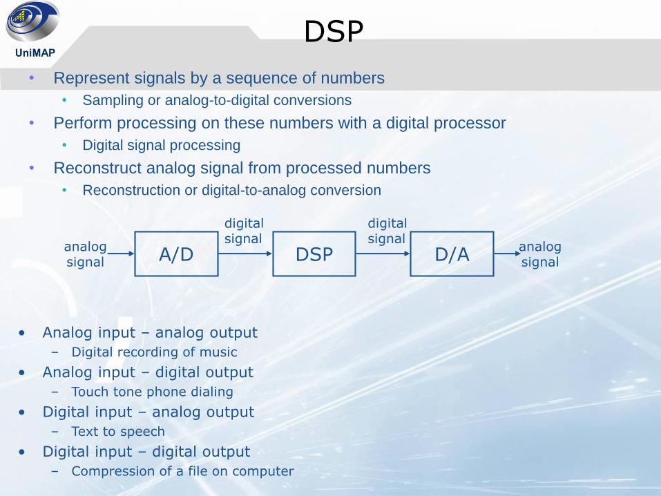
DSP

• Represent signals by a sequence of numbers

• Sampling or analog-to-digital conversions

• Perform processing on these numbers with a digital processor

• Digital signal processing

• Reconstruct analog signal from processed numbers

• Reconstruction or digital-to-analog conversion

A/D DSP D/Aanalogsignal

analogsignal

digital signal

digital signal

• Analog input – analog output

– Digital recording of music

• Analog input – digital output

– Touch tone phone dialing

• Digital input – analog output

– Text to speech

• Digital input – digital output

– Compression of a file on computer

Pros and Cons of Digital Signal Processing

• Pros

Accuracy can be controlled by choosing word length

Repeatable

Sensitivity to electrical noise is minimal

Dynamic range can be controlled using floating point numbers

Flexibility can be achieved with software implementations

Non-linear and time-varying operations are easier to implement

Digital storage is cheap

Digital information can be encrypted for security

Price/performance and reduced time-to-market

• Cons

Sampling causes loss of information

A/D and D/A requires mixed-signal hardware

Limited speed of processors

Quantization and round-off errors

Test ur understanding

Key operation in DSP

• Convolution

• Correlation

• Filtering

• Transformation

• Modulation

All basic DSP operations require only simple

arithmetic operations of multiply,

add/substract and shift to carry out.

Basic Operation

• Product (modulation) operation:

y[n]=x[n].w[n]

Modulator:

• An application is in forming a finite-length

sequence from an infinite-length sequence by

multiplying with a window sequence. This

process is usually called windowing

Basic Operations

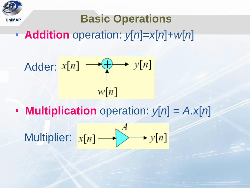
• Addition operation: y[n]=x[n]+w[n]

Adder:

• Multiplication operation: y[n] = A.x[n]

Multiplier:

Basic Operations

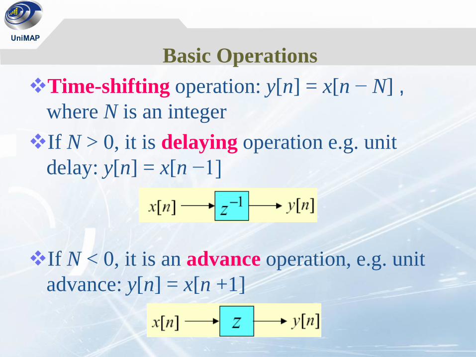
Time-shifting operation: y[n] = x[n − N] ,

where N is an integer

If N > 0, it is delaying operation e.g. unit

delay: y[n] = x[n −1]

If N < 0, it is an advance operation, e.g. unit

advance: y[n] = x[n +1]

Basic Operations

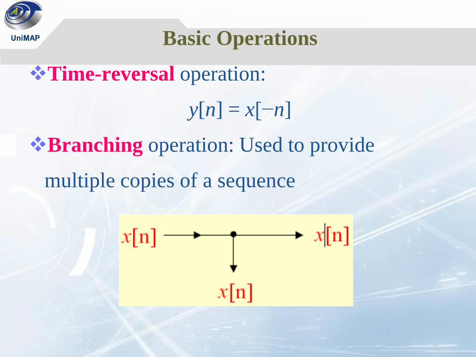
Time-reversal operation:

y[n] = x[−n]

Branching operation: Used to provide

multiple copies of a sequence

21

Basic Operations

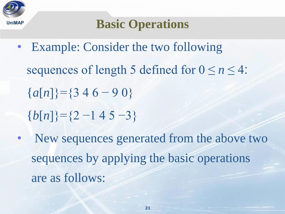
• Example: Consider the two following

sequences of length 5 defined for 0 ≤ n ≤ 4:

{a[n]}={3 4 6 − 9 0}

{b[n]}={2 −1 4 5 −3}

• New sequences generated from the above two

sequences by applying the basic operations

are as follows:

22

Basic Operations

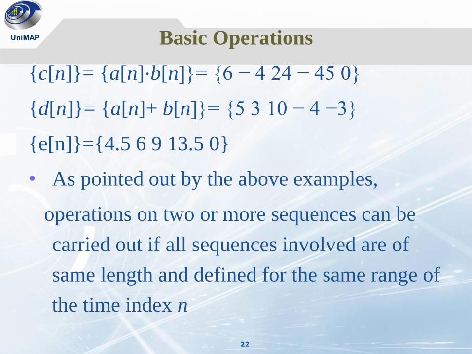
{c[n]}= {a[n]⋅b[n]}= {6 − 4 24 − 45 0}

{d[n]}= {a[n]+ b[n]}= {5 3 10 − 4 −3}

{e[n]}={4.5 6 9 13.5 0}

• As pointed out by the above examples,

operations on two or more sequences can be

carried out if all sequences involved are of

same length and defined for the same range of

the time index n

23

Basic Operations

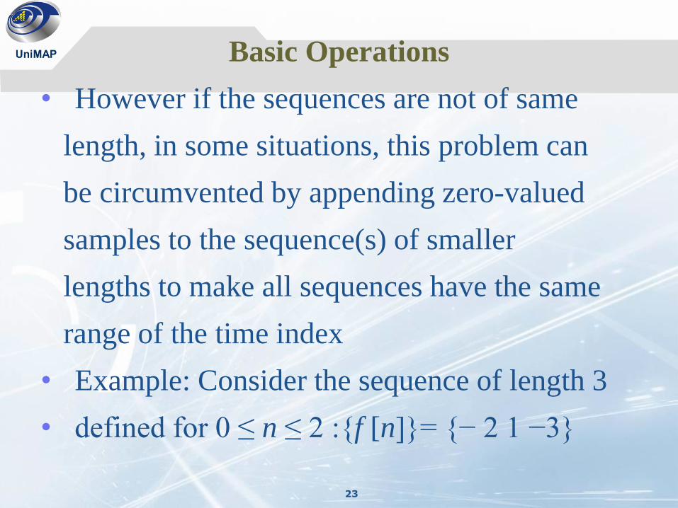
• However if the sequences are not of same

length, in some situations, this problem can

be circumvented by appending zero-valued

samples to the sequence(s) of smaller

lengths to make all sequences have the same

range of the time index

• Example: Consider the sequence of length 3

• defined for 0 ≤ n ≤ 2 :{f [n]}= {− 2 1 −3}

24

Basic Operations

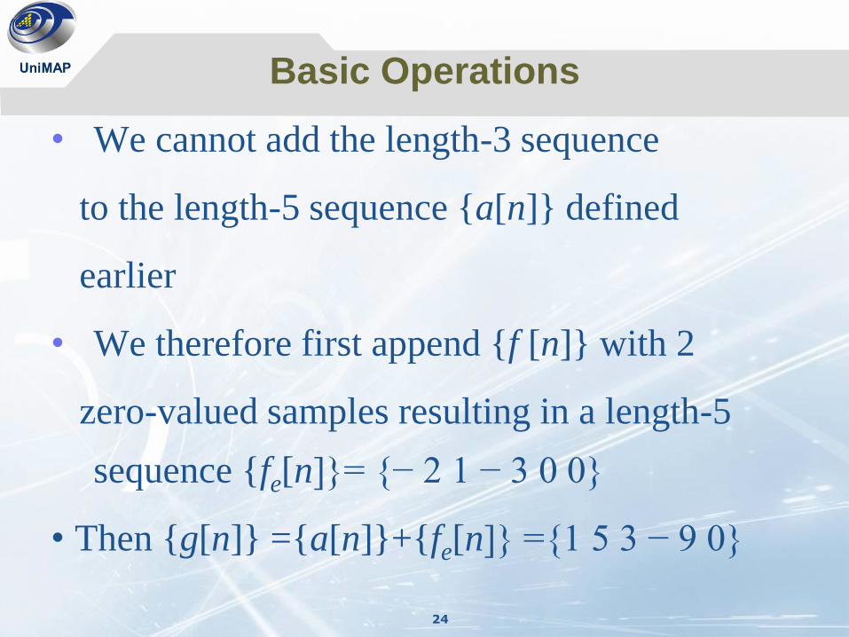
• We cannot add the length-3 sequence

to the length-5 sequence {a[n]} defined

earlier

• We therefore first append {f [n]} with 2

zero-valued samples resulting in a length-5

sequence {fe[n]}= {− 2 1 − 3 0 0}

• Then {g[n]} ={a[n]}+{fe[n]} ={1 5 3 − 9 0}

25

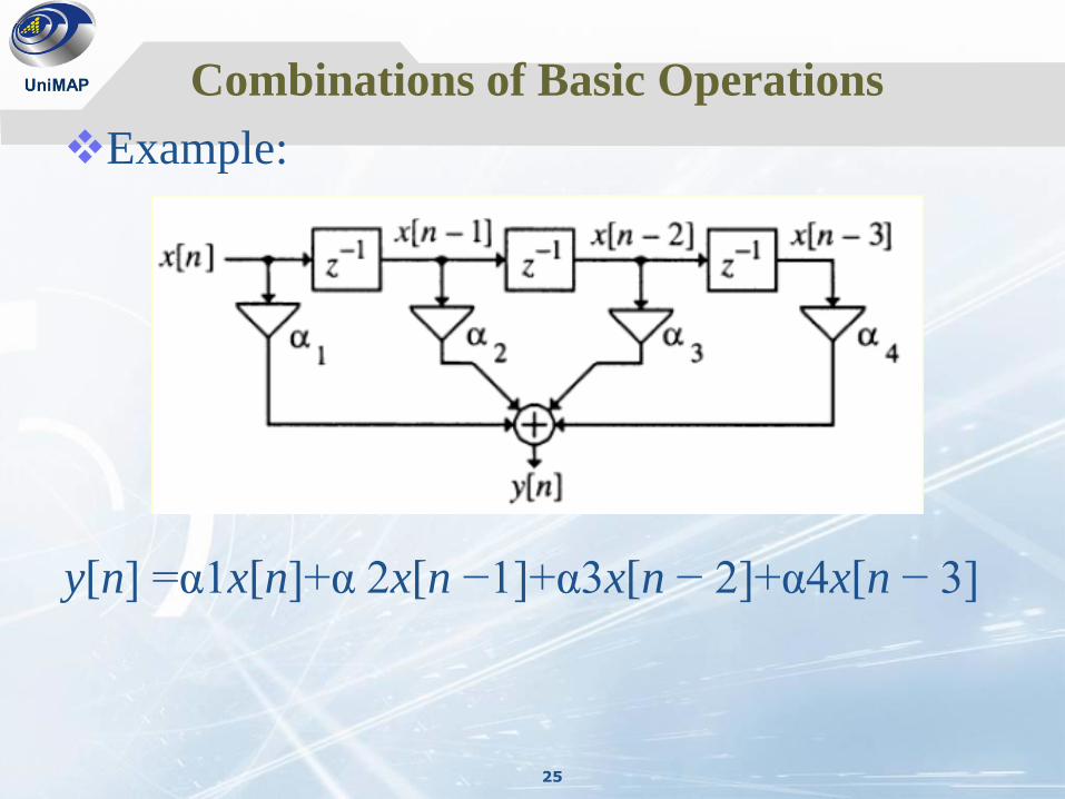
Combinations of Basic Operations

Example:

y[n] =α1x[n]+α 2x[n −1]+α3x[n − 2]+α4x[n − 3]

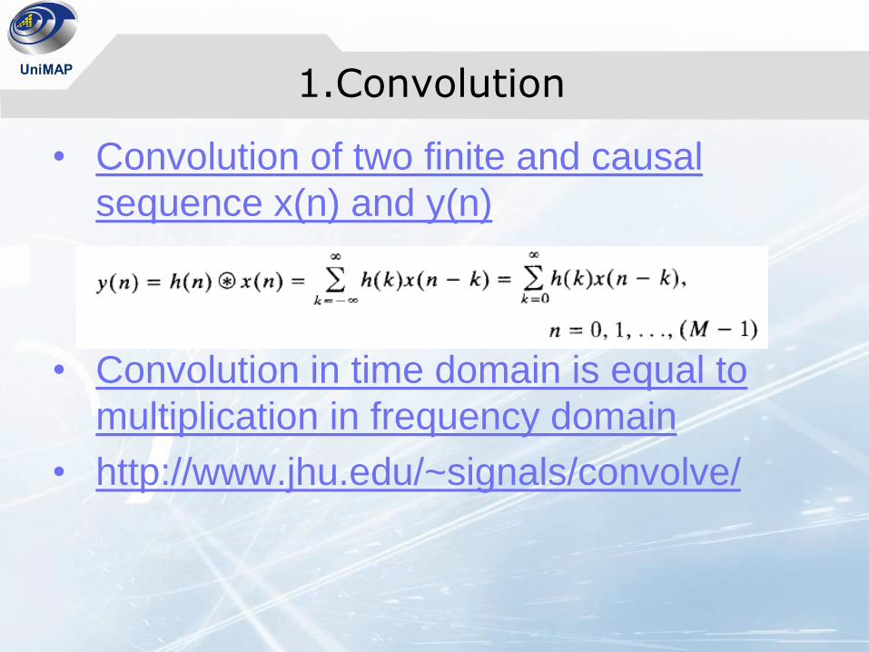
1.Convolution

• Convolution of two finite and causal

sequence x(n) and y(n)

• Convolution in time domain is equal to

multiplication in frequency domain

• http://www.jhu.edu/~signals/convolve/

2.Correlation

Auto correlation Involve only one signal and

provides information about the

structure of the signal and its

behaviour in the time domain.

Useful in identifying hidden

periodicities.

Cross correlation (CCF) Is a measure of similarities or

shared properties between two

signals

Example : Cross spectral

analysis, pattern matching,

delay measurement.

Cross correlation

of random signal

Delayed

noisy signal

Cross correlation

Delay between 2

signal

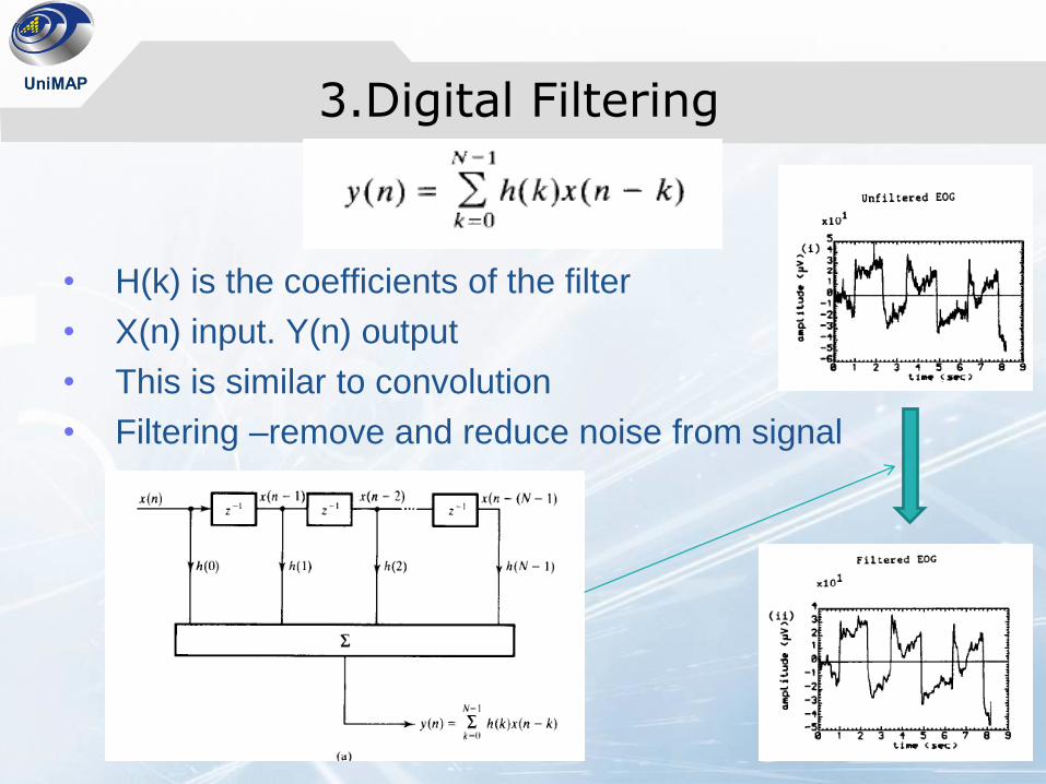
3.Digital Filtering

• H(k) is the coefficients of the filter

• X(n) input. Y(n) output

• This is similar to convolution

• Filtering –remove and reduce noise from signal

Operation

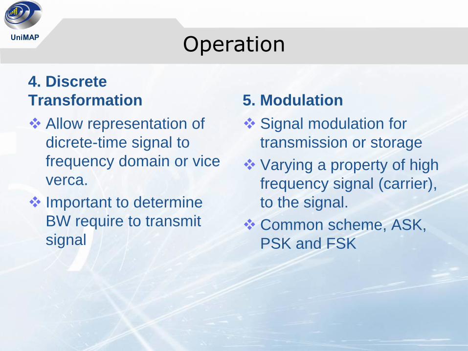
4. Discrete

Transformation

Allow representation of

dicrete-time signal to

frequency domain or vice

verca.

Important to determine

BW require to transmit

signal

5. Modulation

Signal modulation for

transmission or storage

Varying a property of high

frequency signal (carrier),

to the signal.

Common scheme, ASK,

PSK and FSK

UniMAP

Sampling

Part 2

Periodic (Uniform) Sampling

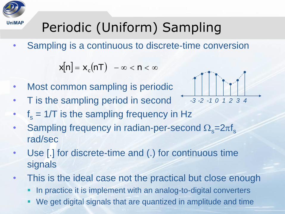
• Sampling is a continuous to discrete-time conversion

• Most common sampling is periodic

• T is the sampling period in second

• fs = 1/T is the sampling frequency in Hz

• Sampling frequency in radian-per-second s=2fs

rad/sec

• Use [.] for discrete-time and (.) for continuous time

signals

• This is the ideal case not the practical but close enough

In practice it is implement with an analog-to-digital converters

We get digital signals that are quantized in amplitude and time

nnTxnx c

-3 -2 2 3 4-1 10

Periodic Sampling

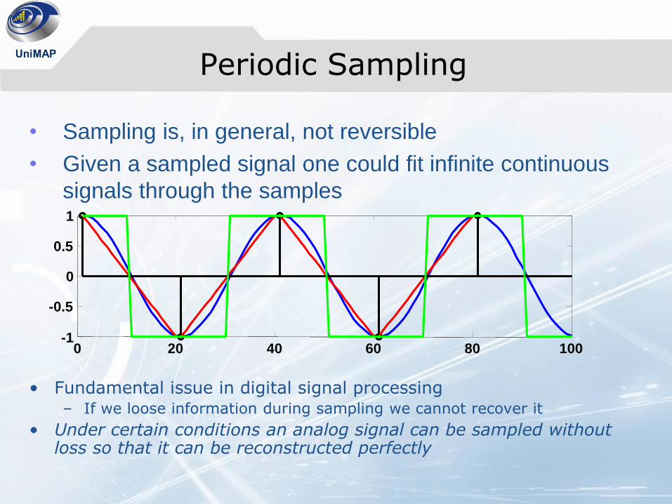
• Sampling is, in general, not reversible

• Given a sampled signal one could fit infinite continuous

signals through the samples

0-1

20 40 60 80 100

-0.5

0

0.5

1

• Fundamental issue in digital signal processing– If we loose information during sampling we cannot recover it

• Under certain conditions an analog signal can be sampled without loss so that it can be reconstructed perfectly

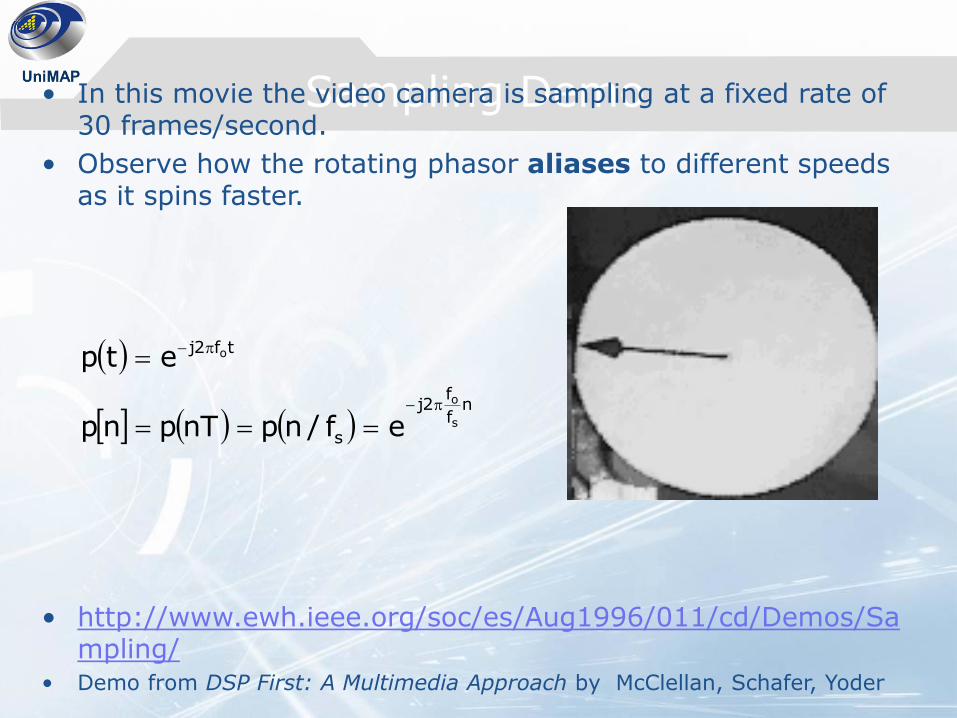
Sampling Demo• In this movie the video camera is sampling at a fixed rate of 30 frames/second.

• Observe how the rotating phasor aliases to different speeds as it spins faster.

• http://www.ewh.ieee.org/soc/es/Aug1996/011/cd/Demos/Sampling/

• Demo from DSP First: A Multimedia Approach by McClellan, Schafer, Yoder

n

f

f2j

s

tf2j

s

o

o

ef/npnTpnp

etp

Aliasing effect

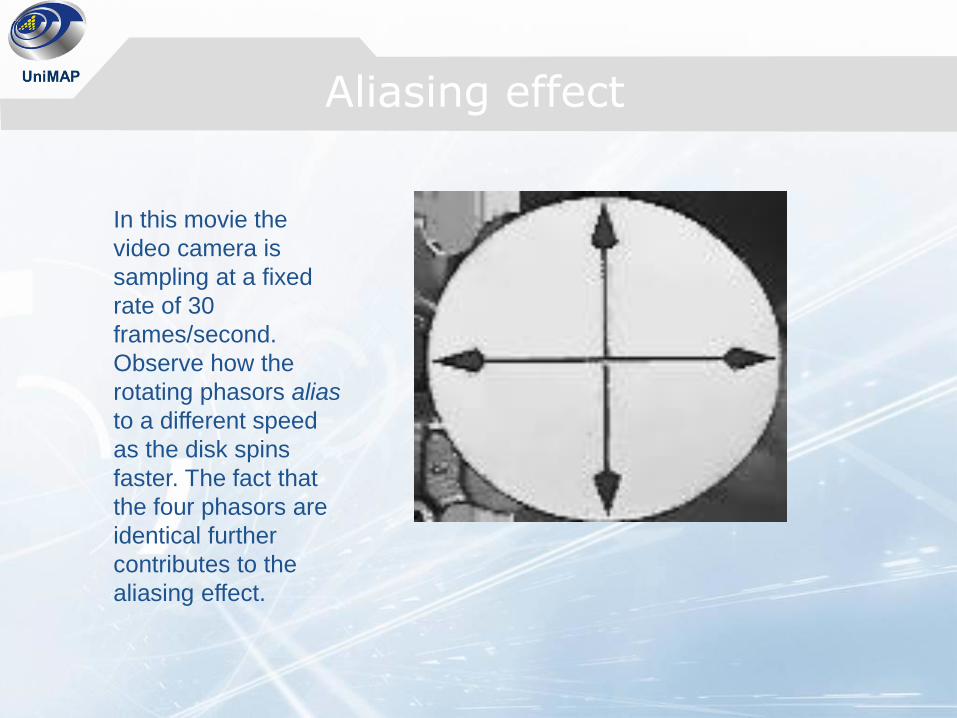
In this movie the

video camera is

sampling at a fixed

rate of 30

frames/second.

Observe how the

rotating phasors alias

to a different speed

as the disk spins

faster. The fact that

the four phasors are

identical further

contributes to the

aliasing effect.

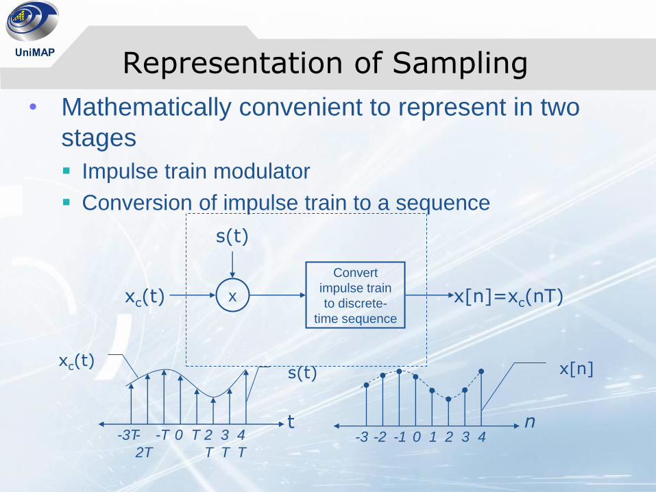
Representation of Sampling

• Mathematically convenient to represent in two

stages

Impulse train modulator

Conversion of impulse train to a sequence

Convert

impulse train

to discrete-

time sequence

xc(t) x[n]=xc(nT)x

s(t)

-3T-

2T

2

T

3

T

4

T

-T T0

s(t)xc(t)

t

x[n]

-3 -2 2 3 4-1 10n

36

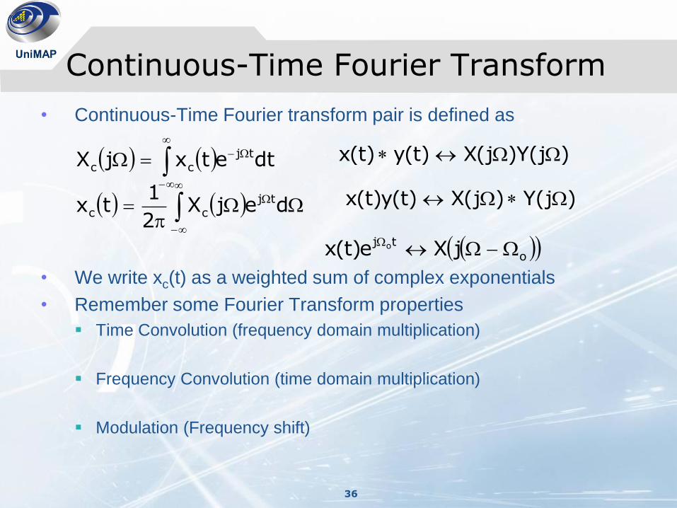
Continuous-Time Fourier Transform

• Continuous-Time Fourier transform pair is defined as

• We write xc(t) as a weighted sum of complex exponentials

• Remember some Fourier Transform properties

Time Convolution (frequency domain multiplication)

Frequency Convolution (time domain multiplication)

Modulation (Frequency shift)

dtetxjX tjcc

dejX2

1tx tj

cc

)j(Y)j(X)t(y)t(x

)j(Y)j(X)t(y)t(x

o

tj jXe)t(x o

351M Digital Signal Processing37

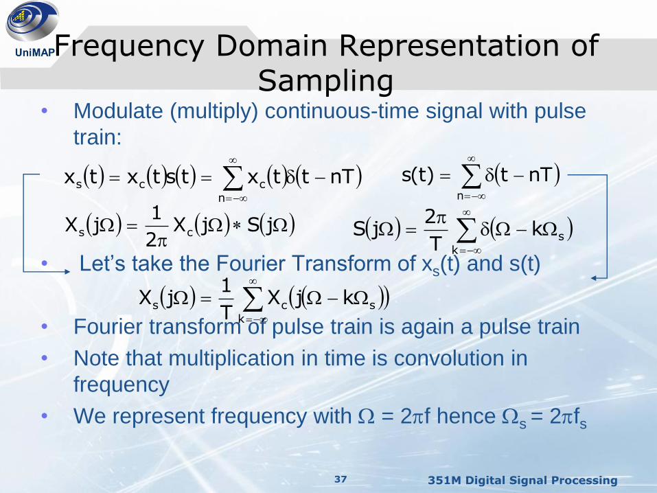
Frequency Domain Representation of Sampling

• Modulate (multiply) continuous-time signal with pulse

train:

• Let’s take the Fourier Transform of xs(t) and s(t)

• Fourier transform of pulse train is again a pulse train

• Note that multiplication in time is convolution in

frequency

• We represent frequency with = 2f hence s = 2fs

n

nTt)t(s

n

ccs nTttxtstxtx

k

skT

2jS

jSjX

2

1jX cs

k

scs kjXT

1jX

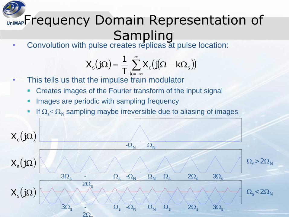
Frequency Domain Representation of Sampling

• Convolution with pulse creates replicas at pulse location:

• This tells us that the impulse train modulator

Creates images of the Fourier transform of the input signal

Images are periodic with sampling frequency

If s< N sampling maybe irreversible due to aliasing of images

k

scs kjXT

1jX

jXc

jXs

jXs

N-N

N-N s 2s 3s-

2s

s3s

N-N s 2s 3s-

2s

s3s

s<2N

s>2N

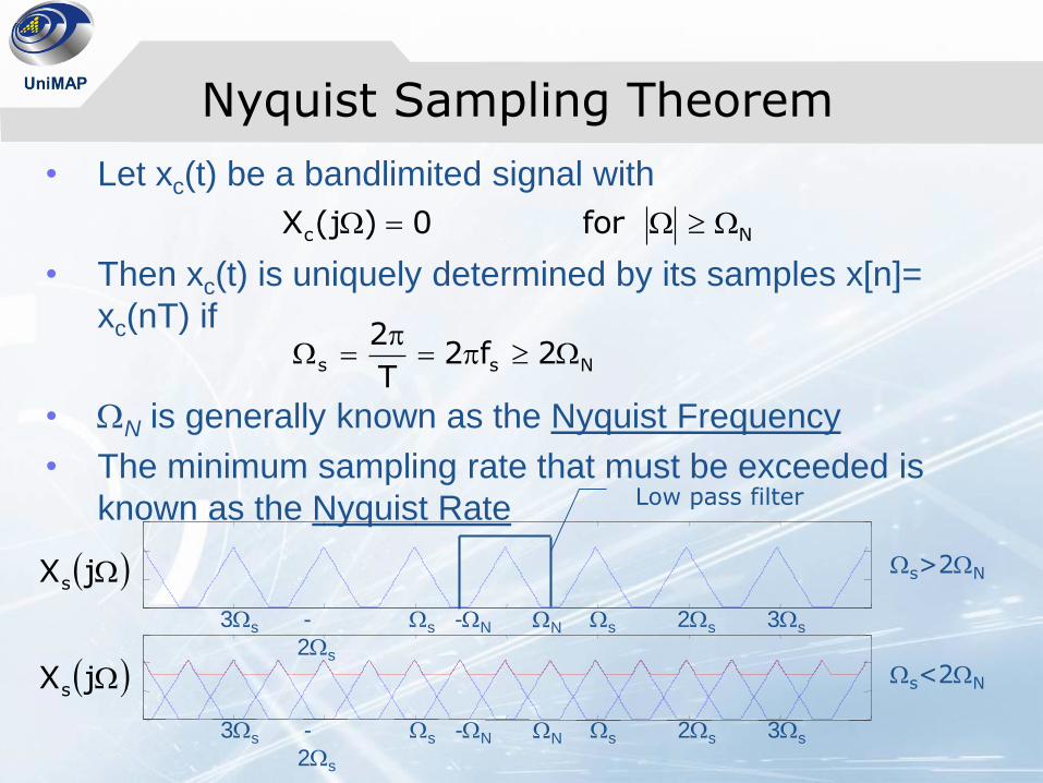
Nyquist Sampling Theorem

• Let xc(t) be a bandlimited signal with

• Then xc(t) is uniquely determined by its samples x[n]=

xc(nT) if

• N is generally known as the Nyquist Frequency

• The minimum sampling rate that must be exceeded is

known as the Nyquist Rate

Nc for 0)j(X

Nss 2f2T

2

jXs

jXs

N-N s 2s 3s-

2s

s3s

N-N s 2s 3s-

2s

s3s

s<2N

s>2N

Low pass filter

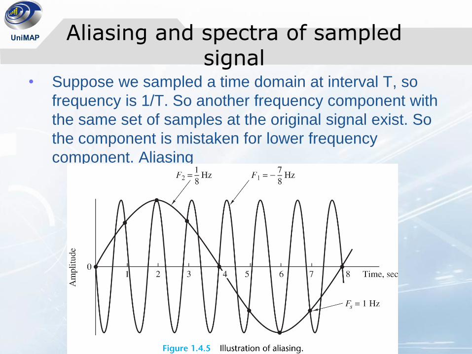
Aliasing and spectra of sampled signal

• Suppose we sampled a time domain at interval T, so

frequency is 1/T. So another frequency component with

the same set of samples at the original signal exist. So

the component is mistaken for lower frequency

component. Aliasing

Demo

Aliasing demo

http://www.ami.ac.uk/courses/topics/0020_aliasdemo/ind

ex.html

Sample Mania

http://www.jhu.edu/~signals/sampling/index.html

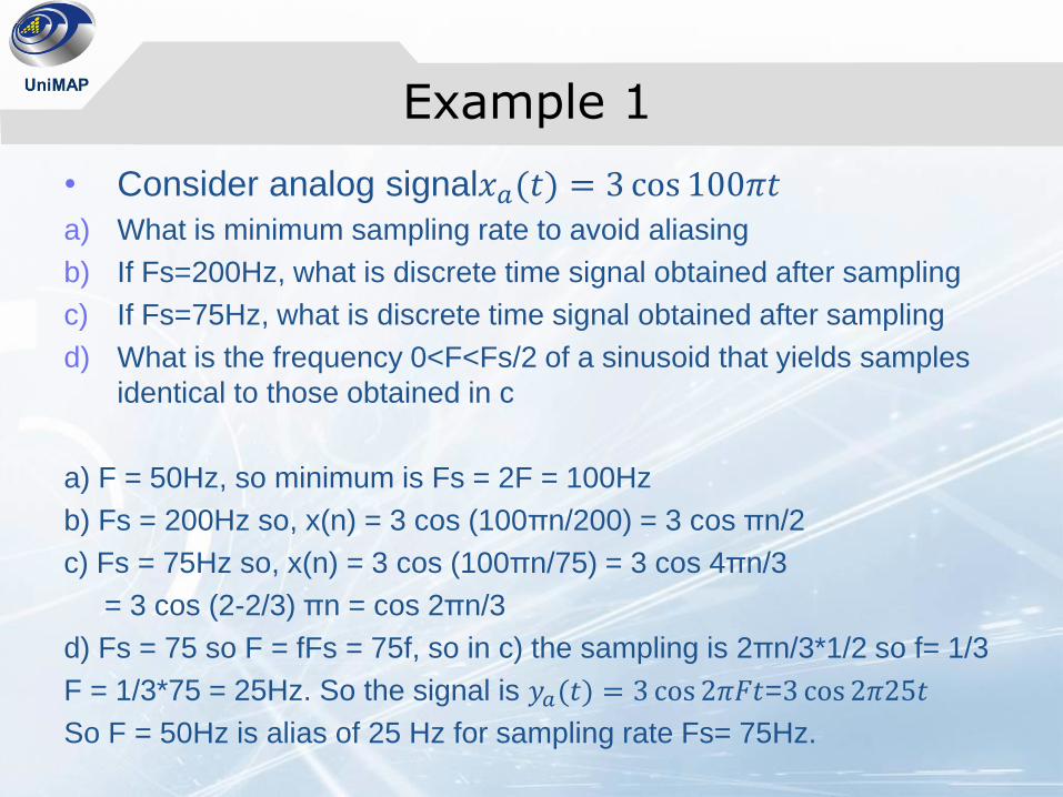
Example 1

• Consider analog signal𝑥𝑎(𝑡) = 3 cos 100𝜋𝑡a) What is minimum sampling rate to avoid aliasing

b) If Fs=200Hz, what is discrete time signal obtained after sampling

c) If Fs=75Hz, what is discrete time signal obtained after sampling

d) What is the frequency 0<F<Fs/2 of a sinusoid that yields samples

identical to those obtained in c

a) F = 50Hz, so minimum is Fs = 2F = 100Hz

b) Fs = 200Hz so, x(n) = 3 cos (100πn/200) = 3 cos πn/2

c) Fs = 75Hz so, x(n) = 3 cos (100πn/75) = 3 cos 4πn/3

= 3 cos (2-2/3) πn = cos 2πn/3

d) Fs = 75 so F = fFs = 75f, so in c) the sampling is 2πn/3*1/2 so f= 1/3

F = 1/3*75 = 25Hz. So the signal is 𝑦𝑎(𝑡) = 3 cos 2𝜋𝐹𝑡=3 cos 2𝜋25𝑡

So F = 50Hz is alias of 25 Hz for sampling rate Fs= 75Hz.

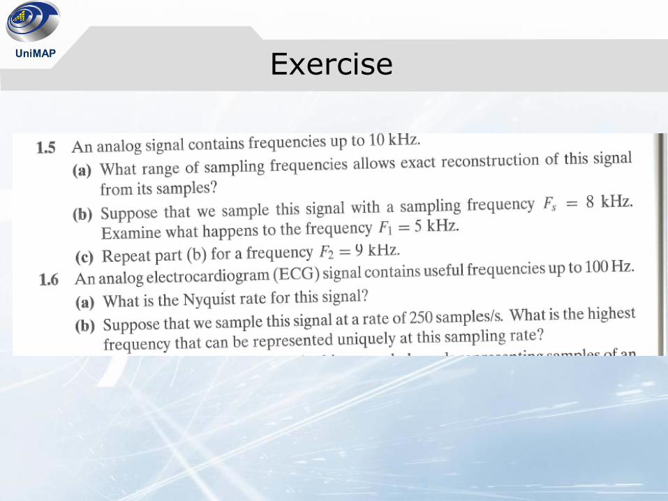
Exercise

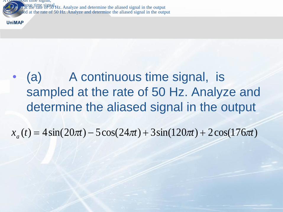
• (a) A continuous time signal, is

sampled at the rate of 50 Hz. Analyze and

determine the aliased signal in the output

A continuous time signal,

is sampled at the rate of 50 Hz. Analyze and determine the aliased signal in the outputA continuous time signal,

is sampled at the rate of 50 Hz. Analyze and determine the aliased signal in the output

)176cos(2)120sin(3)24cos(5)20sin(4)( tttttxa