challenging the versatility of the tesla turbine: working fluid variations and turbine ... · ·...
TRANSCRIPT
Challenging the Versatility of the Tesla Turbine:
Working Fluid Variations and Turbine Performance
by
Aaron Peshlakai
A Thesis Presented in Partial Fulfillment
of the Requirements for the Degree
Master of Science
Approved November 2012 by the
Graduate Supervisory Committee:
Patrick Phelan, Chair
Liping Wang
Steven Trimble
ARIZONA STATE UNIVERSITY
December 2012

i
ABSTRACT
Tesla turbo-machinery offers a robust, easily manufactured, extremely
versatile prime mover with inherent capabilities making it perhaps the best, if not
the only, solution for certain niche applications. The goal of this thesis is not to
optimize the performance of the Tesla turbine, but to compare its performance
with various working fluids.
Theoretical and experimental analyses of a turbine-generator assembly
utilizing compressed air, saturated steam and water as the working fluids were
performed and are presented in this work. A brief background and explanation of
the technology is provided along with potential applications. A theoretical
thermodynamic analysis is outlined, resulting in turbine and rotor efficiencies,
power outputs and Reynolds numbers calculated for the turbine for various
combinations of working fluids and inlet nozzles.
The results indicate the turbine is capable of achieving a turbine efficiency
of 31.17 ± 3.61% and an estimated rotor efficiency 95 ± 9.32%. These
efficiencies are promising considering the numerous losses still present in the
current design.
Calculation of the Reynolds number provided some capability to
determine the flow behavior and how that behavior impacts the performance and
efficiency of the Tesla turbine. It was determined that turbulence in the flow is
essential to achieving high power outputs and high efficiency. Although the
efficiency, after peaking, begins to slightly taper off as the flow becomes
increasingly turbulent, the power output maintains a steady linear increase.

ii
Without my girls I wouldn’t have high aspirations.
Without my wife I couldn’t achieve them.

iii
ACKNOWLEDGMENTS
The author would like to acknowledge several individuals who provided
guidance, support and advice throughout this work. Dr. Patrick Phelan provided
valuable insight into the overall design and modeling of the turbine and
accompanying power system. Dr. Steven Trimble introduced the necessary tools
to acquire the engineering business acumen for commercial advancement of this
work. Dr. Kenneth Huebner gave a group of naïve underclassman the chance to
stretch their minds and push their limits. Dr. Liping Wang stepped in to fill a vital
role with little hesitation and even less of a heads up. John Sherbeck freely shared
his experience, intuition and machinery making vast improvements to the design
and performance of the turbine genset. Jesse DeWitt took on a difficult task that
will advance this work greatly in the years ahead. Anita Grierson provided
constant advice and encouragement. Dimitris Papachristoforou and John Song
saw the potential that others could not and acted on it. Lennix Peshlakai and ASU
Innovation Challenge provided the financial support to make this idea come to
life. Thanks to all.

iv
TABLE OF CONTENTS
Page
LIST OF TABLES ..................................................................................................... vii
LIST OF FIGURES .................................................................................................. viii
NOMENCLATURE .................................................................................................... x
CHAPTER
1 THE TESLA TURBINE ....................................................................... 1
1.1 Background ................................................................................. 1
1.2 How it works ............................................................................... 3
1.3 Potential Applications................................................................. 5
1.4 Literature Review ....................................................................... 7
1.5 Research Questions..................................................................... 8
2 THEORETICAL PERFORMANCE: THERMODYNAMICS ......... 10
2.1 General Assumptions ................................................................ 10
2.1.1 Compressed Air Assumptions ......................................... 10
2.1.2 Steam Assumptions ......................................................... 10
2.1.3 Water Assumptions ......................................................... 11
2.2 Known Variables ...................................................................... 11
2.2.1 Known Compressed Air Variables ................................. 11
2.2.2 Known Steam Variables .................................................. 11
2.2.3 Known Water Variables .................................................. 12
2.3 Fluid Flow Analysis State Points ............................................. 12
2.4 Air Flow Analysis ..................................................................... 13

v
CHAPTER Page
2.5 Steam Flow Analysis ................................................................ 14
2.6 Water Flow Analysis ................................................................ 15
2.7 Mechanical Energy Analysis for Air and Steam ..................... 16
2.8 Mechanical Energy Analysis for Water ................................... 16
2.9 Heat Loss Analysis ................................................................... 16
2.10 Nozzle Losses ......................................................................... 18
2.11 Rotor Efficiency...................................................................... 19
2.12 Turbine Efficiency .................................................................. 19
2.13 Reynolds Number ................................................................... 20
2.14 Uncertainty .............................................................................. 22
3 EXPERIMENTAL SETUP .................................................................. 23
3.1 Rotor Specifications ................................................................. 23
3.2 Nozzles ...................................................................................... 24
3.3 Turbine GenSet ......................................................................... 25
3.4 Compressed Air Setup .............................................................. 26
3.5 Steam Setup .............................................................................. 27
3.6 Pressurized Water Setup ........................................................... 28
4 RESULTS AND DISCUSSION .......................................................... 29
4.1 Rotor Efficiency ........................................................................ 29
4.2 Turbine Efficiency .................................................................... 32
4.3 Power Performance................................................................... 33
4.4 Reynolds Number and Flow Characterisitcs ........................... 35
vi
CHAPTER Page
4.5 Steam Testing Complications................................................... 37
4.6 Projected Saturated Steam Requirements ................................ 38
5 FUTURE WORK AND CONCLUSIONS ......................................... 40
5.1 Future Turbine Work ............................................................... 40
5.2 Future Steam Generator Work ................................................. 42
5.3 Primary Application: Future Solar Power Unit Work ............. 42
5.3 Future Solar Power Unit Work ................................................ 42
5.4 Other Potential Applications to Investigate ............................. 43
5.5 Future Analysis ......................................................................... 43
5.6 Conclusions ............................................................................... 44
REFERENCES ........................................................................................................ 46
APPENDIX
A UNCERTIANTIES FOR MEASUREMENT DEVICES ............... 48

vii
LIST OF TABLES
Table Page
1. Peak Rotor Efficiencies ......................................................................... 31
2. Maximum Power Outputs Achieved .................................................. 34
3. Qualitative Comparison of Air and Steam .......................................... 38
4. Projected Steam Requirements for Nozzle 1: Max Power ................ 39
5. Projected Steam Requirements for Nozzle 2: Max Power ................. 39
6. Uncertainties for Measurement Devices ............................................ 49

viii
LIST OF FIGURES
Figure Page
1. Original Schematic of the Tesla Turbine ............................................... 1
2. Tesla Turbine Complete Assembly ....................................................... 3
3. Tesla Turbine Rotor, Disks and Shaft ................................................... 3
4. Schematic of Fluid Flow through the Tesla Turbine ............................ 4
5. Original Schematic of a Tesla Pump ..................................................... 5
6. Efficiency vs Power Output for Tesla and Bladed Turbines ................ 5
7. Schematic Identifying State Points ...................................................... 12
8. Rotor Schematic Discretized Disk Bands ........................................... 21
9. Rotor Schematic with Relevant Dimensions ....................................... 23
10. Nozzle 1 .............................................................................................. 24
11. Nozzle 2 .............................................................................................. 24
12. Turbine GenSet ................................................................................... 25
13. Compressed Air Setup ........................................................................ 26
14. Steam Setup ......................................................................................... 27
15. Pressurized Water Setup ..................................................................... 28
16. Rotor Efficiency vs Mass Flow Rate – Nozzle 1 Air ......................... 29
17. Rotor Efficiency vs Mass Flow Rate – Nozzle 2 Air ......................... 30
18. Turbine Efficiency vs Mass Flow Rate – Nozzle 1 Air ..................... 32
19. Turbine Efficiency vs Mass Flow Rate – Nozzle 1 Air ..................... 33
20. Turbine Power vs Mass Flow Rate – Nozzle 1 Air............................ 33
21. Turbine Power vs Mass Flow Rate – Nozzle 2 Air............................ 34

ix
Figure Page
22. Turbine Efficiency vs Reynolds Number – Nozzle 1 Air ................. 35
23. Turbine Efficiency vs Reynolds Number – Nozzle 2 Air .................. 35

x
LIST OF SYMBOLS
Symbol Definition [Units]
A ....................................................................................................... Area [m2]
b .................................................................................... Disk gap spacing [m]
cp ................................................................................. Specific heat [kJ/kg·K]
D ................................................................................................. Diameter [m]
h ............................................................................................ Enthalpy [kJ/kg]
h’ ..................................... Enthalpy at equilibrium with surroundings [kJ/kg]
hL ............................................................................................... Head Loss [m]
ht ............................................................................. Heat Transfer Coefficient
k .......................................................................................... Specific heat ratio
KL ............................................................................................. Loss coefficient
L ........................................................................................... Flow Length [m]
....................................................................................... Mass flow rate [g/s]
Nu ............................................................................................. Nusselt Number
Pamb ................................................................................ Ambient pressure [kPa]
P* ....................................................................... Critical nozzle pressure [kPa]
Q .......................................................................... Volumetric flow rate [m3/s]
q .................................. Individual surface heat transfer to surroundings [W]
..................................................... Total Heat transfer to surroundings [W]
R ............................................................................. Gas constant [kJ/kmol·K]
Re ......................................................................................... Reynolds Number
Ra .......................................................................................... Rayleigh Number

xi
Symbol Definition [Units]
s ......................................................................................... Entropy [kJ/kg·K]
s’ ................................... Entropy at equilibrium with surroundings [kJ/kg·K]
...................................................................... Entropy generation [kJ/kg·K]
T ................................................................. Temperature of surroundings [K]
T* .................................................................... Critical nozzle temperature [K]
Tf .................................................................................... Film temperature [K]
TK ................................................................................ Surface temperature [K]
V ........................................................................ Working fluid velocity [m/s]
.............................................................................. Turbine work output [W]
..........................................................................Mechanical fluid work [W]
ηRotor ................................................................... Mechanical efficiency of rotor
ρ ............................................................................................. Density [kg/m3]
ρ* ..................................................................... Critical nozzle density [kg/m3]
z .............................................. Perpendicular distance from disk surface [m]
Subscript Definition
Inlet ...................................................................... Prior to entering nozzle shaft
rR ..................................................................... Dependent on radial location
0 ..................................................................................... Stagnation condition
1 ......................................................................................... Inside nozzle shaft
2 .............................................................................. Nozzle outlet, Rotor inlet
3 ...................................................................................... Rotor/Turbine outlet

1
CHAPTER 1
THE TESLA TURBINE
1.1 Background
Patented in 1913 [1], the Tesla turbine, also referred to as a flat-plate
turbine or boundary layer turbine, is a fairly simple device with few moving parts
and was invented by Nikola Tesla. The turbine consists of a series of flat, round
plates fixed to a shaft housed within a plenum chamber. Work is produced when
the working fluid is introduced tangentially at the outer edge of the plates and
exits the turbine at exhaust ports located near the center of the disks. A schematic
provided by Tesla as part of his U.S. patent for the turbine is shown in Figure 1.
When work is applied to the shaft, the device then acts as a pump or compressor
pushing fluid from the center to the outer edges of the disks.
Figure 1 Original schematic of the Tesla turbine [1].
The Tesla turbine was invented in order to produce power from fluid
motion. Among the many claims made by Tesla regarding his turbine, was its

2
high power to weight ratio, a common metric used at the time to evaluate a
turbine’s usefulness. In fact, Tesla claimed to have invented a steam Tesla turbine
capable of producing 200 hp with only an 18-inch rotor [2]. This turbine was
advertised as a “powerful engine” that “could be covered by a hat” [3]
Tesla, however, was never able to achieve industrial applications of his
device due to the relatively low turbine efficiency compared to the traditional
bladed turbines still in use today [4]. The primary reason for this low efficiency
has been attributed to losses at the inlet and nozzle [4,5]. Other reasons for the
low efficiency are losses in the bearings, viscous losses in the end walls and
dissipative losses in the plenum chamber; all of these losses reportedly reducing
the turbine efficiency by up to 15% [6]. The turbine efficiencies reported in these
referenced texts should not be confused with the rotor efficiency reported in this
paper. The reported turbine efficiencies include the nozzle and the entire turbine
in the control volume. The rotor efficiency outline in this work does not include
the nozzle.
Another major benefit of the Tesla turbine lies in its simple design and
fabrication requirements. It is relatively inexpensive to manufacture due to its
design simplicity when compared to costs associated with traditional bladed
turbines. In fact, an adequate Tesla turbine can be made using basic tools that can
be found in any modest machine shop.
In recent years, the use of Tesla’s design has been gaining some ground
for use where conventional turbines are inadequate – highly viscous fluids, fluids
containing abrasive particles, and two-phase fluids [4].

3
1.2 How it works
An attractive feature of the Tesla turbine from a manufacturing standpoint
is its simplicity. The entire turbine assembly, taken apart for ease of explanation,
is shown in Figure 2.
Figure 2 Entire Tesla turbine assembly showing the rotor blades, housing, inlet
nozzle and exhaust. Ruler (cm) added for approximate size scale.
The Tesla turbine design is distinguished by its use of flat, co-rotating
disks equally spaced and fixed along the rotor shaft which can be seen in Figure 3.
The rotor is housed by a metal casing which contains the inlet nozzle as well as
the exhaust ports.
When a fluid is introduced through the
nozzle, the fluid velocity is significantly
increased and is ejected tangentially towards the
outer edge of the disks. The viscosity of the
high-speed fluid and the no-slip condition along Figure 3 Tesla turbine rotor
with disks fixed to a shaft.

4
the disk surfaces results in momentum exchange from the fluid to the disks,
producing shaft torque and power output. As this exchange occurs, the fluid
spirals towards the center of the shaft where it is exhausted through ports located
near the center of the disks. A schematic of Tesla turbine flow theory is shown in
Figure 4.
Figure 4 Schematic of fluid flow through the Tesla turbine. All major turbine
components are shown and the actual rotor-housing clearance given.
As can be seen in Figure 4, there is nothing complicated about the way a
Tesla turbine works. The fact that the fluid flows parallel to the turbine disks
gives this design a distinct advantage over traditional bladed turbine; abrasive
particulates or even water droplets can be present in the working fluid without
risking direct impacts which could cause additional wear and damage to the disks.
Its ability to utilize a variety of fluids without damaging the blades and its
extremely low manufacturing cost warrant a renewed interest in the design.

5
When shaft power is supplied to
the rotor, the Tesla device can then be
used as a pump or a compressor [7]. The
process is simply the reverse of the turbine
explanation given above, with the fluid
flow from the center outward. Figure 5 is
the schematic provided by Tesla to explain
his design for a Tesla style pump or
compressor as part of an original patent.
1.3 Potential Applications
There has been some use of Tesla’s
design, whether as a turbine, compressor,
or pump; however, it hasn’t had many applications until recently due to its
relatively low efficiency compared to traditional turbines. It is common opinion
that bladed turbines are unbeatable at high power outputs; however at lower
outputs, bladeless turbines are superior [8]. The trend of efficiency vs. maximum
power output for both types of
turbines can be seen in Figure 6.
The performance and
efficiency of the rotor is dependent
on a few different variables: shaft
speed, disk inner and outer Figure 6 Efficiency vs Power output for
both Tesla and bladed turbines [8].
Figure 5 Original schematic of a
Tesla pump [7]
6
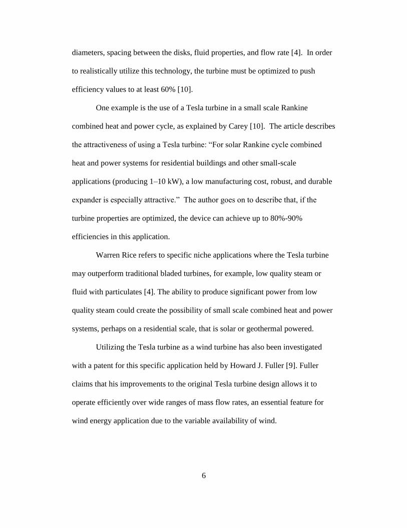
diameters, spacing between the disks, fluid properties, and flow rate [4]. In order
to realistically utilize this technology, the turbine must be optimized to push
efficiency values to at least 60% [10].
One example is the use of a Tesla turbine in a small scale Rankine
combined heat and power cycle, as explained by Carey [10]. The article describes
the attractiveness of using a Tesla turbine: “For solar Rankine cycle combined
heat and power systems for residential buildings and other small-scale
applications (producing 1–10 kW), a low manufacturing cost, robust, and durable
expander is especially attractive.” The author goes on to describe that, if the
turbine properties are optimized, the device can achieve up to 80%-90%
efficiencies in this application.
Warren Rice refers to specific niche applications where the Tesla turbine
may outperform traditional bladed turbines, for example, low quality steam or
fluid with particulates [4]. The ability to produce significant power from low
quality steam could create the possibility of small scale combined heat and power
systems, perhaps on a residential scale, that is solar or geothermal powered.
Utilizing the Tesla turbine as a wind turbine has also been investigated
with a patent for this specific application held by Howard J. Fuller [9]. Fuller
claims that his improvements to the original Tesla turbine design allows it to
operate efficiently over wide ranges of mass flow rates, an essential feature for
wind energy application due to the variable availability of wind.
7
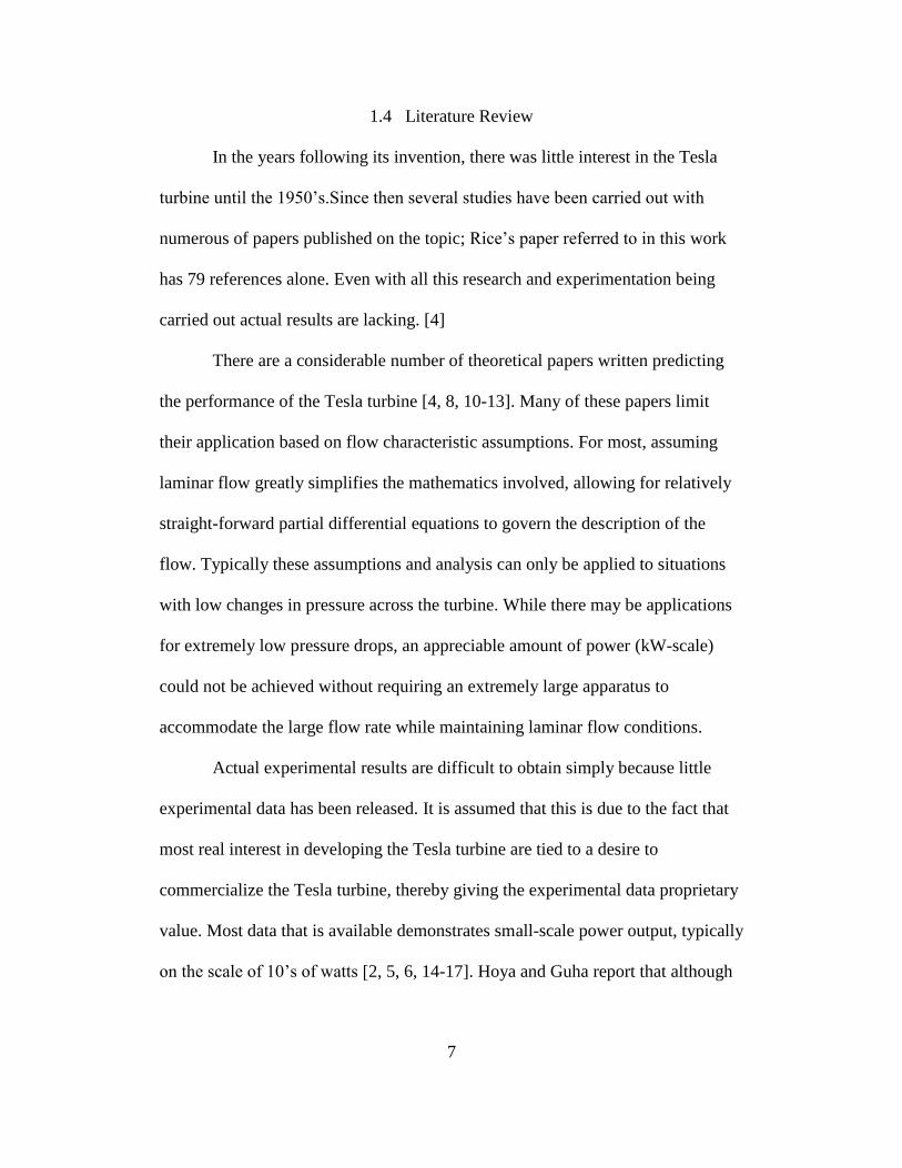
1.4 Literature Review
In the years following its invention, there was little interest in the Tesla
turbine until the 1950’s.Since then several studies have been carried out with
numerous of papers published on the topic; Rice’s paper referred to in this work
has 79 references alone. Even with all this research and experimentation being
carried out actual results are lacking. [4]
There are a considerable number of theoretical papers written predicting
the performance of the Tesla turbine [4, 8, 10-13]. Many of these papers limit
their application based on flow characteristic assumptions. For most, assuming
laminar flow greatly simplifies the mathematics involved, allowing for relatively
straight-forward partial differential equations to govern the description of the
flow. Typically these assumptions and analysis can only be applied to situations
with low changes in pressure across the turbine. While there may be applications
for extremely low pressure drops, an appreciable amount of power (kW-scale)
could not be achieved without requiring an extremely large apparatus to
accommodate the large flow rate while maintaining laminar flow conditions.
Actual experimental results are difficult to obtain simply because little
experimental data has been released. It is assumed that this is due to the fact that
most real interest in developing the Tesla turbine are tied to a desire to
commercialize the Tesla turbine, thereby giving the experimental data proprietary
value. Most data that is available demonstrates small-scale power output, typically
on the scale of 10’s of watts [2, 5, 6, 14-17]. Hoya and Guha report that although

8
Tesla reported power outputs of up to 200 hp, recent modern attempts have
yielded generally below 2 hp [2].
The vast majority of the experimental results published utilize air as the
working fluid. It is the author’s opinion that the best opportunity for the Tesla
turbine to gain significance would be related to steam or particulate laden fluid
applications. In particular, low quality steam power generation would be an ideal
situation. There is a definite lack of published experimental data where the
working fluid is steam of any quality.
1.5 Research Questions
This work seeks to challenge the versatility of a Tesla turbine, testing it
with a variety of working fluids under various conditions. Experiments were
performed using the same turbine and set of nozzles using air, water and steam as
the working fluid. No changes were made to the geometry of the turbine to
accommodate the different fluids; for example it would be reasonable to assume
that water would require a larger gap spacing to achieve proper fluid flow. By
comparing the resulting efficiencies for the various fluid types, the impact of the
turbine geometry could be qualitatively determined; given similar inlet conditions,
if similar efficiencies were achieved this would indicate that the geometry has
little or no impact on performance whereas, dissimilar efficiencies indicate
definite dependence on geometry.
Research indicated that the tesla turbine rotor is capable of achieving high
efficiency, even 95% [4]. An attempt to verify this efficiency was made as a part
of this work, however, actual state conditions of the fluid immediately prior to

9
entering the rotor were not measured experimentally, making it impossible to
verify the calculated state conditions at this point. Without experimental values it
was necessary to assume values for losses outside of the rotor. Research also
indicated that typically losses occur in the nozzle as well as other losses occurring
in the bearings, viscous losses at the turbine housing inner walls and losses as the
fluid exited the rotor [4, 6]. The losses for the nozzle and the rotor could be
calculated. The assumed value for the other losses, 15%, was in agreement with
literature [6].
When the resulting turbine and rotor efficiencies and the power output
were plotted against mass flow rate [Figure 16, Figure 17, Figure 18, Figure 19,
Figure 20, Figure 21] the observed behavior prompted additional follow-up
questions. What causes the observed behavior of the efficiency versus mass flow
rate curves? What type of fluid flow is best for efficiency; laminar, transitional or
turbulent? What type of fluid flow is best for power output?

10
CHAPTER 2
THEORETICAL PERFORMANCE: THERMODYNAMICS
2.1 General Assumptions
To simplify the analysis, certain assumptions were made; some can be
applied to the overall system and other assumptions are fluid specific (compressed
air, steam, or liquid water). The working fluid moves through the system as a
steady-state, steady-flow. The change in potential energy is negligible. The low
end efficiency of 0.93 was assumed for the electric generator [19]. An additional
15% of losses were assumed [6]. The turbine outlet pressure is equal to ambient
(atmospheric) pressure. The fluid flow is isentropic.
2.1.1 Compressed Air Assumptions
The air is considered an ideal gas. During operation, the surface
temperature of the turbine was found to be identical to the ambient temperature,
indicating negligible heat transfer and therefore the turbine is considered to
operate adiabatically for these experimental conditions.
2.1.2 Steam Assumptions
During operation, the surface temperature of the turbine was greater than
the ambient indicating energy transferred from the turbine to the surroundings in
the form of heat. There was no forced air flow over the turbine and therefore the
heat loss occurred by natural convection. The steam did behave like an ideal gas.
11
2.1.3 Water Assumptions
The water is an incompressible fluid. During operation, the surface
temperature of the turbine was found to be identical to the ambient temperature,
indicating negligible heat transfer and adiabatic conditions.
2.2 Known Variables
Various fluid properties were either measured directly or determined using
values found in literature or values found using the thermophysical property
lookup feature in the Engineering Equation Solver software provided by Arizona
State University.
The surface temperature of the turbine was found using a thermal imager.
For the air and water tests K-type thermocouples measured the temperature at the
turbine inlet, exhaust and the surroundings. For the steam tests a combination
pressure and temperature gauge was located just prior to the steam entering the
nozzle. The ambient pressure is taken to be 101.325 kPa.
2.2.1 Known Compressed Air Variables
A vertical rotameter was used to determine the volumetric flow rate of the
air. The ideal gas assumption provided the following fluid property constants: Cp
= 1005 J kg-1
K-1
, k = 1.4, and R = 287 J kg-1
K-1
[20]. The measured temperatures
were unchanged from the inlet to the exhaust.
2.2.2 Known Steam Variables
For the steam testing the pressure/temperature gauge provided enough
information to find all other necessary thermodynamic properties by utilizing the
Engineering Equation Solver. A K-type thermocouple was used to measure the

12
steam temperature at the turbine exhaust. The volumetric flow rate was
determined by measuring the volume of water contained in the steam generator
before and after each test run. Each test run was timed, so the volumetric flow rate
was calculated by dividing the change in water volume by the time of the test.
2.2.3 Known Water Variables
The inlet pressure just prior to entering the nozzle was measured with the
use of a pressure gauge. The turbine exhausted directly to the surroundings, with
its temperature measured with a K-type thermocouple. The measured
temperatures were unchanged from the inlet to the exhaust. The volumetric flow
rate was measured by collecting all of the exhausted water over 30-second
intervals and the volume of water collected was measured.
2.3 Fluid Flow Analysis State Points
Figure 7 Schematic of nozzle and rotor identifying state points used during
analysis.

13
Figure 7 shows the location of the state points used during the various
fluid analyses. Point 1 is the entrance to the shaft bored into the nozzle. Point 2 is
located at the exit holes of the nozzle. Point 2 is also considered the inlet
conditions for the rotor. Point 3 is located at the rotor exhaust, which corresponds
to the turbine exhaust as well.
2.4 Air Flow Analysis
Before reaching the rotor inlet, the fluid passes through a nozzle with
known inlet and outlet areas. Properties for the flow prior to passing through the
nozzle are known, however, the flow properties at the nozzle throat and rotor inlet
are desired for the analysis. The flow conditions prior to the nozzle indicate that
the nozzle flow is choked, which means that the temperature, pressure, and
density of the air at the nozzle throat can be respectively represented by [20]:
[1]
(
)
[2]
(
)
[3]
To calculate these, the stagnation properties are needed [20]:
[4]
(
)
[5]
(
)
[6]

14
With the stagnation and critical properties in hand, the nozzle outlet velocity and
mass flow rate can be calculated as follows [20]:
√ [7]
[8]
The rotor outlet velocity is found using the mass flow rate, density and area at the
turbine exhaust [20]:
( )⁄ [9]
2.5 Steam Flow Analysis
The steam pressures and temperatures achieved during testing prohibited
the assumption that the steam could be treated as an ideal gas. These conditions
required the use of the Engineering Equation Software (EES) thermophysical
properties lookup feature to facilitate analysis. The steam pressure and
temperature values indicated that saturated vapor conditions were experienced
during testing therefore; a specific heat ratio of 1.14 was used [20].
Stagnation properties at the nozzle inlet were found by first using EES to
look up the values for the enthalpy and the entropy corresponding to the measured
steam pressure and temperature. The stagnation enthalpy at the inlet was
calculated by combining the enthalpy with the kinetic energy of the steam [21]:
[10]
( ) [11]
EES was then used to find the stagnation pressure and temperature using
the stagnation enthalpy and the entropy as reference points.

15
To verify that the flow at the nozzle throat is at sonic velocity, the critical-
pressure ratio was compared to the ratio of the nozzle exit-to-inlet stagnation
pressure [21]:
(
) ( )
[12]
The pressure at the throat is [21]:
[13]
The enthalpy at the throat could then be found using EES with the throat
pressure and the entropy as reference points. The stagnation enthalpy and throat
enthalpy are then used to find the throat velocity [21]:
√ ( ) [14]
Lastly, the rotor exit velocity of the steam is [21]:
( )
2.6 Water Flow Analysis
The incompressible fluid and adiabatic turbine operation assumptions
greatly simplified the water flow analysis. The fluid velocity is only affected by
the area because the mass flow rate and the fluid density remain constant and is
calculated by [22]:
( )⁄ [15]

16
2.7 Mechanical Energy Analysis for Air and Steam
The turbine acts as a control volume with one inlet and one outlet. Under
the assumption that the working fluid is steady-state and steady-flow, an energy
balance is performed as follows [20, 21]:
(
) (
) [16]
The enthalpy at state 2 was found using the critical temperature T* for air and the
throat pressure and entropy for steam at the nozzle. Solving for the fluid work and
accounting for the 15% other losses produces [20, 21]:
[( )
(
) ] [17]
For the air and water cases . For the steam case and is calculated
with the procedure outlined in section 2.9. The nozzle head loss is calculated in
section 2.10.
2.8 Mechanical Energy Analysis for Water
Due to the incompressible fluid assumption for water, the mechanical
energy equation is slightly different than equation 11 [22]:
[(
) (
) ] [18]
2.9 Heat Loss Analysis
In the steam test, the turbine is not insulated nor does it remain at ambient
temperature and is therefore subject to heat losses. In the absence of forced air
flow, all heat loss occurs by natural convection.
The film temperature of the air is required to identify the relevant air
properties [21]:

17
( ) ⁄ [19]
The orientation of the turbine during the steam tests dictates the surface
areas used in this thermal analysis. The horizontal surfaces of the turbine can be
calculated as:
( ⁄ ) [20]
The vertical surface of the turbine is calculated as:
[21]
The characteristic diameter of the turbine is [21]:
⁄ [22]
where the perimeter, P, is simply:
[23]
Next the Rayleigh numbers are calculated.
The Rayleigh number for the vertical surfaces [21]:
( )
[24]
The Rayleigh number for the horizontal surfaces [21]:
( )
[25]
The Nusselt numbers for the vertical, horizontal-top and horizontal-bottom
surfaces are then calculated using the Rayleigh numbers [21]:
{
⁄
( )⁄ ⁄ ⁄
}
[26]
⁄
[27]
⁄
[28]

18
With these Nusselt numbers now known, the heat transfer coefficients can
be calculated for the vertical, horizontal-top and horizontal-bottom surfaces [21]:
[29]
[30]
[31]
With the heat transfer coefficient calculated and the surface areas, surface
temperatures and ambient temperatures measured the heat losses for the vertical,
horizontal-top and horizontal-bottom surfaces [21]:
( ) [32]
( ) [33]
( ) [34]
Finally, the total heat loss from the turbine is simply the sum of the heat
losses from each surface [21]:
[35]
2.10 Nozzle Losses
There are no known loss equations that can be readily applied to the
nozzle design used in these experiments [5]. For this analysis the nozzles will be
modeled as two consecutive entrance flows with sharp edges. The loss coefficient
KL is 0.5 for these conditions [21]. The nozzle head loss at each sharp edged
entrance can be calculated [21]:
[36]

19
2.11 Rotor Efficiency
Although there are inherent energy losses as the fluid flows into and out of
the rotor, Rice points out that the rotor efficiency can be very high, even above
95% [4]. The rotor efficiency is calculated using the fluid conditions at state
points 2 and 3 (see Figure 7).
The actual work is found using the electrical measurements of the
generator output and accounting for the efficiency of the generator and the 15%
other losses. Rotor efficiency is defined as the mechanical energy output over the
decrease in the fluid’s mechanical energy across the rotor. The actual work and
the rotor efficiency are calculated as:
( ) [37]
[38]
2.12 Turbine Efficiency
Due to the inability to experimentally verify the fluid conditions at state
point 2 (after the nozzle and prior to entering the rotor), it may be more accurate
to determine the overall turbine efficiency using measured conditions at state
points 1 and 3. This efficiency would require first calculating the work of the
turbine from 1 to 3:
[( )
(
)] [39]
The turbine efficiency would then be calculated as follows:
[40]

20
2.13 Reynolds Number
The Reynolds number equation is relatively simple, requiring only 4
variables and is calculated as:
[41]
where ρr is the fluid density, Vflow,r is the flow velocity, Lr is the length the
flow travels and μ is the dynamic viscosity. The subscript r denotes dependence
on the radial distance from the center of the disk.
The geometry and flow behavior of the Tesla turbine makes calculating
this relatively simple parameter, Rer, complicated. The density and flow velocity
vary with the radius and the length the fluid travels is not readily measured.
For this analysis, the pressure is assumed to vary linearly from the outer
edge of the disks to the rotor exhaust. The flow path is assumed to travel in a
spiral path from the outer edge of the disks to the rotor exhaust. No-slip
conditions force the tangential velocity of the fluid to be identical to the tangential
velocity of the disks at the disk surface. Guha et al. state that for laminar flow the
tangential component of the fluid velocity varies by distance from the disk surface
and can be determined given the velocity of the disk using the following equation
[11]:
(
) [42]
where z is the distance from the disk surface and b is the gap thickness
between adjacent disks. For these calculations Vtan is calculated at half the gap

21
thickness. The tangential velocity of the disks is easily calculated for any radial
distance from the center of the disk by:
[43]
where r is the disk radius and f is the frequency of the disk rotation, found
by measuring the frequency of the electricity produced.
The radial component of the fluid flow is related to the mass flow rate. By
dividing the mass flow rate by the density and peripheral area between the gaps,
the radial velocity, Vrad, can be found at any radii from the center:
[44]
[45]
Finally, the tangential and radial components can be added together with
vector addition to find the flow velocity:
√
[46]
To simplify calculations,
the disk can be discretized into
bands of various radii, rd1 and rd2.
Within these bands the flow
conditions are taken to be
constant. The time that the fluid
takes to cross across this band
can now be calculated using the
following relationship: Figure 8 Schematic of discretized disk bands.

22
[47]
Rearranging the derivative and integrating from 0→t and rd2→rd1 yields:
(
) [48]
The length the fluid travels within this discretized band can now be calculated by:
[49]
Each discretized length, Ld, could then be added to all previous lengths to find the
total length the flow had traveled:
∑ [50]
2.14 Uncertainty
Uncertainties for calculated values were found using simple error
propagation with known uncertainties for the measurement equipment. The error
propagation equation used is [23]:
√(
)
( ) (
)
( ) (
)
( ) [51]
where F is any equation and xn are the different variables in each equation.
The individual uncertainties, , for each measurement devices provided by each
equipment manufacturer are given in Table 6.

23
CHAPTER 3
EXPERIMENTAL SETUP
3.1 Rotor Specifications
Figure 9 Rotor schematic with relevant dimensions.
A Tesla turbine was fitted with a nozzle at its inlet capable of accepting
compressed air, steam or water attachments with the exhaust released to the
surroundings. The turbine has 12 disks with a diameter of 15 cm, spaced 1.3 mm
apart. Each disk has four 22 mm diameter exhaust holes near the turbine shaft.
The radius from the center of the disk to the outermost edge of the exhaust holes
is 3.45 cm. The disks are fixed to the shaft with the exhaust holes aligned. The
turbine housing has four identical exhaust holes aligned with the holes in the
disks.
The disks are made of stainless steel with smooth surfaces. Stainless steel
was chosen because it is rust-resistant, readily available and had the material
strength to withstand the forces to which the disks are expected to be subjected.

24
3.2 Nozzles
Research indicated that the overall efficiency of the Tesla turbine is
greatly dependent on the efficiency of the nozzle [2,5]. Two nozzles were tested
to investigate the sensitivity of the turbine performance due to changes in the
nozzle dimensions and design. These nozzles were not designed to achieve high
efficiencies, instead they were designed to be easily removed and installed in the
turbine for testing. All of the nozzles were made using brass for
its relative low cost and availability. Brass was also selected due
to its material strength; brass was considered strong enough to
handle the testing pressures and temperature without experiencing
large deformations.
Nozzle 1 is a simple hollow cylinder with
a 4.25 mm inner diameter shaft and six 1.00 mm
diameter exit holes. The holes are centered
relative to the turbine disks and were drilled in
a straight line (see Figure 10).
Nozzle 2 is a simple hollow cylinder with a 5.03 mm inner
diameter shaft and four 1.65 mm diameter exit holes. The holes
are centered relative to the turbine disks, however during
fabrication the holes were mistakenly drilled in an irregular
pattern (see Figure 11).
Figure 10
Nozzle 1
Figure 11
Nozzle 2

25
3.3 Turbine GenSet
The turbine shaft is connected with the shaft of an electrical generator via
a flexible coupling. The flexible coupling is used to transfer the mechanical
energy while mitigating any losses due to shaft misalignment, vibrations, etc. The
generator was previously fitted with a small internal combustion engine, which
was removed to allow for the Tesla turbine to be used as the prime mover in its
place. The turbine and generator are fixed together with a custom spacer that
greatly improved the shaft alignment and reduced the intensity of vibrations
experienced.
Figure 12 Turbine GenSet with ruler (cm) added for approximate size scale.
Because a dynamometer was unavailable for testing, the electrical output
of the generator will be used to measure the power output of the turbine. The
generator is designed to produce up to 1200W of electricity at 120v and 10A. The
inner coil of the generator is limited to a rotational speed of 3600rpms to produce
a frequency of 60hz.
26
The electrical power output of the generator was monitored with a pair of
digital multimeters, one for voltage and the other for amperage. The multimeters
were also used to measure temperatures and frequency. A 100 W light bulb served
as the electrical load.
3.4 Compressed Air Setup
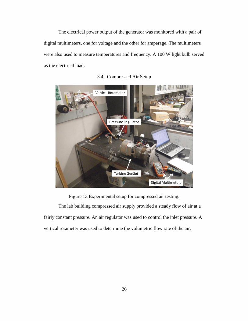
Figure 13 Experimental setup for compressed air testing.
The lab building compressed air supply provided a steady flow of air at a
fairly constant pressure. An air regulator was used to control the inlet pressure. A
vertical rotameter was used to determine the volumetric flow rate of the air.

27
3.5 Steam Setup
Figure 14 Experimental setup for saturated steam testing.
A steam generator was designed and built for testing this Tesla turbine.
This generator is essentially a boiler producing saturated steam. The steam flow
rate was calculated by measuring the change in water amounts contained in the
system over timed intervals. Pressure and temperature gauges provided
measurement readings prior to entering the nozzle. The turbine was oriented with
the exhaust facing down to allow for any condensate to exit the turbine. A
portable air compressor was used to startup the turbine to an RPM approximately
equal to that achieved by the steam at steady-state. This was done to ensure a
more accurate steady-state mass flow rate measurement.
28
3.6 Pressurized Water Setup
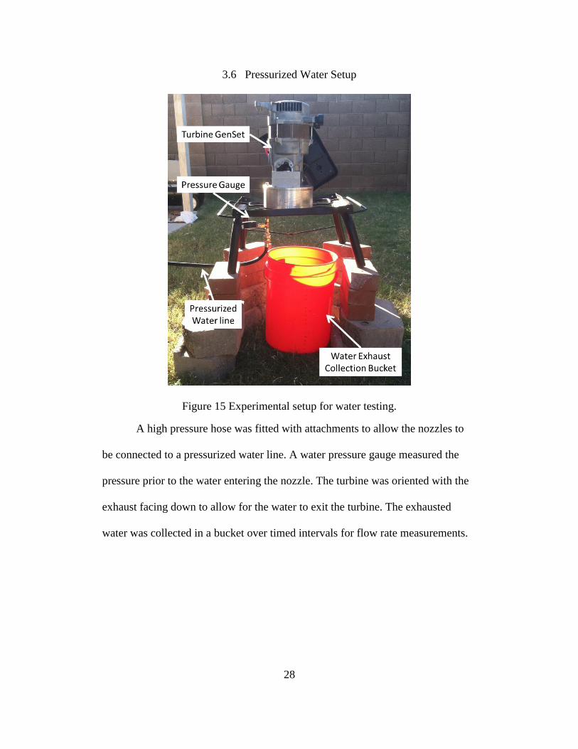
Figure 15 Experimental setup for water testing.
A high pressure hose was fitted with attachments to allow the nozzles to
be connected to a pressurized water line. A water pressure gauge measured the
pressure prior to the water entering the nozzle. The turbine was oriented with the
exhaust facing down to allow for the water to exit the turbine. The exhausted
water was collected in a bucket over timed intervals for flow rate measurements.

29
CHAPTER 4
RESULTS AND DISCUSSION
4.1 Rotor Efficiency
Figure 16 and Figure 17 shows the rotor efficiency plotted against the air
mass flow rate. These plots exhibit an interesting behavior. Initially the efficiency
is low and slowly rises linearly. There is a sudden jump in efficiency that occurs
between 4 and 7 g s-1
. After the sudden jump the efficiency continues to rise,
reaching a maximum value of 95 ± 9.32% for both nozzles (the 101% efficiency
for nozzle 2 obviously being unrealistic). After briefly maintaining peak
efficiency, Figure 16 shows a gradual decline in efficiency. Figure 17 seems to
maintain the peak efficiency.
Although these plots show similar patterns, Figure 16 shows the most
complete plot with the plot in which is then shifted to the right as the nozzle outlet
area increase. The outlet area for nozzle 2 is approximately twice the size of
nozzle 1, apparently causing a small shift of the plot.
Figure 16 Rotor efficiency for nozzle 1 plotted against the mass flow rate for air.

30
Figure 17 Rotor efficiency for nozzle 2 plotted against the mass flow rate for air.
It should be pointed out that the measurement devices used during testing
did not have the sufficient range to capture both plots completely. It would be
interesting to use instruments with the adequate range to determine if the
efficiency stabilizes or continues to drop. From the available data, it appears that
the peak efficiency is maintained over a longer range of mass flow rates with the
larger nozzles; Figure 16 shows the peak efficiency maintained over an
approximately 1gram per second range and Figure 17 maintains the peak
efficiency over a range of at least 2 grams per second.
The peak efficiencies verify Rice’s findings [4] and indicate that a Tesla
turbine with a properly designed nozzle could effectively convert nearly all of the
available energy from the fluid flow once it reaches the rotor. The difficulty will
lie in designing the nozzle to produce the working fluid conditions that will allow
the turbine to meet the load demand while maintaining the high rotor efficiency.
Something to note regarding the impact on the nozzle losses on the efficiencies is
that this impact was minimal. The largest decrease in efficiency was 0.5%,
31
occurring at the peak efficiency and verifying the isentropic assumption. It
appears that this negligible impact would not hold true for much higher fluid
velocities. For the fluid velocities experienced in this testing, the nozzle losses are
negligible and the flow can be modeled as isentropic flow.
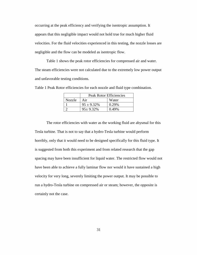
Table 1 shows the peak rotor efficiencies for compressed air and water.
The steam efficiencies were not calculated due to the extremely low power output
and unfavorable testing conditions.
Table 1 Peak Rotor efficiencies for each nozzle and fluid type combination.
Peak Rotor Efficiencies
Nozzle Air Water
1 95 ± 9.32% 0.29%
2 95± 9.32% 0.49%
The rotor efficiencies with water as the working fluid are abysmal for this
Tesla turbine. That is not to say that a hydro-Tesla turbine would perform
horribly, only that it would need to be designed specifically for this fluid type. It
is suggested from both this experiment and from related research that the gap
spacing may have been insufficient for liquid water. The restricted flow would not
have been able to achieve a fully laminar flow nor would it have sustained a high
velocity for very long, severely limiting the power output. It may be possible to
run a hydro-Tesla turbine on compressed air or steam; however, the opposite is
certainly not the case.

32
4.2 Turbine Efficiency
During analysis questions arose concerning the reliability of the rotor
efficiency calculations. Primarily, two main issues were of concern: 1) The flow
conditions at state point 2 could not be verified experimentally; 2) The assumed
value for the other losses of 15% could not be verified. For those reasons, it was
of interest to the author what the highest overall turbine efficiency was for these
experiments and how that efficiency compared to literature results.
Figure 18 and Figure 19 show the overall turbine efficiency plotted against
the air mass flow rate. The behaviors of the curves are very similar to the behavior
seen in Figure 16 and Figure 17 for the rotor efficiencies; however the peak
turbine efficiency only achieved 31.17 ± 3.61% for nozzle 1 and 30.53 ± 3.45%
for nozzle 2 (ignoring, for consistency, the same point that was ignored for the
rotor efficiency for nozzle 2). These peak efficiencies agree quite well with
reported efficiencies in literature [5, 6].
Figure 18 Overall turbine efficiency for nozzle 1 plotted against the mass flow
rate for air.

33
Figure 19 Overall turbine efficiency for nozzle 2 plotted against the mass flow
rate for air.
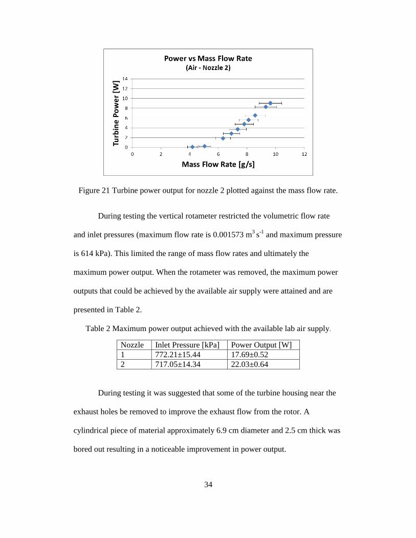
4.3 Power Performance
It can be observed from that as the mass flow rate increased so did the
power output, as one would expect. Figure 20 and Figure 21 show the turbine
work plotted against the mass flow rate. These plots clearly show a sudden
increase in output, occurring between 4-6 g s-1
after which the output increases
linearly.
Figure 20 Turbine power output for nozzle 1 plotted against the mass flow rate.
34
Figure 21 Turbine power output for nozzle 2 plotted against the mass flow rate.
During testing the vertical rotameter restricted the volumetric flow rate
and inlet pressures (maximum flow rate is 0.001573 m3
s-1
and maximum pressure
is 614 kPa). This limited the range of mass flow rates and ultimately the
maximum power output. When the rotameter was removed, the maximum power
outputs that could be achieved by the available air supply were attained and are
presented in Table 2.
Table 2 Maximum power output achieved with the available lab air supply.
Nozzle Inlet Pressure [kPa] Power Output [W]
1 772.21±15.44 17.69±0.52
2 717.05±14.34 22.03±0.64
During testing it was suggested that some of the turbine housing near the
exhaust holes be removed to improve the exhaust flow from the rotor. A
cylindrical piece of material approximately 6.9 cm diameter and 2.5 cm thick was
bored out resulting in a noticeable improvement in power output.

35
4.4 Reynolds Number and Flow Characteristics
Figure 22 and Figure 23 show the turbine efficiency plotted against the
Reynolds number. The behavior is very similar to the other efficiency (rotor or
turbine) curves plotted against the mass flow rate (Figure 16, Figure 17, Figure
18, Figure 19); there is a slight increase in efficiency, followed by a sudden jump,
a peak is reach and then a gradual tapering.
Figure 22 Turbine efficiency for nozzle 1 plotted against the Reynolds number for
air flow.
Figure 23 Turbine efficiency for nozzle 2 plotted against the Reynolds number for
air flow.
36
The results suggest that there are regions of varying fluid flow conditions
that provide some insight into how these conditions impact the overall
performance and efficiency of the Tesla turbine. Figure 22 provides the clearest
view of this changing behavior. The plot can be broken down into four distinct
regions by Reynolds number: 1) up to ~350,000 the behavior is a smooth, low
sloping straight line; 2) between ~350,000 to ~450,000 a sharp jump in efficiency
is achieved; 3) between ~450,000 and ~575,000 the efficiency peaks and is
maintained; and 4) beyond ~575,000 the efficiency begins to taper off slightly.
These regions appear to represent: 1) laminar flow conditions; 2) transitional flow
conditions; 3) mostly turbulent flow conditions; 4) fully turbulent flow conditions.
The Reynolds numbers presented in the plots above are the peak Reynolds
numbers achieved for each test condition. It should be stated that the values for
the higher Reynolds numbers given may not be exact. This is due to the fact that
the estimation for the tangential flow velocity of the fluid is based on laminar
flow assumptions, a flow condition that is not likely to occur at such high
Reynolds numbers. This laminar flow assumption for the tangential velocity
would most likely cause the turbulent Reynolds numbers to be underestimated
because turbulent velocities are likely to be higher than the laminar velocities.
The Reynolds numbers also have a relationship with the outlet area of the
nozzles. When first calculated, the Reynolds numbers for the turbine with nozzle
1 were 1.86 times larger than the numbers for nozzle 2 with nearly identical
efficiencies. The outlet area for nozzle 2 is 1.82 times larger than the area for

37
nozzle 1. As of this report, it is not understood completely why this relationship
exists or what parameters link these values, but it incorporated into the Reynolds
numbers for Figure 23.
Comparisons between Figure 22 and Figure 23 with Figure 20 and Figure
21 indicate that even as the efficiency stops increasing, and in fact, begins to
decrease, the power output continues to climb linearly. This leads to the
conclusion that the presence of turbulent flow, even at the first onset of
transitioning from laminar to turbulent, produces the best power output for the
Tesla turbine.
4.5 Steam Testing Complications
The steam testing encountered a devastating error that could not be
overcome by the date of this paper. The steam generator built for this testing was
accidentally designed to produce a mass flow rate one tenth of the required
amount to achieve maximum power output. This was the result of either bad
communication or incorrect noting of the requirements. Either way, the error was
not discovered until after numerous attempts to increase the rate with the available
materials and equipment failed.
Even though the steam testing did not produce the desired results, it isn’t
difficult to draw the conclusion that saturated steam at similar pressures and flow
rates as compressed air will produce higher outputs. Consider steam and air with
identical flow rates, pressures and temperatures. The two fluid properties that are
most likely to impact the performance of the Tesla turbine are the enthalpy and
the viscosity. The change in enthalpy across the rotor is higher for steam,

38
improving the output, assuming adiabatic conditions. Steam also has a higher
viscosity, improving the transfer of energy from the fluid to the disk for the steam
and, consequently, improving the rotor efficiency.
Table 3 Qualitative comparison of air and steam properties most likely to affect
rotor output and efficiency.
Fluid conditions: Pressure at inlet = 193 kPa
Pressure at outlet = 96.5 kPa
Temperatures are saturation temperatures for the
steam at the given pressures.
Viscosity found at the average temperatures and
pressures.
Fluid Type Change in Enthalpy [kJ kg-1
] Viscosity [N s m-2
106]
Air 20.71 22.18
Steam 86.7 257.6
These qualitative comparisons indicate that the rotor efficiencies for the
steam case should be at least equal to the efficiencies achieved by compressed air.
This conclusion was used to predict necessary inlet pressures and mass flow rates
required to achieve near maximum power outputs for this setup. These projected
results are presented in the following section.
4.6 Projected Saturated Steam Requirements
Table 4 and Table 5 present inlet pressures and mass flow rates that a
steam generator would have to produce in order to achieve the approximate
maximum power output for this experimental setup. The steam generator used in
testing has an experimental mass flow rate ranging from 1.08 to 2.267 g s-1
with
pressures ranging from 141.37 to 196.53 kPa.
These tables and the calculations that created them provide valuable
information for future steam generator advancements. The projected working
fluid conditions are specific to this turbine and the respective nozzles; however,

39
this information coupled with the efficiency and output behavior of the turbine
presented in sections 4.1, 4.2 and 4.3 should be sufficient to design a steam
generator that closely meets the required working fluid conditions at the nozzle
inlet.
Table 4 Projected steam requirements for the turbine using nozzle 1. For these
projections, the turbine is considered adiabatic. These conditions would allow the
generator to produce approximately its maximum power output.
Nozzle 1
Inlet Pressure [kPa] Mass Flow Rate [g/s] Rotor Power Output [W]
273.7 13.3 1205
446.1 16.7 1203
618.4 18.9 1197
790.8 20.4 1198
Table 5 Projected steam requirements for the turbine using nozzle 2. For these
projections, the turbine is considered adiabatic. These conditions would allow the
generator to produce approximately its maximum power output.
Nozzle 2
Inlet Pressure [kPa] Mass Flow Rate [g/s] Rotor Power Output [W]
273.7 16.3 1196
446.1 20.1 1204
618.4 22.3 1204
790.8 23.5 1201

40
CHAPTER 5
FUTURE WORK AND CONCLUSIONS
5.1 Future Turbine Work
The high rotor efficiencies are encouraging indicators of the Tesla
turbine’s potential. The key to advancement toward unlocking that potential
certainly lies in mitigating all other inefficiencies surrounding the rotor. Attention
for future work will only be paid to air and steam working fluids only because the
author has a greater interest in developing gas or steam micro-Tesla turbines for
small scale power production.
The overall turbine efficiencies were comparable to efficiencies reported
in literature, peaking at 31.17 ± 3.61% for nozzle 1 and 30.53 ± 3.45% for nozzle
2. If these efficiencies could be pushed higher as losses are mitigated, especially if
achieved using low quality steam or abrasive-particulate laden heated air, the
applications for the Tesla turbine would be apparent.
Rice pointed out that Tesla turbine nozzles are “necessarily long and
inefficient” [4]. Testing revealed that even slight changes in the nozzle geometry
directly impacted the power produced by the turbine even though the rotor
efficiency stayed relatively high (see Table 1, Figure 16 and Figure 17). Future
work will include designing nozzles specific to the fluid types and desired
pressures, flow rates, velocities, etc. Both converging and converging-diverging
nozzles will be designed to determine whether sonic or super-sonic flow produces
the best output. The relationship between the nozzle geometry and the Reynolds
number should also be investigated to achieve proper design of nozzles.
41
The nozzle losses produce negligible impact on the efficiencies calculated.
This was most likely due to the relatively low fluid velocity and allows for
isentropic flow assumptions to be valid. At much higher fluid velocities the
nozzles losses will have a definite impact on the efficiency and must be accounted
for.
During the testing carried out in this work, turbine insulation was minimal
or non-existent. These conditions did not affect the air and water tests because
heat loss was found to be negligible. However, in the case of steam, heat loss
calculations indicated a substantial loss of overall power for the turbine. Future
work should include properly insulating the turbine before additional steam
testing is carried out.
Exhaust flow losses are another source of inefficiencies that could be
addressed. During testing some improvement was made to the exhaust flow by
removing a cylindrical piece of material from the inner housing wall directly
facing the rotor outlet. This small change created a noted improvement in the
overall power output. Additional improvements to the exhaust flow should be
pursued.
Two ideas for exhaust improvement were formulated and will be
investigated. The first includes staggering the exhaust hole alignment in the disks.
The idea behind this is two-part: one, the staggered holes will allow the turbine to
better capitalize on the rotation motion of the fluid as it approaches the exhaust;
two, in the amount of time it takes for the fluid to reach the adjacent disk, the disk
will have time to rotate to better align the fluid flow with the exhaust hole of the

42
adjacent disk. The second improvement includes fixing the disks to a hollow
shaft. The hollow shaft would have exhaust ports at the disk gaps making the
shaft itself the rotor exhaust.
5.2 Future Steam Generator Work
A new steam generator will need to be designed and built. The results of
this work presented in Table 4 and Table 5 provide much better estimates for the
turbine requirements. Additionally, the specifications will need to be adjusted
especially for any nozzle improvements.
The new steam generator should also include a true superheat stage to
allow for a wider range of steam properties testing. To model a solar thermal
application, the steam generators boiler stage should match the output of
concentrating solar collectors. If the superheat conditions vastly improve the
turbine performance, design of a solar thermal power generator with a
combustible fuel power super heater will be pursued.
5.3 Primary Application: Future Solar Power Unit Work
A solar thermal power unit could be capable of running on low quality,
saturated steam utilizing the Tesla turbine. One of the major benefits of designing
a Rankine system that runs at saturated steam conditions is the significant
reduction in condensing requirements after the turbine. In the testing the steam,
the exhaust fluid temperature was approximately 100 °C and could possibly be air
cooled if an exhaust attachment with high heat transfer capabilities were designed.
Perhaps an aluminum tube fitted with several fins having air forced over it with a
fan.

43
A closed loop design needs to be fully designed to allow for minimal fluid
losses from the system. Once an exhaust attachment is designed, exhaust and inlet
pressures as well as flow rates will be known for selection of an adequate pump.
An air-cooled, closed loop Rankine power system would be an attractive
product especially in arid environments where water scarcity is a serious issue.
5.4 Other Potential Applications to Investigate
A couple of valid questions were asked during review of this paper: “Why
the emphasis on solar thermal power? Given the inexpensive cost of natural gas
these days, would it be better to focus on natural gas powered systems, or perhaps
a hybrid solar thermal/natural gas system?” The answer is definitely. The process
of redesigning the steam generator, which now runs on propane and could just as
easily run on natural gas, will inherently make progress on a combustible gas
fueled system. In fact, the ideal system would include not only a hybrid solar
thermal/natural gas system, but combined heat and power capabilities as well.
This type of setup could eliminate the need for batteries as the primary back up
power source, instead relying on the natural gas to run the system during loss of
solar resources.
5.5 Future Analysis
The discovery of the impact of the flow conditions on the turbine
performance and efficiency is fascinating. Further testing must be performed to
verify the validity of this behavior. North indicated that there may exist a
“turbulent band” around the edge of the turbine disks that is responsible for the
bulk of the power output for the turbine [14]. The velocity profile results from
44
Lampart et al. lend some credence to the possibility of these “turbulent bands”
[8]. The current mathematical model the author used to find the peak Reynolds
numbers used in Figure 22 and Figure 23 is capable of calculating the Reynolds
numbers at various radii of the disks. The results suggest that there is flow
behavior at some radii that could indicate the presence of a “turbulent band”. A
more detailed analysis needs to be performed before these results are made public.
For the needs of this paper, the estimate peak Reynolds numbers suffice.
5.6 Conclusions
The Tesla turbine proved to be versatile prime mover, able to produce
power from a range of working fluids. Experimental test results indicated that this
particular turbine is best suited for ideal gas or steam, but performed poorly as a
hydro-turbine. The ability of this turbine to accept saturated vapor steam gives
merit to the possibility of small-scale Rankine power systems becoming a viable
option for residential scale power production.
The performance of the Tesla turbine was not optimized, but the turbine
rotor efficiency and power outputs were presented for two different nozzles used
in testing. The experiments confirmed that turbine efficiencies can exceed 30%.
An estimated rotor efficiency of 90-95% was also achieved, given certain
assumptions. This moderate turbine efficiency and the potentially outstanding
rotor efficiency is encouraging and further research and development on the
turbine should be pursued to mitigate other sources of inefficiencies limiting the
turbines overall performance.

45
It was determined that turbulence in the flow is essential to achieving high
power outputs and high efficiency. Although the efficiency, after peaking, begins
to slightly taper off as the flow becomes increasingly turbulent, the power output
maintains a steady linear increase.

46
REFERENCES
1. Tesla, N., 1913, “Turbine,” U.S. Patent No. 1,061,206.
2. Hoya, G.P., Guha, A., 2009, “The design of a test rig and study of the
performance and efficiency of a Tesla disc turbine”. Proceedings of the
Institution of Mechanical Engineers, Part A: Journal of Power and Energy,
223, pp. 451-465.
3. The Washington Post, 1912, “Powerful Engine a Mere Toy”, retrieved
from ProQuest Historical Newspapers.
4. Rice, W., 1991, “Tesla Turbomachinery”, Proc. IV International Nikola
Tesla Symposium
5. Guha, A., Smiley, B., 2009, “Experiment and analysis for an improved
design of the inlet and nozzle in Tesla disc turbines”, Proceedings of the
Institution of Mechanical Engineers, Part A: Journal of Power and Energy,
224, pp. 261-277.
6. Lemma, E., Deam, R.T., Toncich, D., Collins, R., 2008, “Characterisation
of a small viscous flow turbine”, Experimental Thermal and Fluid Science,
33, pp. 96-105
7. Tesla, N., 1913, “Fluid Propulsion,” U.S. Patent No. 1,061,142.
8. Lampart, P., Kosowski, K., Piwowarski, M., Jedrzejewski, L., 2009,
“Design analysis of Tesla micro-turbine operating on a low-boiling
medium”, Polish Maritime Research, 16(1), pp. 28-33
9. Fuller, H. J., 2006, “Wind turbine for generation of electric power,” US
Patent No. 7,695,242.
10. Carey, V.P., 2010, “Assessment of Tesla Turbine Performance for Small
Scale Solar Rankine Combined Heat and Power Systems”, Journal of
Engineering for Gas Turbines and Power, 132(12), pp.122301-1 –
122301-8
11. Guha, A., Sengupta, S., 2012, “The fluid dynamics of the rotating flow in
a Tesla disc turbine”. European Journal of Mechanics B/Fluids, 37, pp.
112-123.

47
12. Sengupta, S., Guha, A., 2012, “A theory of Tesla disc turbines”.
Proceedings of the Institution of Mechanical Engineers, Part A: Journal of
Power and Energy, 226(5), pp.650-663.
13. Rice, W., Matsch, L., 1968, “An Asymptotic Solution for Laminar Flow of
an Incompressible Fluid Between Rotating Disks”. Journal of Applied
Mechanics, Series E 90, pp. 155-159.
14. North, R.C., 1969, “An Investigation of the Tesla Turbine”. ProQuest
LLC. University of Maryland.
15. Cirincione, N., 2011, “Design, Construction and Commissioning of an
Organic Rankine Cycle Waste Heat Recovery System with a Tesla-Hybrid
Turbine Expander”. ProQuest LLC. Colorado State University.
16. Rice, W., 1963, “An Analytical and Experimental Investigation of
Multiple Disk Pumps and Compressors”. ASME Trans. J. Eng. Power, 85,
pp. 191-198.
17. Peshlakai, A., Hannoush, E., Marx, J. 2011, “Tesla Turbine Performance”.
Arizona State University.
18. Peshlakai, A., Papachristoforou, D., Anderson, A., Song, E.T., Thomas,
T., 2010, “MAE 488/489 Project: Renewable, Sustainable Energy
Generator”. Arizona State University.
19. Jcmiras.net, 2006, Typical Electric Generator Efficiency, from
http://www.jcmiras.net/jcm/item/93/
20. Cengel, Y.A., Boles, M.A., Thermodynamics An Engineering Approach.
New York: McGraw-Hill, 2008.
21. Moran, M.J., Shapiro, H.N., Munson, B.R., DeWitt, D.P., Introduction to
Thermal Systems Engineering: Thermodynamics, Fluid Mechanics, and
Heat Transfer. New Jersey: John Wiley & Sons, Inc, 2003.
22. Panton, R.L., Incompressible Flow. New Jersey: John Wiley & Sons, Inc,
2009.
23. Lee, T.W., Thermal and Flow Measurements. New York: CRC Press,
2008.

48
APPENDIX A
TABLE OF UNCERTAINTIES FOR MEASUREMENT DEVICES

49
Table 6 Uncertainties for measurement devices used during testing. The
uncertainty values were reported by the device manufacturer.
Measurement Device Variable Uncertainty,
Digital Multimeter Voltage ±1.5% of reading
Digital Multimeter Current ±2.5% of reading
Digital Multimeter with Thermocouple Temperature ± 3% of reading
Graduated Beaker Fluid Volume ± 10 mL
Calipers Length ± 0.025 mm
Vertical Rotometer Volumetric Flow
rate
± 3% of reading
Steam Pressure/Temperature Gauge Temperature
Pressure
± 2% of reading
Air Pressure Gauge Pressure ± 2% of reading