Ch 6. Oligopoly

September 19, 2015

Ch 6. Oligopoly

§6.1. Oligopoly: Bertrand competition

TCi (qi ) = c · qi , c > 0 – marginal cost.Linear demand function:

Q = D(p) = a− bp, p ∈ [0,a

b].

Demand function for the 1st firm:

q1 = D1(p1, p2) =

a− bp1, p1 < p2;12(a− bp1), p1 = p2;0, p1 > p2.

(6.1.1)

Ch 6. Oligopoly

Payoff functions of competing firms:{πi (pi , p3−i ) = (pi − c) · Di (pi , p3−i ) −→ max

pi;

pi ≥ 0.(6.1.2)

Th 6.1.1.

There exists unique NE p∗1 = p∗2 = c in Bertrand duopoly(oligopoly) symmetric model, and both firm’s profits are equal zero(Bertrand paradox).

Ch 6. Oligopoly

Payoff functions of competing firms:{πi (pi , p3−i ) = (pi − c) · Di (pi , p3−i ) −→ max

pi;

pi ≥ 0.(6.1.2)

Th 6.1.1.

There exists unique NE p∗1 = p∗2 = c in Bertrand duopoly(oligopoly) symmetric model, and both firm’s profits are equal zero(Bertrand paradox).

Ch 6. Oligopoly

§6.2. Cournot duopoly (linear demand functions)

Both firms simultaneously choose their outputs q1 ≥ 0 and q2 ≥ 0.Total output: q = q1 + q2.Inverse demand function:

p(q) = p(q1 + q2) = max{a− bq, 0}, (6.2.1)

where a and b – positive parameters.Marginal costs:

MC1 = MC2 = c, 0 ≤ c < a, (6.2.2)

assume zero fixed costs.

Ch 6. Oligopoly

§6.2. Cournot duopoly (linear demand functions)

Both firms simultaneously choose their outputs q1 ≥ 0 and q2 ≥ 0.Total output: q = q1 + q2.Inverse demand function:

p(q) = p(q1 + q2) = max{a− bq, 0}, (6.2.1)

where a and b – positive parameters.Marginal costs:

MC1 = MC2 = c , 0 ≤ c < a, (6.2.2)

assume zero fixed costs.

Ch 6. Oligopoly

The 1-st firm profit maximization problem:{π1(q1, q2) = q1 · p(q1 + q2)− cq1 −→ max

q1;

q1 ≥ 0.(6.2.3)

Profit is positive iff:

a− b(q1 + q2) < c .

Then:{π1(q1, q2) = q1 · (a− c − b(q1 + q2)) −→ max

q1;

0 ≤ q1 ≤ a−cb − q2.

(6.2.4)

Ch 6. Oligopoly

The 1-st firm profit maximization problem:{π1(q1, q2) = q1 · p(q1 + q2)− cq1 −→ max

q1;

q1 ≥ 0.(6.2.3)

Profit is positive iff:

a− b(q1 + q2) < c .

Then:{π1(q1, q2) = q1 · (a− c − b(q1 + q2)) −→ max

q1;

0 ≤ q1 ≤ a−cb − q2.

(6.2.4)

Ch 6. Oligopoly

The problem (6.2.4) solution for given firm’s 2 outputq2 ∈ [0, a−c

b ) denote by q1 = R1(q2).

q1 = R1(q2), q2 ∈ [0,a− c

b)

Reaction function (or Best response function) of the 1-st firm.

Given q2 the 1-st firm reaction function R1(q2) shows such 1-stfirm output value q1, which maximises her profit.

Ch 6. Oligopoly

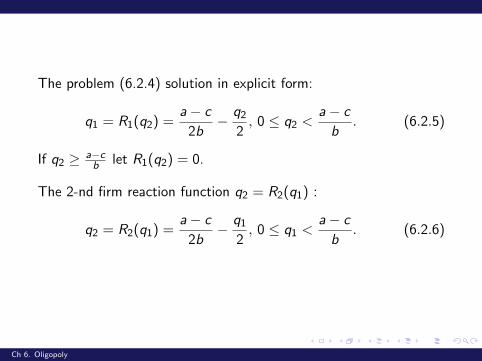
The problem (6.2.4) solution in explicit form:

q1 = R1(q2) =a− c

2b− q2

2, 0 ≤ q2 <

a− c

b. (6.2.5)

If q2 ≥ a−cb let R1(q2) = 0.

The 2-nd firm reaction function q2 = R2(q1) :

q2 = R2(q1) =a− c

2b− q1

2, 0 ≤ q1 <

a− c

b. (6.2.6)

Ch 6. Oligopoly

The problem (6.2.4) solution in explicit form:

q1 = R1(q2) =a− c

2b− q2

2, 0 ≤ q2 <

a− c

b. (6.2.5)

If q2 ≥ a−cb let R1(q2) = 0.

The 2-nd firm reaction function q2 = R2(q1) :

q2 = R2(q1) =a− c

2b− q1

2, 0 ≤ q1 <

a− c

b. (6.2.6)

Ch 6. Oligopoly

The graphs of reaction functions - Reaction curves.

6

-0 q1

q2

a−cb

a−c2b

a−c2b

a−c4b

a−cb

HHHHH

HHHHHH

H

AAAAAAAAAAAA

R1(q2)

Cq

S1q

R2(q1)

HHHHH

HHHHHH

H

HHHHH

HHHHHH

H

HHHHH

HHHHHH

H

HHHHH

HHHHHH

H

AAAAAAAAAAAA

AAAAAAAAAAAA

AAAAAAAAAAAA

AAAAAAAAAAAA

Fig. 6.2.1. Reaction curves, Cournot and Stakelberg equilibriums (in strategy space Oq1q2)

Ch 6. Oligopoly

The solution (q∗1 , q∗2) of the system (6.2.5) and (6.2.6) is called

Cournot equilibrium.

q∗1 = q∗2 =a− c

3b. (6.2.7)

Note that:

p∗ = p(q∗1 + q∗2) =1

3(a + 2c) (6.2.8)

– market price,

πc1 = πc2 = πi (q∗1 , q

∗2) =

(a− c)2

9b(6.2.9)

– the firm profit.

Ch 6. Oligopoly

The solution (q∗1 , q∗2) of the system (6.2.5) and (6.2.6) is called

Cournot equilibrium.

q∗1 = q∗2 =a− c

3b. (6.2.7)

Note that:

p∗ = p(q∗1 + q∗2) =1

3(a + 2c) (6.2.8)

– market price,

πc1 = πc2 = πi (q∗1 , q

∗2) =

(a− c)2

9b(6.2.9)

– the firm profit.

Ch 6. Oligopoly

6

-0 π1

π2

t/9 t/8 t/4

t/9

t/16

t/4@@@@@@@@@@@@

rrrCπ

S1π

Fig. 6.2.2. Cournot and Stackelberg equilibriums

(in payoff functions space Oπ1π2), (a−c)2

b = t

Property 6.2.1. Cournot equilibrium (q∗1 , q∗2) is NE.

Ch 6. Oligopoly

6

-0 π1

π2

t/9 t/8 t/4

t/9

t/16

t/4@@@@@@@@@@@@

rrrCπ

S1π

Fig. 6.2.2. Cournot and Stackelberg equilibriums

(in payoff functions space Oπ1π2), (a−c)2

b = t

Property 6.2.1. Cournot equilibrium (q∗1 , q∗2) is NE.

Ch 6. Oligopoly

§6.3. Stackelberg equilibrium, collusion, ...

Stackelberg model (quantity leadership).Consider a two-stage game in which one firm (leader) gets to movefirst. The other firm (follower) then observes the leader’s outputand chooses its own output using best response function.

Let firm 1 be the leader and firm 2 be the follower.

The leader’s profit maximization problem:{π1(q1,R2(q1)) −→ max

q1;

q1 ≥ 0.(6.3.1)

The solution q̄1 of (6.3.1) – the leader’s optimal output,q̄2 = R2(q̄1) – the follower’s optimal output, (q̄1, q̄2) – Stackelbergequilibrium.

Ch 6. Oligopoly

§6.3. Stackelberg equilibrium, collusion, ...

Stackelberg model (quantity leadership).Consider a two-stage game in which one firm (leader) gets to movefirst. The other firm (follower) then observes the leader’s outputand chooses its own output using best response function.

Let firm 1 be the leader and firm 2 be the follower.

The leader’s profit maximization problem:{π1(q1,R2(q1)) −→ max

q1;

q1 ≥ 0.(6.3.1)

The solution q̄1 of (6.3.1) – the leader’s optimal output,q̄2 = R2(q̄1) – the follower’s optimal output, (q̄1, q̄2) – Stackelbergequilibrium.

Ch 6. Oligopoly

§6.3. Stackelberg equilibrium, collusion, ...

Stackelberg model (quantity leadership).Consider a two-stage game in which one firm (leader) gets to movefirst. The other firm (follower) then observes the leader’s outputand chooses its own output using best response function.

Let firm 1 be the leader and firm 2 be the follower.

The leader’s profit maximization problem:{π1(q1,R2(q1)) −→ max

q1;

q1 ≥ 0.(6.3.1)

The solution q̄1 of (6.3.1) – the leader’s optimal output,q̄2 = R2(q̄1) – the follower’s optimal output, (q̄1, q̄2) – Stackelbergequilibrium.

Ch 6. Oligopoly

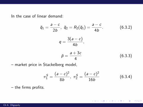
In the case of linear demand:

q̄1 =a− c

2b, q̄2 = R2(q̄1) =

a− c

4b. (6.3.2)

q =3(a− c)

4b,

p̄ =a + 3c

4(6.3.3)

– market price in Stackelberg model,

πS1 =(a− c)2

8b, πS2 =

(a− c)2

16b(6.3.4)

– the firms profits.

Ch 6. Oligopoly

Other possible patterns of firm behavior (duopoly settings):

collusion;

both firms choose their output like a follower in Stackelbergmodel;

both firms choose their output like a leader in Stackelbergmodel.

Ch 6. Oligopoly

The collusion scheme:

qm = q1 + q2 =a− c

2b, q1 ≥ 0, q2 ≥ 0,

optimal monopoly price pm = a+c2 , maximal total profit

πm = π1 + π2 =(a− c)2

4b.

There are many strategy profiles (q1, q2), that satisfy(q1 + q2 = qm), but no profile satisfies NE.

Ch 6. Oligopoly

The collusion scheme:

qm = q1 + q2 =a− c

2b, q1 ≥ 0, q2 ≥ 0,

optimal monopoly price pm = a+c2 , maximal total profit

πm = π1 + π2 =(a− c)2

4b.

There are many strategy profiles (q1, q2), that satisfy(q1 + q2 = qm), but no profile satisfies NE.

Ch 6. Oligopoly

The followers scheme:

q1 = q2 =a− c

4b.

Total output q = a−c2b , market prise coincides with monopoly price

pm = a+c2 , each firm profit:

π1 = π2 =(a− c)2

8b.

This strategy profile dominates (Pareto dominates) the Cournot

equilibrium (πci = (a−c)2

9b ), however does not satisfy NE.

Ch 6. Oligopoly

The followers scheme:

q1 = q2 =a− c

4b.

Total output q = a−c2b , market prise coincides with monopoly price

pm = a+c2 , each firm profit:

π1 = π2 =(a− c)2

8b.

This strategy profile dominates (Pareto dominates) the Cournot

equilibrium (πci = (a−c)2

9b ), however does not satisfy NE.

Ch 6. Oligopoly

The leaders scheme:

q1 = q2 =a− c

2b.

Total output: q = a−cb , market price: p = c, both firms get zero

profit.

Ch 6. Oligopoly