wireless network pricing chapter 6: oligopoly...
TRANSCRIPT
Wireless Network PricingChapter 6: Oligopoly Pricing
Jianwei Huang & Lin Gao
Network Communications and Economics Lab (NCEL)Information Engineering DepartmentThe Chinese University of Hong Kong
Huang & Gao ( c�NCEL) Wireless Network Pricing: Chapter 6 November 15, 2016 1 / 69
The Book
E-Book freely downloadable from NCEL website: http://ncel.ie.cuhk.edu.hk/content/wireless-network-pricing
Physical book available for purchase from Morgan & Claypool(http://goo.gl/JFGlai) and Amazon (http://goo.gl/JQKaEq)
Huang & Gao ( c�NCEL) Wireless Network Pricing: Chapter 6 November 15, 2016 2 / 69
Section 6.3:Wireless Service Provider Competition Revisited
Huang & Gao ( c�NCEL) Wireless Network Pricing: Chapter 6 November 15, 2016 45 / 69
Network Model
Provider 1
Provider 2
Provider 3
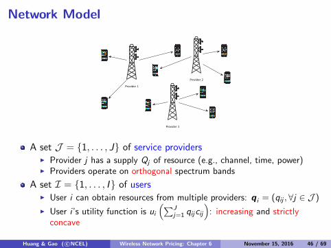
A set J = {1, . . . , J} of service providersI Provider j has a supply Qj of resource (e.g., channel, time, power)I Providers operate on orthogonal spectrum bands
A set I = {1, . . . , I} of usersI User i can obtain resources from multiple providers: q i = (qij , 8j 2 J )
I User i ’s utility function is ui⇣PJ
j=1
qijcij⌘: increasing and strictly
concave
Huang & Gao ( c�NCEL) Wireless Network Pricing: Chapter 6 November 15, 2016 46 / 69
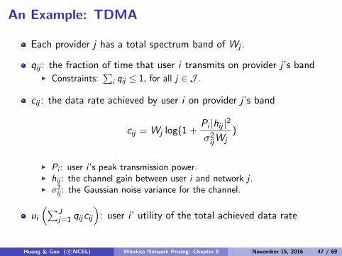
An Example: TDMA
Each provider j has a total spectrum band of Wj .
qij : the fraction of time that user i transmits on provider j ’s bandI Constraints:
Pi qij 1, for all j 2 J .
cij : the data rate achieved by user i on provider j ’s band
cij = Wj log(1 +Pi |hij |2�2
ijWj)
I Pi : user i ’s peak transmission power.I hij : the channel gain between user i and network j .I �2
ij : the Gaussian noise variance for the channel.
ui⇣PJ
j=1
qijcij⌘: user i ’ utility of the total achieved data rate
Huang & Gao ( c�NCEL) Wireless Network Pricing: Chapter 6 November 15, 2016 47 / 69
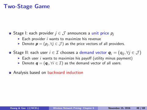
Two-Stage Game
Stage I: each provider j 2 J announces a unit price pjI Each provider i wants to maximize his revenueI Denote p = (pj , 8j 2 J ) as the price vectors of all providers.
Stage II: each user i 2 I chooses a demand vector q i = (qij , 8j 2 J )I Each user i wants to maximize his payo↵ (utility minus payment)I Denote q = (q i , 8i 2 I) as the demand vector of all users.
Analysis based on backward induction
Huang & Gao ( c�NCEL) Wireless Network Pricing: Chapter 6 November 15, 2016 48 / 69
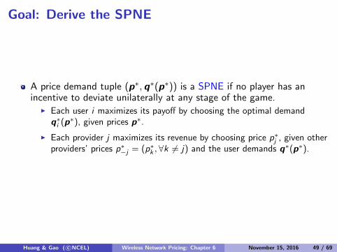
Goal: Derive the SPNE
A price demand tuple (p⇤,q⇤(p⇤)) is a SPNE if no player has anincentive to deviate unilaterally at any stage of the game.
I Each user i maximizes its payo↵ by choosing the optimal demandq⇤i (p⇤), given prices p⇤.
I Each provider j maximizes its revenue by choosing price p⇤j , given otherproviders’ prices p⇤�j = (p⇤k , 8k 6= j) and the user demands q⇤(p⇤).
Huang & Gao ( c�NCEL) Wireless Network Pricing: Chapter 6 November 15, 2016 49 / 69
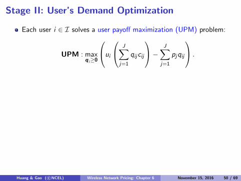
Stage II: User’s Demand Optimization
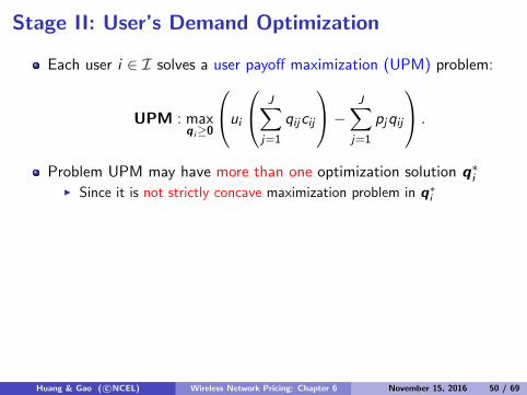
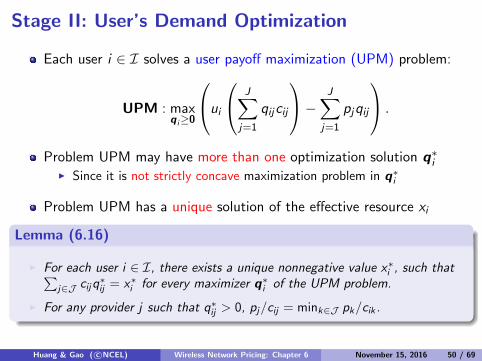
Each user i 2 I solves a user payo↵ maximization (UPM) problem:
UPM : maxq i�0
0
@ui
0
@JX
j=1
qijcij
1
A�JX
j=1
pjqij
1
A .
Problem UPM may have more than one optimization solution q⇤i
I Since it is not strictly concave maximization problem in q⇤i
Problem UPM has a unique solution of the e↵ective resource xi
Lemma (6.16)
I For each user i 2 I, there exists a unique nonnegative value x⇤i , such thatPj2J cijq⇤ij = x⇤i for every maximizer q⇤
i of the UPM problem.
I For any provider j such that q⇤ij > 0, pj/cij = mink2J pk/cik .
Huang & Gao ( c�NCEL) Wireless Network Pricing: Chapter 6 November 15, 2016 50 / 69
Stage II: User’s Demand Optimization
Each user i 2 I solves a user payo↵ maximization (UPM) problem:
UPM : maxq i�0
0
@ui
0
@JX
j=1
qijcij
1
A�JX
j=1
pjqij
1
A .
Problem UPM may have more than one optimization solution q⇤i
I Since it is not strictly concave maximization problem in q⇤i
Problem UPM has a unique solution of the e↵ective resource xi
Lemma (6.16)
I For each user i 2 I, there exists a unique nonnegative value x⇤i , such thatPj2J cijq⇤ij = x⇤i for every maximizer q⇤
i of the UPM problem.
I For any provider j such that q⇤ij > 0, pj/cij = mink2J pk/cik .
Huang & Gao ( c�NCEL) Wireless Network Pricing: Chapter 6 November 15, 2016 50 / 69
Decided vs. Undecided Users
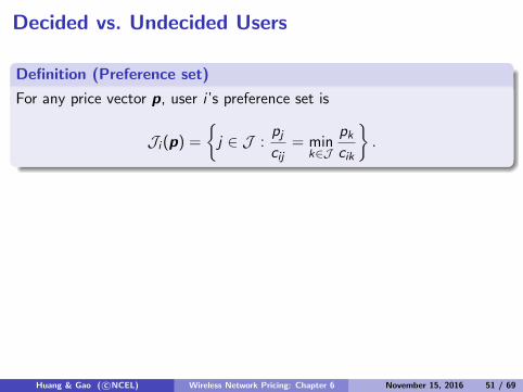
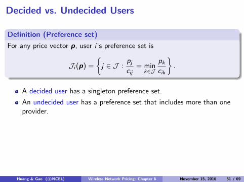
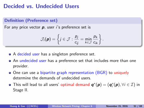
Definition (Preference set)
For any price vector p, user i ’s preference set is
Ji (p) =⇢j 2 J :
pjcij
= mink2J
pkcik
�.
A decided user has a singleton preference set.
An undecided user has a preference set that includes more than oneprovider.
One can use a bipartite graph representation (BGR) to uniquelydetermine the demands of undecided users.
This will lead to all users’ optimal demand q⇤(p) = (q⇤i (p), 8i 2 I) in
Stage II.
Huang & Gao ( c�NCEL) Wireless Network Pricing: Chapter 6 November 15, 2016 51 / 69
Decided vs. Undecided Users
Definition (Preference set)
For any price vector p, user i ’s preference set is
Ji (p) =⇢j 2 J :
pjcij
= mink2J
pkcik
�.
A decided user has a singleton preference set.
An undecided user has a preference set that includes more than oneprovider.
One can use a bipartite graph representation (BGR) to uniquelydetermine the demands of undecided users.
This will lead to all users’ optimal demand q⇤(p) = (q⇤i (p), 8i 2 I) in
Stage II.
Huang & Gao ( c�NCEL) Wireless Network Pricing: Chapter 6 November 15, 2016 51 / 69

Stage I: Provider’s Revenue Optimization
Each provider j 2 J solves a provider revenue maximization (PRM)problem
PRM : maxpj�0
pj ·min
Qj ,X
i2Iq⇤ij(pj , p�j)
!
Solving the PRM problem requires the consideration of otherproviders’ prices p�j .
Huang & Gao ( c�NCEL) Wireless Network Pricing: Chapter 6 November 15, 2016 52 / 69
Benchmark: Social Welfare Optimization (Ch. 4)
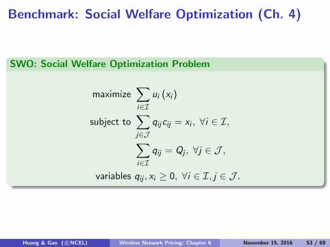
SWO: Social Welfare Optimization Problem
maximizeX
i2Iui (xi )
subject toX
j2Jqijcij = xi , 8i 2 I,
X
i2Iqij = Qj , 8j 2 J ,
variables qij , xi � 0, 8i 2 I, j 2 J .
Huang & Gao ( c�NCEL) Wireless Network Pricing: Chapter 6 November 15, 2016 53 / 69
Stage I: Provider’s Revenue Optimization
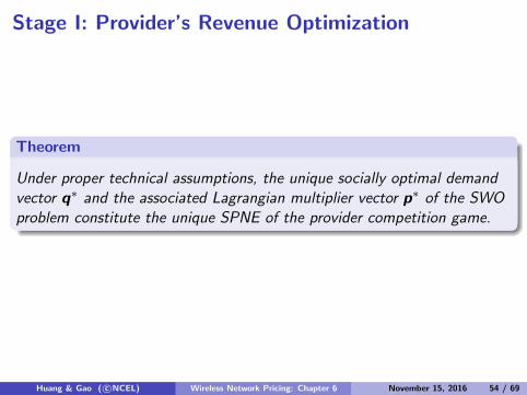
Theorem
Under proper technical assumptions, the unique socially optimal demandvector q⇤ and the associated Lagrangian multiplier vector p⇤ of the SWOproblem constitute the unique SPNE of the provider competition game.
Huang & Gao ( c�NCEL) Wireless Network Pricing: Chapter 6 November 15, 2016 54 / 69
Optimization, Game, and Algorithm
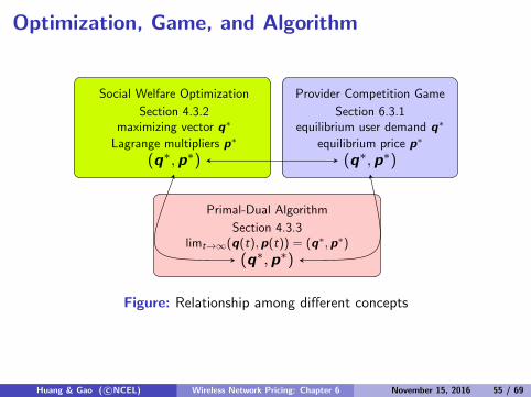
Social Welfare Optimization
Section 4.3.2maximizing vector q⇤
Lagrange multipliers p⇤
(q⇤,p⇤)
Provider Competition Game
Section 6.3.1
equilibrium price p⇤equilibrium user demand q⇤
(q⇤,p⇤)
Primal-Dual Algorithm
Section 4.3.3limt!1(q(t),p(t)) = (q⇤,p⇤)
(q⇤,p⇤)
Figure: Relationship among di↵erent concepts
Huang & Gao ( c�NCEL) Wireless Network Pricing: Chapter 6 November 15, 2016 55 / 69
Section 6.4:Competition with Spectrum Leasing
Huang & Gao ( c�NCEL) Wireless Network Pricing: Chapter 6 November 15, 2016 56 / 69
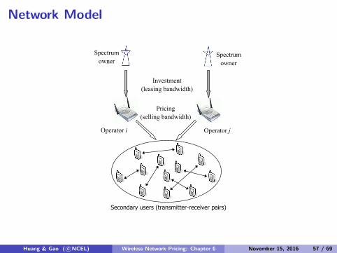
Network Model
Secondary users (transmitter-receiver pairs)
Spectrum owner
Operator i Operator j
Investment (leasing bandwidth)
Pricing (selling bandwidth)
Spectrum owner
Huang & Gao ( c�NCEL) Wireless Network Pricing: Chapter 6 November 15, 2016 57 / 69
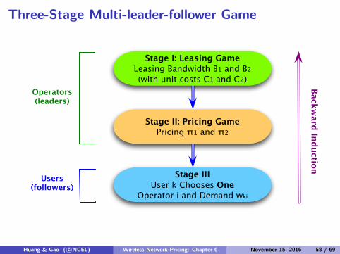
Three-Stage Multi-leader-follower Game
Stage I: Leasing Game
Leasing Bandwidth B1 and B2
(with unit costs C1 and C2)
Stage II: Pricing Game
Pricing π1 and π2
Stage III
User k Chooses One
Operator i and Demand wki
Operators(leaders)
Users(followers)
Backw
ard
Ind
uctio
n
Huang & Gao ( c�NCEL) Wireless Network Pricing: Chapter 6 November 15, 2016 58 / 69
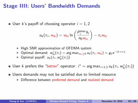
Stage IIII: Users’ Bandwidth Demands
User k ’s payo↵ of choosing operator i = 1, 2
uk(⇡i ,wki ) = wki ln
✓Pmax
i hin0
wki
◆� ⇡iwki
I High SNR approximation of OFDMA systemI Optimal demand: w⇤
ki (⇡i ) = argmaxwki�0
uk(⇡i ,wki ) = gke�(1+⇡i )
I Optimal payo↵: uk(⇡i ,w⇤ki (⇡i ))
User k prefers the “better” operator: i⇤ = argmaxi=1,2 uk(⇡i ,w⇤ki (⇡i ))
Users demands may not be satisfied due to limited resourceI Di↵erence between preferred demand and realized demand
Huang & Gao ( c�NCEL) Wireless Network Pricing: Chapter 6 November 15, 2016 59 / 69
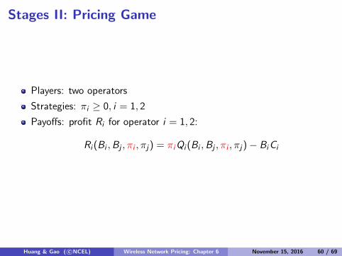
Stages II: Pricing Game
Players: two operators
Strategies: ⇡i � 0, i = 1, 2
Payo↵s: profit Ri for operator i = 1, 2:
Ri (Bi ,Bj ,⇡i ,⇡j) = ⇡iQi (Bi ,Bj ,⇡i ,⇡j)� BiCi
Huang & Gao ( c�NCEL) Wireless Network Pricing: Chapter 6 November 15, 2016 60 / 69
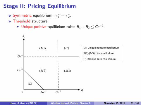
Stage II: Pricing Equilibrium
Symmetric equilibrium: ⇡⇤1
= ⇡⇤2
.
Threshold structure:I Unique positive equilibrium exists B
1
+ B2
Ge�2.
( 1)M
( 3)M
( )L
( 2)M
( )H
0
2Ge−
1Ge−
iB
jB
2Ge− 1Ge−
(L) : Unique nonzero equilibrium
(M1)‐(M3) : No equilibrium
(H) : Unique zero equilibrium
Huang & Gao ( c�NCEL) Wireless Network Pricing: Chapter 6 November 15, 2016 61 / 69
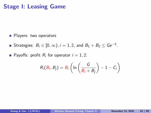
Stage I: Leasing Game
Players: two operators
Strategies: Bi 2 [0,1), i = 1, 2, and B1
+ B2
Ge�2.
Payo↵s: profit Ri for operator i = 1, 2:
Ri (Bi ,Bj) = Bi
✓ln
✓G
Bi + Bj
◆� 1� Ci
◆
Huang & Gao ( c�NCEL) Wireless Network Pricing: Chapter 6 November 15, 2016 62 / 69
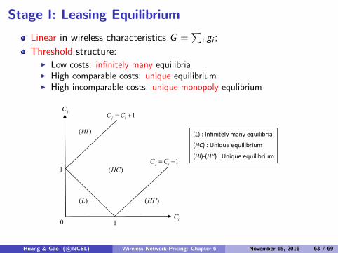
Stage I: Leasing Equilibrium
Linear in wireless characteristics G =P
i gi ;
Threshold structure:I Low costs: infinitely many equilibriaI High comparable costs: unique equilibriumI High incomparable costs: unique monopoly equlibrium
1j iC C= +
( )L
1
10 iC
jC
( )HC
( )HI
( ')HI
1j iC C= −
(L) : Infinitely many equilibria
(HC) : Unique equilibrium
(HI)‐(HI’) : Unique equilibrium
Huang & Gao ( c�NCEL) Wireless Network Pricing: Chapter 6 November 15, 2016 63 / 69
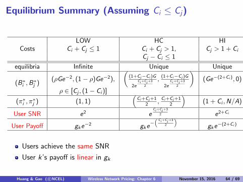
Equilibrium Summary (Assuming Ci Cj)
CostsLOW HC HI
Ci + Cj 1 Ci + Cj > 1, Cj > 1 + Ci
Cj � Ci 1
equilibria Infinite Unique Unique
(B⇤i ,B
⇤j )
(⇢Ge�2, (1� ⇢)Ge�2),
✓(1+Cj�Ci )G
2eCi+Cj+3
2
, (1+Ci�Cj )G
2eCi+Cj+3
2
◆(Ge�(2+Ci ), 0)
⇢ 2 [Cj , (1� Ci )]
(⇡⇤i ,⇡
⇤j ) (1, 1)
⇣Ci+Cj+1
2
, Ci+Cj+1
2
⌘(1 + Ci ,N/A)
User SNR e2 eCi+Cj+3
2 e2+Ci
User Payo↵ gke�2 gke�⇣
Ci+Cj+3
2
⌘
gke�(2+Ci )
Users achieve the same SNR
User k ’s payo↵ is linear in gk
Huang & Gao ( c�NCEL) Wireless Network Pricing: Chapter 6 November 15, 2016 64 / 69
Robustness of Results
To obtain closed form solutions, we have assumedI All users achieve high SNR
Previous observations still hold in the general case
I Users operate in general SNR regime: rki (wki ) = wki ln⇣1 + Pmax
k hkn0
wki
⌘
Huang & Gao ( c�NCEL) Wireless Network Pricing: Chapter 6 November 15, 2016 65 / 69

Impact of Duopoly Competition on OperatorsBenchmark: Coordinated Case
I Operators cooperate in investment and pricing to maximize total profit
Define
E�ciency Ratio =Total Profit in Competition Case
Total Profit in Coordinated CasePrice of Anarchy = minCi ,Cj E�ciency Ratio= 0.75.
Huang & Gao ( c�NCEL) Wireless Network Pricing: Chapter 6 November 15, 2016 66 / 69
Section 6.5: Chapter Summary
Huang & Gao ( c�NCEL) Wireless Network Pricing: Chapter 6 November 15, 2016 67 / 69
Key Concepts
Theory: Game TheoryI Dominant StrategyI Pure and Mixed Strategy Nash EquilibriumI Subgame Perfect Nash Equilibrium
Theory: OligopolyI Cournot competitionI Bertrand competitionI Hotelling competition
Application: Wireless Network Competition Revisited
Application: Competition with Spectrum Leasing
Huang & Gao ( c�NCEL) Wireless Network Pricing: Chapter 6 November 15, 2016 68 / 69
References and Extended Reading
J. Huang, “How Do We Play Games?” online video tutorial, on YouKu(http://www.youku.com/playlist_show/id_19119535.html) andiTunesU (https://itunes.apple.com/hk/course/how-do-we-play-games/id642100914)
V. Gajic, J. Huang, and B. Rimoldi, “Competition of Wireless Providers for
Atomic Users,” IEEE Transactions on Networking, vol. 22, no. 2, pp. 512 -
525, April 2014
L. Duan, J. Huang, and B. Shou, “Duopoly Competition in DynamicSpectrum Leasing and Pricing,” IEEE Transactions on MobileComputing, vol. 11, no. 11, pp. 1706 1719, November 2012
http://ncel.ie.cuhk.edu.hk/content/wireless-network-pricing
Huang & Gao ( c�NCEL) Wireless Network Pricing: Chapter 6 November 15, 2016 69 / 69