c:/documents and settings/lrouxj/my …
TRANSCRIPT
DSC2606/1
Study Guide
Nonlinear Mathematical Programming
DSC2606
Department of Decision Sciences
IMPORTANT INFORMATION
Please register on myUnisa, activate your myLife e-mail address and
make sure that you have regular access to the myUnisa module
website, as well as your group website.
Bar code
c©2017 Department of Decision Sciences,University of South Africa.
All rights reserved.
Printed and distributed by theUniversity of South Africa,Muckleneuk, Pretoria.
DSC2606/1
Contents
Chapter 1 Basics 3
1.1 Historical background . . . . . . . . . . . . . . . . . . . . . . 4
1.2 The scientific approach . . . . . . . . . . . . . . . . . . . . . 5
1.3 What is a model? . . . . . . . . . . . . . . . . . . . . . . . . 6
1.4 What does a mathematical model look like? . . . . . . . . . . 7
1.5 Mathematical programming and linear programming . . . . .9
1.6 Properties and assumptions of linear programming . . . . .. 9
1.7 Other operations research techniques . . . . . . . . . . . . . . 10
Chapter 2 Introducing linear programming models 13
2.1 Types of problem . . . . . . . . . . . . . . . . . . . . . . . . 14
2.2 Mark’s LP model . . . . . . . . . . . . . . . . . . . . . . . . 16
2.3 Christine’s LP model . . . . . . . . . . . . . . . . . . . . . . 18
2.4 Components of an LP model . . . . . . . . . . . . . . . . . . 20
2.5 General LP model . . . . . . . . . . . . . . . . . . . . . . . . 22
Chapter 3 Graphical representation 23
3.1 A graphical approach . . . . . . . . . . . . . . . . . . . . . . 24
3.2 Finding the feasible area . . . . . . . . . . . . . . . . . . . . 25
3.3 Identifying the optimal solution . . . . . . . . . . . . . . . . . 29
3.4 Solving Christine’s problem graphically . . . . . . . . . . . .35
3.5 Types of solution . . . . . . . . . . . . . . . . . . . . . . . . 38
3.5.1 Infeasible LPs . . . . . . . . . . . . . . . . . . . . . . 38
3.5.2 Unbounded solutions . . . . . . . . . . . . . . . . . . 38
iii

DSC2606
CONTENTS
3.5.3 Multiple optimal solutions . . . . . . . . . . . . . . . 40
3.5.4 Degenerate solutions . . . . . . . . . . . . . . . . . . 41
3.6 Types of constraint . . . . . . . . . . . . . . . . . . . . . . . 42
3.6.1 Redundant constraints . . . . . . . . . . . . . . . . . 42
3.6.2 Binding and nonbinding constraints . . . . . . . . . . 42
3.7 Exercises . . . . . . . . . . . . . . . . . . . . . . . . . . . . 43
3.8 Solutions to exercises . . . . . . . . . . . . . . . . . . . . . . 44
Chapter 4 Computer solutions 49
4.1 Introduction . . . . . . . . . . . . . . . . . . . . . . . . . . . 50
4.2 Using LINGO . . . . . . . . . . . . . . . . . . . . . . . . . . 50
4.3 Solving Mark’s problem with LINGO . . . . . . . . . . . . . 51
4.4 Solving Christine’s problem with LINGO . . . . . . . . . . . 53
4.5 Exercises . . . . . . . . . . . . . . . . . . . . . . . . . . . . 54
4.6 Solutions to exercises . . . . . . . . . . . . . . . . . . . . . . 54
Chapter 5 Introductory concepts 59
5.1 Introduction . . . . . . . . . . . . . . . . . . . . . . . . . . . 60
5.2 Linear versus nonlinear . . . . . . . . . . . . . . . . . . . . . 61
5.3 Examples of NLP categories . . . . . . . . . . . . . . . . . . 62
5.4 Assumptions of NLP . . . . . . . . . . . . . . . . . . . . . . 63
5.5 Solutions to models – basic concepts . . . . . . . . . . . . . . 64
5.6 Exercises . . . . . . . . . . . . . . . . . . . . . . . . . . . . 64
5.7 Solutions to exercises . . . . . . . . . . . . . . . . . . . . . . 65
Chapter 6 Formulating NLP models and computer solutions 67
6.1 Introduction . . . . . . . . . . . . . . . . . . . . . . . . . . . 68
6.2 A dimensions problem . . . . . . . . . . . . . . . . . . . . . 68
6.3 An inventory problem . . . . . . . . . . . . . . . . . . . . . . 70
6.4 LINGO . . . . . . . . . . . . . . . . . . . . . . . . . . . . . 71
6.5 Formulation and LINGO solution of NLP models . . . . . . . 74
6.6 Exercises . . . . . . . . . . . . . . . . . . . . . . . . . . . . 75
iv
CONTENTS
DSC2606
6.7 Solutions to exercises . . . . . . . . . . . . . . . . . . . . . . 75
6.8 Looking ahead at the remaining study units . . . . . . . . . . 77
Chapter 7 Limits and continuity 79
7.1 Introduction . . . . . . . . . . . . . . . . . . . . . . . . . . . 80
7.2 The limit of a function . . . . . . . . . . . . . . . . . . . . . 80
7.3 Infinite limits . . . . . . . . . . . . . . . . . . . . . . . . . . 90
7.4 Limits whenx tends to infinity . . . . . . . . . . . . . . . . . 92
7.5 Continuity . . . . . . . . . . . . . . . . . . . . . . . . . . . . 94
7.6 Exercises . . . . . . . . . . . . . . . . . . . . . . . . . . . . 97
7.7 Solutions to exercises . . . . . . . . . . . . . . . . . . . . . . 101
Chapter 8 The derivative of a function 103
8.1 Introduction . . . . . . . . . . . . . . . . . . . . . . . . . . . 104
8.2 The slope of a tangent line . . . . . . . . . . . . . . . . . . . 106
8.3 The rate of change . . . . . . . . . . . . . . . . . . . . . . . 109
8.4 The derivative of a function . . . . . . . . . . . . . . . . . . . 109
8.5 Differentiability and continuity . . . . . . . . . . . . . . . . . 114
8.6 Exercises . . . . . . . . . . . . . . . . . . . . . . . . . . . . 115
8.7 Solutions to exercises . . . . . . . . . . . . . . . . . . . . . . 117
Chapter 9 The rules of differentiation 119
9.1 Four basic rules . . . . . . . . . . . . . . . . . . . . . . . . . 120
9.2 The product rule . . . . . . . . . . . . . . . . . . . . . . . . . 125
9.3 The derivative of the exponential function . . . . . . . . . . .125
9.4 The derivative of the logarithmic function . . . . . . . . . . .126
9.5 Higher-order derivatives . . . . . . . . . . . . . . . . . . . . 127
9.6 The chain rule . . . . . . . . . . . . . . . . . . . . . . . . . . 128
9.7 Exercises . . . . . . . . . . . . . . . . . . . . . . . . . . . . 133
9.8 Solutions to exercises . . . . . . . . . . . . . . . . . . . . . . 134
v
DSC2606
CONTENTS
Chapter 10 Properties of functions and sketching graphs 137
10.1 Introduction . . . . . . . . . . . . . . . . . . . . . . . . . . . 138
10.2 Increasing and decreasing functions . . . . . . . . . . . . . . 138
10.3 Relative and absolute extrema . . . . . . . . . . . . . . . . . 141
10.4 Concavity . . . . . . . . . . . . . . . . . . . . . . . . . . . . 148
10.5 The second derivative test . . . . . . . . . . . . . . . . . . . . 152
10.6 Asymptotes . . . . . . . . . . . . . . . . . . . . . . . . . . . 154
10.7 Sketching graphs . . . . . . . . . . . . . . . . . . . . . . . . 157
10.8 Exercises . . . . . . . . . . . . . . . . . . . . . . . . . . . . 160
10.9 Solutions to exercises . . . . . . . . . . . . . . . . . . . . . . 161
Chapter 11 Zeros of functions or roots of equations 167
11.1 Introduction . . . . . . . . . . . . . . . . . . . . . . . . . . . 168
11.2 Locating roots of equations . . . . . . . . . . . . . . . . . . . 168
11.3 Bisection method . . . . . . . . . . . . . . . . . . . . . . . . 170
11.3.1 Computer algorithms . . . . . . . . . . . . . . . . . . 173
11.4 Newton’s method . . . . . . . . . . . . . . . . . . . . . . . . 176
11.4.1 Computer algorithms . . . . . . . . . . . . . . . . . . 179
11.5 Exercises . . . . . . . . . . . . . . . . . . . . . . . . . . . . 182
11.6 Solutions to exercises . . . . . . . . . . . . . . . . . . . . . . 183
Chapter 12 Marginal analysis 185
12.1 Introduction . . . . . . . . . . . . . . . . . . . . . . . . . . . 186
12.2 Cost functions . . . . . . . . . . . . . . . . . . . . . . . . . . 186
12.3 Average cost functions . . . . . . . . . . . . . . . . . . . . . 189
12.4 Revenue functions . . . . . . . . . . . . . . . . . . . . . . . . 192
12.5 Profit functions . . . . . . . . . . . . . . . . . . . . . . . . . 194
12.6 Exercises . . . . . . . . . . . . . . . . . . . . . . . . . . . . 195
12.7 Solution to exercises . . . . . . . . . . . . . . . . . . . . . . 195
vi
CONTENTS
DSC2606
Chapter 13 Optimisation of NLPs in one variable 199
13.1 Introduction . . . . . . . . . . . . . . . . . . . . . . . . . . . 200
13.2 Vital theorems . . . . . . . . . . . . . . . . . . . . . . . . . . 200
13.3 Solving NLPs in one variable by differential calculus .. . . . 201
13.4 Returning to LINGO . . . . . . . . . . . . . . . . . . . . . . 206
13.5 Exercises . . . . . . . . . . . . . . . . . . . . . . . . . . . . 207
13.6 Solutions to exercises . . . . . . . . . . . . . . . . . . . . . . 208
Chapter 14 Golden section search 213
14.1 Introduction . . . . . . . . . . . . . . . . . . . . . . . . . . . 214
14.2 The golden section search . . . . . . . . . . . . . . . . . . . . 214
14.3 Exercises . . . . . . . . . . . . . . . . . . . . . . . . . . . . 219
14.4 Solutions to exercises . . . . . . . . . . . . . . . . . . . . . . 219
Chapter 15 Integration 223
15.1 Introduction . . . . . . . . . . . . . . . . . . . . . . . . . . . 224
15.2 Antiderivatives . . . . . . . . . . . . . . . . . . . . . . . . . 224
15.3 The indefinite integral . . . . . . . . . . . . . . . . . . . . . . 227
15.4 The basic rules of integration . . . . . . . . . . . . . . . . . . 228
15.5 Integration by substitution . . . . . . . . . . . . . . . . . . . 233
15.6 The area under the graph of a function . . . . . . . . . . . . . 237
15.7 The fundamental theorem of calculus . . . . . . . . . . . . . . 241
15.8 The method of substitution for definite integrals . . . . .. . . 245
15.9 Consumers’ and producers’ surplus . . . . . . . . . . . . . . . 248
15.9.1 Consumers’ surplus . . . . . . . . . . . . . . . . . . . 248
15.9.2 Producers’ surplus . . . . . . . . . . . . . . . . . . . 248
15.10Numerical integration . . . . . . . . . . . . . . . . . . . . . . 251
15.10.1 Trapezoidal rule . . . . . . . . . . . . . . . . . . . . 252
15.10.2 Computer algorithm for trapezoidal rule . . . . . . . . 254
15.11Exercises . . . . . . . . . . . . . . . . . . . . . . . . . . . . 256
15.12Solutions to exercises . . . . . . . . . . . . . . . . . . . . . . 257
vii
DSC2606
CONTENTS
Chapter 16 Partial differentiation 263
16.1 Introduction . . . . . . . . . . . . . . . . . . . . . . . . . . . 264
16.2 Partial derivatives . . . . . . . . . . . . . . . . . . . . . . . . 266
16.3 Second-order partial derivatives . . . . . . . . . . . . . . . . 272
16.4 The Cobb-Douglas production function . . . . . . . . . . . . 275
16.5 Exercises . . . . . . . . . . . . . . . . . . . . . . . . . . . . 277
16.6 Solutions to exercises . . . . . . . . . . . . . . . . . . . . . . 277
Chapter 17 Optimisation of NLPs in several variables 281
17.1 Introduction . . . . . . . . . . . . . . . . . . . . . . . . . . . 282
17.2 Convex and concave functions . . . . . . . . . . . . . . . . . 283
17.3 Stationary points and the nature of stationary points .. . . . . 287
17.4 Solving NLPs in several variables by differential calculus . . . 289
17.5 Exercises . . . . . . . . . . . . . . . . . . . . . . . . . . . . 293
17.6 Solutions to exercises . . . . . . . . . . . . . . . . . . . . . . 294
Chapter 18 Method of steepest ascent 301
18.1 Introduction . . . . . . . . . . . . . . . . . . . . . . . . . . . 302
18.2 The method of steepest ascent . . . . . . . . . . . . . . . . . 302
18.3 The method of steepest descent . . . . . . . . . . . . . . . . . 306
18.4 Exercises . . . . . . . . . . . . . . . . . . . . . . . . . . . . 306
18.5 Solutions to exercises . . . . . . . . . . . . . . . . . . . . . . 306
Chapter 19 Lagrange multipliers 309
19.1 The method of Lagrange multipliers . . . . . . . . . . . . . . 310
19.2 Verification . . . . . . . . . . . . . . . . . . . . . . . . . . . 312
19.3 Exercises . . . . . . . . . . . . . . . . . . . . . . . . . . . . 313
19.4 Solutions to exercises . . . . . . . . . . . . . . . . . . . . . . 313
Chapter 20 Kuhn-Tucker conditions 317
20.1 Kuhn-Tucker conditions . . . . . . . . . . . . . . . . . . . . 318
20.2 Exercises . . . . . . . . . . . . . . . . . . . . . . . . . . . . 322
20.3 Solutions to exercises . . . . . . . . . . . . . . . . . . . . . . 322
viii
Part 1
Linear Programming
This part introduces the concept of mathematical programming. Thenotes are a summary of the part on linear programming in the studyguide of the module DSC2605. This background is necessary forplacing nonlinear programming in context and for understanding theuse of LINGO to solve mathematical programming problems.Youmust familiarise yourself with this background to mathematicalprogramming, but you will not be examined explicitly on the studyunits in this part.
1

2
Chapter 1
Basics
Contents1.1 Historical background . . . . . . . . . . . . . . . . . . . 4
1.2 The scientific approach . . . . . . . . . . . . . . . . . . 5
1.3 What is a model? . . . . . . . . . . . . . . . . . . . . . . 6
1.4 What does a mathematical model look like? . . . . . . . 7
1.5 Mathematical programming and linear programming . 9
1.6 Properties and assumptions of linear programming . . 9
1.7 Other operations research techniques . . . . . . . . . . 10
3

DSC2606
CHAPTER 1 BASICS
Sections from prescribed book,WinstonChapter 1Chapter 3, Section 3.1
Learning objectivesAfter completing this study unit you should be able to
• explain what “operations research” is
• describe how the scientific approach is applied to Operations Re-search/Quantitative Management
• explain what a mathematical model is
• explain what “mathematical programming” is
• explain what “linear programming” is
• give the properties and assumptions of linear programming
• give examples of operations research techniques and their areas ofapplication.
1.1 Historical background
In the period between the two great wars, military technology developed byleaps and bounds without military leaders having the chanceto apply all thenew weapons together or to experiment with new weapon systems. Whenthe German air attacks on England started during World War II, some of theBritish military managers and leaders recognised this factand realised thatthey were confronted with problems for which there were no parallels inhistory.
In order to maximise their war effort, the British government organisedteams of scientific and engineering personnel to assist fieldcommanders insolving perplexing strategic and tactical problems. They found that techni-cally trained men could solve problems outside their normalprofessionalcompetency. They asked biologists to examine problems in electronics,physicists to think in terms of the movement of people ratherthan the move-ment of molecules, mathematicians to apply probability theory to improvesoldiers’ chances of survival, and chemists to study equilibria in systemsother than in chemicals. Teams made up of specialists from these differentdisciplines studied problems ranging from the evaluation of cost and effec-tiveness of complete military systems (such as the defence system of a coun-try) to the best placement of depth charges in anti-submarine warfare.
4
1.2. THE SCIENTIFIC APPROACH
DSC2606
The success of the British operational research teams led the United Statesto institute a similar effort in 1942 (small-scale projectsdated back to 1937).The initial project involved the deployment of merchant marine convoys tominimise losses from enemy submarines.
These mathematical and scientific approaches to military operations werethen calledoperations research.
The success of operations research techniques during the Second World Warled to the techniques being extended and applied to other fields after the war.
Today the term “operations research” means a scientific approach to decisionmaking, which seeks to determine how best to design and operate a system,usually under conditions requiring the allocation of scarce resources.
Operations research is now applied so extensively in many areas that a sep-arate discipline has been established. The diversity of this discipline has ledto its being known not only asoperations research, but also by terms suchasmanagement science, decision science, decision analysisandquantitativemanagement.
1.2 The scientific approach
Descartes, a French philosopher and mathematician of the 17th century, em-phasised the use of reason as the chief tool of enquiry. The scientific ap-proach, also known as the scientific method, is a formalised reasoning pro-cess. It consists of the following steps:
(a) The problem for analysis is defined, and the conditions for observationare determined.
(b) Observations are made under different conditions to determine thebehaviour of the system containing the problem.
(c) Based on the observations, a hypothesis that describes how the fac-tors involved are thought to interact, or what the best solution to theproblem is, is conceived.
(d) An experiment is designed to test the hypothesis.
(e) The experiment is carried out, and measurements are obtained andrecorded.
(f) The results of the experiment are analysed, and the hypothesis is eitheraccepted or rejected.
The six steps of the scientific method can be applied to decision making ingeneral and to Operations Research/Quantitative Management in particular,and can be adapted for this purpose as follows:
• identify the problem
5
DSC2606
CHAPTER 1 BASICS
• collect the relevant data
• construct a mathematical model to represent the problem
• select a solution method
• derive a solution to the model
• test the model and evaluate the solution
• implement and maintain the solution.
There can be interaction between these steps.
1.3 What is a model?
A model is a representation of a real entity, and may be constructed in orderto gain some understanding of, or insight into, that entity.A model should berealistic enough to incorporate the important characteristics of the real-lifesystem it represents, but not so complex as to hide those characteristics.
Three types of model are generally distinguished:
• Iconic models are physical representations of real objects, designed toresemble those objects in appearance. For example, when a tall build-ing is planned, engineers may construct a small-scale modelof thatbuilding, and of its surrounding area and environment, in order to con-duct stress tests in a wind tunnel.
• Analogue models are also physical models, but represent theentitiesunder study by analogue rather than by replica. An example isa graphshowing the movements over time of stock market prices; thistype ofmodel provides a pictorial representation of numerical data.
• Mathematical models, or symbolic models, are more abstractrepre-sentations than iconic or analogue models. They attempt to provide,for example, through an equation or system of equations, a descriptionof a real-life system.
Operations research makes extensive use of mathematical models. To beused successfully, a mathematical model must meet the following criteria:
(a) The model should be as simple and understandable as possible.
(b) The model should be reasonable. Its structures should constrain an-swers to a reasonable range of values and make it difficult forunrealis-tic answers to result from inputs.
(c) The model should be easy to maintain.
(d) The model should be adaptive. The parameters and structures of themodel should be easy to change as new insights and information evolve.
6
1.4. WHAT DOES A MATHEMATICAL MODEL LOOK LIKE?
DSC2606
(e) The model should be complete on important issues.
1.4 What does a mathematical model look like?
Consider a business that manufactures and sells a product. The product costsR5 to manufacture and sells for R20. A model that computes thetotal profitthat will accrue from the items sold is given by the followingequation:
Z = 20x−5x.
Here x represents the number of units of the product that are manufactured andsold, and
Z represents the total profit in rand that will result from the sale of theproduct.
The symbols,x andZ, are referred to as variables. The termvariable isused because no set numerical value has been specified for these items. Thenumber of units manufactured and sold and the resulting profit can be anyamount (within limits) – they can vary.
These two variables can be further distinguished as follows:
• The variableZ is known as adependentvariable because its value isdependent on the number of units manufactured and sold.
• The variablex is anindependentvariable, since the number of unitsmanufactured and sold is not dependent upon anything else (in thismodel). It is also called thedecision variable, because its value is usu-ally determined by a conscious decision made by someone withtheauthority to do so.
The numbers 20 and 5 in the equation are referred to asparameters.Param-eters are constant values that are generally coefficients ofthe variables in anequation. Parameters may change in the longer term but usually remain con-stant for the duration of solving a specific problem, for example, the price ofthe product may change over time but is fixed for the time being.
The equation as a whole is known as afunctional relationship.This termis derived from the fact that profit,Z, is afunctionof the number of unitsmanufactured and sold,x.
Since only one functional relationship exists in this example, it is also themodel. This model does not represent a real problem – it merely states afunctional relationship in a mathematical form – and we expand our exampleto create a problem situation.
Let us assume that the product is made from steel and that 500 grams ofsteel is needed to make one unit of the product, and that a total of 100 kilo-grams of steel is available for production.
7
DSC2606
CHAPTER 1 BASICS
If one unit of the product uses 500 grams of steel, then the total number ofproducts manufactured,x, uses 500×x grams of steel, or 0,5x kilograms ofsteel.
The steel used to manufacture the products may obviously notexceed thesteel available for production. A mathematical inequalityrepresenting thisrelationship between steel used and steel available can nowbe developedand is as follows:
0,5x≤ 100 (steel utilisation in kilograms).
The “less than or equal to” sign,≤, is used asno more than100 kilogramsmay be used.
A negative number of products can obviously not be manufactured and thiscan be expressed mathematically asx≥ 0. The “greater than or equal to”sign,≥, is used asat leastzero units of the product must be manufactured.
The model now consists of three relationships:
Z = 20x−5x
0,5x ≤ 100
x ≥ 0.
To add some flavour to the model, we now assume that a manager, say theproduction manager, must decide on the number of units of theproduct tomanufacture. What objective do you think he will have in mindwhen havingto decide on this? Surely to achieve as much profit as possible. The ideal isan infinite profit, but this cannot be reached in practice because of the lim-ited availability of steel. Based on this observation we cannow make a dis-tinction between the relationships in the model.
The equationZ = 20x−5x represents profit and is called theobjective func-tion of the model. The inequality 0,5x≤ 100 represents the steel utilisationand is called the resourceconstraint. The inequalityx≥ 0 specifies the nu-merical values that the variablex may assume. It is also a constraint and iscalled thesign restriction.
To emphasise the distinction between the objective function and the con-straints, the model is written as follows:
Maximise Z = 20x−5x
subject to
0,5x≤ 100
and x≥ 0.
This is an example of a very simple model.
8
1.5. MATHEMATICAL PROGRAMMING AND LINEAR PROGRAMMING
DSC2606
1.5 Mathematical programming and linear pro-gramming
In the world of quantitative analysis, the word “programming” refers to themodelling and solvingof practical problems. “Modelling” refers to the con-struction of a model to represent a problem situation. Our interest is in ma-thematical models.
“Mathematical programming” therefore means the construction of mathe-matical models of real-life problem situations and their solutions. All mathe-matical programming models consist of an objective function that has to bemaximised or minimised, and a set of constraints.
“Linear programming” is one category of mathematical programming. Lin-ear programming models are distinguished by the fact that the objectivefunction and the constraints are linear. This means that each term in an equa-tion or inequality is either a number or a number multiplied by a symbol.There are no squares, cubes, cross-products or other funny things present.Linear programming is often denoted by LP and in this guide wewill followthis convention.
From the above we see that the word “programming” has a special mean-ing and should not be confused with computer programming. Computerprogramming has, however, played an important role in the advancementand use of operations research techniques. Most real-life problems are toocomplex to solve by hand or even with a calculator, and require the use ofcomputer packages.
1.6 Properties and assumptions of linear pro-gramming
Linear programming has been applied extensively in the pastto military, in-dustrial, financial, marketing, accounting and agricultural problems. TodayLP continues to be used in many different fields and even though the appli-cations are so diverse, all LP problems have four propertiesin common.
Linear programming problems have the followingproperties:
(a) All problems seek to optimise (maximise or minimise) some quantity(usually profit or cost). This property is referred to as theobjectiveofthe problem. This objective must be clearly stated and mathematicallydefined in the form of an objective function.
(b) There are restrictions, calledconstraints, on the problem. These con-straints limit the degree to which the objective of the problem can bepursued.
9
DSC2606
CHAPTER 1 BASICS
(c) There arealternative courses of actionto choose from. Say, for ex-ample, a company manufactures three different products. Then man-agement must decide how to allocate its limited production resourcesbetween the three products.
(d) The objective and constraints of a problem are expressedas equationsand inequalities and each of these islinear.
Linear programming is based on the followingassumptions:
(a) Certainty. This means that all the parameters (numerical values) in theobjective function and constraints are known with certainty and do notchange during the period being studied.
(b) Proportionality. Proportionality exists in the objective function andconstraints. Say, for example, that the production of one unit of aproduct uses three hours of a resource. Then making 10 units of theproduct will use 10×3 hours of the resource.
(c) Additivity. This means that the total of all activities equals the sumof the individual activities. Say, for example, that the objective is tomaximise the profit resulting from the sale of two products. And theprofit contribution of the first product is R5 and the profit contributionof the second product is R7. Then the total profit resulting from themanufacture of one unit of each product will be R5+R7= R12.
(d) Divisibility. This means that the actual values of the decision variablesneed not be in whole numbers (integers). But they may take on frac-tional values, that is, they are divisible. For example, theproductionof 10,4 computers per day is quite acceptable since the productionprocess is continuous. The rest of the eleventh computer canbe com-pleted on the following day. If integer answers are requiredfor practi-cal purposes, rounding off the values to the nearest integers may yieldreasonable results.
Sometimes a fractional solution is not acceptable and an integer solu-tion must be forced. In this case, the model must specify thatan inte-ger solution is required and this is called integer programming. Integerprogramming will not be discussed in this module.
1.7 Other operations research techniques
LP is just part of the vast number of techniques available forproblem solv-ing and decision making that form part of the tool kit provided by operationsresearch. A few others are inventory control techniques, network techniques(network flow, CPM/PERT), probabilistic techniques (game theory, markovanalysis, simulation, forecasting, etc.), nonlinear programming and otherlinear techniques such as integer and goal programming.
10

1.7. OTHER OPERATIONS RESEARCH TECHNIQUES
DSC2606
A schematic representation of some of the techniques of operations researchand their areas of application is given in Figure 1.1.
O P E R A T I O N S R E S E A R C H T E C H N I Q U E S
M a t h e m a t i c a l
p r o g r a m m i n g
D e c i s i o n
a n a l y s i s
N e t w o r k s I n v e n t o r y
c o n t r o l
S t o c h a s t i c
m o d e l l i n g
Linear programming
Nonlinear programming
Int eger programmi ng
Goal programmi ng
Dynamic programming
Multi-criteria decision m
aking
Expert systems
Rout ing
Project scheduling
Queuing theory
Si m
ul at ion
Forecasting
G e n e r a l
m a n a g e m e n t
O p e r a t i o n s
m a n a g e m e n t
F i n a n c i a l
m a n a g e m e n t
M a r k e t i n g
m a n a g e m e n t
Q u a l i t y
m a n a g e m e n t
S t r a t e g i c
m a n a g e m e n t
E n v i r o n m e n t a l
m a n a g e m e n t
Figure 1.1: A schematic representation
11

DSC2606
CHAPTER 1 BASICS
12

Chapter 2
Introducing linear programmingmodels
Contents2.1 Types of problem . . . . . . . . . . . . . . . . . . . . . . 14
2.2 Mark’s LP model . . . . . . . . . . . . . . . . . . . . . 16
2.3 Christine’s LP model . . . . . . . . . . . . . . . . . . . 18
2.4 Components of an LP model . . . . . . . . . . . . . . . 20
2.5 General LP model . . . . . . . . . . . . . . . . . . . . . 22
13
DSC2606
CHAPTER 2 INTRODUCING LINEAR PROGRAMMING MODELS
Sections from prescribed book,WinstonChapter 3, Section 3.1
Learning objectivesAfter completing this study unit you should be able to
• identify all the components of an LP model
• write down the general LP model.
2.1 Types of problem
Mark and Christine, a young, up-and-coming professional couple, are dis-cussing the events of the day. Mark is an engineer whose team has devel-oped a new television projection system. Final tests have just been success-fully completed and the results are encouraging. The systemwill be installedon two models, theVH200 and theSB150. Although very excited, Mark isalso a bit worried. “I wish we had a larger work force, more machine timeand better marketing capabilities. I am sure we could make a fat profit. Butas it is, we don’t even know how many of each model to manufacture.”
Christine has problems of her own at the Unique Paint Company. A newexpensive special purpose paint, Sungold, is becoming verypopular. Theproduction manager has asked Christine to see if she can find acombina-tion of two new ingredients, code-named Alpha and Beta, thatwill result inthe same brilliance and tint as the original ingredients; but at a lower cost.Christine feels confident that she can.
Christine does not realise that her problem, a typicalblendingproblem, is inmany ways equivalent to Mark’s, a typicalproduct-mixproblem.
Resource allocation problems appear in several forms. Examples are givenbelow.
Product-mix problems
Most manufacturing companies are capable of producing morethan oneproduct and have the ability to adjust, to some extent at least, the propor-tions in which products are made. The objective is to choose the product mixthat is most profitable. In making this choice, the firm will beconstrained byits resources of equipment and labour, material, finances, etc.
Blending problems
Many products, for example those of the chemical, petroleum, pharmaceu-tical and processed food industries, contain mixtures of basic ingredients.
14
2.1. TYPES OF PROBLEM
DSC2606
The finished product must meet certain specifications. Subject to these be-ing met, the manufacturer is free to choose the blend of basicingredients,being constrained by their availability. The choice made aims at producing asatisfactory product at minimum cost.
Transportation problems
A company, for example, a textbook publisher, may have warehouses atvarious places in the country. All orders received from bookshops must besupplied by these warehouses. For example, copies of textbooks must beshipped to campus bookstores to meet the demand there. The company willwant to minimise the distribution costs while meeting this demand.
Purchasing problems
The purchasing department of a company has access to different raw mate-rials in various quantities and qualities. They can buy these in a number ofdifferent combinations. And they are subject to productionrequirements andbudget restrictions. They want to find the combination with the lowest cost.
Portfolio selection problems
An investor must decide how to distribute his investments among alternativeassets, such as common stocks and bonds, in order to maximiseexpectedreturn.
Advertising media mix problems
The marketing department of a company must decide how much tospendon advertising in newspapers and magazines and on radio and television.They are restricted by the given budget for production promotion, and theavailable media space and time. The objective is to maximisethe exposureof the product to potential customers.
Production and inventory scheduling problems
Manufacturing companies face variations in the market demand for theirproducts. As it is generally costly to make changes to production schedules,inventory is carried to help meet fluctuations in demand. Theproblem is tominimise production and inventory holding costs, while meeting anticipatedproduct demand.
The range of applications is diverse, but we can trace the following twocommon threads:
• Each of the applications involves optimisation, whether itis to max-imise or to minimise something.
• Optimisation is always subject to constraints on what is possible.
Many practical management problems can be characterised asproblems ofconstrained optimisation.
15
DSC2606
CHAPTER 2 INTRODUCING LINEAR PROGRAMMING MODELS
2.2 Mark’s LP model
The television manufacturing company is in the market to make money –its objective is to maximise profit. A profit of R300 is made on each set ofmodelVH200 sold and R250 on each set of modelSB150 sold.
We can see that the moreVH200 sets manufactured and sold, the better.However, there are certain limitations which prevent the company from man-ufacturing and selling thousands ofVH200 models.
These limitations are as follows:
• there are only 40 hours of labour time available per day for production
• there are only 45 hours of machine time available per day
• there is an inability to sell more than 12 sets of modelVH200 per day.
To manufacture one set of modelVH200, two hours of labour time and onehour of machine time is required. To manufacture one set of modelSB150,one hour of labour time and three hours of machine time is required.
Mark’s problem is to determine how many sets of each model to manufac-ture each day so that the total profit will be as large as possible.
Let us formulate his problem as an LP model.
Decision variables
What decisions must be made?
Mark must decide how many modelVH200 and how many modelSB150television sets to manufacture each day. These decisions can be representedby the followingdecision variables:
VH = number of modelVH200 sets to manufacture daily,
SB = number of modelSB150 sets to manufacture daily.
The decision variables used when formulating models shouldcompletelydescribe the decisions to be made.
Objective function
The objective is to maximise profit.
This objective can be expressed in the form of a function of the decisionvariables and is then called an objective function.
Proportionality is assumed, and this means that since the profit contributionof one set of modelVH200 is R300, then the profit contribution ofVH unitsof this model is300×VH.
16
2.2. MARK’S LP MODEL
DSC2606
Similarly, the profit resulting from the manufacture ofSBunits of modelSB150 is 250×SB.
The total profit is therefore 300VH+250SB. The objective function is then
MaximisePROFIT= 300VH+250SB.
Constraints
What limitations, or restrictions, are there on the problem?
The labour and machine time is limited and there are restricted marketingcapabilities. This means that there are limited resources.These resourcesrestrict the number of television sets that can be manufactured. These re-strictions are calledconstraints.
Labour constraint
One modelVH200 set requires two hours of labour time and the unknownquantityVH requires 2×VH hours. Similarly 1×SBhours of labour time isrequired to manufacture the modelSB150 sets.
The total labour time required is therefore 2VH+SB.
There are 40 labour hours available for manufacturing the television sets.
The labour time used may not be more than the available labourhours. Thiscan be expressed as
labour hours required≤ labour hours available
labour hoursVH200+ labour hoursSB150 ≤ labour hours available
2VH+SB ≤ 40.
Note the≤ sign. The total number of labour hours available, 40, need notnecessarily all be used.
Machine constraint
The machine constraint can be deduced in a similar way as
VH+3SB≤ 45.
Marketing constraint
The marketing capabilities are restricted and the result ofthis is that it isimpossible to sell more than 12 sets of modelVH200 daily. This constraintis represented as
VH ≤ 12.
17
DSC2606
CHAPTER 2 INTRODUCING LINEAR PROGRAMMING MODELS
Sign restrictions
It is impossible to manufacture a negative number of television sets and soVH andSBmust be nonnegative. These constraints are expressed as
VH ≥ 0; SB≥ 0.
The LP model for Mark’s problem is
Maximise PROFIT= 300VH+250SB
subject to
2VH + SB ≤ 40 (Labour time)
VH + 3SB ≤ 45 (Machine time)
VH ≤ 12 (Marketing)
and VH; SB≥ 0.
NOTE:Since production continues day after day, it is not necessary to com-plete all sets at the end of the day. A fractional number of sets is permissible(e.g. 5,7 sets). However, had it been necessary to complete all sets by theend of the day, additional constraints limitingVH andSBto whole numberswould have been added. Such an addition changes the problem to one of in-teger programming, which will not be discussed in this module.
2.3 Christine’s LP model
In preparing Sungold paint it is required that the paint has abrilliance ratingof at least 300 degrees and a tint level of at least 250 degrees. Brilliance andtint levels are determined by the two ingredients, Alpha andBeta.
Each gram of Alpha produces one degree of brilliance in a tin of paint. Like-wise for Beta. However, the tint is controlled entirely by the amount of Al-pha, one gram of it producing three degrees of tint in one tin of paint.
The cost of Alpha is 45 cents per gram and the cost of Beta is 12 cents pergram.
Assuming that the objective is to minimise the cost of the ingredients, theproblem is to find the quantity of Alpha and Beta to be includedin the prepa-ration of each tin of paint. An optimal answer for one tin willremain opti-mal for any number of tins as long as the relationships are linear. The totalquantity of paint to be produced is of course more than one tin, and it is de-termined mainly by the demand and the manufacturing technology formula-tion.
18
2.3. CHRISTINE’S LP MODEL
DSC2606
Decision variables
The decision variables are
ALPHA = quantity (in grams) of Alpha in each tin of paint,
BETA = quantity (in grams) of Beta in each tin of paint.
Objective function
The objective is to minimise the total cost of the ingredients.
Since the cost of Alpha is 45 cents per gram and sinceALPHAgrams are tobe used in each tin, the cost per tin is 45×ALPHA. Similarly for Beta, thecost is 12×BETA.
The total cost is 45ALPHA+12BETA, and the objective function is given by
MinimiseCOST= 45ALPHA+12BETA.
Constraints
Brilliance constraint
Each gram of Alpha produces one degree of brilliance in a tin of paint andsoALPHAgrams of Alpha produces 1×ALPHAdegrees of brilliance. Sim-ilarly BETAgrams of Beta produces 1×BETAdegrees of brilliance in a tinof paint.
The total brilliance produced in a tin of paint by the two ingredients is then
ALPHA+BETA.
A brilliance rating of at least 300 degrees per tin is required.
The brilliance produced must be at least the brilliance required. This can beexpressed as
brilliance produced≥ brilliance required
brilliance from Alpha+ brilliance from Beta ≥ brilliance required
ALPHA+BETA ≥ 300.
Tint constraint
The tint constraint can be deduced in a similar way as
tint produced ≥ tint required
tint from Alpha+ tint from Beta ≥ tint required
3×ALPHA+0×BETA ≥ 250
3ALPHA ≥ 250.
19
DSC2606
CHAPTER 2 INTRODUCING LINEAR PROGRAMMING MODELS
Sign restrictions
It is impossible to use negative amounts of the ingredients and so
ALPHA≥ 0; BETA≥ 0.
The LP model for Christine’s problem is
Minimise COST= 45ALPHA+12BETA
subject to
ALPHA + BETA ≥ 300 (Brilliance)
3ALPHA ≥ 250 (Tint)
and ALPHA; BETA≥ 0.
2.4 Components of an LP model
Formulation is actually more of an art than a science – and there is no fool-proof “recipe” that can be followed to formulate a problem asan LP model.However, by formally defining the components of a model and followingsome broad directives, the process can be made easier. So letus take anotherlook at the components of a model and use Mark and Christine’sproblemsas a reference.
An LP model consists of the components as given below:
Decision variables
The sole purpose of formulating an LP model is to get answers to a problem.Decision variables are, as the name indicates, those variables that representthe decisions that have to be made. When the LP model is solved, the valuesobtained for the decision variables will be the answer to theproblem.
To make sure that we know exactly what it is we have to decide about andwhat the answers will actually mean, we have to define the decision vari-ables as clearly and completely as possible.
Mark’s problem is solved when he can tell the company how manyof eachmodel television set to manufacture each day to maximise profit. The deci-sion variables are therefore
VH = the number of units of modelVH200 to manufacture daily,
SB = the number of units of modelSB150 to manufacture daily.
Christine’s problem is solved when she can tell the Unique Paint Companyhow much of each ingredient to put into a tin of Sungold paint.The decisionvariables for her problem are therefore
ALPHA = quantity, in grams, of Alpha in each tin of paint,
BETA = quantity, in grams, of Beta in each tin of paint.
20
2.4. COMPONENTS OF AN LP MODEL
DSC2606
Objective function
The objective function is a mathematical expression, givenas a linear func-tion, that shows the relationship between the decision variables and a singlegoal (or objective) under consideration. Linear programming attempts toeither maximise or minimise the value of the objective function.
Mark’s objective function is
MaximisePROFIT= 300VH+250SB.
Christine’s objective function is
MinimiseCOST= 45ALPHA+12BETA.
Profit or cost coefficients
The coefficients in the objective function are either profit or cost coefficients.
In Mark’s problem the objective is to maximise profit and the objective func-tion is
MaximisePROFIT= 300VH+250SB.
The 300 and 250 in this objective function are profit coefficients.
In Christine’s problem the objective is to minimise cost andthe objectivefunction is
MinimiseCOST= 45ALPHA+12BETA.
The 45 and 12 in this objective function are cost coefficients.
Constraints
Optimisation is always performed subject to a set of constraints. Therefore,linear programming can be defined as a constrained optimisation technique.These constraints are expressed in the form of linear inequalities or, some-times, equalities. They reflect the fact that resources are limited (in Mark’sproduct-mix problem) or they specify the product requirements (in Chris-tine’s blending problem).
Activity (or technology) coefficients
The coefficients of the decision variables in the constraints are called theactivity coefficients. They indicate the rate at which a given resource is de-pleted (Mark) or at which a requirement is met (Christine). They appear onthe left-hand side of the constraints.
Right-hand elements
On the right-hand side of a constraint either the capacity, or availability, of aresource (as in Mark’s problem) or the minimum requirements(as in Chris-tine’s problem) are given.
Sign restrictions
21
DSC2606
CHAPTER 2 INTRODUCING LINEAR PROGRAMMING MODELS
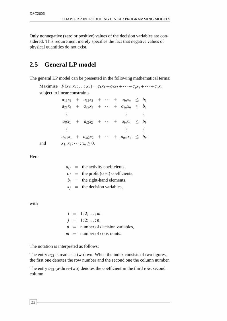
Only nonnegative (zero or positive) values of the decision variables are con-sidered. This requirement merely specifies the fact that negative values ofphysical quantities do not exist.
2.5 General LP model
The general LP model can be presented in the following mathematical terms:
Maximise F(x1; x2; . . . ; xn) = c1x1+c2x2+ · · ·+c jx j + · · ·+cnxn
subject to linear constraints
a11x1 + a12x2 + · · · + alnxn ≤ b1
a21x1 + a22x2 + · · · + a2nxn ≤ b2
......
...
ail x1 + ai2x2 + · · · + ainxn ≤ bi
......
...
am1x1 + am2x2 + · · · + amnxn ≤ bm
and x1; x2; · · · ; xn≥ 0.
Here
ai j = the activity coefficients,
c j = the profit (cost) coefficients,
bi = the right-hand elements,
x j = the decision variables,
with
i = 1; 2; . . . ; m,
j = 1; 2; . . . ; n,
n = number of decision variables,
m = number of constraints.
The notation is interpreted as follows:
The entrya22 is read as a-two-two. When the index consists of two figures,the first one denotes the row number and the second one the column number.
The entrya32 (a-three-two) denotes the coefficient in the third row, secondcolumn.
22
Chapter 3
Graphical representation
Contents3.1 A graphical approach . . . . . . . . . . . . . . . . . . . 24
3.2 Finding the feasible area . . . . . . . . . . . . . . . . . 25
3.3 Identifying the optimal solution . . . . . . . . . . . . . 29
3.4 Solving Christine’s problem graphically . . . . . . . . . 35
3.5 Types of solution . . . . . . . . . . . . . . . . . . . . . . 38
3.5.1 Infeasible LPs . . . . . . . . . . . . . . . . . . . . 38
3.5.2 Unbounded solutions . . . . . . . . . . . . . . . . 38
3.5.3 Multiple optimal solutions . . . . . . . . . . . . . 40
3.5.4 Degenerate solutions . . . . . . . . . . . . . . . . 41
3.6 Types of constraint . . . . . . . . . . . . . . . . . . . . . 42
3.6.1 Redundant constraints . . . . . . . . . . . . . . . 42
3.6.2 Binding and nonbinding constraints . . . . . . . . 42
3.7 Exercises . . . . . . . . . . . . . . . . . . . . . . . . . . 43
3.8 Solutions to exercises . . . . . . . . . . . . . . . . . . . 44
23
DSC2606
CHAPTER 3 GRAPHICAL REPRESENTATION
Sections from prescribed book,WinstonChapter 3, Section 3.1Chapter 3, Section 3.2Chapter 3, Section 3.3
Learning objectivesAfter completing this study unit you should be able to
• use the graphical approach to determine the optimal solution to an LPmodel in two variables
• identify infeasibility, unbounded solutions, multiple solutions and de-generacy from a graph
• identify redundant, binding and nonbinding constraints from a graph.
3.1 A graphical approach
We have now spent a considerable time “transforming” problems into linearprogramming models. We will also spend a considerable time solving themusing a solution method called the simplex method. However,before doingthis, we are going to use a graphical representation of simple LP models toillustrate certain characteristics of LP models. A graphical approach mayalso be used to solve small problems in two decision variables with only afew constraints.
The nonnegativity constraints of linear programming problems restrict thegraphical representation to the first quadrant only. The graphical approachconsists of two phases:
• graphical representation of the feasible area
• identifying the optimal solution.
As an illustration we return to Mark’s problem. This problemwas formu-lated in Section 2.2 as follows:
Maximise PROFIT= 300VH+250SB
subject to
2VH + SB ≤ 40 (Labour time)
VH + 3SB ≤ 45 (Machine time)
VH ≤ 12 (Marketing)
and VH; SB≥ 0.
24
3.2. FINDING THE FEASIBLE AREA
DSC2606
Here
VH = number of sets of modelVH200 produced daily,
SB = number of sets of modelSB150 produced daily.
3.2 Finding the feasible area
The feasible area is established by graphing all of the constraints, whichare in the form of inequalities and/or equations. The two decision variablesunder consideration in Mark’s problem areVH andSB. It does not matterwhich axis is used to represent which variable. We arbitrarily choose thehorizontal axis to representVH.
BothVH andSBare≥ 0. We therefore use only the first quadrant for thegraphical representation. We have to represent the three constraints, whichin this case are inequalities, on the graph. And we start by considering theequality part only(= sign), dropping the less than part(< signs):
2VH + SB = 40 (1)
VH + 3SB = 45 (2)
VH = 12. (3)
In order to draw a line, we need two points. The easiest way to do this is asfollows: set the one variable equal to zero and find the value for the othervariable. This gives a point on one axis. Repeat the process for the othervariable to find a point on the other axis. Connect the points to draw the line.
Consider equation (1): 2VH+SB= 40.
Let VH = 0, thenSB= 40. The point on theSB-axis is(0;40).Let SB= 0, thenVH = 20. The point on theVH-axis is(20;0).
Plot the two points on the axes and draw the line connecting these points.
Consider equation (2):VH+3SB= 45.
Let VH = 0, thenSB= 15. The point on theSB-axis is(0;15).Let SB= 0, thenVH = 45. The point on theVH-axis is(45;0).
Plot the two points on the axes and draw the line.
Consider equation (3):VH = 12.
Any line consisting of one variable only is a line parallel tothe axis repre-senting the other variable. In this case, draw a line parallel to theSB-axis,passing through the point(12;0).
These three lines are drawn and are given in Figure 3.1.
But these lines do not tell us anything about the inequalities.
25

DSC2606
CHAPTER 3 GRAPHICAL REPRESENTATION
5
10
15
20
25
30
35
40
5 10 15 20 25 30 35 40 45 50
SB
VH
2VH+
SB=
40
VH=
12
VH+3SB= 45
Figure 3.1: Equality constraints
Consider the first constraint of Mark’s model, the inequality 2VH+SB≤ 40.
This inequality states that the value of 2VH+SBmust be less than or equalto 40. The equality part(= sign) is easy – all the points on the line 2VH+SB= 40 will satisfy this requirement. To deal with the “less than” part(< sign), we choose any point not on the line. If this point satisfies the in-equality, then all points on the same side of the line will also satisfy theinequality. Conversely, if the point does not satisfy the inequality, then allpoints on the opposite side of the line will satisfy the inequality.
The easiest way to determine on which side of the line the inequality is satis-fied, is to substitute the point(0;0) into the inequality. Then
2VH+SB= 2(0)+0= 0< 40.
The point(0;0) therefore satisfies the inequality and all points on the sameside of the line as(0;0) will satisfy the inequality.
The area satisfying the inequality is represented by the horizontal lines onFigure 3.2.
All the points in the lined area as well as the points on the line 2VH+SB=40 satisfy the inequality 2VH+SB≤ 40. We call this the solution set of theinequality.
NOTE:The equality sign(=) is part of the inequality 2VH+SB≤ 40 andtherefore the line 2VH+SB= 40 is represented by a solid line on the graph.If the inequality was in fact a strict inequality, say 2VH+SB< 40, where theequality sign isnot part of the inequality, then the points on the line 2VH+SB= 40 arenot part of the solution set of the inequality and this fact shouldbe represented on a graph by drawing the line 2VH +SB= 40 as a dottedline.
26
3.2. FINDING THE FEASIBLE AREA
DSC2606
5
10
15
20
25
30
35
40
5 10 15 20 25 30 35 40 45 50
SB
VH
2VH+
SB=
40
VH=
12
VH+3SB= 45
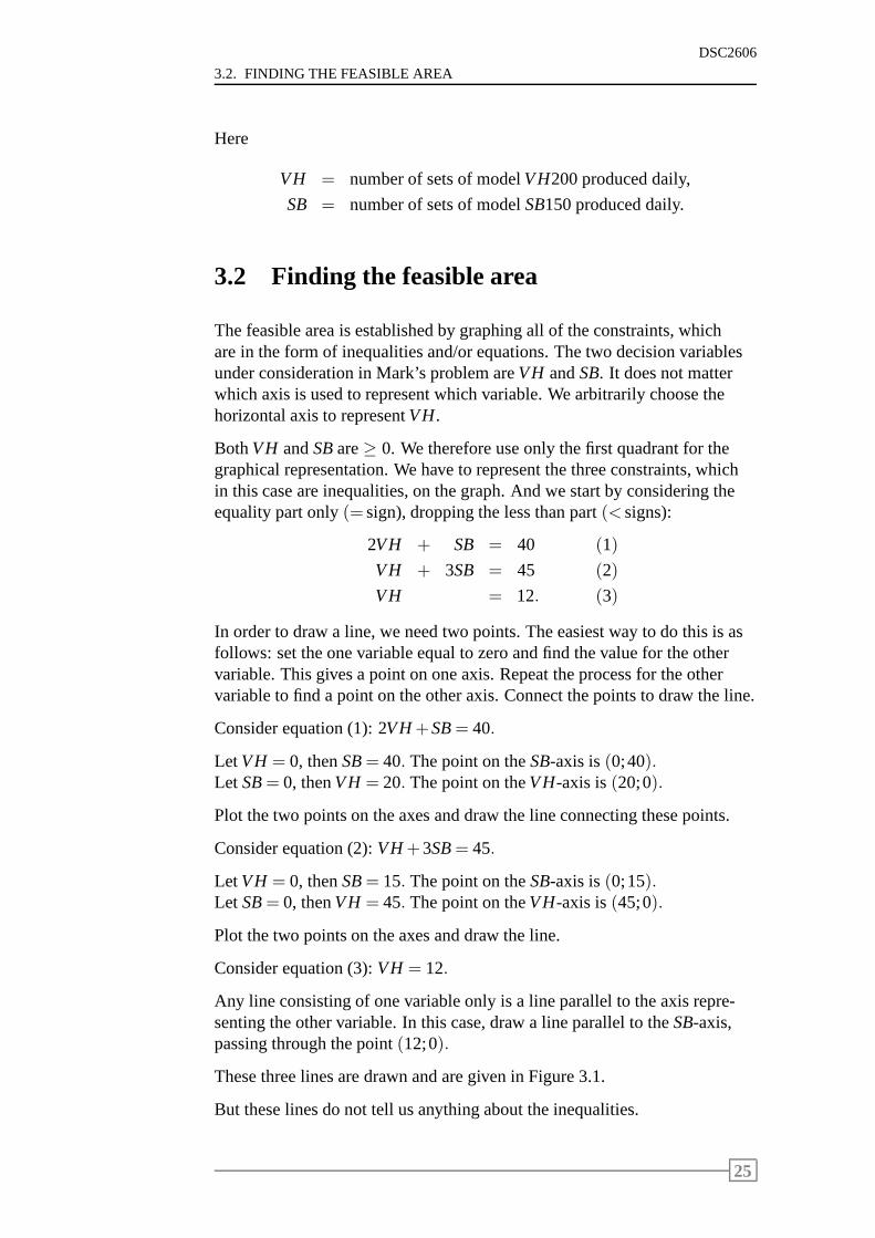
Figure 3.2: Labour time inequality
Now consider the second constraint of Mark’s model,VH+3SB≤ 45, andsubstitute the point(0;0) into this inequality. Then
VH+3SB= 0+3(0) = 0< 45.
The point(0;0) satisfies the inequality and all points on the same side of theline satisfy the inequality.
The solution set of this inequality is represented by the solid lineVH +3SB= 45 and the positively slanted lines on Figure 3.3.
5
10
15
20
25
30
35
40
5 10 15 20 25 30 35 40 45 50
SB
VH
2VH+
SB=
40
VH=
12
VH+3SB= 45
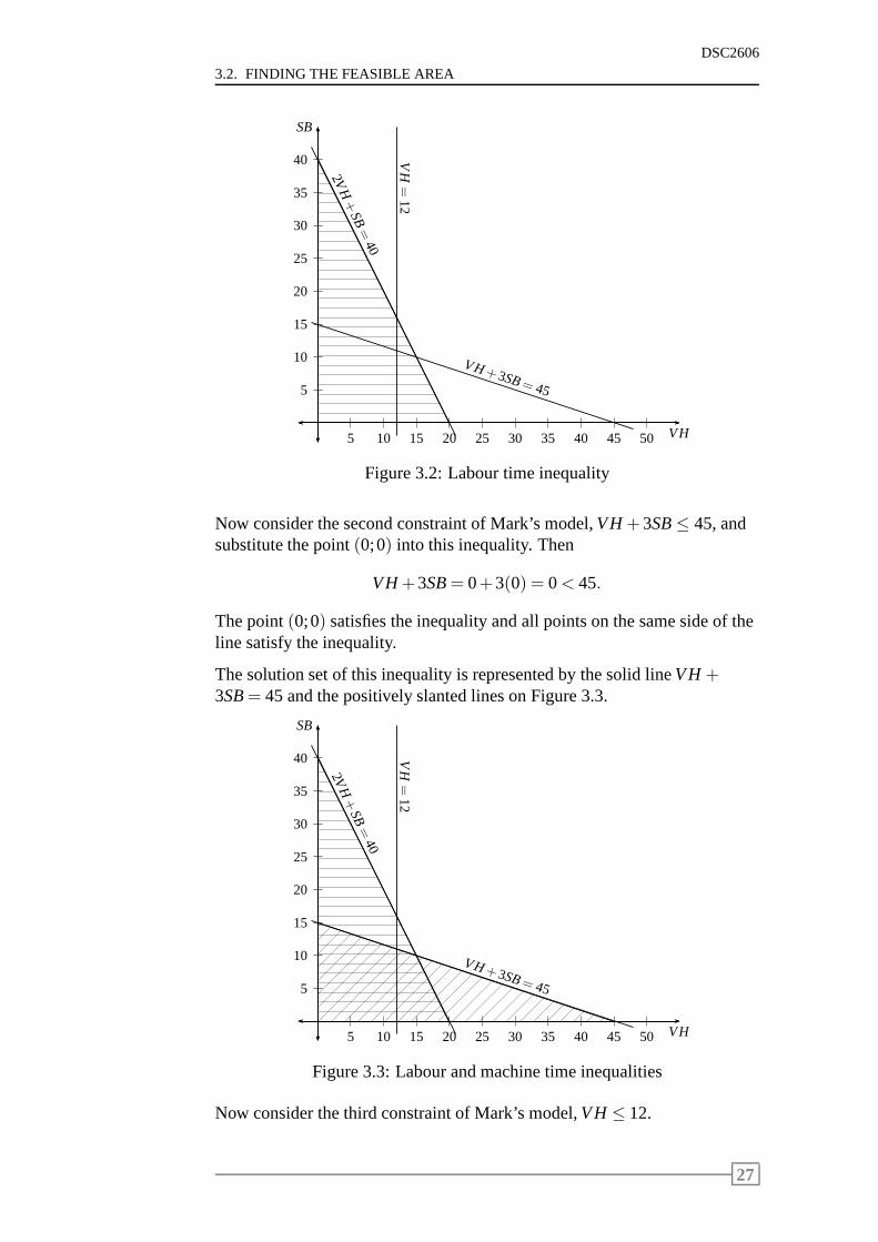
Figure 3.3: Labour and machine time inequalities
Now consider the third constraint of Mark’s model,VH ≤ 12.
27
DSC2606
CHAPTER 3 GRAPHICAL REPRESENTATION
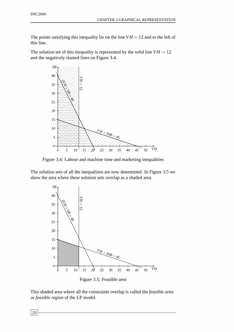
The points satisfying this inequality lie on the lineVH = 12 and to the left ofthis line.
The solution set of this inequality is represented by the solid lineVH = 12and the negatively slanted lines on Figure 3.4.
5
10
15
20
25
30
35
40
5 10 15 20 25 30 35 40 45 50
SB
VH
2VH+
SB=
40
VH=
12
VH+3SB= 45
Figure 3.4: Labour and machine time and marketing inequalities
The solution sets of all the inequalities are now determined. In Figure 3.5 weshow the area where these solution sets overlap as a shaded area.
5
10
15
20
25
30
35
40
5 10 15 20 25 30 35 40 45 50
SB
VH
2VH+
SB=
40
VH=
12
VH+3SB= 45
Figure 3.5: Feasible area
This shaded area where all the constraints overlap is calledthefeasible areaor feasible regionof the LP model.
28
3.3. IDENTIFYING THE OPTIMAL SOLUTION
DSC2606
NOTE:The constraint 2VH+SB≤ 40 makes no contribution to the feasi-ble area, in fact it falls completely outside the feasible area. Any point in thefeasible area will also satisfy this constraint. This “non-contributing” con-straint is called aredundant constraintand can be omitted from the model.
3.3 Identifying the optimal solution
Any point in the feasible area satisfies all the constraints and is thereforea feasible solution to the LP model. Since there are an infinite number ofpoints in this area, there are an infinite number of feasible solutions for thisproblem. To find an optimal solution, it is necessary to identify a solution(point) in the feasible area that maximises the profit (objective function).
How can this be accomplished?
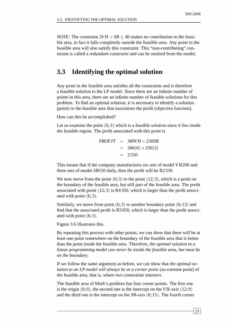
Let us examine the point(6;3) which is a feasible solution since it lies insidethe feasible region. The profit associated with this point is
PROFIT = 300VH+250SB
= 300(6)+250(3)
= 2550.
This means that if the company manufactures six sets of modelVH200 andthree sets of modelSB150 daily, then the profit will be R2550.
We now move from the point(6;3) to the point(12;3), which is a point onthe boundary of the feasible area, but still part of the feasible area. The profitassociated with point(12;3) is R4350, which is larger than the profit associ-ated with point(6;3).
Similarly, we move from point(6;3) to another boundary point(6;13) andfind that the associated profit is R5050, which is larger than the profit associ-ated with point(6;3).
Figure 3.6 illustrates this.
By repeating this process with other points, we can show thatthere will be atleast one point somewhere on the boundary of the feasible area that is betterthan the point inside the feasible area. Therefore,the optimal solution to alinear programming model can never be inside the feasible area, but must beon the boundary.
If we follow the same argument as before, we can show thatthe optimal so-lution to an LP model will always be at a corner point(an extreme point) ofthe feasible area, that is, where two constraints intersect.
The feasible area of Mark’s problem has four corner points. The first oneis the origin(0;0), the second one is the intercept on theVH-axis(12;0)and the third one is the intercept on theSB-axis(0;15). The fourth corner
29
DSC2606
CHAPTER 3 GRAPHICAL REPRESENTATION
5
10
15
20
25
30
5 10 15 20 25 30 35 40 45
SB
VH
VH=
12
VH+3SB= 45b
b
b
(6;13)PROFIT= 5050
(6;3)PROFIT= 2550
(12;3)PROFIT= 4350
Figure 3.6: Searching for the optimal solution
point is at the intersection of the two constraints. If we substituteVH = 12in VH+3SB= 45, we obtainSB= 11. The fourth corner point is(12;11).
Let us calculate the value of the objective function at the corner points of thefeasible region:
Corner points Value of objective function(VH;SB) PROFIT= 300VH+250SB(0;0) 0(12;0) 3 600(12;11) 6 350(0;15) 3 750
From this we see that the point(12;11) gives the maximum profit. There-fore, the optimal solution is to produce 12 sets of modelVH200 and 11 setsof modelSB150 for a profit of R6350.
This method of calculating the value of the objective function at the cornerpoints is not very efficient and may be a very lengthy exercise.
A more efficient method for obtaining the optimal solution must be found.The optimal solution is the solution thatoptimises(maximises in this case)the objective function. Therefore, it is obvious that we should use the objec-tive function to find the optimal solution.
The objective function of Mark’s problem is
MaximumPROFIT= 300VH+250SB.
30
3.3. IDENTIFYING THE OPTIMAL SOLUTION
DSC2606
Let us examine a point, say(5;5) in the feasible area. Here five units of eachtype of model are produced and the associated profit is
PROFIT= 300(5)+250(5) = 2750.
The objective function can now be written as
300VH+250SB= 2750.
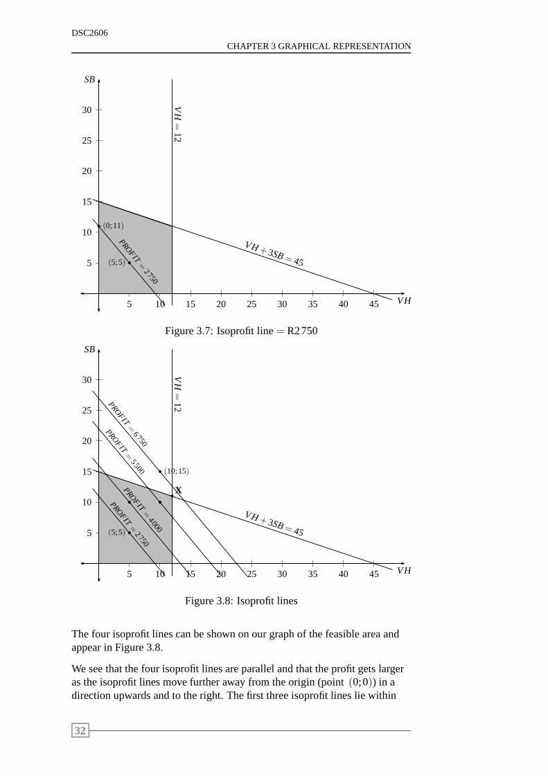
This is the equation of a straight line and each of the points on this line willhave an objective function value (profit) of R2750. This lineis called anisoprofit line because all points on it have the same profit(in Greek “iso”means “same”).
We now want to draw this line and we proceed as follows:
We already have one point, namely(5;5). To find another point, we calcu-late the intercept on theSB-axis. IfVH = 0 then
300VH+250SB = 2750
300(0)+250SB = 2750
SB = 11.
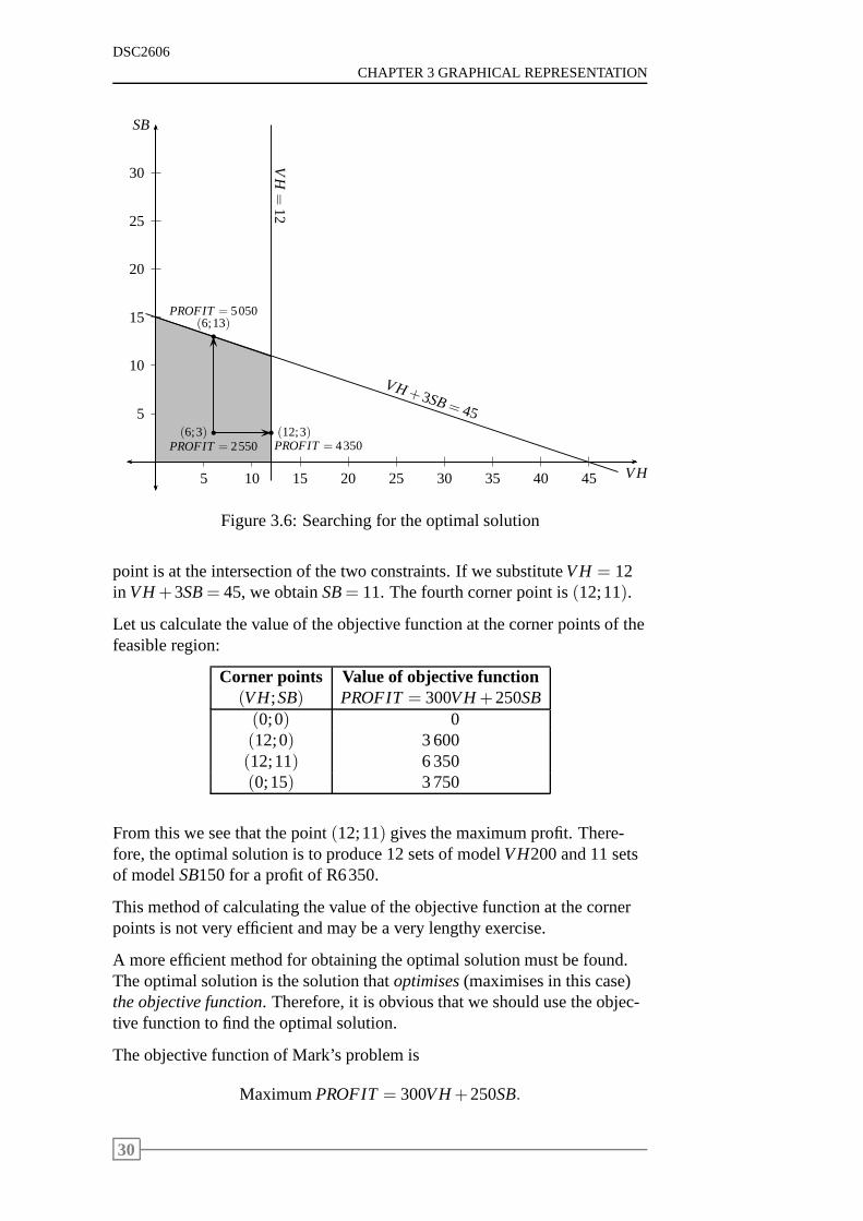
We can use the points(5;5) and(0;11) to draw the isoprofit line
300VH+250SB= 2750.
And this is shown in Figure 3.7 by the dashed line. We use a dashed line sothat we can distinguish the isoprofit line from the constraints.
Choose another point in the feasible region, say(5;10). An isoprofit linegoing through this point will have a corresponding profit of
PROFIT= 300(5)+250(10) = 4000.
TheSB-intercept of 300VH+250SB= 4000 is atVH = 0, and isSB= 16.
We can use the points(5;10) and(0;16) to draw the isoprofit line
300VH+250SB= 4000.
Likewise, points(10;10) and(0;22) can be used to draw the isoprofit line
300VH+250SB= 5500.
And points(10;15) and(0;27) can be used to draw the isoprofit line
300VH+250SB= 6750.
31
DSC2606
CHAPTER 3 GRAPHICAL REPRESENTATION
5
10
15
20
25
30
5 10 15 20 25 30 35 40 45
SB
VH
VH=
12
VH+3SB= 45b
b
(5;5)
(0;11)
PROFIT
=2750
Figure 3.7: Isoprofit line= R2750
5
10
15
20
25
30
5 10 15 20 25 30 35 40 45
SB
VH
VH=
12
VH+3SB= 45
PROFIT
=2750
PROFIT
=4000
PROFIT
=5500
PROFIT
=6750
b
b b
b
b
(5;5)
(10;15)
X
Figure 3.8: Isoprofit lines
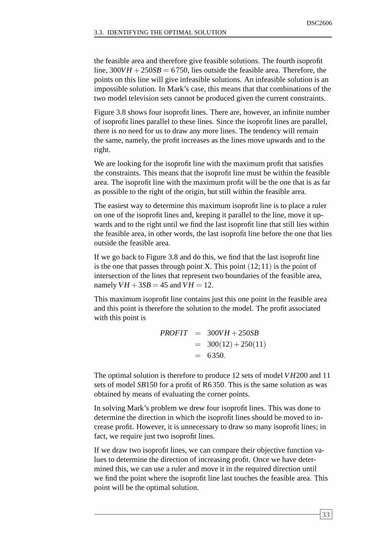
The four isoprofit lines can be shown on our graph of the feasible area andappear in Figure 3.8.
We see that the four isoprofit lines are parallel and that the profit gets largeras the isoprofit lines move further away from the origin (point (0;0)) in adirection upwards and to the right. The first three isoprofit lines lie within
32
3.3. IDENTIFYING THE OPTIMAL SOLUTION
DSC2606
the feasible area and therefore give feasible solutions. The fourth isoprofitline, 300VH+250SB= 6750, lies outside the feasible area. Therefore, thepoints on this line will give infeasible solutions. An infeasible solution is animpossible solution. In Mark’s case, this means that that combinations of thetwo model television sets cannot be produced given the current constraints.
Figure 3.8 shows four isoprofit lines. There are, however, aninfinite numberof isoprofit lines parallel to these lines. Since the isoprofit lines are parallel,there is no need for us to draw any more lines. The tendency will remainthe same, namely, the profit increases as the lines move upwards and to theright.
We are looking for the isoprofit line with the maximum profit that satisfiesthe constraints. This means that the isoprofit line must be within the feasiblearea. The isoprofit line with the maximum profit will be the onethat is as faras possible to the right of the origin, but still within the feasible area.
The easiest way to determine this maximum isoprofit line is toplace a ruleron one of the isoprofit lines and, keeping it parallel to the line, move it up-wards and to the right until we find the last isoprofit line thatstill lies withinthe feasible area, in other words, the last isoprofit line before the one that liesoutside the feasible area.
If we go back to Figure 3.8 and do this, we find that the last isoprofit lineis the one that passes through point X. This point(12;11) is the point ofintersection of the lines that represent two boundaries of the feasible area,namelyVH+3SB= 45 andVH = 12.
This maximum isoprofit line contains just this one point in the feasible areaand this point is therefore the solution to the model. The profit associatedwith this point is
PROFIT = 300VH+250SB
= 300(12)+250(11)
= 6350.
The optimal solution is therefore to produce 12 sets of modelVH200 and 11sets of modelSB150 for a profit of R6350. This is the same solution as wasobtained by means of evaluating the corner points.
In solving Mark’s problem we drew four isoprofit lines. This was done todetermine the direction in which the isoprofit lines should be moved to in-crease profit. However, it is unnecessary to draw so many isoprofit lines; infact, we require just two isoprofit lines.
If we draw two isoprofit lines, we can compare their objectivefunction va-lues to determine the direction of increasing profit. Once wehave deter-mined this, we can use a ruler and move it in the required direction untilwe find the point where the isoprofit line last touches the feasible area. Thispoint will be the optimal solution.
33
DSC2606
CHAPTER 3 GRAPHICAL REPRESENTATION
The fact that the isoprofit lines are parallel, and thereforehave the sameslope, can be applied to derive yet another method of drawingthe isoprofitlines.
The objective function can be rewritten as follows:
300VH+250SB = PROFIT
250SB = −300VH+PROFIT
SB = −300250
VH+PROFIT
250
SB = −65VH+
PROFIT250
.
(The function is rewritten by writingSBin terms ofVH andPROFIT sinceSBis represented on the vertical axis of the graph.)
The slope of all the isoprofit lines will then be−65. The slope is negative,
which means that the slant is\, in contrast to a positive slope which hasslant/.
To draw the first isoprofit line, we measure six units on the vertical axis andfive units on the horizontal axis and draw a line through thesepoints. Inother words, we draw a line through points(0;6) and(5;0).
To determine the value of this isoprofit line, we substitute either of thesepoints into the objective function. Then
PROFIT = 300VH+250SB
= 300(0)+250(6)
= 1500.
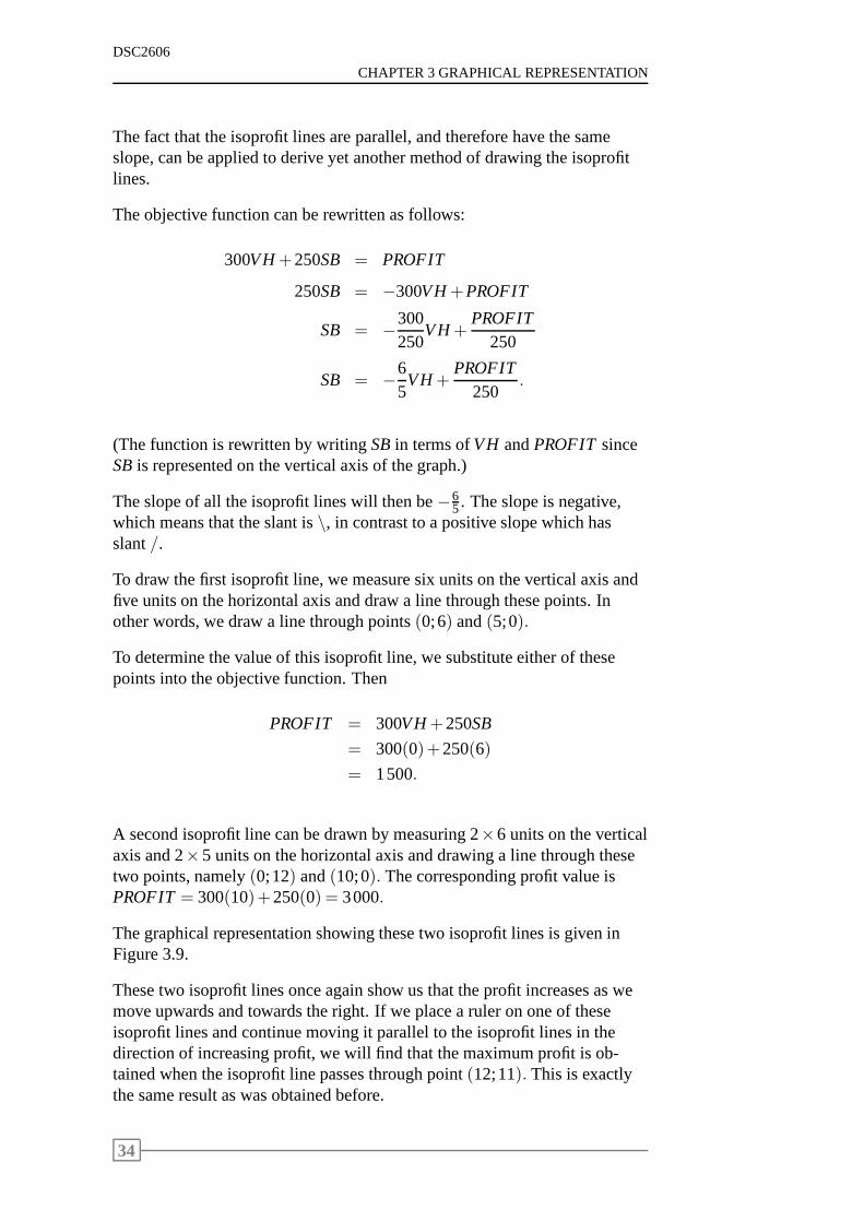
A second isoprofit line can be drawn by measuring 2×6 units on the verticalaxis and 2×5 units on the horizontal axis and drawing a line through thesetwo points, namely(0;12) and(10;0). The corresponding profit value isPROFIT= 300(10)+250(0) = 3000.
The graphical representation showing these two isoprofit lines is given inFigure 3.9.
These two isoprofit lines once again show us that the profit increases as wemove upwards and towards the right. If we place a ruler on one of theseisoprofit lines and continue moving it parallel to the isoprofit lines in thedirection of increasing profit, we will find that the maximum profit is ob-tained when the isoprofit line passes through point(12;11). This is exactlythe same result as was obtained before.
34
3.4. SOLVING CHRISTINE’S PROBLEM GRAPHICALLY
DSC2606
5
10
15
20
25
30
5 10 15 20 25 30 35 40 45
SB
VHV
H=
12
VH+3SB= 45
PROFIT
=1500
PROFIT
=3000
b(12;11)
Figure 3.9: Two isoprofit lines
3.4 Solving Christine’s problem graphically
The graphical approach can also be used for minimisation problems. As anillustration, we return to Christine’s LP model (see Section 2.3):
Minimise COST= 45ALPHA+12BETA
subject to
ALPHA + BETA ≥ 300 (Brilliance)
3ALPHA ≥ 250 (Tint)
and ALPHA; BETA≥ 0.
Here
ALPHA = quantity (in grams) of Alpha in each tin of paint,
BETA = quantity (in grams) of Beta in each tin of paint.
The cost is given in cents per gram.
Let us decide thatALPHAwill be represented on the horizontal axis andBETAon the vertical axis.
The first constraint is rewritten as an equality as
ALPHA+BETA= 300.
Let ALPHA= 0, thenBETA= 300. The point on theBETA-axis is(0;300).
35
DSC2606
CHAPTER 3 GRAPHICAL REPRESENTATION
Let BETA=0, thenALPHA=300. The point on theALPHA-axis is(300;0).
Plot these two points on the axes and draw the line connectingthem.
Now substitute point(0;0) into the constraint. Then
ALPHA+BETA ≥ 300
0+0 � 300.
The point(0;0) does not satisfy the inequality and so(0;0) is not part of thefeasible area. All points on the opposite side of the lineALPHA+BETA=300 will satisfy the inequality.
Now rewrite the second constraint as an equation. Then
3ALPHA = 250
ALPHA = 83,33.
This line is a straight line parallel to theBETA-axis, passing through thepoint (83,33;0).
The point(0;0) does not satisfy the inequality 3ALPHA≥ 250 and thereforeit does not form part of the feasible area.
The objective function is now rewritten as
COST = 45ALPHA+12BETA
12BETA = −45ALPHA+COST
BETA = −4512
ALPHA+COST
12
= −154
ALPHA+COST
12.
The slope of the isocost lines is−154 .
We can draw the first isocost line by measuring say 10× 15= 150 unitson the vertical axis and 10× 4 = 40 units on the horizontal axis, and thendrawing a line through these points(0;150) and(40;0).
The cost associated with this isocost line is
COST = 45ALPHA+12BETA
= 45(40)+12(0)
= 1800.
A second isocost line can be drawn by measuring 30×15= 450 units on thevertical axis and 30×4 = 120 units on the horizontal axis, and then draw-ing a line through these points(0;450) and(120;0). The associated cost isR5400.
36
3.4. SOLVING CHRISTINE’S PROBLEM GRAPHICALLY
DSC2606
50
100
150
200
250
300
350
400
450
500
50 100 150 200 250 300 350ALPHA
BETA
ALPHA+
BETA=300
3ALP
HA=
25
0
CO
ST=
1800
CO
ST=
5400
b A
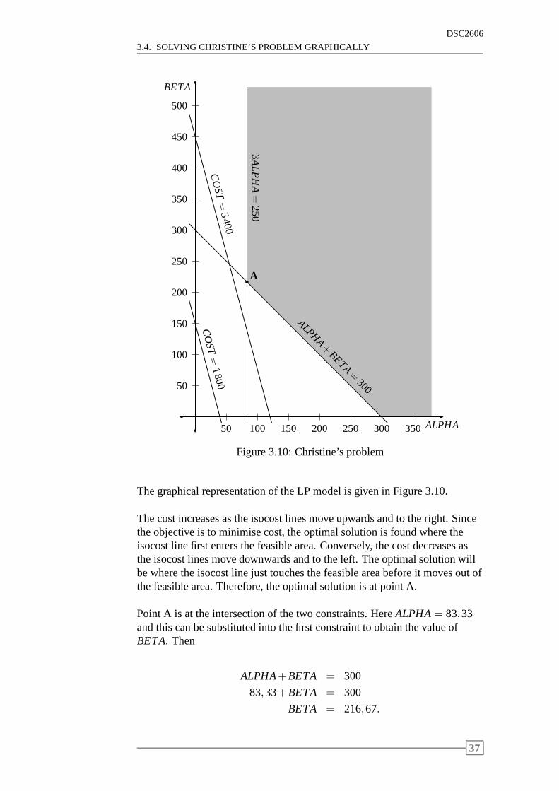
Figure 3.10: Christine’s problem
The graphical representation of the LP model is given in Figure 3.10.
The cost increases as the isocost lines move upwards and to the right. Sincethe objective is to minimise cost, the optimal solution is found where theisocost line first enters the feasible area. Conversely, thecost decreases asthe isocost lines move downwards and to the left. The optimalsolution willbe where the isocost line just touches the feasible area before it moves out ofthe feasible area. Therefore, the optimal solution is at point A.
Point A is at the intersection of the two constraints. HereALPHA= 83,33and this can be substituted into the first constraint to obtain the value ofBETA. Then
ALPHA+BETA = 300
83,33+BETA = 300
BETA = 216,67.
37
DSC2606
CHAPTER 3 GRAPHICAL REPRESENTATION
The optimal solution to Christine’s problem is to use 83,33 grams of Alphaand 216,67 grams of Beta in each tin of paint.
The minimum cost will be
COST = 45ALPHA+12BETA
= 45(83,33)+12(216,67)
= 6350.
The cost is given in cents and therefore the minimum cost is R63,50 per tinof paint.
3.5 Types of solution
We have now solved Mark and Christine’s problems by means of the graph-ical approach. And each of these models had a single optimal solution. Thismay not always be the case. It may happen that an LP model has nosolu-tion, or even has many optimal solutions. Let us consider thedifferent typesof solution that can be obtained for LP models.
3.5.1 Infeasible LPs
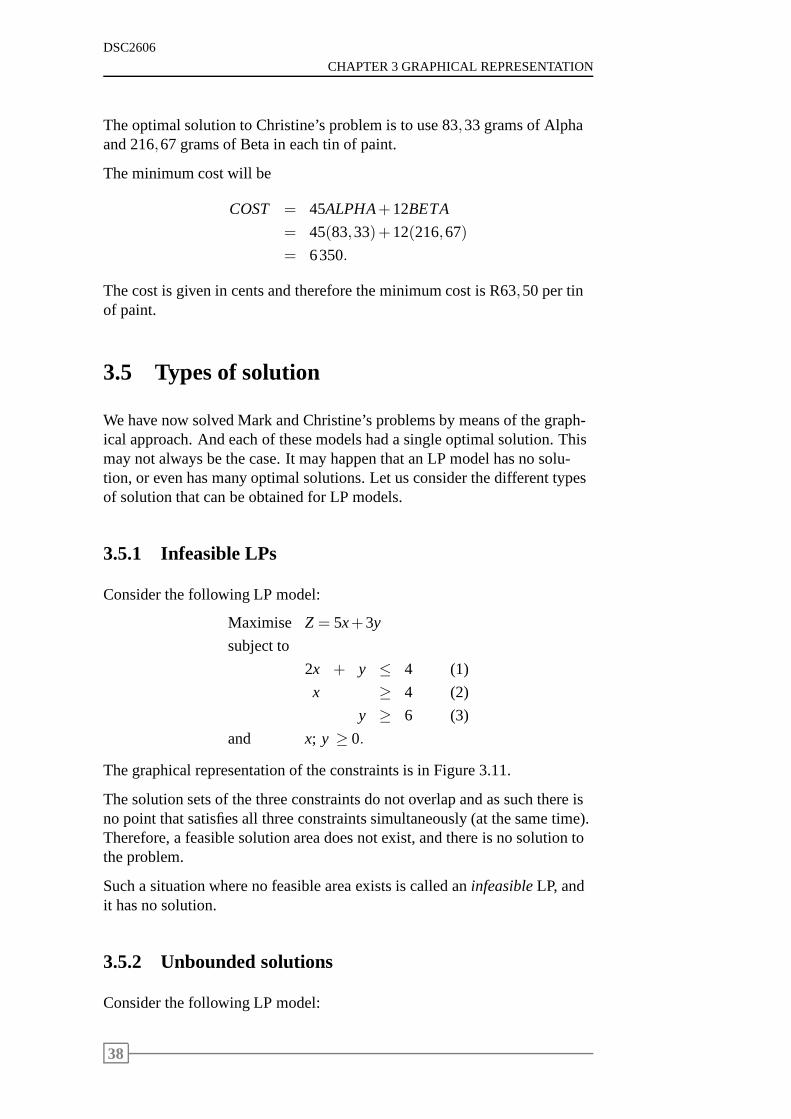
Consider the following LP model:
Maximise Z = 5x+3y
subject to
2x + y ≤ 4 (1)
x ≥ 4 (2)
y ≥ 6 (3)
and x; y ≥ 0.
The graphical representation of the constraints is in Figure 3.11.
The solution sets of the three constraints do not overlap andas such there isno point that satisfies all three constraints simultaneously (at the same time).Therefore, a feasible solution area does not exist, and there is no solution tothe problem.
Such a situation where no feasible area exists is called aninfeasibleLP, andit has no solution.
3.5.2 Unbounded solutions
Consider the following LP model:
38
3.5. TYPES OF SOLUTION
DSC2606
2
4
6
8
2 4 6 8x
y
(1)
(2)
(3)
Figure 3.11: Infeasible LP
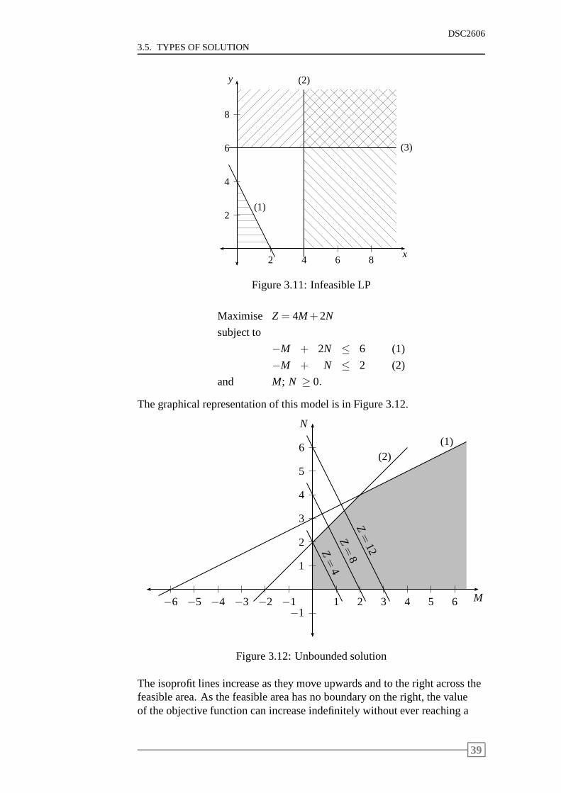
Maximise Z = 4M+2N
subject to
−M + 2N ≤ 6 (1)
−M + N ≤ 2 (2)
and M; N ≥ 0.
The graphical representation of this model is in Figure 3.12.
1
2
3
4
5
6
−11 2 3 4 5 6−1−2−3−4−5−6 M
N
(1)(2)
Z=
4Z=
8Z=
12
Figure 3.12: Unbounded solution
The isoprofit lines increase as they move upwards and to the right across thefeasible area. As the feasible area has no boundary on the right, the valueof the objective function can increase indefinitely withoutever reaching a
39
DSC2606
CHAPTER 3 GRAPHICAL REPRESENTATION
maximum.
This LP model is said to have anunbounded solution.
3.5.3 Multiple optimal solutions
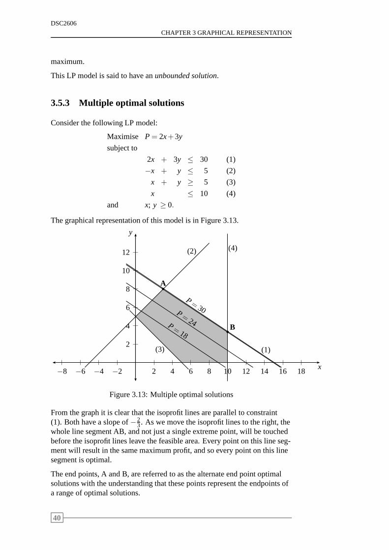
Consider the following LP model:
Maximise P= 2x+3y
subject to
2x + 3y ≤ 30 (1)
−x + y ≤ 5 (2)
x + y ≥ 5 (3)
x ≤ 10 (4)
and x; y ≥ 0.
The graphical representation of this model is in Figure 3.13.
2
4
6
8
10
12
2 4 6 8 10 12 14 16 18−2−4−6−8x
y
(1)
(2)
(3)
(4)
b
b
B
A
P= 18
P= 24
P= 30
Figure 3.13: Multiple optimal solutions
From the graph it is clear that the isoprofit lines are parallel to constraint(1). Both have a slope of−2
3. As we move the isoprofit lines to the right, thewhole line segment AB, and not just a single extreme point, will be touchedbefore the isoprofit lines leave the feasible area. Every point on this line seg-ment will result in the same maximum profit, and so every pointon this linesegment is optimal.
The end points, A and B, are referred to as the alternate end point optimalsolutions with the understanding that these points represent the endpoints ofa range of optimal solutions.
40
3.5. TYPES OF SOLUTION
DSC2606
This LP model is said to havemultiple optimal solutions.
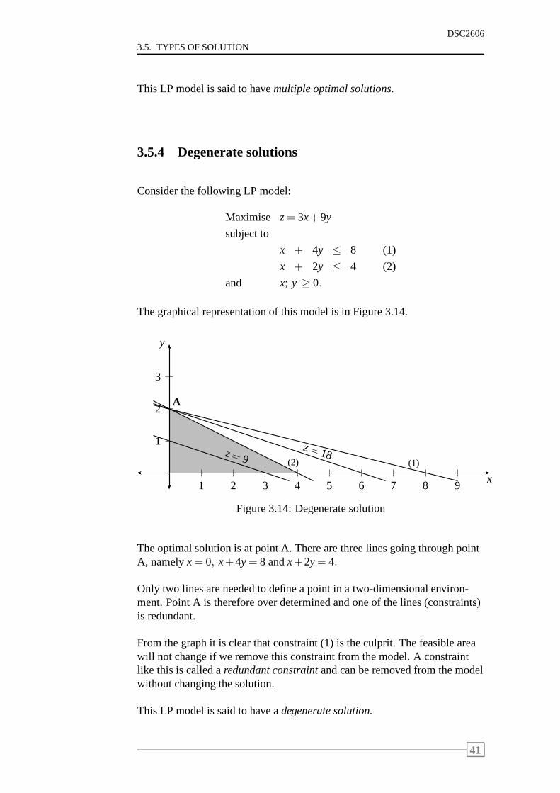
3.5.4 Degenerate solutions
Consider the following LP model:
Maximise z= 3x+9y
subject to
x + 4y ≤ 8 (1)
x + 2y ≤ 4 (2)
and x; y ≥ 0.
The graphical representation of this model is in Figure 3.14.
1
2
3
1 2 3 4 5 6 7 8 9x
y
(1)(2)
A
z= 9z= 18
Figure 3.14: Degenerate solution
The optimal solution is at point A. There are three lines going through pointA, namelyx= 0, x+4y= 8 andx+2y= 4.
Only two lines are needed to define a point in a two-dimensional environ-ment. Point A is therefore over determined and one of the lines (constraints)is redundant.
From the graph it is clear that constraint (1) is the culprit.The feasible areawill not change if we remove this constraint from the model. Aconstraintlike this is called aredundant constraintand can be removed from the modelwithout changing the solution.
This LP model is said to have adegenerate solution.
41
DSC2606
CHAPTER 3 GRAPHICAL REPRESENTATION
3.6 Types of constraint
3.6.1 Redundant constraints
Let us refer back to Mark’s problem. The labour time constraint, 2VH +SB≤ 40, falls outside the feasible area and makes no contribution tothefeasible area. Therefore, it is aredundantconstraint.
The redundant constraint can be removed from the model. In fact, it shouldbe removed, since it only complicates the model and does not make any pos-itive contribution.
3.6.2 Binding and nonbinding constraints
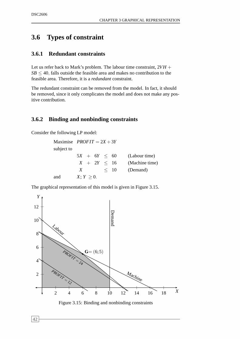
Consider the following LP model:
Maximise PROFIT= 2X+3Y
subject to
5X + 6Y ≤ 60 (Labour time)
X + 2Y ≤ 16 (Machine time)
X ≤ 10 (Demand)
and X; Y ≥ 0.
The graphical representation of this model is given in Figure 3.15.
2
4
6
8
10
12
2 4 6 8 10 12 14 16 18 X
Y
Labour
Machine
Dem
and
b G= (6;5)
PROFIT= 12
PROFIT= 24
Figure 3.15: Binding and nonbinding constraints
42
3.7. EXERCISES
DSC2606
The optimal solution is found at point G where the labour timeand machinetime constraints intersect, that is, whereX = 6 andY = 5.
We now substitute these optimal values into the constraints.
If we substituteX = 6 andY = 5 into the labour time constraint, we find
left-hand side = 5X+6Y
= 5(6)+6(5)
= 60
= right-hand side.
Likewise the left-hand side of the machine time constraint equals the right-hand side at the optimal point(X;Y) = (6;5).
This means that the available labour time and machine time are completelyused up. Constraints like these where the resources are fully utilised arecalledbinding constraints.
We now substitute the optimal values into the demand constraint and find
left-hand side= X = 6< 10= right-hand side.
From this we see that the optimal quantity ofX produced is less than themaximum number demanded, that is, it is not optimal to produce the maxi-mum number demanded.
The difference between the left-hand side and the right-hand side of a con-straint is called thesurplusor slack, depending on the context of the prob-lem.
A constraint where the resource is not utilised fully, in other words, wherethere is surplus or slack, is called anonbinding constraint.
From the graph we see that a constraint is binding if the optimal solutionfalls on the line representing the constraint and a constraint is nonbinding ifthe optimal solution does not fall on the line representing the constraint.
3.7 Exercises
1. Holiday Meal Turkey Ranch buys two different brands of turkey feedand blends them to provide a good, low-cost diet for its turkeys. Eachbrand of feed contains some or all of the three nutritional ingredientsessential for fattening turkeys. Each kilogram of brand 1 contains 6grams of ingredient A, 4 grams of ingredient B and 0,5 grams of in-gredient C. Each kilogram of brand 2 contains 9 grams of ingredientA, 3 grams of ingredient B, but nothing of ingredient C. The brand 1feed costs the Ranch 75c a kilogram, while the brand 2 feed costs R1 akilogram.
43
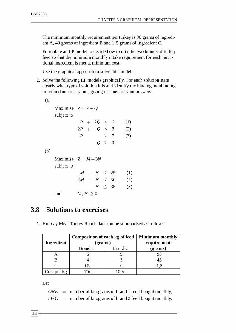
DSC2606
CHAPTER 3 GRAPHICAL REPRESENTATION
The minimum monthly requirement per turkey is 90 grams of ingredi-ent A, 48 grams of ingredient B and 1,5 grams of ingredient C.
Formulate an LP model to decide how to mix the two brands of turkeyfeed so that the minimum monthly intake requirement for eachnutri-tional ingredient is met at minimum cost.
Use the graphical approach to solve this model.
2. Solve the following LP models graphically. For each solution stateclearly what type of solution it is and identify the binding,nonbindingor redundant constraints, giving reasons for your answers.
(a)
Maximise Z = P+Q
subject to
P + 2Q ≤ 6 (1)
2P + Q ≤ 8 (2)
P ≥ 7 (3)
Q ≥ 0.
(b)
Maximise Z = M+3N
subject to
M + N ≤ 25 (1)
2M + N ≤ 30 (2)
N ≤ 35 (3)
and M; N ≥ 0.
3.8 Solutions to exercises
1. Holiday Meal Turkey Ranch data can be summarised as follows:
Composition of each kg of feed Minimum monthlyIngredient (grams) requirement
Brand 1 Brand 2 (grams)A 6 9 90B 4 3 48C 0,5 0 1,5
Cost per kg 75c 100c
Let
ONE = number of kilograms of brand 1 feed bought monthly,
TWO = number of kilograms of brand 2 feed bought monthly.
44
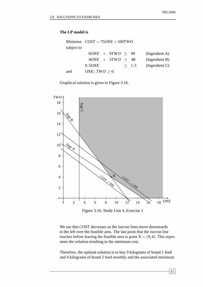
3.8. SOLUTIONS TO EXERCISES
DSC2606
The LP model is
Minimise COST= 75ONE+100TWO
subject to
6ONE + 9TWO ≥ 90 (Ingredient A)
4ONE + 3TWO ≥ 48 (Ingredient B)
0,5ONE ≥ 1,5 (Ingredient C)
and ONE; TWO≥ 0.
Graphical solution is given in Figure 3.16.
2
4
6
8
10
12
14
16
18
2 4 6 8 10 12 14 16 18ONE
TWO
Ingr A
Ingr B
Ing
rC
b XCOST=900
COST=1200
Figure 3.16: Study Unit 4, Exercise 1
We see thatCOSTdecreases as the isocost lines move downwardsto the left over the feasible area. The last point that the isocost linetouches before leaving the feasible area is point X= (9;4). This repre-sents the solution resulting in the minimum cost.
Therefore, the optimal solution is to buy 9 kilograms of brand 1 feedand 4 kilograms of brand 2 feed monthly and the associated minimum
45

DSC2606
CHAPTER 3 GRAPHICAL REPRESENTATION
cost per turkey is
COST = 75ONE+100TWO
= 75(9)+100(4)
= 1075
= R10,75.
2. (a) The graphical representation of the constraints is given in Figure3.17.
1
2
3
4
5
6
7
8
1 2 3 4 5 6 7 8 9 10 P
Q
(1)
(2)
(3)
Figure 3.17: Study Unit 4, Exercise 2(a)
There is no area satisfying all the inequalities simultaneously andso no feasible area exists. We say the LP model (or the problem)is infeasible. There is no solution to this LP model.
(b) The graphical solution to the LP model is given in Figure 3.18.
We see that the objective function valueZ increases as the iso-profit lines are moved upwards and to the right across the fea-sible region. The last point where an isoprofit line touches thefeasible area before moving out of the feasible area is at point K= (0;25), and this is the optimal solution.
The optimal solution is atM = 0 andN = 25 and the associatedmaximum value of the objective function is
Z = M+3N
= 0+3(25)
= 75.
46
3.8. SOLUTIONS TO EXERCISES
DSC2606
5
10
15
20
25
30
35
5 10 15 20 25 30 35 M
N
(1)(2)
(3)
K
Z = 15
Z = 30
MaximumZ-value
Figure 3.18: Study Unit 4, Exercise 2(b)
The optimal solution lies on constraint (1) and so it is a bindingconstraint.
The optimal solution does not lie on constraint (2) and so it is anonbinding constraint.
Constraint (3) does not influence the feasible area and so it is aredundant constraint.
47

DSC2606
CHAPTER 3 GRAPHICAL REPRESENTATION
48
Chapter 4
Computer solutions
Contents4.1 Introduction . . . . . . . . . . . . . . . . . . . . . . . . 50
4.2 Using LINGO . . . . . . . . . . . . . . . . . . . . . . . 50
4.3 Solving Mark’s problem with LINGO . . . . . . . . . . 51
4.4 Solving Christine’s problem with LINGO . . . . . . . . 53
4.5 Exercises . . . . . . . . . . . . . . . . . . . . . . . . . . 54
4.6 Solutions to exercises . . . . . . . . . . . . . . . . . . . 54
49
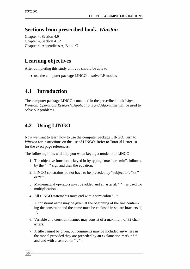
DSC2606
CHAPTER 4 COMPUTER SOLUTIONS
Sections from prescribed book,WinstonChapter 4, Section 4.9Chapter 4, Section 4.12Chapter 4, Appendices A, B and C
Learning objectivesAfter completing this study unit you should be able to
• use the computer package LINGO to solve LP models
4.1 Introduction
The computer package LINGO, contained in the prescribed book WayneWinston: Operations Research, Applications and Algorithmswill be used tosolve our problems.
4.2 Using LINGO
Now we want to learn how to use the computer package LINGO. Turn toWinstonfor instructions on the use of LINGO. Refer to Tutorial Letter 101for the exact page references.
The following hints will help you when keying a model into LINGO:
1. The objective function is keyed in by typing “max” or “min”, followedby the “=” sign and then the equation.
2. LINGO constraints do not have to be preceded by “subject to”, “s.t.”or “st”.
3. Mathematical operators must be added and an asterisk “ * ” is used formultiplication.
4. All LINGO statements must end with a semicolon “ ; ”.
5. A constraint name may be given at the beginning of the line contain-ing the constraint and the name must be enclosed in square brackets “[]”.
6. Variable and constraint names may consist of a maximum of 32 char-acters.
7. A title cannot be given, but comments may be included anywhere inthe model provided they are preceded by an exclamation mark “! ”and end with a semicolon “ ; ”.
50
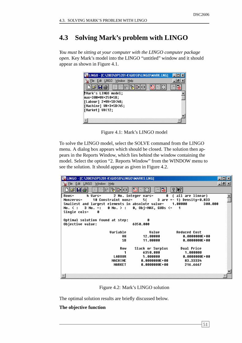
4.3. SOLVING MARK’S PROBLEM WITH LINGO
DSC2606
4.3 Solving Mark’s problem with LINGO
You must be sitting at your computer with the LINGO computer packageopen. Key Mark’s model into the LINGO “untitled” window and it shouldappear as shown in Figure 4.1.
Figure 4.1: Mark’s LINGO model
To solve the LINGO model, select the SOLVE command from the LINGOmenu. A dialog box appears which should be closed. The solution then ap-pears in the Reports Window, which lies behind the window containing themodel. Select the option “2. Reports Window” from the WINDOWmenu tosee the solution. It should appear as given in Figure 4.2.
Figure 4.2: Mark’s LINGO solution
The optimal solution results are briefly discussed below.
The objective function
51
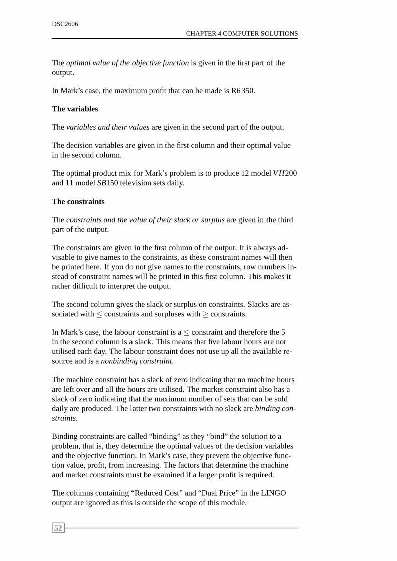
DSC2606
CHAPTER 4 COMPUTER SOLUTIONS
Theoptimal value of the objective functionis given in the first part of theoutput.
In Mark’s case, the maximum profit that can be made is R6350.
The variables
Thevariables and their valuesare given in the second part of the output.
The decision variables are given in the first column and theiroptimal valuein the second column.
The optimal product mix for Mark’s problem is to produce 12 modelVH200and 11 modelSB150 television sets daily.
The constraints
Theconstraints and the value of their slack or surplusare given in the thirdpart of the output.
The constraints are given in the first column of the output. Itis always ad-visable to give names to the constraints, as these constraint names will thenbe printed here. If you do not give names to the constraints, row numbers in-stead of constraint names will be printed in this first column. This makes itrather difficult to interpret the output.
The second column gives the slack or surplus on constraints.Slacks are as-sociated with≤ constraints and surpluses with≥ constraints.
In Mark’s case, the labour constraint is a≤ constraint and therefore the 5in the second column is a slack. This means that five labour hours are notutilised each day. The labour constraint does not use up all the available re-source and is anonbinding constraint.
The machine constraint has a slack of zero indicating that nomachine hoursare left over and all the hours are utilised. The market constraint also has aslack of zero indicating that the maximum number of sets thatcan be solddaily are produced. The latter two constraints with no slackarebinding con-straints.
Binding constraints are called “binding” as they “bind” thesolution to aproblem, that is, they determine the optimal values of the decision variablesand the objective function. In Mark’s case, they prevent theobjective func-tion value, profit, from increasing. The factors that determine the machineand market constraints must be examined if a larger profit is required.
The columns containing “Reduced Cost” and “Dual Price” in the LINGOoutput are ignored as this is outside the scope of this module.
52
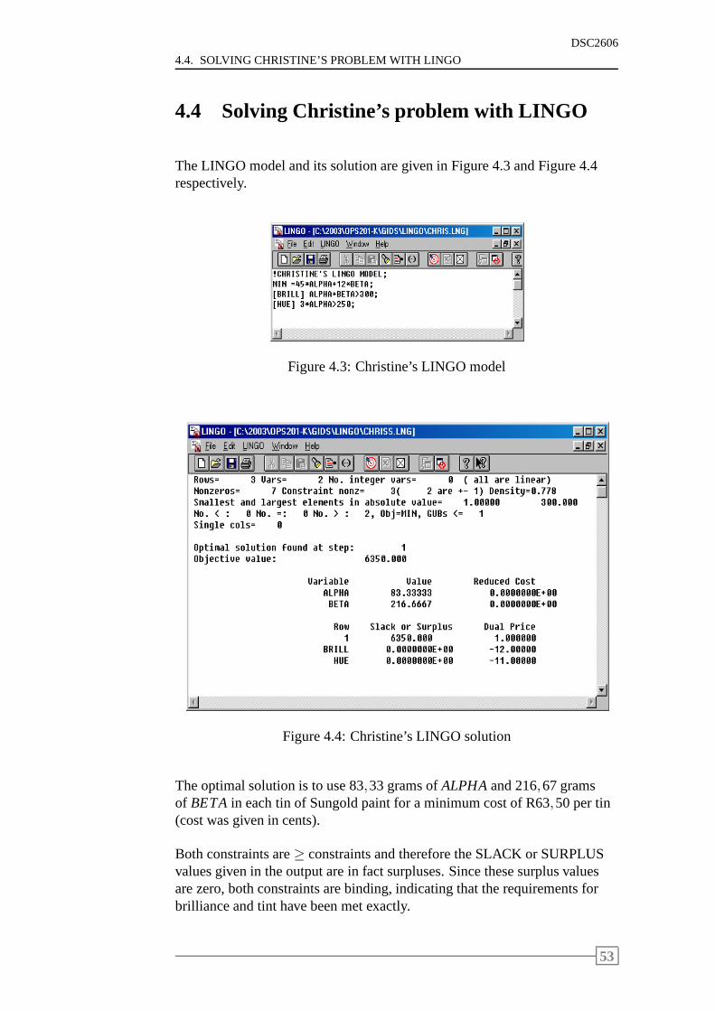
4.4. SOLVING CHRISTINE’S PROBLEM WITH LINGO
DSC2606
4.4 Solving Christine’s problem with LINGO
The LINGO model and its solution are given in Figure 4.3 and Figure 4.4respectively.
Figure 4.3: Christine’s LINGO model
Figure 4.4: Christine’s LINGO solution
The optimal solution is to use 83,33 grams ofALPHAand 216,67 gramsof BETAin each tin of Sungold paint for a minimum cost of R63,50 per tin(cost was given in cents).
Both constraints are≥ constraints and therefore the SLACK or SURPLUSvalues given in the output are in fact surpluses. Since thesesurplus valuesare zero, both constraints are binding, indicating that therequirements forbrilliance and tint have been met exactly.
53
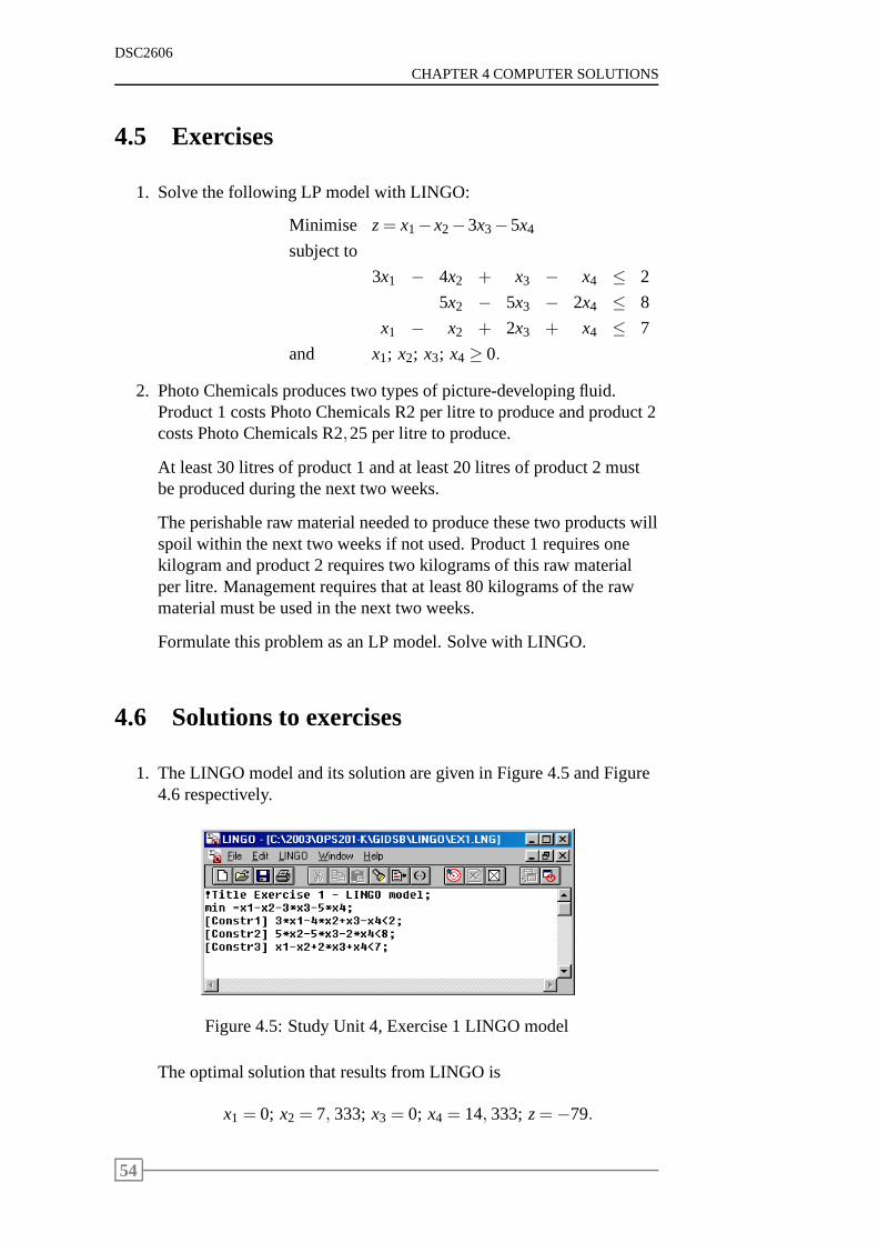
DSC2606
CHAPTER 4 COMPUTER SOLUTIONS
4.5 Exercises
1. Solve the following LP model with LINGO:
Minimise z= x1−x2−3x3−5x4
subject to
3x1 − 4x2 + x3 − x4 ≤ 2
5x2 − 5x3 − 2x4 ≤ 8
x1 − x2 + 2x3 + x4 ≤ 7
and x1; x2; x3; x4≥ 0.
2. Photo Chemicals produces two types of picture-developing fluid.Product 1 costs Photo Chemicals R2 per litre to produce and product 2costs Photo Chemicals R2,25 per litre to produce.
At least 30 litres of product 1 and at least 20 litres of product 2 mustbe produced during the next two weeks.
The perishable raw material needed to produce these two products willspoil within the next two weeks if not used. Product 1 requires onekilogram and product 2 requires two kilograms of this raw materialper litre. Management requires that at least 80 kilograms ofthe rawmaterial must be used in the next two weeks.
Formulate this problem as an LP model. Solve with LINGO.
4.6 Solutions to exercises
1. The LINGO model and its solution are given in Figure 4.5 andFigure4.6 respectively.
Figure 4.5: Study Unit 4, Exercise 1 LINGO model
The optimal solution that results from LINGO is
x1 = 0; x2 = 7, 333; x3 = 0; x4 = 14, 333; z=−79.
54
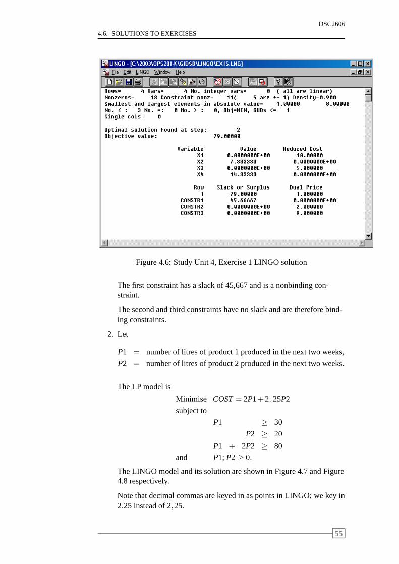
4.6. SOLUTIONS TO EXERCISES
DSC2606
Figure 4.6: Study Unit 4, Exercise 1 LINGO solution
The first constraint has a slack of 45,667 and is a nonbinding con-straint.
The second and third constraints have no slack and are therefore bind-ing constraints.
2. Let
P1 = number of litres of product 1 produced in the next two weeks,
P2 = number of litres of product 2 produced in the next two weeks.
The LP model is
Minimise COST= 2P1+2, 25P2
subject to
P1 ≥ 30
P2 ≥ 20
P1 + 2P2 ≥ 80
and P1; P2 ≥ 0.
The LINGO model and its solution are shown in Figure 4.7 and Figure4.8 respectively.
Note that decimal commas are keyed in as points in LINGO; we key in2.25 instead of 2,25.
55
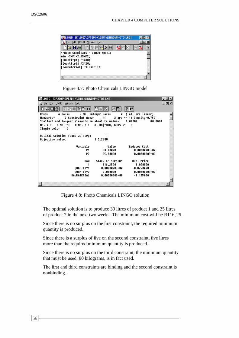
DSC2606
CHAPTER 4 COMPUTER SOLUTIONS
Figure 4.7: Photo Chemicals LINGO model
Figure 4.8: Photo Chemicals LINGO solution
The optimal solution is to produce 30 litres of product 1 and 25 litresof product 2 in the next two weeks. The minimum cost will be R116,25.
Since there is no surplus on the first constraint, the required minimumquantity is produced.
Since there is a surplus of five on the second constraint, five litresmore than the required minimum quantity is produced.
Since there is no surplus on the third constraint, the minimum quantitythat must be used, 80 kilograms, is in fact used.
The first and third constraints are binding and the second constraint isnonbinding.
56
Part 2
Nonlinear Programming
This part introduces the concept of nonlinear mathematicalprogram-ming..The concepts of a limit and the derivative of a function form back-ground knowledge. These concepts are discussed in Study unit 7 andin Study unit 8. You must familiarise yourself with this backgroundto limits and differentiation, but you will not be examined on thesetwo study units explicitly.You will however be examined explicitly on all of the material inall the other study units in this part.
57

58
Chapter 5
Introductory concepts
Contents5.1 Introduction . . . . . . . . . . . . . . . . . . . . . . . . 60
5.2 Linear versus nonlinear . . . . . . . . . . . . . . . . . . 61
5.3 Examples of NLP categories . . . . . . . . . . . . . . . 62
5.4 Assumptions of NLP . . . . . . . . . . . . . . . . . . . . 63
5.5 Solutions to models – basic concepts . . . . . . . . . . . 64
5.6 Exercises . . . . . . . . . . . . . . . . . . . . . . . . . . 64
5.7 Solutions to exercises . . . . . . . . . . . . . . . . . . . 65
59
DSC2606
CHAPTER 5 INTRODUCTORY CONCEPTS
Sections from prescribed book,WinstonChapter 11, Section 11.2
Learning objectives
After completing this study unit you should be able to
• understand the definitions of linear and nonlinear functions
• determine whether a function is linear or nonlinear
• distinguish between LP and NLP models
• identify the objective function and the constraints of an NLP model
• distinguish between constrained and unconstrained NLPs
• understand why NLPs do not necessarily satisfy the assumptions ofLPs
• check whether a particular point is in the feasible area of anNLP ornot (the same as for LP models)
• explain differences between LPs and NLPs concerning the positioningof the optimal solution on the feasible area
• explain what is meant by local extremum.
5.1 Introduction
In the first part of this study guide we studied linear programming (LP). Ourgoal was to optimise (maximise or minimise) the objective function sub-ject to constraints. The objective function and all the constraints werelinearequationsand/orlinear inequalities.
In many optimisation problems, however, the objective function may notbe a linear function and/or some or all of the constraints need not be linearequations and/or inequalities. Anoptimisation problem containing nonlin-ear equations and/or inequalities is called a nonlinear programming (NLP)problem.
In this second part of the study guide, we discuss techniquesthat are used tosolve NLP problems.
60
5.2. LINEAR VERSUS NONLINEAR
DSC2606
5.2 Linear versus nonlinear
In the LP part of this study guide we saw that a linear functionis one whereeach term is either a number or a number multiplied by a symbol. The termsdo not contain squares, exponents, cross-products, squareroots etc.
The definition of a linear function as given in the prescribedtextbook,Win-ston, is as follows:
Definition 5.1 A function f (x1; x2; . . . ; xn) of x1; x2; . . . ;xn is a linear func-tion if and only if for some set of constantsc1; c2; . . . ; cn,
f (x1; x2; . . . ; xn) = c1x1+c2x2+ · · ·+cnxn.
A function where some terms contain exponents, cross-products, squareroots etc is by implication a nonlinear function.
For example,f (x1; x2) = 3x1+2x2 is a linear function andf (x1; x2) = x1x32
is a nonlinear function ofx1 andx2.
Definition 5.2 For any linear functionf (x1; x2; . . . ; xn) and any numberb,the inequalities
f (x1; x2; . . . ; xn)≤ b
andf (x1; x2; . . . ; xn)≥ b,
are linear inequalities.
For example, 4x1+ 3x2 ≤ 3 and 2x1+ 5x2 ≥ 4 are linear inequalities, but
x121 x3
2≥ 5 is a nonlinear inequality.
The general form of an LP model was given in Section 2.5.
Winstongives the general form of an NLP as follows:
61
DSC2606
CHAPTER 5 INTRODUCTORY CONCEPTS
Definition 5.3 A generalnonlinear programming problem (NLP) (la-belled(1)) can be expressed as follows:
Find the values of decision variablesx1; x2; . . . ; xn that
max (or min) z= f (x1; x2; . . . ; xn)
subject to g1(x1; x2; . . . ; xn) (≤,=, or ≥) b1
g2(x1; x2; . . . ; xn) (≤,=, or ≥) b2
...
gm(x1; x2; . . . ; xn) (≤,=, or ≥) bm.
As in LP, the function
z= f (x1; x2; . . . ; xn)
is the NLP’sobjective function, and
g1(x1; x2; . . . ; xn) (≤,=, or ≥) b1
......
...
gm(x1; x2; . . . ; xn) (≤,=, or ≥) bm
are the NLP’sconstraints. Such an NLP is called aconstrained NLP.
If an NLP does not have any constraints, it is called anunconstrained NLP.
Obviously if f ; g1; g2; . . . ; gm are all linear functions, then(1) is a linearprogramming model.
5.3 Examples of NLP categories
Nonlinear programming models fall into one of two categories; constrainedNLPs or unconstrained NLPs.
Winstongives the following example of an unconstrained NLP:
Example 5.1
It costs a companyc rand to produce one unit of a product. The de-mand for the product depends on the price charged per unit,p rand,and this relationship isD(p).
The company wants to know what price per unit to charge for theproduct so as to maximise its profit.
62
5.4. ASSUMPTIONS OF NLP
DSC2606
Solution
The company’s decision variable isp. The profit function is
P(p) = Profit per unit× number demanded
= (p−c)×D(p).
Therefore, the company must maximise the following unconstrained NLP:
MaximiseP(p) = (p−c)D(p).
Winstongives the following example of a constrained NLP:
Example 5.2
A company can produceKL units of a product ifK units of capital andL units of labour are used. Capital can be purchased at R4 per unit andlabour at R1 per unit. A total of R8 is available to purchase capital andlabour.
The company wants to maximise the quantity of products manufac-tured.
Solution
Let K andL represent the quantities of capital and labour purchased, respec-tively. ThenK andL must satisfy 4K+L≤ 8, K ≥ 0 andL≥ 0.
Therefore, the company must maximise the following constrained NLP:
Maximise Z = KL
subject to
4K + L ≤ 8
and K; L≥ 0.
5.4 Assumptions of NLP
In the first part of this study guide we saw that for an LP model to be an ap-propriate representation of a real-life situation, certain assumptions must besatisfied.
Unlike an LP, an NLP may not satisfy the Proportionality and Additivityassumptions.
If we refer back to Example 5.2, we see that if we increaseL by one unit,thenZ increases byK units. Therefore, the effect on the objective function
63
DSC2606
CHAPTER 5 INTRODUCTORY CONCEPTS
value,Z, of increasingL by one depends onK. This means that the Additiv-ity assumption is not satisfied.
Consider the following NLP:
Maximise z= x13 +y
13
subject to
x + y = 1
and x; y≥ 0.
Doubling the value ofx does not double the contribution ofx to the objectivefunction value,z. Therefore, the Proportionality assumption is not satisfied.
5.5 Solutions to models – basic concepts
Refer toWinston, Section 11.2 and study the following:
• a feasible region
• an optimal solution
• differences between LPs and NLPs concerning the positioning of theoptimal solution on the feasible region
• local extremum.
You will find the exact page references in Tutorial Letter 101.
5.6 Exercises
1. For each of the following functions, state whether the function is lin-ear or nonlinear:
(a) f (x) = ex
(b) g(y) = y2+2y+4
(c) f (K;L) = 4K +L
(d) F(K;L) = KL
(e) g(x;y) = x13 +y
13
(f) h(x;y) = x+y
(g) Z(A;A1;A2) =0,04A1+0,01A2
A
(h) Z(A1;A2) =0,04A1+0,01A2
0,01
(i) D(X;Y) = (X−5)2+(Y−5)2
64
5.7. SOLUTIONS TO EXERCISES
DSC2606
(j) d(X;Y) =√
(X−5)+(Y−5)
2. Consider the following NLP model:
Minimise Z = (x−1)2+(y−1)2
subject to
x − 2y ≥ −2
x + 2y ≤ 10
x − y ≤ 4
x ≥ 2
y ≥ 0.
(a) Are the following points in the feasible area or not?
(6;1), (6;2), (3;1), (3;3), (2;1);(2;2)
(b) For each of the feasible points in (a), calculate the objective func-tion value.
(c) With the information available from (a) and (b), can we say thatthe point(2;1) is a local minimum of the NLP?
5.7 Solutions to exercises
1. (a) Nonlinear
(b) Nonlinear
(c) Linear
(d) Nonlinear
(e) Nonlinear
(f) Linear
(g) Nonlinear
(h) Linear
(i) Nonlinear
(j) Nonlinear
2. (a) For a point to be in the feasible area, it must satisfy all five of theconstraints.
Consider point(6;1).
Constraint 1:x−2y= 6−2(1) = 4>−2 ⇒ satisfied
65
DSC2606
CHAPTER 5 INTRODUCTORY CONCEPTS
Constraint 2:x+2y= 6+2(1) = 8< 10 ⇒ satisfied
Constraint 3:x−y= 6−1= 5� 4 ⇒ not satisfied
The third constraint is not satisfied. Therefore, point(6;1) is notin the feasible area.
Consider point(6;2).
Constraint 1: 6−2(2) = 2>−2 ⇒ satisfied
Constraint 2: 6+2(2) = 10= 10 ⇒ satisfied
Constraint 3: 6−2= 4= 4 ⇒ satisfied
Constraint 4: 6> 2 ⇒ satisfied
Constraint 5: 2> 0 ⇒ satisfied
All five constraints are satisfied. Therefore, point(6;2) is in thefeasible area.
If we apply this method to the remaining points, we obtain thefollowing result:
The points in the feasible area are(6;2), (3;1), (2;2) and(2;1).
The points not in the feasible area are(6;1) and(3;3).
(b) The objective function values of the feasible points areas fol-lows:
Point(6;2):
Z = (x−1)2+(y−1)2
= (6−1)2+(2−1)2
= 52+12
= 26
Point(3;1):Z = (3−1)2+(1−1)2 = 4
Point(2;2):Z = (2−1)2+(2−1)2 = 2
Point(2;1):Z = (2−1)2+(1−1)2 = 1
(c) No, even though the objective function value at the point(2;1)is less than any other point considered, we have not looked atallfeasible points in the neighbourhood of(2;1).
66
Chapter 6
Formulating NLP models andcomputer solutions
Contents6.1 Introduction . . . . . . . . . . . . . . . . . . . . . . . . 68
6.2 A dimensions problem . . . . . . . . . . . . . . . . . . . 68
6.3 An inventory problem . . . . . . . . . . . . . . . . . . . 70
6.4 LINGO . . . . . . . . . . . . . . . . . . . . . . . . . . . 71
6.5 Formulation and LINGO solution of NLP models . . . 74
6.6 Exercises . . . . . . . . . . . . . . . . . . . . . . . . . . 75
6.7 Solutions to exercises . . . . . . . . . . . . . . . . . . . 75
6.8 Looking ahead at the remaining study units . . . . . . . 77
67
DSC2606
CHAPTER 6 FORMULATING NLP MODELS AND COMPUTER SOLUTIONS
Sections from prescribed book,WinstonChapter 11, Section 11.2
Learning objectivesAfter completing this study unit you should be able to
• formulate an NLP model for a given problem
• solve an NLP model with LINGO.
6.1 Introduction
In Part 1 of this study guide, the formulation (modelling) process, that is, theconstruction of models to represent problem situations, was described in de-tail and many examples were given. Only linear functions were consideredin this section. The principles and guidelines given there for modelling are,however, also applicable when modelling nonlinear functions.
You should refer back to the relevant study units to refresh your memory.
We will now illustrate the modelling of problem situations where nonlinearfunctions are involved by means of two problems: a dimensions problemand an inventory problem.
6.2 A dimensions problem
A rectangular piece of cardboard, which is 16 centimetres long and 10 cen-timetres wide, must be turned into an open box. This can be done by cuttingaway identical squares from each corner of the cardboard andfolding up theresultant flaps.
We want to find the dimensions of the box that will yield the maximum vol-ume for the box.
Decision variable
Let x denote the length (in centimetres) of one side of each of the identicalsquares to be cut out of the cardboard.
This problem is illustrated in Figure 6.1.
68
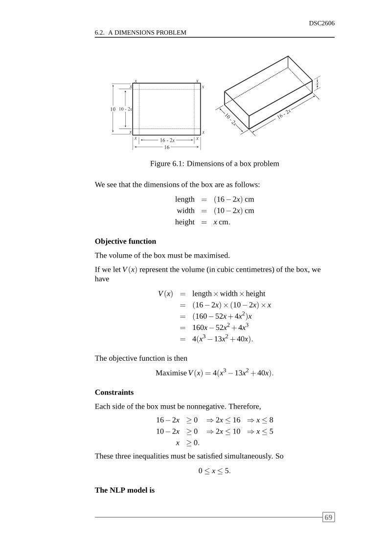
6.2. A DIMENSIONS PROBLEM
DSC2606
1 6 - 2 x
x
x x
x
x
xx
x
1 6
1 0 1 0 - 2 x
x
Figure 6.1: Dimensions of a box problem
We see that the dimensions of the box are as follows:
length = (16−2x) cm
width = (10−2x) cm
height = x cm.
Objective function
The volume of the box must be maximised.
If we letV(x) represent the volume (in cubic centimetres) of the box, wehave
V(x) = length×width×height
= (16−2x)× (10−2x)×x
= (160−52x+4x2)x
= 160x−52x2+4x3
= 4(x3−13x2+40x).
The objective function is then
MaximiseV(x) = 4(x3−13x2+40x).
Constraints
Each side of the box must be nonnegative. Therefore,
16−2x ≥ 0 ⇒ 2x≤ 16 ⇒ x≤ 8
10−2x ≥ 0 ⇒ 2x≤ 10 ⇒ x≤ 5
x ≥ 0.
These three inequalities must be satisfied simultaneously.So
0≤ x≤ 5.
The NLP model is
69
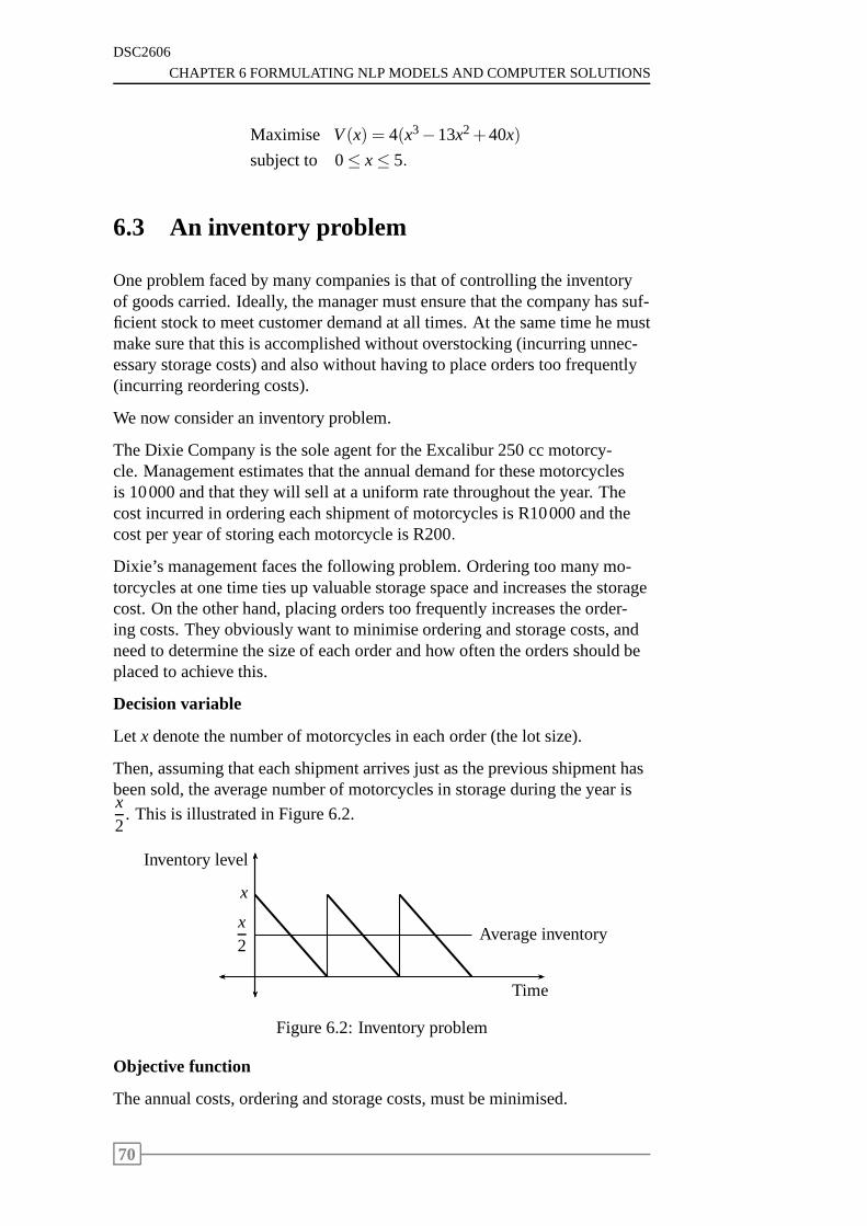
DSC2606
CHAPTER 6 FORMULATING NLP MODELS AND COMPUTER SOLUTIONS
Maximise V(x) = 4(x3−13x2+40x)
subject to 0≤ x≤ 5.
6.3 An inventory problem
One problem faced by many companies is that of controlling the inventoryof goods carried. Ideally, the manager must ensure that the company has suf-ficient stock to meet customer demand at all times. At the sametime he mustmake sure that this is accomplished without overstocking (incurring unnec-essary storage costs) and also without having to place orders too frequently(incurring reordering costs).
We now consider an inventory problem.
The Dixie Company is the sole agent for the Excalibur 250 cc motorcy-cle. Management estimates that the annual demand for these motorcyclesis 10000 and that they will sell at a uniform rate throughout the year. Thecost incurred in ordering each shipment of motorcycles is R10000 and thecost per year of storing each motorcycle is R200.
Dixie’s management faces the following problem. Ordering too many mo-torcycles at one time ties up valuable storage space and increases the storagecost. On the other hand, placing orders too frequently increases the order-ing costs. They obviously want to minimise ordering and storage costs, andneed to determine the size of each order and how often the orders should beplaced to achieve this.
Decision variable
Let x denote the number of motorcycles in each order (the lot size).
Then, assuming that each shipment arrives just as the previous shipment hasbeen sold, the average number of motorcycles in storage during the year isx2
. This is illustrated in Figure 6.2.
Time
Inventory level
Average inventoryx2
x
Figure 6.2: Inventory problem
Objective function
The annual costs, ordering and storage costs, must be minimised.
70
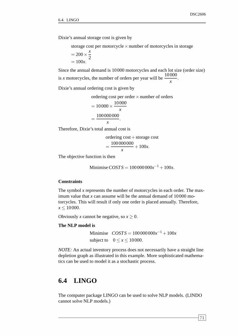
6.4. LINGO
DSC2606
Dixie’s annual storage cost is given by
storage cost per motorcycle×number of motorcycles in storage
= 200× x2
= 100x.
Since the annual demand is 10000 motorcycles and each lot size (order size)
is x motorcycles, the number of orders per year will be10000
x.
Dixie’s annual ordering cost is given by
ordering cost per order×number of orders
= 10000× 10000x
=100000000
x.
Therefore, Dixie’s total annual cost is
ordering cost+storage cost
=100000000
x+100x.
The objective function is then
MinimiseCOSTS= 100000000x−1+100x.
Constraints
The symbolx represents the number of motorcycles in each order. The max-imum value thatx can assume will be the annual demand of 10000 mo-torcycles. This will result if only one order is placed annually. Therefore,x≤ 10000.
Obviouslyx cannot be negative, sox≥ 0.
The NLP model is
Minimise COSTS= 100000000x−1+100x
subject to 0≤ x≤ 10000.
NOTE:An actual inventory process does not necessarily have a straight linedepletion graph as illustrated in this example. More sophisticated mathema-tics can be used to model it as a stochastic process.
6.4 LINGO
The computer package LINGO can be used to solve NLP models. (LINDOcannot solve NLP models.)
71
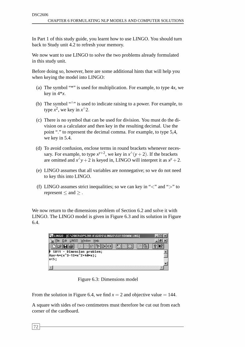
DSC2606
CHAPTER 6 FORMULATING NLP MODELS AND COMPUTER SOLUTIONS
In Part 1 of this study guide, you learnt how to use LINGO. You should turnback to Study unit 4.2 to refresh your memory.
We now want to use LINGO to solve the two problems already formulatedin this study unit.
Before doing so, however, here are some additional hints that will help youwhen keying the model into LINGO:
(a) The symbol “*” is used for multiplication. For example, to type 4x, wekey in 4*x.
(b) The symbol “∧” is used to indicate raising to a power. For example, totypex2, we key inx∧2.
(c) There is no symbol that can be used for division. You must do the di-vision on a calculator and then key in the resulting decimal.Use thepoint “.” to represent the decimal comma. For example, to type 5,4,we key in 5.4.
(d) To avoid confusion, enclose terms in round brackets whenever neces-sary. For example, to typexy+2, we key inx∧(y+ 2). If the bracketsare omitted andx∧y+2 is keyed in, LINGO will interpret it asxy+2.
(e) LINGO assumes that all variables are nonnegative; so we do not needto key this into LINGO.
(f) LINGO assumes strict inequalities; so we can key in “<” and “>” torepresent≤ and≥ .
We now return to the dimensions problem of Section 6.2 and solve it withLINGO. The LINGO model is given in Figure 6.3 and its solutionin Figure6.4.
Figure 6.3: Dimensions model
From the solution in Figure 6.4, we findx= 2 and objective value= 144.
A square with sides of two centimetres must therefore be cut out from eachcorner of the cardboard.
72
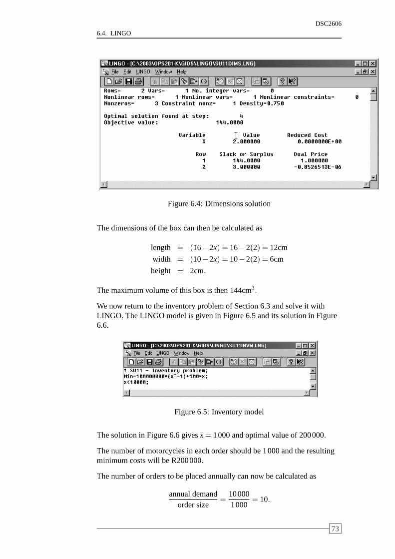
6.4. LINGO
DSC2606
Figure 6.4: Dimensions solution
The dimensions of the box can then be calculated as
length = (16−2x) = 16−2(2) = 12cm
width = (10−2x) = 10−2(2) = 6cm
height = 2cm.
The maximum volume of this box is then 144cm3.
We now return to the inventory problem of Section 6.3 and solve it withLINGO. The LINGO model is given in Figure 6.5 and its solutionin Figure6.6.
Figure 6.5: Inventory model
The solution in Figure 6.6 givesx= 1000 and optimal value of 200000.
The number of motorcycles in each order should be 1000 and theresultingminimum costs will be R200000.
The number of orders to be placed annually can now be calculated as
annual demandorder size
=100001000
= 10.
73
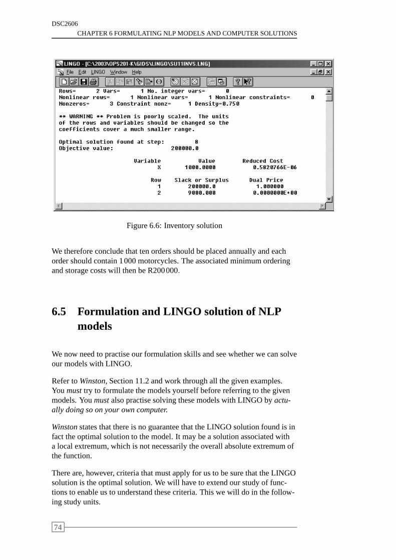
DSC2606
CHAPTER 6 FORMULATING NLP MODELS AND COMPUTER SOLUTIONS
Figure 6.6: Inventory solution
We therefore conclude that ten orders should be placed annually and eachorder should contain 1000 motorcycles. The associated minimum orderingand storage costs will then be R200000.
6.5 Formulation and LINGO solution of NLPmodels
We now need to practise our formulation skills and see whether we can solveour models with LINGO.
Refer toWinston, Section 11.2 and work through all the given examples.You musttry to formulate the models yourself before referring to thegivenmodels. Youmustalso practise solving these models with LINGO byactu-ally doing so on your own computer.
Winstonstates that there is no guarantee that the LINGO solution found is infact the optimal solution to the model. It may be a solution associated witha local extremum, which is not necessarily the overall absolute extremum ofthe function.
There are, however, criteria that must apply for us to be surethat the LINGOsolution is the optimal solution. We will have to extend our study of func-tions to enable us to understand these criteria. This we willdo in the follow-ing study units.
74
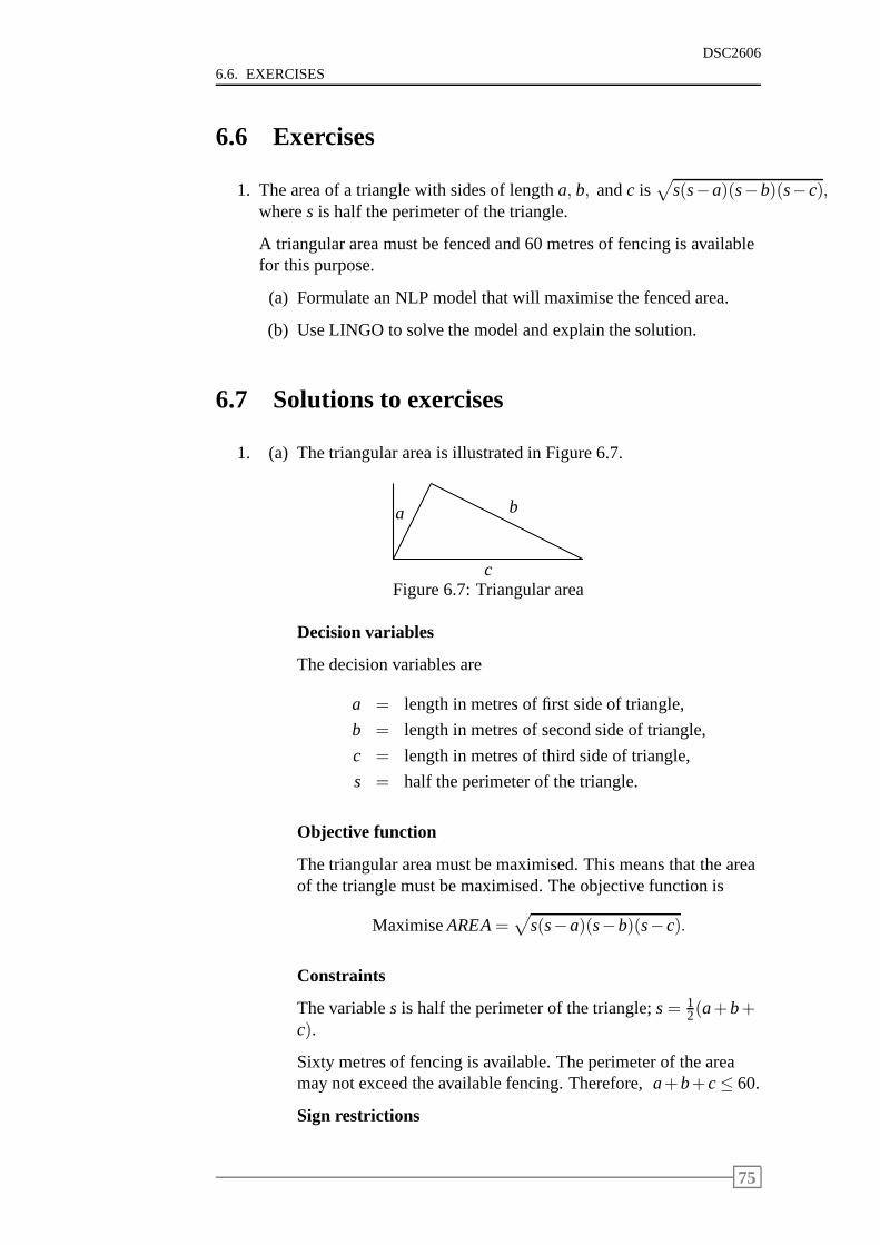
6.6. EXERCISES
DSC2606
6.6 Exercises
1. The area of a triangle with sides of lengtha, b, andc is√
s(s−a)(s−b)(s−c),wheres is half the perimeter of the triangle.
A triangular area must be fenced and 60 metres of fencing is availablefor this purpose.
(a) Formulate an NLP model that will maximise the fenced area.
(b) Use LINGO to solve the model and explain the solution.
6.7 Solutions to exercises
1. (a) The triangular area is illustrated in Figure 6.7.
a b
cFigure 6.7: Triangular area
Decision variables
The decision variables are
a = length in metres of first side of triangle,
b = length in metres of second side of triangle,
c = length in metres of third side of triangle,
s = half the perimeter of the triangle.
Objective function
The triangular area must be maximised. This means that the areaof the triangle must be maximised. The objective function is
MaximiseAREA=√
s(s−a)(s−b)(s−c).
Constraints
The variables is half the perimeter of the triangle;s= 12(a+b+
c).
Sixty metres of fencing is available. The perimeter of the areamay not exceed the available fencing. Therefore,a+b+c≤ 60.
Sign restrictions
75
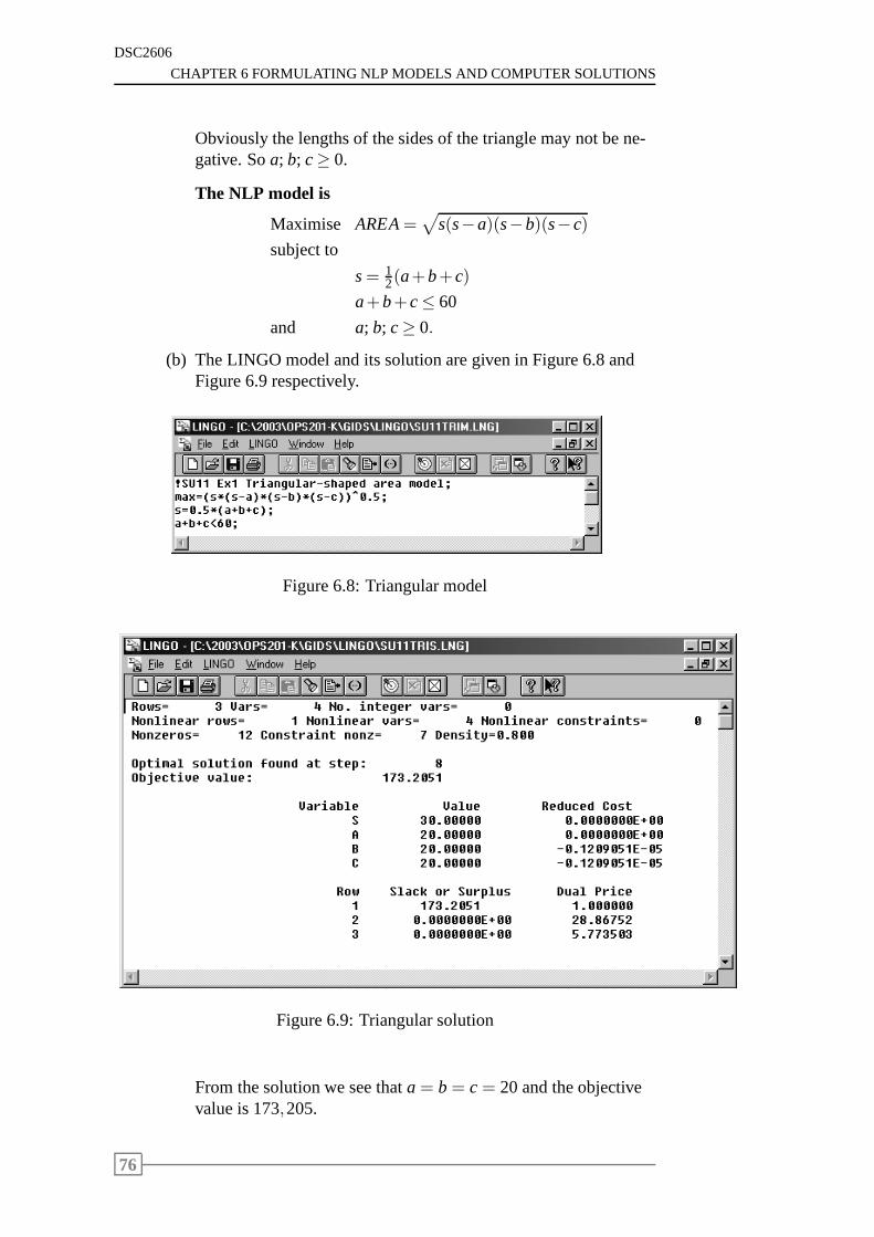
DSC2606
CHAPTER 6 FORMULATING NLP MODELS AND COMPUTER SOLUTIONS
Obviously the lengths of the sides of the triangle may not be ne-gative. Soa; b; c≥ 0.
The NLP model is
Maximise AREA=√
s(s−a)(s−b)(s−c)
subject to
s= 12(a+b+c)
a+b+c≤ 60
and a; b; c≥ 0.
(b) The LINGO model and its solution are given in Figure 6.8 andFigure 6.9 respectively.
Figure 6.8: Triangular model
Figure 6.9: Triangular solution
From the solution we see thata = b = c = 20 and the objectivevalue is 173,205.
76
6.8. LOOKING AHEAD AT THE REMAINING STUDY UNITS
DSC2606
This means that a maximum area of 173,205 square metres willbe fenced if the sides of the triangle are all of equal length,thatis, 20 metres.
6.8 Looking ahead at the remaining study units
The objective functions we encountered when formulating NLP models wereeitherfunctions of one variable only(eg the dimensions of the box problemand the inventory problem), orfunctions of several variables(eg Oilco’sproblem inWinstonand the triangular area problem).
We also saw that we can conclude that the solution obtained with LINGO isindeed the optimal solution to the model only if certain criteria apply, andthat we will have to extend our study of functions, of one and several vari-ables, to understand these criteria.
In the following study units we will return to the basics of functions and howto solve them. To do this we need differential calculus.
We start off by introducing differential calculus by considering functions ofone variable only. After covering the basic concepts (Studyunits 7–10), wewill proceed to the practical applications (Study units 11–14). We will alsointroduce integral calculus and its practical applications (Study unit 15).
In later study units we proceed to functions of several variables; first cov-ering the basic concepts of partial differential calculus (Study unit 16) andthen the practical applications (Study units 17–20).
77

DSC2606
CHAPTER 6 FORMULATING NLP MODELS AND COMPUTER SOLUTIONS
78
Chapter 7
Limits and continuity
Contents7.1 Introduction . . . . . . . . . . . . . . . . . . . . . . . . 80
7.2 The limit of a function . . . . . . . . . . . . . . . . . . . 80
7.3 Infinite limits . . . . . . . . . . . . . . . . . . . . . . . . 90
7.4 Limits when x tends to infinity . . . . . . . . . . . . . . 92
7.5 Continuity . . . . . . . . . . . . . . . . . . . . . . . . . 94
7.6 Exercises . . . . . . . . . . . . . . . . . . . . . . . . . . 97
7.7 Solutions to exercises . . . . . . . . . . . . . . . . . . . 101
79
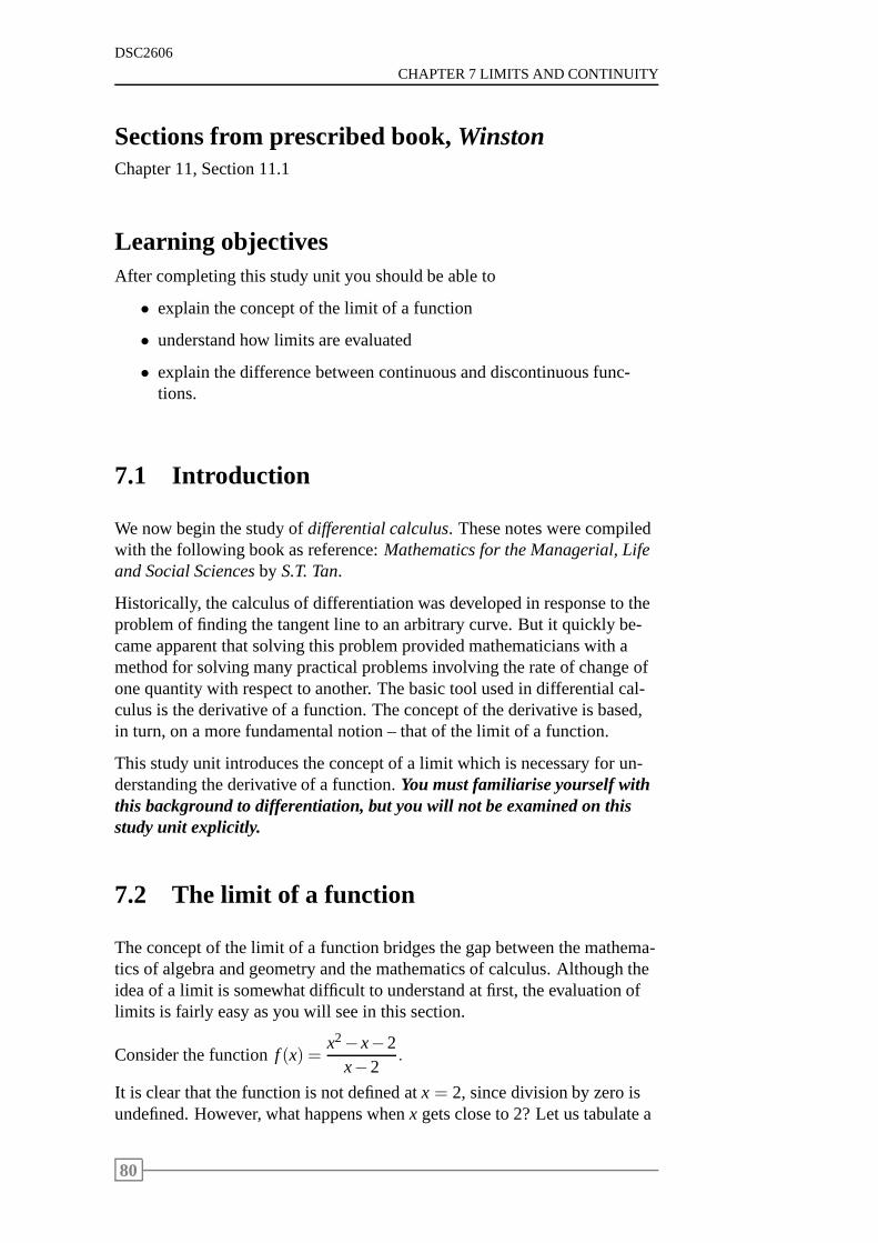
DSC2606
CHAPTER 7 LIMITS AND CONTINUITY
Sections from prescribed book,WinstonChapter 11, Section 11.1
Learning objectivesAfter completing this study unit you should be able to
• explain the concept of the limit of a function
• understand how limits are evaluated
• explain the difference between continuous and discontinuous func-tions.
7.1 Introduction
We now begin the study ofdifferential calculus. These notes were compiledwith the following book as reference:Mathematics for the Managerial, Lifeand Social Sciencesby S.T. Tan.
Historically, the calculus of differentiation was developed in response to theproblem of finding the tangent line to an arbitrary curve. Butit quickly be-came apparent that solving this problem provided mathematicians with amethod for solving many practical problems involving the rate of change ofone quantity with respect to another. The basic tool used in differential cal-culus is the derivative of a function. The concept of the derivative is based,in turn, on a more fundamental notion – that of the limit of a function.
This study unit introduces the concept of a limit which is necessary for un-derstanding the derivative of a function.You must familiarise yourself withthis background to differentiation, but you will not be examined on thisstudy unit explicitly.
7.2 The limit of a function
The concept of the limit of a function bridges the gap betweenthe mathema-tics of algebra and geometry and the mathematics of calculus. Although theidea of a limit is somewhat difficult to understand at first, the evaluation oflimits is fairly easy as you will see in this section.
Consider the functionf (x) =x2−x−2
x−2.
It is clear that the function is not defined atx = 2, since division by zero isundefined. However, what happens whenx gets close to 2? Let us tabulate a
80
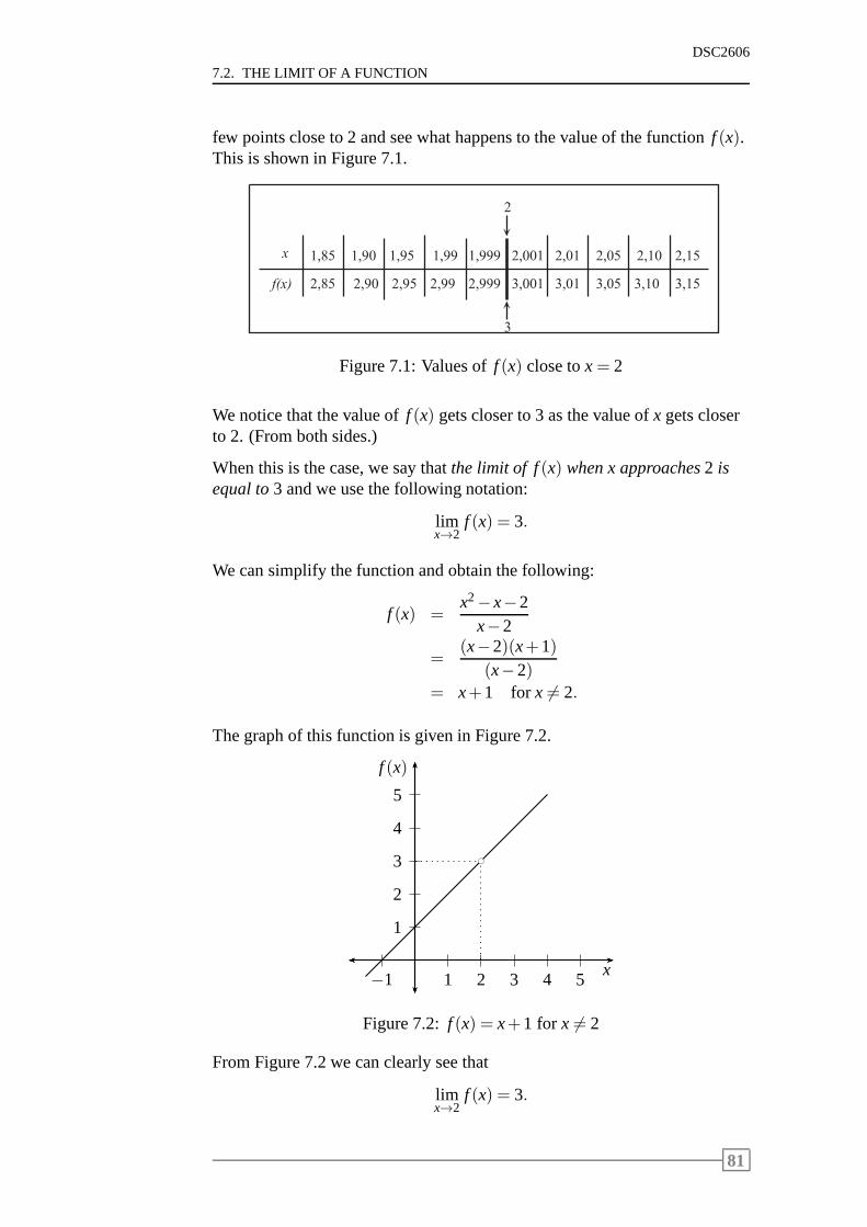
7.2. THE LIMIT OF A FUNCTION
DSC2606
few points close to 2 and see what happens to the value of the function f (x).This is shown in Figure 7.1.
x
f ( x )
1 , 8 5
2 , 8 5
1 , 9 0
2 , 9 0
1 , 9 5
2 , 9 5
1 , 9 9
2 , 9 9
1 , 9 9 9
2 , 9 9 9
2 , 0 0 1
3 , 0 0 1
2 , 0 1
3 , 0 1
2 , 0 5
3 , 0 5
2 , 1 0
3 , 1 0
2 , 1 5
3 , 1 5
2
3
Figure 7.1: Values off (x) close tox= 2
We notice that the value off (x) gets closer to 3 as the value ofx gets closerto 2. (From both sides.)
When this is the case, we say thatthe limit of f(x) when x approaches2 isequal to3 and we use the following notation:
limx→2
f (x) = 3.
We can simplify the function and obtain the following:
f (x) =x2−x−2
x−2
=(x−2)(x+1)
(x−2)= x+1 for x 6= 2.
The graph of this function is given in Figure 7.2.
1
2
3
4
5
1 2 3 4 5−1x
f (x)
bc
Figure 7.2: f (x) = x+1 for x 6= 2
From Figure 7.2 we can clearly see that
limx→2
f (x) = 3.
81
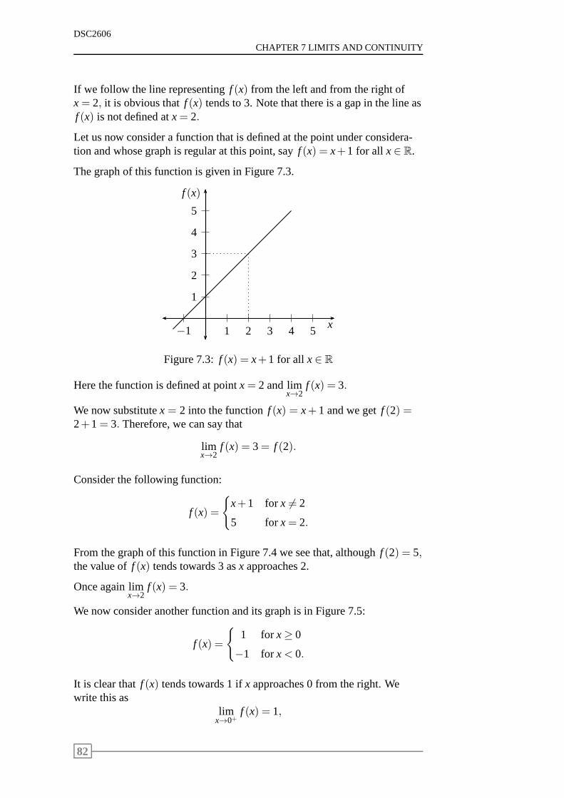
DSC2606
CHAPTER 7 LIMITS AND CONTINUITY
If we follow the line representingf (x) from the left and from the right ofx= 2, it is obvious thatf (x) tends to 3. Note that there is a gap in the line asf (x) is not defined atx= 2.
Let us now consider a function that is defined at the point under considera-tion and whose graph is regular at this point, sayf (x) = x+1 for all x∈ R.
The graph of this function is given in Figure 7.3.
1
2
3
4
5
1 2 3 4 5−1x
f (x)
Figure 7.3: f (x) = x+1 for all x∈ R
Here the function is defined at pointx= 2 and limx→2
f (x) = 3.
We now substitutex = 2 into the functionf (x) = x+1 and we getf (2) =2+1= 3. Therefore, we can say that
limx→2
f (x) = 3= f (2).
Consider the following function:
f (x) =
{
x+1 for x 6= 2
5 for x= 2.
From the graph of this function in Figure 7.4 we see that, although f (2) = 5,the value off (x) tends towards 3 asx approaches 2.
Once again limx→2
f (x) = 3.
We now consider another function and its graph is in Figure 7.5:
f (x) =
{
1 for x≥ 0
−1 for x< 0.
It is clear thatf (x) tends towards 1 ifx approaches 0 from the right. Wewrite this as
limx→0+
f (x) = 1,
82
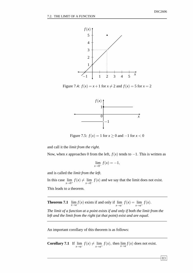
7.2. THE LIMIT OF A FUNCTION
DSC2606
1
2
3
4
5
1 2 3 4 5−1x
f (x)
bc
b
Figure 7.4: f (x) = x+1 for x 6= 2 and f (x) = 5 for x= 2
x
f (x)
1
0
−1
b
bc
Figure 7.5: f (x) = 1 for x≥ 0 and−1 for x< 0
and call it thelimit from the right.
Now, whenx approaches 0 from the left,f (x) tends to−1. This is written as
limx→0−
f (x) =−1,
and is called thelimit from the left.
In this case limx→0+
f (x) 6= limx→0−
f (x) and we say that the limit does not exist.
This leads to a theorem.
Theorem 7.1 limx→a
f (x) exists if and only if limx→a−
f (x) = limx→a+
f (x).
The limit of a function at a point exists if and only if both thelimit from theleft and the limit from the right (at that point) exist and areequal.
An important corollary of this theorem is as follows:
Corollary 7.1 If limx→a−
f (x) 6= limx→a+
f (x), then limx→a
f (x) does not exist.
83
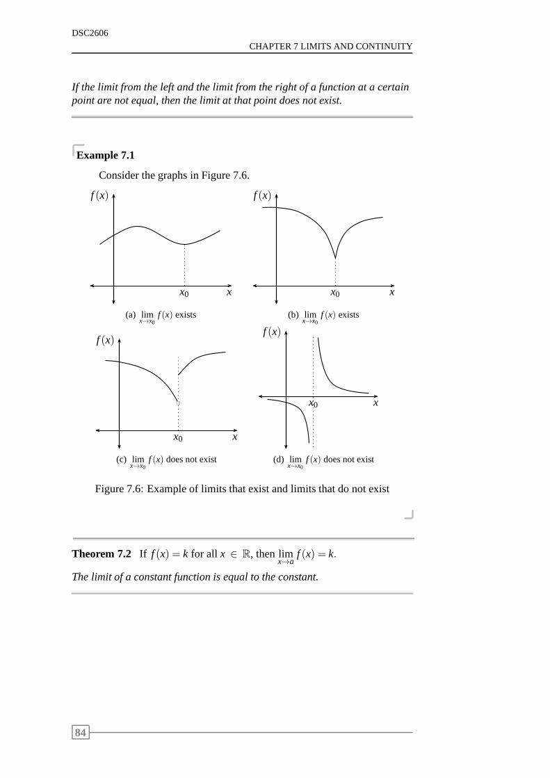
DSC2606
CHAPTER 7 LIMITS AND CONTINUITY
If the limit from the left and the limit from the right of a function at a certainpoint are not equal, then the limit at that point does not exist.
Example 7.1
Consider the graphs in Figure 7.6.
x
f (x)
x0
(a) limx→x0
f (x) exists
x
f (x)
x0
(b) limx→x0
f (x) exists
x
f (x)
x0
bc
(c) limx→x0
f (x) does not exist
x
f (x)
x0
(d) limx→x0
f (x) does not exist
Figure 7.6: Example of limits that exist and limits that do not exist
Theorem 7.2 If f (x) = k for all x ∈ R, then limx→a
f (x) = k.
The limit of a constant function is equal to the constant.
84
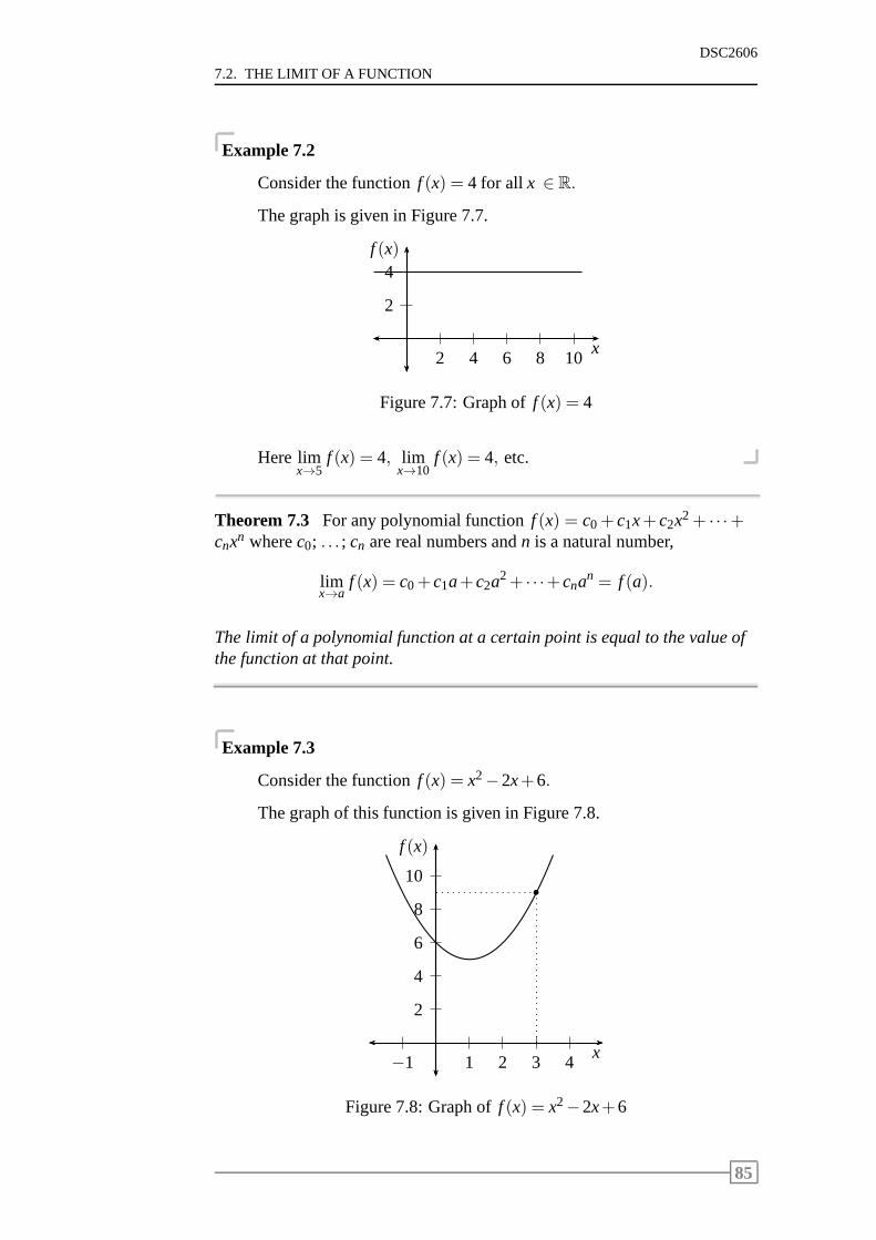
7.2. THE LIMIT OF A FUNCTION
DSC2606
Example 7.2
Consider the functionf (x) = 4 for all x ∈ R.
The graph is given in Figure 7.7.
2
4
2 4 6 8 10x
f (x)
Figure 7.7: Graph off (x) = 4
Here limx→5
f (x) = 4, limx→10
f (x) = 4, etc.
Theorem 7.3 For any polynomial functionf (x) = c0+ c1x+ c2x2+ · · ·+cnxn wherec0; . . . ; cn are real numbers andn is a natural number,
limx→a
f (x) = c0+c1a+c2a2+ · · ·+cnan = f (a).
The limit of a polynomial function at a certain point is equalto the value ofthe function at that point.
Example 7.3
Consider the functionf (x) = x2−2x+6.
The graph of this function is given in Figure 7.8.
2
4
6
8
10
1 2 3 4−1x
f (x)
b
Figure 7.8: Graph off (x) = x2−2x+6
85
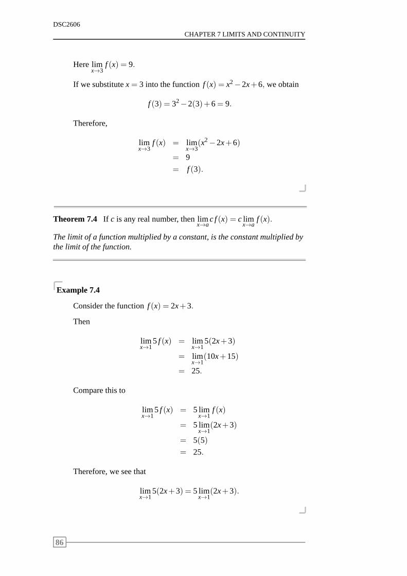
DSC2606
CHAPTER 7 LIMITS AND CONTINUITY
Here limx→3
f (x) = 9.
If we substitutex= 3 into the functionf (x) = x2−2x+6, we obtain
f (3) = 32−2(3)+6= 9.
Therefore,
limx→3
f (x) = limx→3
(x2−2x+6)
= 9
= f (3).
Theorem 7.4 If c is any real number, then limx→a
c f(x) = c limx→a
f (x).
The limit of a function multiplied by a constant, is the constant multiplied bythe limit of the function.
Example 7.4
Consider the functionf (x) = 2x+3.
Then
limx→1
5 f (x) = limx→1
5(2x+3)
= limx→1
(10x+15)
= 25.
Compare this to
limx→1
5 f (x) = 5 limx→1
f (x)
= 5 limx→1
(2x+3)
= 5(5)
= 25.
Therefore, we see that
limx→1
5(2x+3) = 5 limx→1
(2x+3).
86
7.2. THE LIMIT OF A FUNCTION
DSC2606
Theorem 7.5 If limx→a
f (x) and limx→a
g(x) exists, then
limx→a
[ f (x)+g(x)] = limx→a
f (x)+ limx→a
g(x).
The limit of the sum of two (or more) functions is equal to the sum of theirlimits.
Example 7.5
Consider the functionsf (x) = 2x+3 and g(x) = x+1.
Then
limx→1
[5 f (x)+g(x)] = limx→1
[5(2x+3)+(x+1)]
= limx→1
(10x+15+x+1)
= limx→1
(11x+16)
= 27.
Compare this to
limx→1
[5 f (x)+g(x)] = limx→1
5 f (x)+ limx→1
g(x)
= 5 limx→1
f (x)+ limx→1
g(x)
= 5 limx→1
(2x+3)+ limx→1
(x+1)
= 5(5)+2
= 27.
Therefore, we see that
limx→1
[5(2x+3)+(x+1)] = 5 limx→1
(2x+3)+ limx→1
(x+1).
Theorem 7.6 If limx→a
f (x) and limx→a
g(x) exist, then
limx→a
[ f (x)×g(x)] = [limx→a
f (x)]× [limx→a
g(x)].
The limit of the product of two (or more) functions is equal tothe product ofthe limits of the functions.
87
DSC2606
CHAPTER 7 LIMITS AND CONTINUITY
Example 7.6
Consider the functionsf (x) = 2x+3 and g(x) =x2−1x−1
.
Then
limx→1
5 f (x)g(x) = limx→1
5(2x+3)(x2−1)x−1
= limx→1
5(2x+3)(x−1)(x+1)(x−1)
= limx→1
5(2x+3)(x+1)
= 5(5)(2)
= 50.
Compare this to
limx→1
5 f (x)g(x) = limx→1
5 f (x)× limx→1
g(x)
= 5 limx→1
f (x)× limx→1
g(x)
= 5 limx→1
(2x+3)× limx→1
(
x2−1x−1
)
= 5 limx→1
(2x+3)× limx→1
(x−1)(x+1)(x−1)
= 5 limx→1
(2x+3)× limx→1
(x+1)
= 5(5)×2
= 50.
Therefore, we see that
limx→1
5(2x+3)(x2−1)(x−1)
= 5 limx→1
(2x+3)× limx→1
(x2−1)(x−1)
.
Theorem 7.7 If limx→a
f (x) exists, then
limx→a
[ f (x)]n =[
limx→a
f (x)]n
.
The limit of a function to the power n is equal to the limit of the function, tothe power n.
88
7.2. THE LIMIT OF A FUNCTION
DSC2606
Example 7.7
Consider the functionf (x) = x2+1.
Then
limx→2
[ f (x)]4 = limx→2
(x2+1)4
= (22+1)4
= 625.
Compare this to
limx→2
[ f (x)]4 =
[
limx→2
f (x)
]4
=
[
limx→2
(x2+1)
]4
= (22+1)4
= 625.
Therefore, we see that
limx→2
(x2+1)4 =
[
limx→2
(x2+1)
]4
.
Theorem 7.8 If limx→a
f (x) and limx→a
g(x) exist and limx→a
g(x) 6= 0, then
limx→a
f (x)g(x)
=limx→a
f (x)
limx→a
g(x).
The limit of the quotient of two functions is equal to the quotient of the lim-its.
Example 7.8
Consider the functionsf (x) = x+1 and g(x) = x2−2.
Then
limx→3
f (x)g(x)
= limx→3
(
x+1x2−2
)
=3+132−2
=47.
89
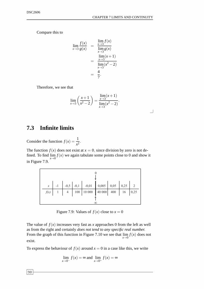
DSC2606
CHAPTER 7 LIMITS AND CONTINUITY
Compare this to
limx→3
f (x)g(x)
=limx→3
f (x)
limx→3
g(x)
=limx→3
(x+1)
limx→3
(x2−2)
=47.
Therefore, we see that
limx→3
(
x+1x2−2
)
=limx→3
(x+1)
limx→3
(x2−2).
7.3 Infinite limits
Consider the functionf (x) =1x2 .
The functionf (x) does not exist atx = 0, since division by zero is not de-fined. To find lim
x→0f (x) we again tabulate some points close to 0 and show it
in Figure 7.9.
x
f ( x )
- 1
1
- 0 , 5
4
- 0 , 1
1 0 0
- 0 , 0 1
1 0 0 0 0
0 , 0 0 5
4 0 0 0 0
0 , 0 5
4 0 0
0 , 2 5
1 6
2
0 , 2 5
0
¥
Figure 7.9: Values off (x) close tox= 0
The value off (x) increases very fast asx approaches 0 from the left as wellas from the right and certainlydoes not tend to any specific real number.From the graph of this function in Figure 7.10 we see that lim
x→0f (x) does not
exist.
To express the behaviour off (x) aroundx= 0 in a case like this, we write
limx→0−
f (x) = ∞ and limx→0+
f (x) = ∞
90
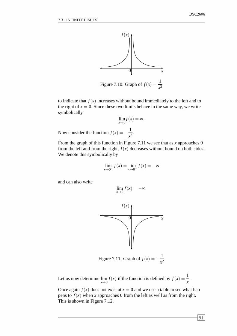
7.3. INFINITE LIMITS
DSC2606
x
f (x)
0
Figure 7.10: Graph off (x) =1x2
to indicate thatf (x) increases without bound immediately to the left and tothe right ofx = 0. Since these two limits behave in the same way, we writesymbolically
limx→0
f (x) = ∞.
Now consider the functionf (x) =− 1x2 .
From the graph of this function in Figure 7.11 we see that asx approaches 0from the left and from the right,f (x) decreases without bound on both sides.We denote this symbolically by
limx→0−
f (x) = limx→0+
f (x) =−∞
and can also writelimx→0
f (x) =−∞.
x
f (x)
0
Figure 7.11: Graph off (x) =− 1x2
Let us now determine limx→0
f (x) if the function is defined byf (x) =1x.
Once againf (x) does not exist atx= 0 and we use a table to see what hap-pens tof (x) whenx approaches 0 from the left as well as from the right.This is shown in Figure 7.12.
91

DSC2606
CHAPTER 7 LIMITS AND CONTINUITY
x
f ( x )
- 0 , 5
- 2
- 0 , 1
- 1 0
- 0 , 0 1
- 1 0 0
- 0 , 0 0 1
- 1 0 0 0
0 , 0 0 1
1 0 0 0
0 , 0 1
1 0 0
0 , 1
1 0
0 , 5
2
0
?
Figure 7.12: Values off (x) close tox= 0
We see that asx approaches 0 from the left, the value off (x) decreases with-out bound. This is written as
limx→0−
f (x) =−∞.
On the other hand, ifx approaches 0 from the right, the value off (x) in-creases without bound. We write this as
limx→0+
f (x) = +∞.
In this case, we can only say that limx→0
f (x) does not exist and no special nota-
tion applies. From the graph in Figure 7.13, we can see clearly that no limitexists ifx tends to 0.
x
f (x)
0
Figure 7.13: Graph off (x) =1x
7.4 Limits when x tends to infinity
In our discussion of limx→a
f (x) so far, we have considereda to be a real num-
ber. It is sometimes necessary to determine the behaviour ofa function when
92
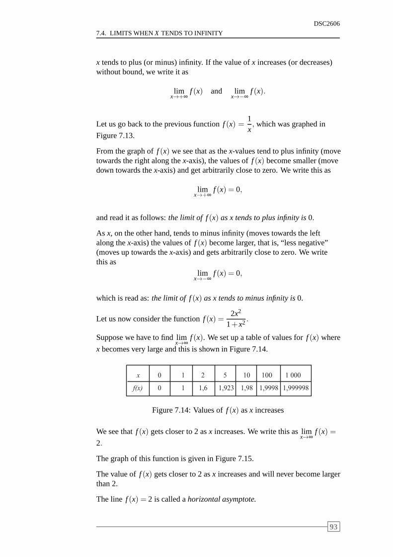
7.4. LIMITS WHENX TENDS TO INFINITY
DSC2606
x tends to plus (or minus) infinity. If the value ofx increases (or decreases)without bound, we write it as
limx→+∞
f (x) and limx→−∞
f (x).
Let us go back to the previous functionf (x) =1x, which was graphed in
Figure 7.13.
From the graph off (x) we see that as thex-values tend to plus infinity (movetowards the right along thex-axis), the values off (x) become smaller (movedown towards thex-axis) and get arbitrarily close to zero. We write this as
limx→+∞
f (x) = 0,
and read it as follows:the limit of f(x) as x tends to plus infinity is0.
As x, on the other hand, tends to minus infinity (moves towards theleftalong thex-axis) the values off (x) become larger, that is, “less negative”(moves up towards thex-axis) and gets arbitrarily close to zero. We writethis as
limx→−∞
f (x) = 0,
which is read as:the limit of f(x) as x tends to minus infinity is0.
Let us now consider the functionf (x) =2x2
1+x2 .
Suppose we have to find limx→∞
f (x). We set up a table of values forf (x) where
x becomes very large and this is shown in Figure 7.14.
x
f ( x )
0
0
1
1
2
1 , 6
5
1 , 9 2 3
1 0
1 , 9 8 1 , 9 9 9 8
1 0 0 0
1 , 9 9 9 9 9 8
1 0 0
Figure 7.14: Values off (x) asx increases
We see thatf (x) gets closer to 2 asx increases. We write this as limx→∞
f (x) =
2.
The graph of this function is given in Figure 7.15.
The value off (x) gets closer to 2 asx increases and will never become largerthan 2.
The line f (x) = 2 is called ahorizontal asymptote.
93
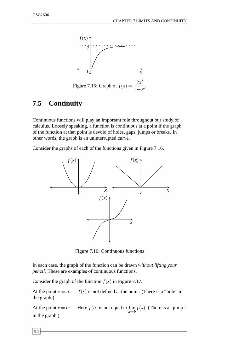
DSC2606
CHAPTER 7 LIMITS AND CONTINUITY
x
f (x)
2
0
Figure 7.15: Graph off (x) =2x2
1+x2
7.5 Continuity
Continuous functions will play an important role throughout our study ofcalculus. Loosely speaking, a function is continuous at a point if the graphof the function at that point is devoid of holes, gaps, jumps or breaks. Inother words, the graph is an uninterrupted curve.
Consider the graphs of each of the functions given in Figure 7.16.
x
f (x)
x
f (x)
x
f (x)
Figure 7.16: Continuous functions
In each case, the graph of the function can be drawnwithout lifting yourpencil.These are examples of continuous functions.
Consider the graph of the functionf (x) in Figure 7.17.
At the pointx = a: f (x) is not defined at the point. (There is a “hole” inthe graph.)
At the pointx= b: Here f (b) is not equal to limx→b
f (x). (There is a “jump ”
in the graph.)
94
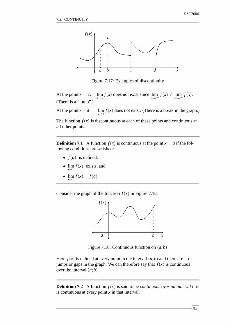
7.5. CONTINUITY
DSC2606
x
f (x)
bc
a
bc
b
bc
c d
b
Figure 7.17: Examples of discontinuity
At the pointx = c: limx→c
f (x) does not exist since limx→c−
f (x) 6= limx→c+
f (x).
(There is a “jump”.)
At the pointx=d: limx→d
f (x) does not exist. (There is a break in the graph.)
The functionf (x) is discontinuous at each of these points and continuous atall other points.
Definition 7.1 A function f (x) is continuous at the pointx = a if the fol-lowing conditions are satisfied:
• f (a) is defined,
• limx→a
f (x) exists, and
• limx→a
f (x) = f (a).
Consider the graph of the functionf (x) in Figure 7.18.
x
f (x)
a b
Figure 7.18: Continuous function on(a;b)
Here f (x) is defined at every point in the interval(a;b) and there are nojumps or gaps in the graph. We can therefore say thatf (x) is continuousover the interval(a;b).
Definition 7.2 A function f (x) is said to becontinuous over an intervalif itis continuous at every pointx in that interval.
95
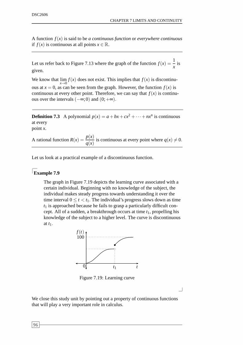
DSC2606
CHAPTER 7 LIMITS AND CONTINUITY
A function f (x) is said to bea continuous functionor everywhere continuousif f (x) is continuous at all pointsx∈ R.
Let us refer back to Figure 7.13 where the graph of the function f (x) =1x
is
given.
We know that limx→0
f (x) does not exist. This implies thatf (x) is discontinu-
ous atx= 0, as can be seen from the graph. However, the functionf (x) iscontinuous at every other point. Therefore, we can say thatf (x) is continu-ous over the intervals(−∞;0) and(0;+∞).
Definition 7.3 A polynomialp(x) = a+bx+cx2+ · · ·+nxn is continuousat everypointx.
A rational functionR(x) =p(x)q(x)
is continuous at every point whereq(x) 6= 0.
Let us look at a practical example of a discontinuous function.
Example 7.9
The graph in Figure 7.19 depicts the learning curve associated with acertain individual. Beginning with no knowledge of the subject, theindividual makes steady progress towards understanding itover thetime interval 0≤ t < t1. The individual’s progress slows down as timet1 is approached because he fails to grasp a particularly difficult con-cept. All of a sudden, a breakthrough occurs at timet1, propelling hisknowledge of the subject to a higher level. The curve is discontinuousat t1.
t
f (t)
t1
100
0
bbc
Figure 7.19: Learning curve
We close this study unit by pointing out a property of continuous functionsthat will play a very important role in calculus.
96
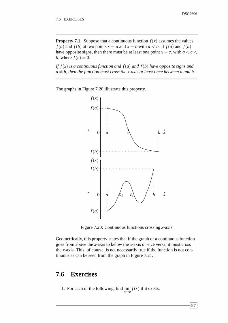
7.6. EXERCISES
DSC2606
Property 7.1 Suppose that a continuous functionf (x) assumes the valuesf (a) and f (b) at two pointsx = a andx = b with a < b. If f (a) and f (b)have opposite signs, then there must be at least one pointx= c, with a< c<b, where f (c) = 0.
If f (x) is a continuous function and f(a) and f(b) have opposite signs anda 6= b, then the function must cross the x-axis at least once between a and b.
The graphs in Figure 7.20 illustrate this property.
x
f (x)
f (a)
a
f (b)
b0 c
x
f (x)
f (a)
a
f (b)
b0 c1 c2
Figure 7.20: Continuous functions crossingx-axis
Geometrically, this property states that if the graph of a continuous functiongoes from above thex-axis to below thex-axis or vice versa, it must crossthex-axis. This, of course, is not necessarily true if the function is not con-tinuous as can be seen from the graph in Figure 7.21.
7.6 Exercises
1. For each of the following, find limx→a
f (x) if it exists:
97
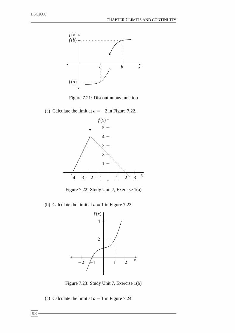
DSC2606
CHAPTER 7 LIMITS AND CONTINUITY
x
f (x)
f (a)
a
f (b)
b
b
bc
Figure 7.21: Discontinuous function
(a) Calculate the limit ata=−2 in Figure 7.22.
1
2
3
4
5
1 2 3−1−2−3−4x
f (x)
bc
b
Figure 7.22: Study Unit 7, Exercise 1(a)
(b) Calculate the limit ata= 1 in Figure 7.23.
2
4
1 2−1−2x
f (x)
Figure 7.23: Study Unit 7, Exercise 1(b)
(c) Calculate the limit ata= 1 in Figure 7.24.
98
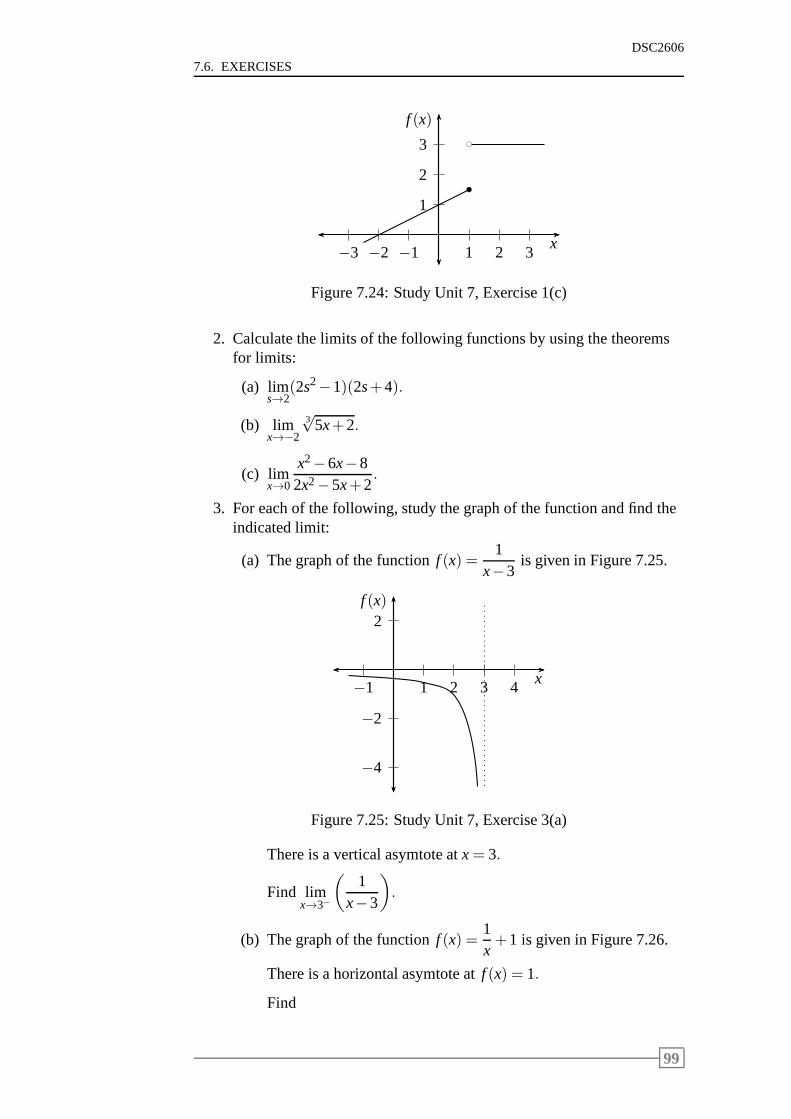
7.6. EXERCISES
DSC2606
1
2
3
1 2 3−1−2−3x
f (x)bc
b
Figure 7.24: Study Unit 7, Exercise 1(c)
2. Calculate the limits of the following functions by using the theoremsfor limits:
(a) lims→2
(2s2−1)(2s+4).
(b) limx→−2
3√
5x+2.
(c) limx→0
x2−6x−82x2−5x+2
.
3. For each of the following, study the graph of the function and find theindicated limit:
(a) The graph of the functionf (x) =1
x−3is given in Figure 7.25.
2
−2
−4
1 2 3 4−1x
f (x)
Figure 7.25: Study Unit 7, Exercise 3(a)
There is a vertical asymtote atx= 3.
Find limx→3−
(
1x−3
)
.
(b) The graph of the functionf (x) =1x+1 is given in Figure 7.26.
There is a horizontal asymtote atf (x) = 1.
Find
99
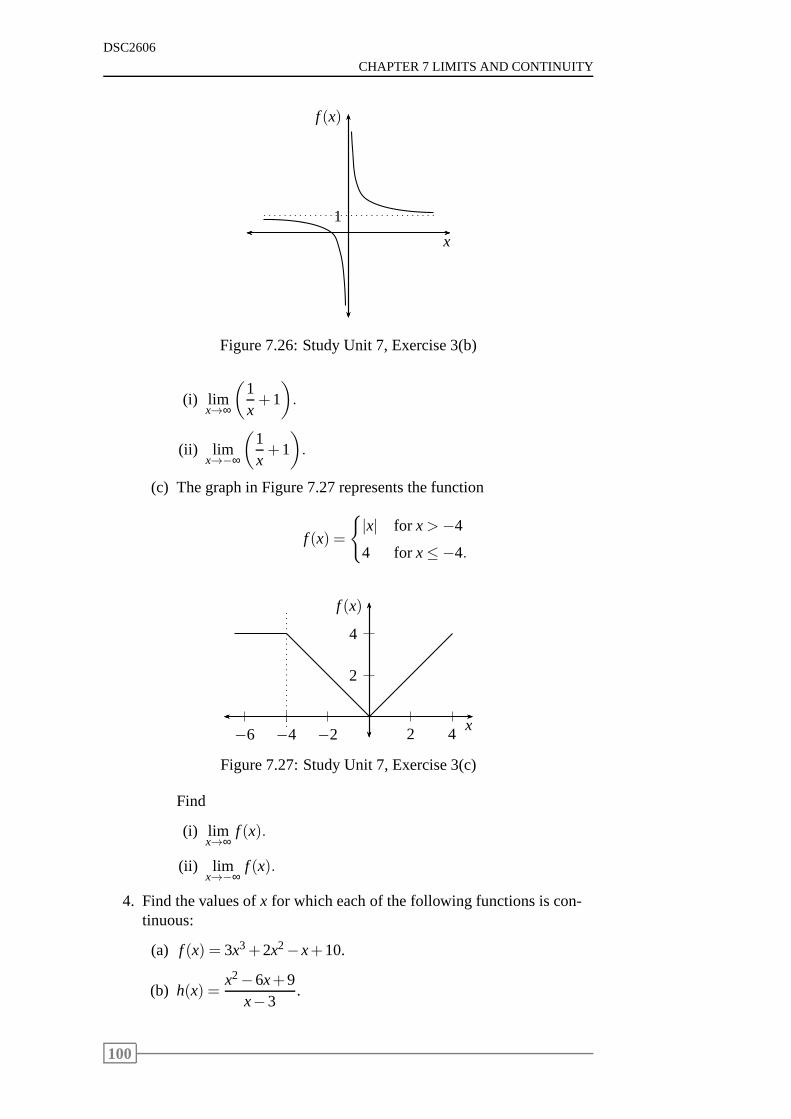
DSC2606
CHAPTER 7 LIMITS AND CONTINUITY
x
f (x)
1
Figure 7.26: Study Unit 7, Exercise 3(b)
(i) limx→∞
(
1x+1
)
.
(ii) limx→−∞
(
1x+1
)
.
(c) The graph in Figure 7.27 represents the function
f (x) =
{
|x| for x>−4
4 for x≤−4.
2
4
2 4−2−4−6x
f (x)
Figure 7.27: Study Unit 7, Exercise 3(c)
Find
(i) limx→∞
f (x).
(ii) limx→−∞
f (x).
4. Find the values ofx for which each of the following functions is con-tinuous:
(a) f (x) = 3x3+2x2−x+10.
(b) h(x) =x2−6x+9
x−3.
100
7.7. SOLUTIONS TO EXERCISES
DSC2606
5. Determine all the values ofx at which the following function is dis-continuous:
f (x) =x2−3x+2
x2−2x.
7.7 Solutions to exercises
1. (a) limx→−2
f (x) = 4.
(b) limx→1
f (x) = 2.
(c) limx→1
f (x) does not exist.
2. (a) The limit is
lims→2
(2s2−1)(2s+4) = lims→2
(2s2−1)× lims→2
(2s+4)
= (2 ·22−1)× (2 ·2+4)
= 7×8
= 56.
(b) The limit is
limx→−2
3√
5x+2 = limx→−2
(5x+2)13
= [ limx→−2
(5x+2)]13
= [5(−2)+2]13
= (−8)13
= −2.
(c) The limit is
limx→0
x2−6x−82x2−5x+2
=limx→0
(x2−6x−8)
limx→0
(2x2−5x+2)
=−82
= −4.
3. (a) limx→3−
(
1x−3
)
=−∞.
(b) (i) limx→∞
(
1x+1
)
= 1.
101
DSC2606
CHAPTER 7 LIMITS AND CONTINUITY
(ii) limx→−∞
(
1x+1
)
= 1.
(c) (i) limx→∞
f (x) = ∞.
(ii) limx→−∞
f (x) = 4.
4. (a) The functionf (x) is a polynomial function and is therefore con-tinuous for all values ofx.
(b) The functionh(x) is a rational function and is continuous at ev-ery point where the denominator,x−3 6= 0. The functionh(x) istherefore continuous everywhere except atx= 3.
5. The functionf (x) is discontinuous wherex2−2x= x(x−2) = 0, thatis, atx= 0 andx= 2.
102
Chapter 8
The derivative of a function
Contents8.1 Introduction . . . . . . . . . . . . . . . . . . . . . . . . 104
8.2 The slope of a tangent line . . . . . . . . . . . . . . . . . 106
8.3 The rate of change . . . . . . . . . . . . . . . . . . . . . 109
8.4 The derivative of a function . . . . . . . . . . . . . . . . 109
8.5 Differentiability and continuity . . . . . . . . . . . . . . 114
8.6 Exercises . . . . . . . . . . . . . . . . . . . . . . . . . . 115
8.7 Solutions to exercises . . . . . . . . . . . . . . . . . . . 117
103
DSC2606
CHAPTER 8 THE DERIVATIVE OF A FUNCTION
Learning objectives
After completing this study unit you should be able to
• explain the concept of a tangent line to the curve of a function
• explain the concept of the average rate of change of a function over aninterval
• explain the concept of the instantaneous rate of change of a function ata point
• explain the concept of the derivative of a function
• understand how the derivative of a function is evaluated by means of alimit
• understand the relationship between continuity and differentiability.
8.1 Introduction
The derivative of a function will be defined in this study unit. You mustunderstand the concepts discussed, but you will not be examined on thisstudy unit explicitly.
We will show that the derivative of a function is equal to the slope of thetangent line to the function. We mentioned in the previous study unit thatthe problem of finding therate of changeof one quantity with respect toanother is mathematically equivalent to finding theslope of the tangent lineto a curve at a given point on the curve. In other words, since the slope of atangent line and the derivative are the same thing, a rate of change problemcan be solved by finding the derivative of the function.
Before going on to define the derivative, let us show the relationship be-tween the rate of change and the slope of the tangent line by means of agraphical example.
Consider the speed of a car as given by the function
f (t) = 2t2 for t ≥ 0,
wheret represents time. The graph of this function is given in Figure 8.1.
104
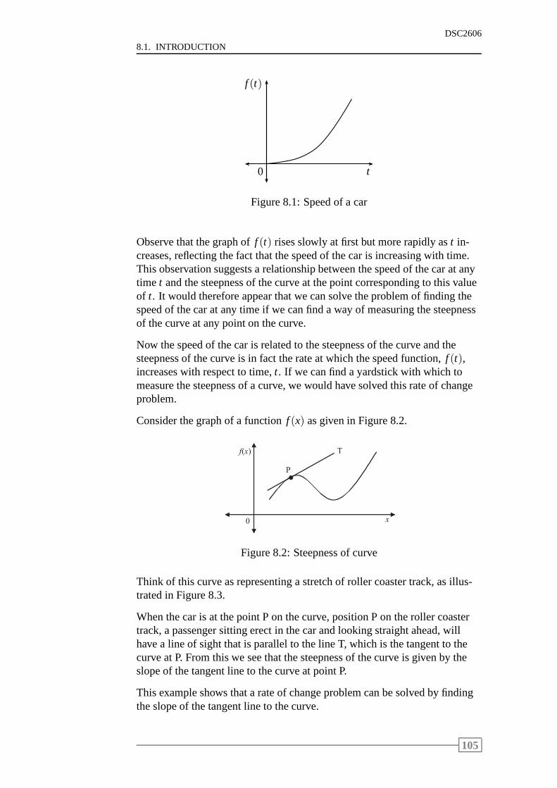
8.1. INTRODUCTION
DSC2606
t
f (t)
0
Figure 8.1: Speed of a car
Observe that the graph off (t) rises slowly at first but more rapidly ast in-creases, reflecting the fact that the speed of the car is increasing with time.This observation suggests a relationship between the speedof the car at anytime t and the steepness of the curve at the point corresponding to this valueof t. It would therefore appear that we can solve the problem of finding thespeed of the car at any time if we can find a way of measuring the steepnessof the curve at any point on the curve.
Now the speed of the car is related to the steepness of the curve and thesteepness of the curve is in fact the rate at which the speed function, f (t),increases with respect to time,t. If we can find a yardstick with which tomeasure the steepness of a curve, we would have solved this rate of changeproblem.
Consider the graph of a functionf (x) as given in Figure 8.2.
0
f ( x )
x
P
T
Figure 8.2: Steepness of curve
Think of this curve as representing a stretch of roller coaster track, as illus-trated in Figure 8.3.
When the car is at the point P on the curve, position P on the roller coastertrack, a passenger sitting erect in the car and looking straight ahead, willhave a line of sight that is parallel to the line T, which is thetangent to thecurve at P. From this we see that the steepness of the curve is given by theslope of the tangent line to the curve at point P.
This example shows that a rate of change problem can be solvedby findingthe slope of the tangent line to the curve.
105
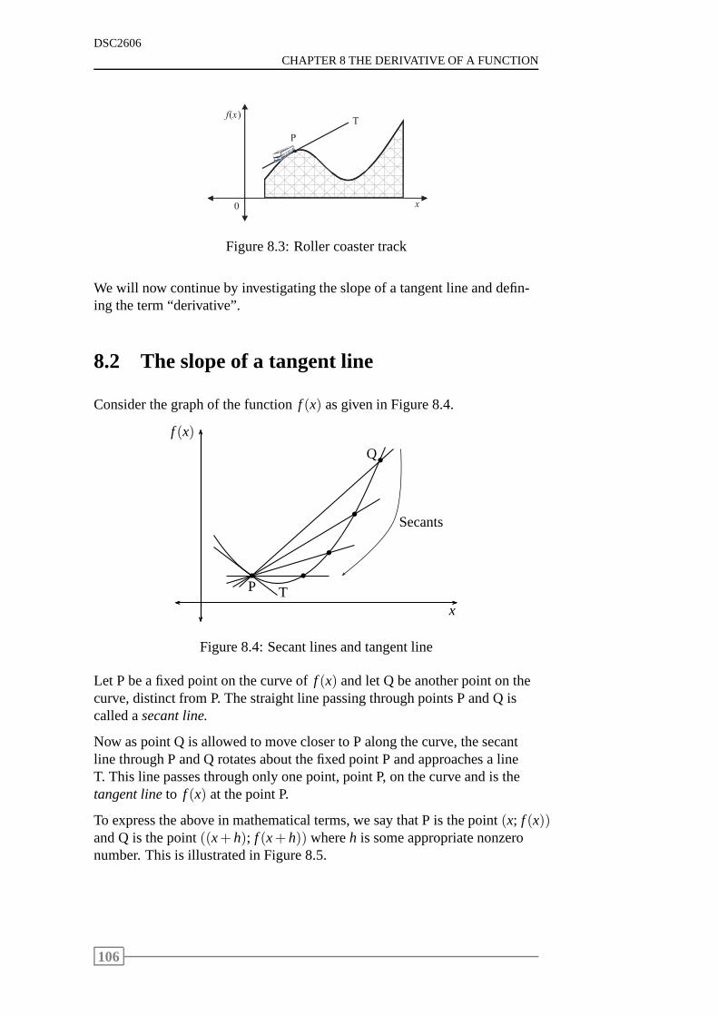
DSC2606
CHAPTER 8 THE DERIVATIVE OF A FUNCTION
0
f ( x )
x
T
P
Figure 8.3: Roller coaster track
We will now continue by investigating the slope of a tangent line and defin-ing the term “derivative”.
8.2 The slope of a tangent line
Consider the graph of the functionf (x) as given in Figure 8.4.
x
f (x)
b b
b
b
b
P
Q
T
Secants
Figure 8.4: Secant lines and tangent line
Let P be a fixed point on the curve off (x) and let Q be another point on thecurve, distinct from P. The straight line passing through points P and Q iscalled asecant line.
Now as point Q is allowed to move closer to P along the curve, the secantline through P and Q rotates about the fixed point P and approaches a lineT. This line passes through only one point, point P, on the curve and is thetangent lineto f (x) at the point P.
To express the above in mathematical terms, we say that P is the point(x; f (x))and Q is the point((x+h); f (x+h)) whereh is some appropriate nonzeronumber. This is illustrated in Figure 8.5.
106
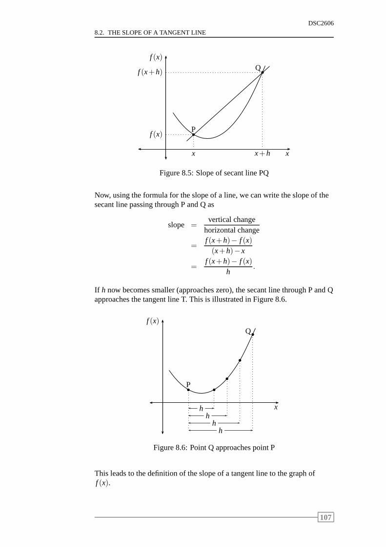
8.2. THE SLOPE OF A TANGENT LINE
DSC2606
x
f (x)
b
b
x
f (x)
x+h
f (x+h)
P
Q
Figure 8.5: Slope of secant line PQ
Now, using the formula for the slope of a line, we can write theslope of thesecant line passing through P and Q as
slope =vertical change
horizontal change
=f (x+h)− f (x)(x+h)−x
=f (x+h)− f (x)
h.
If h now becomes smaller (approaches zero), the secant line through P and Qapproaches the tangent line T. This is illustrated in Figure8.6.
x
f (x)
b b
b
b
b
hh
hh
P
Q
Figure 8.6: Point Q approaches point P
This leads to the definition of the slope of a tangent line to the graph off (x).
107

DSC2606
CHAPTER 8 THE DERIVATIVE OF A FUNCTION
Definition 8.1 Theslope of the tangent lineto the graphf (x) at the point(x; f (x)) is given by
limh→0
f (x+h)− f (x)h
,
if the limit exists.
108
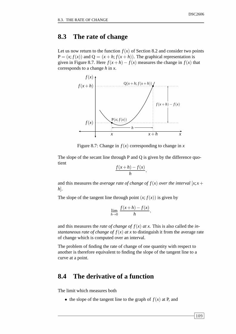
8.3. THE RATE OF CHANGE
DSC2606
8.3 The rate of change
Let us now return to the functionf (x) of Section 8.2 and consider two pointsP= (x; f (x)) and Q= (x+ h; f (x+ h)). The graphical representation isgiven in Figure 8.7. Heref (x+h)− f (x) measures the change inf (x) thatcorresponds to a changeh in x.
x
f (x)
b
b
x
f (x)h
x+h
f (x+h)
f (x+h)− f (x)
P(x; f (x))
Q(x+h; f (x+h))
Figure 8.7: Change inf (x) corresponding to change inx
The slope of the secant line through P and Q is given by the difference quo-tient
f (x+h)− f (x)h
,
and this measures theaverage rate of change of f(x) over the interval[x;x+h].
The slope of the tangent line through point(x; f (x)) is given by
limh→0
f (x+h)− f (x)h
,
and this measures therate of change of f(x) at x. This is also called thein-stantaneous rate of change of f(x) at x to distinguish it from the average rateof change which is computed over an interval.
The problem of finding the rate of change of one quantity with respect toanother is therefore equivalent to finding the slope of the tangent line to acurve at a point.
8.4 The derivative of a function
The limit which measures both
• the slope of the tangent line to the graph off (x) at P, and
109
DSC2606
CHAPTER 8 THE DERIVATIVE OF A FUNCTION
• the instantaneous rate of change off (x) at x,
is given a special name, namely thederivative of f(x) at x.
Definition 8.2 We define thederivative of a function f(x) with respect toxas the new function
f ′(x) = limh→0
f (x+h)− f (x)h
.
From these definitions it follows that the derivative of a function is equal tothe slope of the tangent line to the function.
Different notations are used for the derivative off (x) with respect tox.These notations are
• f ′(x) ( f prime x)
• dydx
(deey deex) if y= f (x)
• ddx
f (x) (dee deex of f (x)).
To calculate the derivative of a functionf (x), the following four steps areapplied:
Step 1: Calculatef (x+h).
Step 2: Calculate the differencef (x+h)− f (x).
Step 3: Calculate the quotientf (x+h)− f (x)
h.
Step 4: Calculatef ′(x) = limh→0
f (x+h)− f (x)h
.
We illustrate this by means of some examples.
Example 8.1
Find the slope of the tangent line to the graph off (x) = 3x+5 at anypoint (x; f (x)).
Solution
The slope of the tangent line to the graphf (x) at point(x; f (x)) is given bythe derivative off (x) atx. To find the derivative, we use the four-step pro-cess.
Step 1:
f (x+h) = 3(x+h)+5
= 3x+3h+5.
110
8.4. THE DERIVATIVE OF A FUNCTION
DSC2606
Step 2:
f (x+h)− f (x) = 3x+3h+5− (3x+5)
= 3h.
Step 3:
f (x+h)− f (x)h
=3hh
= 3.
Step 4:
f ′(x) = limh→0
f (x+h)− f (x)h
= limh→0
3
= 3.
We could have expected this result, since the tangent line toa straight lineat any point must coincide with the line itself and, therefore, must have thesame slope as the line. In this case, the graph off (x) is a straight line withslope 3.
Example 8.2
Consider the functionf (x) = x2−4x.
(a) Calculatef ′(x).
(b) Find the point on the graph off (x) where the tangent line to thecurve is horizontal.
(c) Sketch the graph off (x) and the tangent line to the curve at thepoint found in (b).
(d) What is the rate of change off (x) at the point found in (b)?
Solution
(a) To find f ′(x) we use the four-step process.
Step 1:
f (x+h) = (x+h)2−4(x+h)
= x2+2xh+h2−4x−4h.
Step 2:
f (x+h)− f (x) = x2+2xh+h2−4x−4h− (x2−4x)
= 2xh+h2−4h
= h(2x+h−4).
111
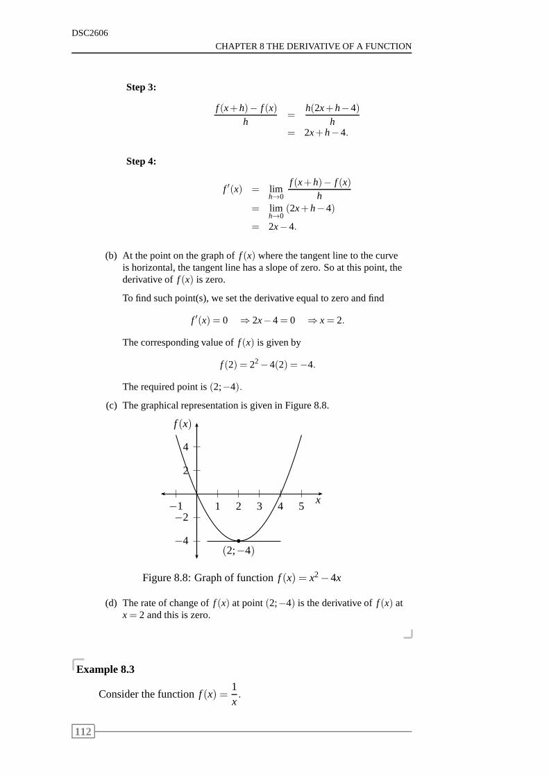
DSC2606
CHAPTER 8 THE DERIVATIVE OF A FUNCTION
Step 3:
f (x+h)− f (x)h
=h(2x+h−4)
h= 2x+h−4.
Step 4:
f ′(x) = limh→0
f (x+h)− f (x)h
= limh→0
(2x+h−4)
= 2x−4.
(b) At the point on the graph off (x) where the tangent line to the curveis horizontal, the tangent line has a slope of zero. So at thispoint, thederivative of f (x) is zero.
To find such point(s), we set the derivative equal to zero and find
f ′(x) = 0 ⇒ 2x−4= 0 ⇒ x= 2.
The corresponding value off (x) is given by
f (2) = 22−4(2) =−4.
The required point is(2;−4).
(c) The graphical representation is given in Figure 8.8.
2
4
−2
−4
1 2 3 4 5−1x
f (x)
b
(2;−4)
Figure 8.8: Graph of functionf (x) = x2−4x
(d) The rate of change off (x) at point(2;−4) is the derivative off (x) atx= 2 and this is zero.
Example 8.3
Consider the functionf (x) =1x.
112
8.4. THE DERIVATIVE OF A FUNCTION
DSC2606
(a) Calculatef ′(x).
(b) Find the slope of the tangent line to the graph off (x) at the pointx= 1.
(c) Find the equation of the tangent line at pointx= 1.
Solution
(a) Step 1:
f (x+h) =1
x+h.
Step 2:
f (x+h)− f (x) =1
x+h− 1
x
=x− (x+h)x(x+h)
=−h
x(x+h).
Step 3:
f (x+h)− f (x)h
=−h
x(x+h)· 1h
=−1
x(x+h).
Step 4:
f ′(x) = limh→0
f (x+h)− f (x)h
= limh→0
−1x(x+h)
= − 1x2 .
(b) The slope of the tangent line to the graph off (x) atx= 1 is
f ′(1) =− 112 =−1.
(c) The tangent line is a straight line. At pointx = 1 we havef (1) = 1.The tangent line therefore passes through the point(1;1).
From (b) we know that the slope of the tangent line is−1.
Now remember that if the slope of a straight line ism and the linepasses through a point(x1;y1) then
m=y−y1
x−x1.
113
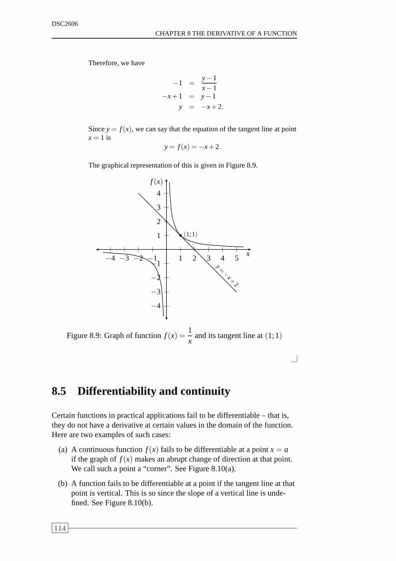
DSC2606
CHAPTER 8 THE DERIVATIVE OF A FUNCTION
Therefore, we have
−1 =y−1x−1
−x+1 = y−1
y = −x+2.
Sincey= f (x), we can say that the equation of the tangent line at pointx= 1 is
y= f (x) =−x+2.
The graphical representation of this is given in Figure 8.9.
1
2
3
4
−1
−2
−3
−4
1 2 3 4 5−1−2−3−4x
f (x)
y=−x+
2
b (1;1)
Figure 8.9: Graph of functionf (x) =1x
and its tangent line at(1;1)
8.5 Differentiability and continuity
Certain functions in practical applications fail to be differentiable – that is,they do not have a derivative at certain values in the domain of the function.Here are two examples of such cases:
(a) A continuous functionf (x) fails to be differentiable at a pointx = aif the graph off (x) makes an abrupt change of direction at that point.We call such a point a “corner”. See Figure 8.10(a).
(b) A function fails to be differentiable at a point if the tangent line at thatpoint is vertical. This is so since the slope of a vertical line is unde-fined. See Figure 8.10(b).
114
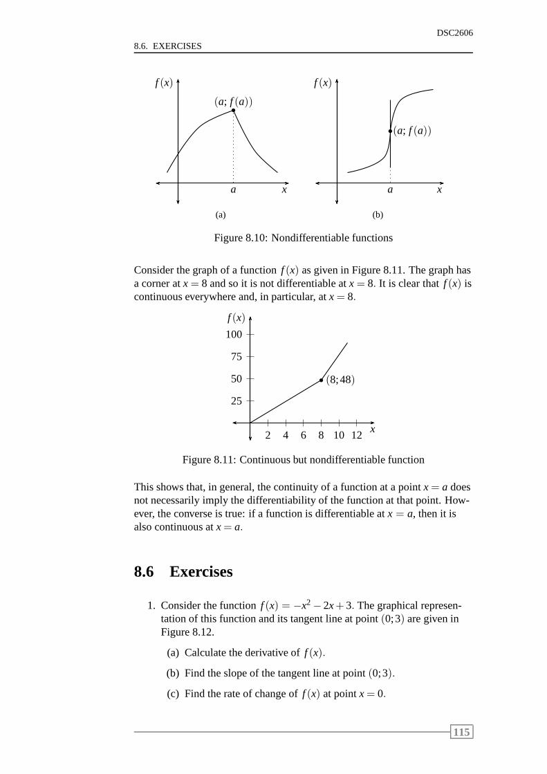
8.6. EXERCISES
DSC2606
x
f (x)
b(a; f (a))
a
(a)
x
f (x)
b (a; f (a))
a
(b)
Figure 8.10: Nondifferentiable functions
Consider the graph of a functionf (x) as given in Figure 8.11. The graph hasa corner atx= 8 and so it is not differentiable atx= 8. It is clear thatf (x) iscontinuous everywhere and, in particular, atx= 8.
25
50
75
100
2 4 6 8 10 12x
f (x)
b (8;48)
Figure 8.11: Continuous but nondifferentiable function
This shows that, in general, the continuity of a function at apointx= a doesnot necessarily imply the differentiability of the function at that point. How-ever, the converse is true: if a function is differentiable at x = a, then it isalso continuous atx= a.
8.6 Exercises
1. Consider the functionf (x) = −x2−2x+3. The graphical represen-tation of this function and its tangent line at point(0;3) are given inFigure 8.12.
(a) Calculate the derivative off (x).
(b) Find the slope of the tangent line at point(0;3).
(c) Find the rate of change off (x) at pointx= 0.
115
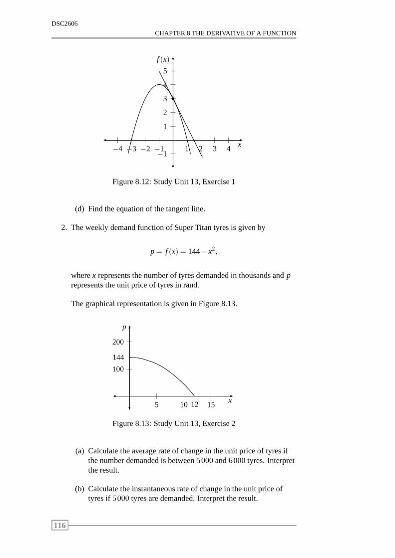
DSC2606
CHAPTER 8 THE DERIVATIVE OF A FUNCTION
1
2
3
4
5
−11 2 3 4−1−2−3−4
x
f (x)
b
Figure 8.12: Study Unit 13, Exercise 1
(d) Find the equation of the tangent line.
2. The weekly demand function of Super Titan tyres is given by
p= f (x) = 144−x2,
wherex represents the number of tyres demanded in thousands andprepresents the unit price of tyres in rand.
The graphical representation is given in Figure 8.13.
100
200
5 10 15x
p
144
12
Figure 8.13: Study Unit 13, Exercise 2
(a) Calculate the average rate of change in the unit price of tyres ifthe number demanded is between 5000 and 6000 tyres. Interpretthe result.
(b) Calculate the instantaneous rate of change in the unit price oftyres if 5000 tyres are demanded. Interpret the result.
116
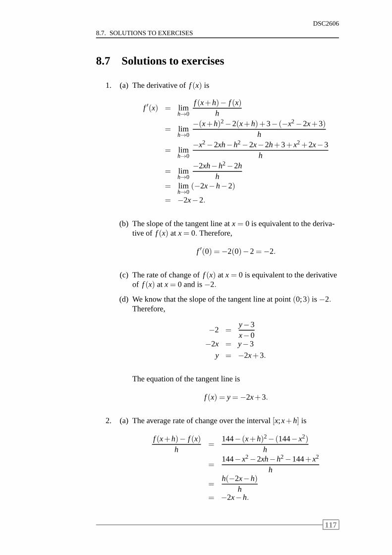
8.7. SOLUTIONS TO EXERCISES
DSC2606
8.7 Solutions to exercises
1. (a) The derivative off (x) is
f ′(x) = limh→0
f (x+h)− f (x)h
= limh→0
−(x+h)2−2(x+h)+3− (−x2−2x+3)h
= limh→0
−x2−2xh−h2−2x−2h+3+x2+2x−3h
= limh→0
−2xh−h2−2hh
= limh→0
(−2x−h−2)
= −2x−2.
(b) The slope of the tangent line atx= 0 is equivalent to the deriva-tive of f (x) at x= 0. Therefore,
f ′(0) =−2(0)−2=−2.
(c) The rate of change off (x) at x= 0 is equivalent to the derivativeof f (x) at x= 0 and is−2.
(d) We know that the slope of the tangent line at point(0;3) is−2.Therefore,
−2 =y−3x−0
−2x = y−3
y = −2x+3.
The equation of the tangent line is
f (x) = y=−2x+3.
2. (a) The average rate of change over the interval[x;x+h] is
f (x+h)− f (x)h
=144− (x+h)2− (144−x2)
h
=144−x2−2xh−h2−144+x2
h
=h(−2x−h)
h= −2x−h.
117
DSC2606
CHAPTER 8 THE DERIVATIVE OF A FUNCTION
This average rate of change must be calculated for a demand ofbetween 5000 and 6000 tyres. Therefore,x = 5 andx+h = 6,which means thath= 1.
Now the average rate of change if between 5000 and 6000 tyresare demanded is−2(5)−1=−11.
This means that the unit price decreases by R11 per thousandtyres if between 5000 and 6000 tyres are demanded.
(b) The instantaneous rate of change ifx tyres are demanded is
limh→0
f (x+h)− f (x)h
= limh→0
(−2x−h)
= −2x.
The instantaneous rate of change if 5000 tyres are demanded isthen−2(5) =−10.
This means that at the level where 5000 tyres are demanded, theunit price of a tyre is dropping at the rate of R10 per thousandtyres.
118
Chapter 9
The rules of differentiation
Contents9.1 Four basic rules . . . . . . . . . . . . . . . . . . . . . . 120
9.2 The product rule . . . . . . . . . . . . . . . . . . . . . . 125
9.3 The derivative of the exponential function . . . . . . . . 125
9.4 The derivative of the logarithmic function . . . . . . . . 126
9.5 Higher-order derivatives . . . . . . . . . . . . . . . . . 127
9.6 The chain rule . . . . . . . . . . . . . . . . . . . . . . . 128
9.7 Exercises . . . . . . . . . . . . . . . . . . . . . . . . . . 133
9.8 Solutions to exercises . . . . . . . . . . . . . . . . . . . 134
119
DSC2606
CHAPTER 9 THE RULES OF DIFFERENTIATION
Sections from prescribed book,WinstonChapter 11, Section 11.1
Learning objectivesAfter completing this study unit you should be able to
• calculate the derivatives of functions by applying the rules of differen-tiation
• use derivatives to solve rate of change problems.
9.1 Four basic rules
When we calculated the derivative of a function in the previous study unit,we based the method on a faithful interpretation of the definition of thederivative as the limit of a quotient. To find the derivativef ′(x) of a functionf (x), we first calculated the difference quotient
f (x+h)− f (x)h
,
and then evaluated its limit ash approached 0. As you probably observed,this method is tedious even for relatively simple functions.
The main purpose of this study unit is to give certain rules that will simplifythe process of finding the derivative of a function. We will use the notation
ddx
[ f (x)]
[read “dee, deex of f of x”] to mean “the derivative of the function withrespect tox”. In stating the rules of differentiation, we assume that the func-tions f (x) andg(x) are differentiable.
RuleDerivative of a constant
ddx
(c) = 0, wherec is a constant.
The derivative of a constant function is equal to zero.
120
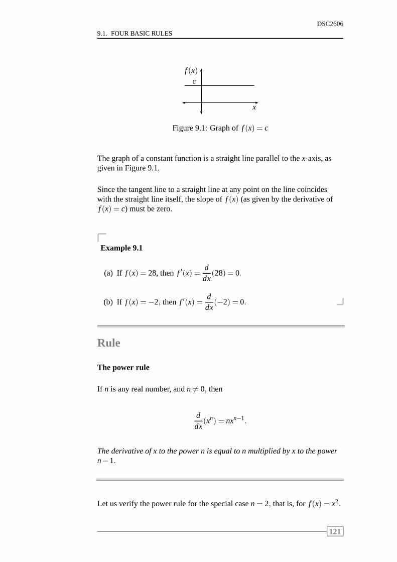
9.1. FOUR BASIC RULES
DSC2606
x
f (x)c
Figure 9.1: Graph off (x) = c
The graph of a constant function is a straight line parallel to thex-axis, asgiven in Figure 9.1.
Since the tangent line to a straight line at any point on the line coincideswith the straight line itself, the slope off (x) (as given by the derivative off (x) = c) must be zero.
Example 9.1
(a) If f (x) = 28, thenf ′(x) =ddx
(28) = 0.
(b) If f (x) =−2, then f ′(x) =ddx
(−2) = 0.
Rule
The power rule
If n is any real number, andn 6= 0, then
ddx
(xn) = nxn−1.
The derivative of x to the power n is equal to n multiplied by x to the powern−1.
Let us verify the power rule for the special casen= 2, that is, for f (x) = x2.
121
DSC2606
CHAPTER 9 THE RULES OF DIFFERENTIATION
The derivative is
f ′(x) = limh→0
f (x+h)− f (x)h
= limh→0
(x+h)2−x2
h
= limh→0
x2+2xh+h2−x2
h
= limh→0
2xh+h2
h= lim
h→0(2x+h)
= 2x.
Example 9.2
(a) If f (x) = x, then f ′(x) =ddx
(x) = 1x1−1 = x0 = 1.
(b) If f (x) = x8, then f ′(x) =ddx
(x8) = 8x8−1 = 8x7.
(c) If f (x) = x52 , then f ′(x) =
ddx
(x52) =
52
x52−1 =
52
x32 .
In order to differentiate functions containing radicals, like square roots, cuberoots, etc, we first rewrite the functions using fractional powers. These func-tions can then be differentiated using the power rule.
Example 9.3
(a) The functionf (x) =√
x can be rewritten asf (x) = x12 , and then
f ′(x) =ddx
(
x12
)
=12
x12−1 =
12
x−12 =
1
2x12
=1
2√
x.
(b) The functiong(x) =13√
xcan be rewritten asg(x) = x−
13 , and then
g′(x) =ddx
(
x−13
)
=−13
x−13−1 =−1
3x−
43 =− 1
3x43
.
RuleDerivative of a constant multiple of a function
ddx
c f(x) = cddx
f (x), wherec is a constant.
122

9.1. FOUR BASIC RULES
DSC2606
The derivative of a constant times a function is equal to the constant timesthe derivative of the function.
Example 9.4
(a) If f (x) = 5x3, then
f ′(x) =ddx
(5x3) = 5ddx
(x3) = 5(3x2) = 15x2.
(b) If f (x) =3√x, then rewriting this as 3x−
12 we have
f ′(x) =ddx
(3x−12) = 3(−1
2x−
32 ) =− 3
2x32
.
RuleThe sum/difference rule
ddx
[ f (x)±g(x)] =ddx
f (x)± ddx
g(x).
The derivative of the sum (or difference) of two differentiable functions isequal to the sum (or difference) of their derivatives.
This result may be extended to the sum and difference of any finite numberof differentiable functions.
Example 9.5
(a) If f (x) = 4x5+3x4−8x2+x+3, then
f ′(x) =ddx
(4x5+3x4−8x2+x+3)
=ddx
(4x5)+ddx
(3x4)− ddx
(8x2)+ddx
(x)+ddx
(3)
= 20x4+12x3−16x+1.
(b) If g(t) =t2
5+
5t3 , then rewriting
1t3 ast−3, we have
g′(t) =ddt
(
15
t2+5t−3)
=25
t−15t−4
=25
t− 15t4 .
123

DSC2606
CHAPTER 9 THE RULES OF DIFFERENTIATION
Here the independent variable ist instead ofx, so we differentiate withrespect tot.
124
9.2. THE PRODUCT RULE
DSC2606
9.2 The product rule
RuleThe product rule
ddx
[ f (x)g(x)] = f (x)g′(x)+g(x) f ′(x).
The derivative of the product of two functions is the first function times thederivative of the second plus the second function times the derivative of thefirst.
The product rule may be extended to the case involving the product of anyfinite number of differentiable functions.
Example 9.6
(a) If f (x) = (2x2−1)(x3+3) then, by using the product rule,
f ′(x) = (2x2−1)ddx
(x3+3)+(x3+3)ddx
(2x2−1)
= (2x2−1)(3x2)+(x3+3)(4x)
= 6x4−3x2+4x4+12x
= 10x4−3x2+12x.
(b) The functionf (x)= x3(√
x+1) can be rewritten asf (x)= x3(
x12 +1
)
and by the product rule,
f ′(x) = x3 ddx
(
x12 +1
)
+(
x12 +1
) ddx
(x3)
= x3(
12
x−12
)
+(
x12 +1
)
(3x2)
=12
x52 +3x
52 +3x2
=72
x52 +3x2.
9.3 The derivative of the exponential function
To analyse mathematical models involving exponential and logarithmicfunctions in greater detail, we need to develop rules for calculating the deriva-tive of these functions.
125
DSC2606
CHAPTER 9 THE RULES OF DIFFERENTIATION
Rule
Derivative of the exponential function
ddx
(ex) = ex.
The derivative of the exponential function is equal to the function itself.
Example 9.7
If f (x) = x2ex, then by the product rule
f ′(x) = x2 ddx
(ex)+ex ddx
(x2)
= x2ex+ex(2x)
= xex(x+2).
9.4 The derivative of the logarithmic function
Rule
Derivative of lnxddx
(lnx) =1x
for x> 0.
The derivative of theln of x is equal to one over x.
.
Example 9.8
If f (x) = xlnx, then by the product rule
f ′(x) = xddx
(lnx)+(lnx)ddx
(x)
= x
(
1x
)
+ lnx
= 1+ lnx.
126

9.5. HIGHER-ORDER DERIVATIVES
DSC2606
9.5 Higher-order derivatives
The derivativef ′(x) of a function f (x) is also a function. As such, the dif-ferentiability of f ′(x) may be considered. Therefore, the functionf ′(x) has aderivative f ′′(x) at a pointx in the domain off ′(x) if the limit of the quotient
f ′(x+h)− f ′(x)h
exists ash approaches 0. In other words,f ′′(x) is the derivative of the firstderivative.
The functionf ′′(x) obtained in this manner is called the second derivative ofthe functionf (x), just as the derivativef ′(x) is often called the first deriva-tive of f (x). Continuing in this fashion, we are led to considering the third,fourth, and higher-order derivatives off (x) whenever they exist.
Notations for the first, second, third, and, in general,n-th derivatives of afunction f (x) at a pointx are f ′(x), f ′′(x), f ′′′(x), . . . , f (n)(x) respectively.
If f (x) is written in the formy = f (x), then the notation for its derivativesare
dydx
,d2ydx2 ,
d3ydx3 , . . . ,
dnydxn .
Example 9.9
The derivatives of all orders of the polynomial function
f (x) = x5−3x4+4x3−2x2+x−8,
are as follows:
f ′(x) = 5x4−12x3+12x2−4x+1,
f ′′(x) =ddx
f ′(x) = 20x3−36x2+24x−4,
f ′′′(x) =ddx
f ′′(x) = 60x2−72x+24,
f (4)(x) =ddx
f ′′′(x) = 120x−72,
f (5)(x) =ddx
f (4)(x) = 120,
f (n)(x) = 0 for all n> 5.
Example 9.10
127
DSC2606
CHAPTER 9 THE RULES OF DIFFERENTIATION
To find the third derivative of the functionf (x) = x23 , we proceed as
follows:
f ′(x) =23
x−13
f ′′(x) =ddx
f ′(x)
=23(−1
3)x−
43
= −29
x−43 ,
and the required derivative is then
f ′′′(x) =
(
−29
)(
−43
)
x−73 =
827
x−73 .
Just as the derivative of a functionf (x) at a pointx measures the rate ofchange of the function at that point, the second derivative of f (x) (the deriva-tive of f ′(x)) measures the rate of change of the derivativef ′(x) of the func-tion f (x). The third derivative of the functionf ′′′(x), measures the rate ofchange off ′′(x), and so on.
9.6 The chain rule
Consider the functionk(x) = (x2 + x+ 1)2. If we were to computek′(x)using only the rules of differentiation from the previous sections, then ourapproach might be to expandk(x). Therefore,
k(x) = (x2+x+1)2 = (x2+x+1)(x2+x+1) = x4+2x3+3x2+2x+1,
from which we findk′(x) = 4x3+6x2+6x+2.
But what about the functionH(x) = (x2 + x+ 1)100? The same techniquemay be used to find the derivative of the functionH(x), but the amount ofwork involved in this case would be prodigious!
Consider also the functionG(x) =√
x2+1. For each of the two functionsH(x) andG(x), the rules of differentiation cannot be applied directly to cal-culate the derivativesH ′(x) andG′(x).
Observe that bothH(x) andG(x) are composite functions; that is, each iscomposed of, or build up of, simpler functions.
Let us consider the functionH(x) = (x2+x+1)100.
128

9.6. THE CHAIN RULE
DSC2606
If we let u= f (x) = x2+x+1 andy= g(u) = u100, then
H(x) = (x2+x+1)100
= [ f (x)]100
= u100
= g(u).
And we can say thatH(x) is composed of two functions, namelyf (x) andg(u), or equivalentlyH(x) is composed of two functionsu andy.
Now consider the functionG(x) =√
x2+1.
If we let u= f (x) = x2+1 andy= g(u) =√
u, then
G(x) =√
x2+1
=√
f (x)
=√
u
= g(u).
And G(x) is composed of the two functionsf (x) andg(u), or equivalentlythe functionsu andy.
We now consider a general composite function
y= h(x) = g[ f (x)],
which can also be represented as
y= g(u) andu= f (x).
We now want to determine the derivative of this composite function. Sincethe composite functionh(x) is composed of two functionsy = g(u) andu = f (x), we suspect that the derivative ofh(x), h′(x), will be given by an
expression that involves the derivative ofy with respect tou,dydu
= g′(u),
and the derivative ofu with respect tox,dudx
= f ′(x). But how do we com-
bine these derivatives to find the derivative ofh(x)?
This question can be answered by the fact that the derivativeof each func-tion represents the rate of change of that function.
For example, suppose thaty= g(u) changes twice as fast asu, that is
g′(u) =dydu
= 2.
And thatu= f (x) changes three times faster thanx, that is
f ′(x) =dudx
= 3.
129

DSC2606
CHAPTER 9 THE RULES OF DIFFERENTIATION
Then we would expecty= h(x) to change six times faster thanx, that is
h′(x) = g′(u) f ′(x) = 2×3= 6,
or equivalentlydydx
=dydu× du
dx.
This observation suggests the following result:
RuleThe chain rule
If h(x) = g[ f (x)], then
h′(x) =ddx
g[ f (x)] = g′[ f (x)] f ′(x).
Equivalently, if we writeh(x) asy= g(u), whereu= f (x), then
dydx
=dydu× du
dx.
The derivative of a composite function is equal to the derivative of the outerfunction with respect to the inner function multiplied by the derivative of theinner function, where
inner function
↑g[ f (x)].
↓outer function
Many composite functionsh(x) = g[ f (x)] have the special form whereg is afunction to the powern andn is a real number; that is
h(x) = [ f (x)]n.
In other words, the functionh(x) is given by the power of a functionf (x).
The functions
k(x) = (x2+x+1)2, H(x) = (x2+x+1)100, G(x) =√
x2+1
are examples of this type of composite function. By using thefollowingcorollary of the chain rule, we are able to find the derivativeof this type offunction much more easily than by using the chain rule directly:
130
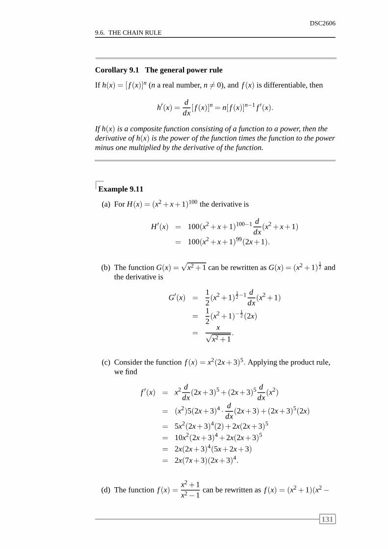
9.6. THE CHAIN RULE
DSC2606
Corollary 9.1 The general power rule
If h(x) = [ f (x)]n (n a real number,n 6= 0), and f (x) is differentiable, then
h′(x) =ddx
[ f (x)]n = n[ f (x)]n−1 f ′(x).
If h(x) is a composite function consisting of a function to a power, then thederivative of h(x) is the power of the function times the function to the powerminus one multiplied by the derivative of the function.
Example 9.11
(a) ForH(x) = (x2+x+1)100 the derivative is
H ′(x) = 100(x2+x+1)100−1 ddx
(x2+x+1)
= 100(x2+x+1)99(2x+1).
(b) The functionG(x) =√
x2+1 can be rewritten asG(x) = (x2+1)12 and
the derivative is
G′(x) =12(x2+1)
12−1 d
dx(x2+1)
=12(x2+1)−
12 (2x)
=x√
x2+1.
(c) Consider the functionf (x) = x2(2x+3)5. Applying the product rule,we find
f ′(x) = x2 ddx
(2x+3)5+(2x+3)5 ddx
(x2)
= (x2)5(2x+3)4 · ddx
(2x+3)+(2x+3)5(2x)
= 5x2(2x+3)4(2)+2x(2x+3)5
= 10x2(2x+3)4+2x(2x+3)5
= 2x(2x+3)4(5x+2x+3)
= 2x(7x+3)(2x+3)4.
(d) The functionf (x) =x2+1x2−1
can be rewritten asf (x) = (x2+1)(x2−
131
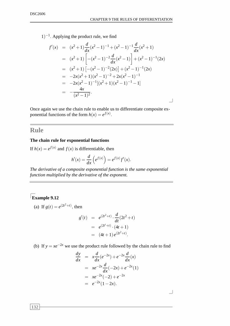
DSC2606
CHAPTER 9 THE RULES OF DIFFERENTIATION
1)−1. Applying the product rule, we find
f ′(x) = (x2+1)ddx
(x2−1)−1+(x2−1)−1 ddx
(x2+1)
= (x2+1)
[
−(x2−1)−2 ddx
(x2−1)
]
+(x2−1)−1(2x)
= (x2+1)[
−(x2−1)−2(2x)]
+(x2−1)−1(2x)
= −2x(x2+1)(x2−1)−2+2x(x2−1)−1
= −2x(x2−1)−1[(x2+1)(x2−1)−1−1]
= − 4x(x2−1)2 .
Once again we use the chain rule to enable us to differentiatecomposite ex-ponential functions of the formh(x) = ef (x).
RuleThe chain rule for exponential functions
If h(x) = ef (x) and f (x) is differentiable, then
h′(x) =ddx
(
ef (x))
= ef (x) f ′(x).
The derivative of a composite exponential function is the same exponentialfunction multiplied by the derivative of the exponent.
Example 9.12
(a) If g(t) = e(2t2+t), then
g′(t) = e(2t2+t) · ddt(2t2+ t)
= e(2tt+t) · (4t +1)
= (4t +1)e(2t2+t).
(b) If y= xe−2x we use the product rule followed by the chain rule to find
dydx
= xddx
(e−2x)+e−2x ddx
(x)
= xe−2x ddx
(−2x)+e−2x(1)
= xe−2x(−2)+e−2x
= e−2x(1−2x).
132
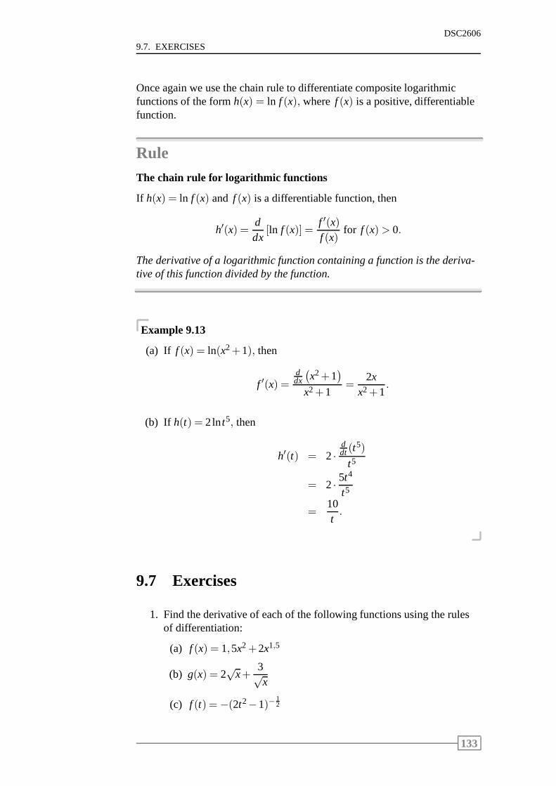
9.7. EXERCISES
DSC2606
Once again we use the chain rule to differentiate composite logarithmicfunctions of the formh(x) = ln f (x), where f (x) is a positive, differentiablefunction.
RuleThe chain rule for logarithmic functions
If h(x) = ln f (x) and f (x) is a differentiable function, then
h′(x) =ddx
[ln f (x)] =f ′(x)f (x)
for f (x)> 0.
The derivative of a logarithmic function containing a function is the deriva-tive of this function divided by the function.
Example 9.13
(a) If f (x) = ln(x2+1), then
f ′(x) =ddx
(
x2+1)
x2+1=
2xx2+1
.
(b) If h(t) = 2lnt5, then
h′(t) = 2 ·ddt(t
5)
t5
= 2 · 5t4
t5
=10t.
9.7 Exercises
1. Find the derivative of each of the following functions using the rulesof differentiation:
(a) f (x) = 1,5x2+2x1,5
(b) g(x) = 2√
x+3√x
(c) f (t) =−(2t2−1)−12
133
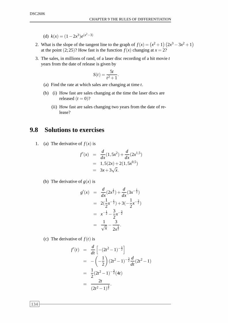
DSC2606
CHAPTER 9 THE RULES OF DIFFERENTIATION
(d) k(x) = (1−2x3)e(x2−3)
2. What is the slope of the tangent line to the graph off (x)=(
x2+1)(
2x3−3x2+1)
at the point(2;25)? How fast is the functionf (x) changing atx= 2?
3. The sales, in millions of rand, of a laser disc recording ofa hit movietyears from the date of release is given by
S(t) =5t
t2+1.
(a) Find the rate at which sales are changing at timet.
(b) (i) How fast are sales changing at the time the laser discsarereleased(t = 0)?
(ii) How fast are sales changing two years from the date of re-lease?
9.8 Solutions to exercises
1. (a) The derivative off (x) is
f ′(x) =ddx
(1,5x2)+ddx
(2x1,5)
= 1,5(2x)+2(1,5x0,5)
= 3x+3√
x.
(b) The derivative ofg(x) is
g′(x) =ddx
(2x12 )+
ddx
(3x−12)
= 2(12
x−12)+3(−1
2x−
32)
= x−12 − 3
2x−
32
=1√x− 3
2x32
.
(c) The derivative off (t) is
f ′(t) =ddt
[
−(2t2−1)−12
]
= −(
−12
)
(2t2−1)−32
ddt(2t2−1)
=12(2t2−1)−
32(4t)
=2t
(2t2−1)32
.
134
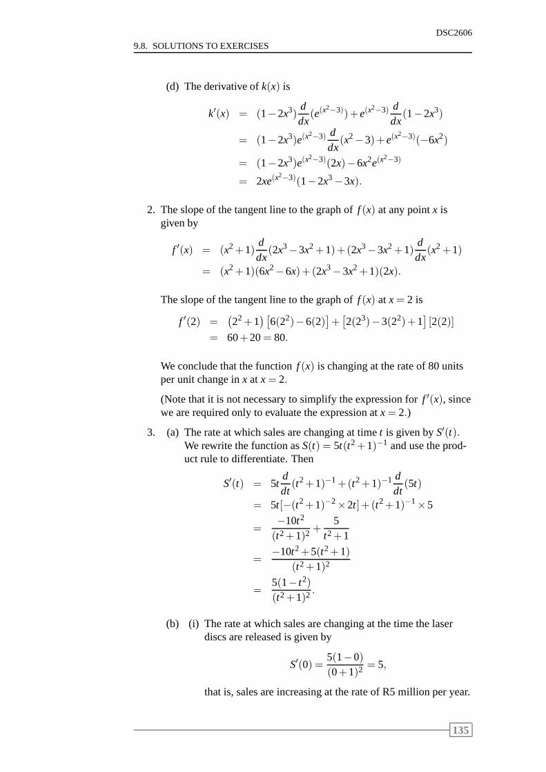
9.8. SOLUTIONS TO EXERCISES
DSC2606
(d) The derivative ofk(x) is
k′(x) = (1−2x3)ddx
(e(x2−3))+e(x
2−3) ddx
(1−2x3)
= (1−2x3)e(x2−3) d
dx(x2−3)+e(x
2−3)(−6x2)
= (1−2x3)e(x2−3)(2x)−6x2e(x
2−3)
= 2xe(x2−3)(1−2x3−3x).
2. The slope of the tangent line to the graph off (x) at any pointx isgiven by
f ′(x) = (x2+1)ddx
(2x3−3x2+1)+(2x3−3x2+1)ddx
(x2+1)
= (x2+1)(6x2−6x)+(2x3−3x2+1)(2x).
The slope of the tangent line to the graph off (x) at x= 2 is
f ′(2) =(
22+1)[
6(22)−6(2)]
+[
2(23)−3(22)+1]
[2(2)]
= 60+20= 80.
We conclude that the functionf (x) is changing at the rate of 80 unitsper unit change inx at x= 2.
(Note that it is not necessary to simplify the expression forf ′(x), sincewe are required only to evaluate the expression atx= 2.)
3. (a) The rate at which sales are changing at timet is given byS′(t).We rewrite the function asS(t) = 5t(t2+1)−1 and use the prod-uct rule to differentiate. Then
S′(t) = 5tddt(t2+1)−1+(t2+1)−1 d
dt(5t)
= 5t[−(t2+1)−2×2t]+(t2+1)−1×5
=−10t2
(t2+1)2 +5
t2+1
=−10t2+5(t2+1)
(t2+1)2
=5(1− t2)
(t2+1)2 .
(b) (i) The rate at which sales are changing at the time the laserdiscs are released is given by
S′(0) =5(1−0)(0+1)2 = 5,
that is, sales are increasing at the rate of R5 million per year.
135

DSC2606
CHAPTER 9 THE RULES OF DIFFERENTIATION
(ii) Two years from the date of release, sales are changing attherate of
S′(2) =5(1−4)(4+1)2 =−3
5=−0,6,
that is, decreasing at the rate of R600000 per year.
136
Chapter 10
Properties of functions andsketching graphs
Contents10.1 Introduction . . . . . . . . . . . . . . . . . . . . . . . . 138
10.2 Increasing and decreasing functions . . . . . . . . . . . 138
10.3 Relative and absolute extrema . . . . . . . . . . . . . . 141
10.4 Concavity . . . . . . . . . . . . . . . . . . . . . . . . . . 148
10.5 The second derivative test . . . . . . . . . . . . . . . . . 152
10.6 Asymptotes . . . . . . . . . . . . . . . . . . . . . . . . . 154
10.7 Sketching graphs . . . . . . . . . . . . . . . . . . . . . . 157
10.8 Exercises . . . . . . . . . . . . . . . . . . . . . . . . . . 160
10.9 Solutions to exercises . . . . . . . . . . . . . . . . . . . 161
137
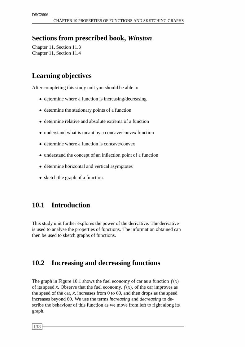
DSC2606
CHAPTER 10 PROPERTIES OF FUNCTIONS AND SKETCHING GRAPHS
Sections from prescribed book,WinstonChapter 11, Section 11.3Chapter 11, Section 11.4
Learning objectives
After completing this study unit you should be able to
• determine where a function is increasing/decreasing
• determine the stationary points of a function
• determine relative and absolute extrema of a function
• understand what is meant by a concave/convex function
• determine where a function is concave/convex
• understand the concept of an inflection point of a function
• determine horizontal and vertical asymptotes
• sketch the graph of a function.
10.1 Introduction
This study unit further explores the power of the derivative. The derivativeis used to analyse the properties of functions. The information obtained canthen be used to sketch graphs of functions.
10.2 Increasing and decreasing functions
The graph in Figure 10.1 shows the fuel economy of car as a function f (x)of its speedx. Observe that the fuel economy,f (x), of the car improves asthe speed of the car,x, increases from 0 to 60, and then drops as the speedincreases beyond 60. We use the termsincreasinganddecreasingto de-scribe the behaviour of this function as we move from left to right along itsgraph.
138
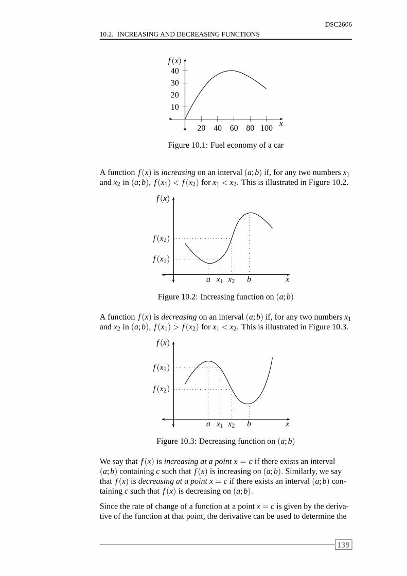
10.2. INCREASING AND DECREASING FUNCTIONS
DSC2606
10
20
30
40
20 40 60 80 100x
f (x)
Figure 10.1: Fuel economy of a car
A function f (x) is increasingon an interval(a;b) if, for any two numbersx1
andx2 in (a;b), f (x1)< f (x2) for x1 < x2. This is illustrated in Figure 10.2.
x
f (x)
a bx1
f (x1)
x2
f (x2)
Figure 10.2: Increasing function on(a;b)
A function f (x) is decreasingon an interval(a;b) if, for any two numbersx1
andx2 in (a;b), f (x1)> f (x2) for x1 < x2. This is illustrated in Figure 10.3.
x
f (x)
a bx1
f (x1)
x2
f (x2)
Figure 10.3: Decreasing function on(a;b)
We say thatf (x) is increasing at a point x= c if there exists an interval(a;b) containingc such thatf (x) is increasing on(a;b). Similarly, we saythat f (x) is decreasing at a point x= c if there exists an interval(a;b) con-tainingc such thatf (x) is decreasing on(a;b).
Since the rate of change of a function at a pointx= c is given by the deriva-tive of the function at that point, the derivative can be usedto determine the
139
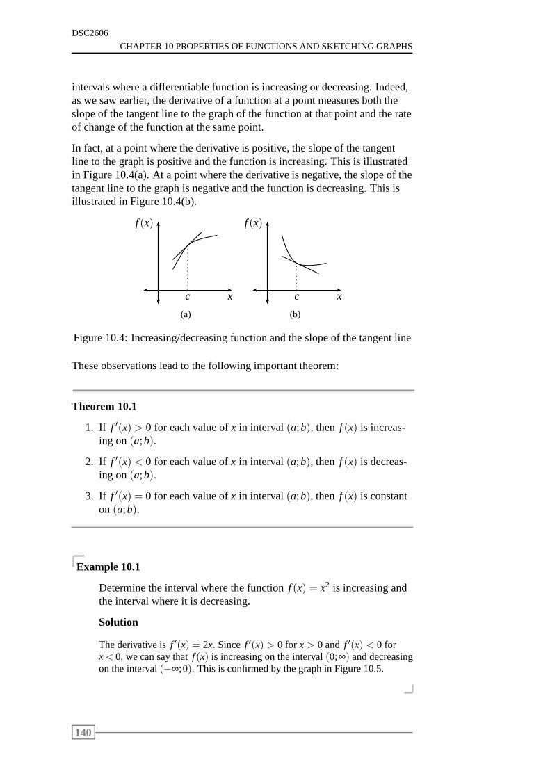
DSC2606
CHAPTER 10 PROPERTIES OF FUNCTIONS AND SKETCHING GRAPHS
intervals where a differentiable function is increasing ordecreasing. Indeed,as we saw earlier, the derivative of a function at a point measures both theslope of the tangent line to the graph of the function at that point and the rateof change of the function at the same point.
In fact, at a point where the derivative is positive, the slope of the tangentline to the graph is positive and the function is increasing.This is illustratedin Figure 10.4(a). At a point where the derivative is negative, the slope of thetangent line to the graph is negative and the function is decreasing. This isillustrated in Figure 10.4(b).
x
f (x)
c
(a)
x
f (x)
c
(b)
Figure 10.4: Increasing/decreasing function and the slopeof the tangent line
These observations lead to the following important theorem:
Theorem 10.1
1. If f ′(x) > 0 for each value ofx in interval(a;b), then f (x) is increas-ing on(a;b).
2. If f ′(x) < 0 for each value ofx in interval(a;b), then f (x) is decreas-ing on(a;b).
3. If f ′(x) = 0 for each value ofx in interval(a;b), then f (x) is constanton (a;b).
Example 10.1
Determine the interval where the functionf (x) = x2 is increasing andthe interval where it is decreasing.
Solution
The derivative isf ′(x) = 2x. Since f ′(x) > 0 for x > 0 and f ′(x) < 0 forx< 0, we can say thatf (x) is increasing on the interval(0;∞) and decreasingon the interval(−∞;0). This is confirmed by the graph in Figure 10.5.
140
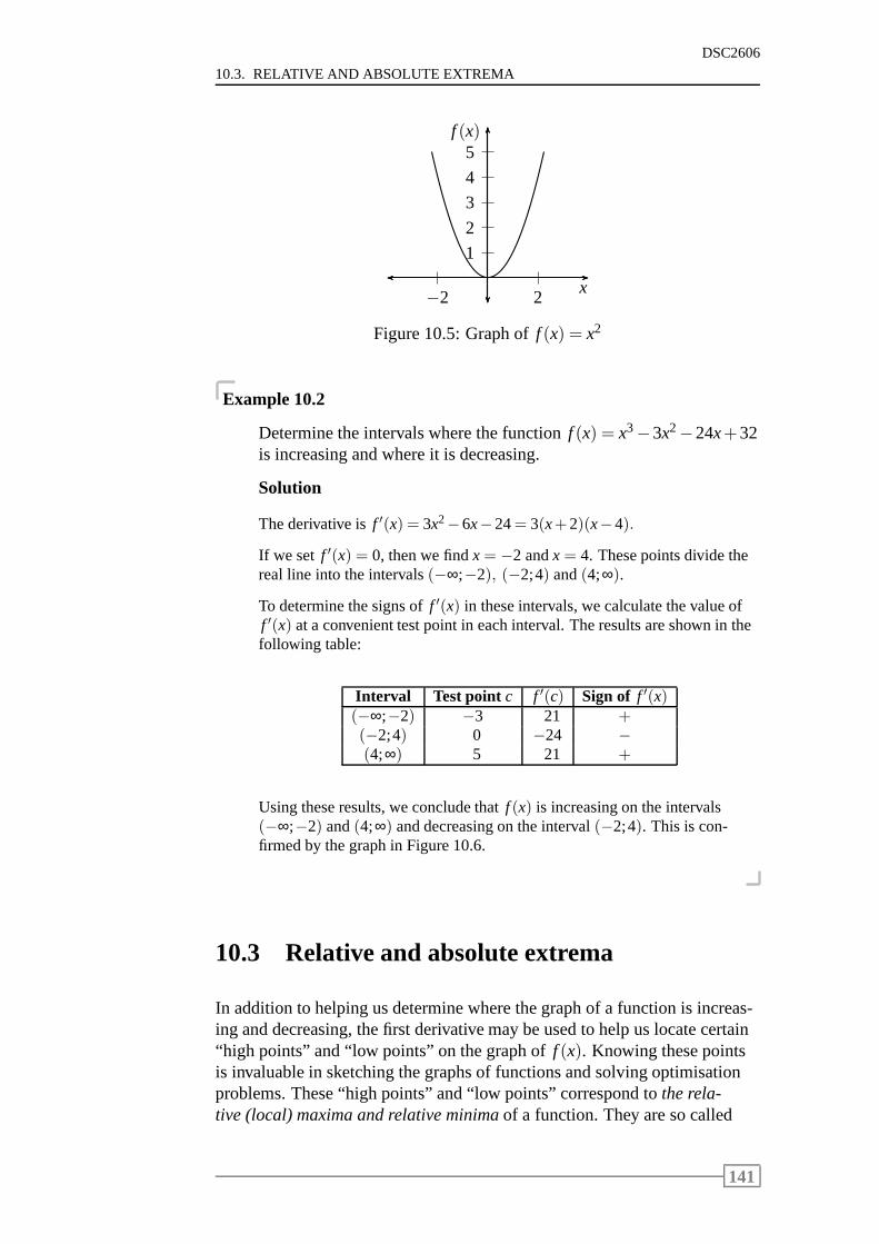
10.3. RELATIVE AND ABSOLUTE EXTREMA
DSC2606
1
2
3
4
5
2−2x
f (x)
Figure 10.5: Graph off (x) = x2
Example 10.2
Determine the intervals where the functionf (x) = x3−3x2−24x+32is increasing and where it is decreasing.
Solution
The derivative isf ′(x) = 3x2−6x−24= 3(x+2)(x−4).
If we set f ′(x) = 0, then we findx= −2 andx = 4. These points divide thereal line into the intervals(−∞;−2), (−2;4) and(4;∞).
To determine the signs off ′(x) in these intervals, we calculate the value off ′(x) at a convenient test point in each interval. The results are shown in thefollowing table:
Interval Test point c f ′(c) Sign of f ′(x)(−∞;−2) −3 21 +(−2;4) 0 −24 −(4;∞) 5 21 +
Using these results, we conclude thatf (x) is increasing on the intervals(−∞;−2) and(4;∞) and decreasing on the interval(−2;4). This is con-firmed by the graph in Figure 10.6.
10.3 Relative and absolute extrema
In addition to helping us determine where the graph of a function is increas-ing and decreasing, the first derivative may be used to help uslocate certain“high points” and “low points” on the graph off (x). Knowing these pointsis invaluable in sketching the graphs of functions and solving optimisationproblems. These “high points” and “low points” correspond to the rela-tive (local) maxima and relative minimaof a function. They are so called
141
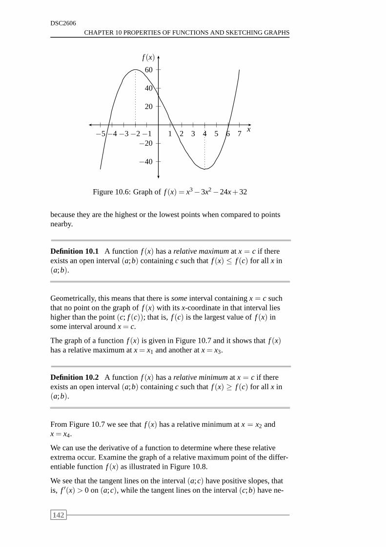
DSC2606
CHAPTER 10 PROPERTIES OF FUNCTIONS AND SKETCHING GRAPHS
20
40
60
−20
−40
1 2 3 4 5 6 7−1−2−3−4−5x
f (x)
Figure 10.6: Graph off (x) = x3−3x2−24x+32
because they are the highest or the lowest points when compared to pointsnearby.
Definition 10.1 A function f (x) has arelative maximumat x = c if thereexists an open interval(a;b) containingc such thatf (x) ≤ f (c) for all x in(a;b).
Geometrically, this means that there issomeinterval containingx = c suchthat no point on the graph off (x) with its x-coordinate in that interval lieshigher than the point(c; f (c)); that is, f (c) is the largest value off (x) insome interval aroundx= c.
The graph of a functionf (x) is given in Figure 10.7 and it shows thatf (x)has a relative maximum atx= x1 and another atx= x3.
Definition 10.2 A function f (x) has arelative minimumat x = c if thereexists an open interval(a;b) containingc such thatf (x) ≥ f (c) for all x in(a;b).
From Figure 10.7 we see thatf (x) has a relative minimum atx = x2 andx= x4.
We can use the derivative of a function to determine where these relativeextrema occur. Examine the graph of a relative maximum pointof the differ-entiable functionf (x) as illustrated in Figure 10.8.
We see that the tangent lines on the interval(a;c) have positive slopes, thatis, f ′(x)> 0 on(a;c), while the tangent lines on the interval(c;b) have ne-
142
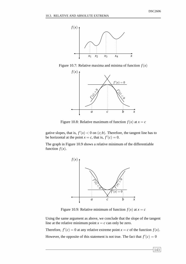
10.3. RELATIVE AND ABSOLUTE EXTREMA
DSC2606
x
f (x)
x1 x2 x3 x4
Figure 10.7: Relative maxima and minima of functionf (x)
x
f (x)
f′ (x)>
0 f ′(x)<0
f ′(x) = 0
ca b
Figure 10.8: Relative maximum of functionf (x) at x= c
gative slopes, that is,f ′(x)< 0 on(c;b). Therefore, the tangent line has tobe horizontal at the pointx= c, that is, f ′(c) = 0.
The graph in Figure 10.9 shows a relative minimum of the differentiablefunction f (x).
x
f (x)
f ′(x)<0 f
′ (x)>
0
f ′(x) = 0
ca b
Figure 10.9: Relative minimum of functionf (x) at x= c
Using the same argument as above, we conclude that the slope of the tangentline at the relative minimum pointx= c can only be zero.
Therefore,f ′(c) = 0 at any relative extreme pointx= c of the functionf (x).
However, the opposite of this statement is not true. The factthat f ′(c) = 0
143
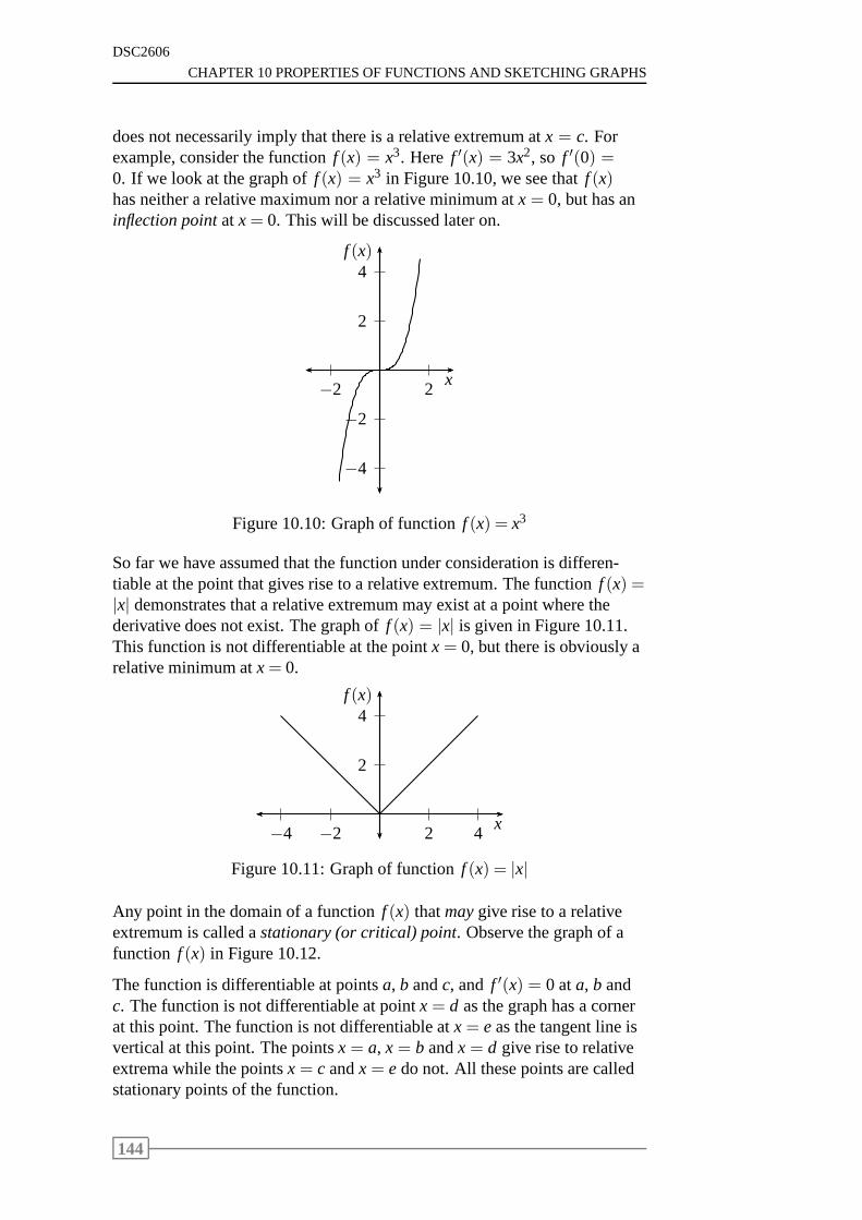
DSC2606
CHAPTER 10 PROPERTIES OF FUNCTIONS AND SKETCHING GRAPHS
does not necessarily imply that there is a relative extremumat x = c. Forexample, consider the functionf (x) = x3. Here f ′(x) = 3x2, so f ′(0) =0. If we look at the graph off (x) = x3 in Figure 10.10, we see thatf (x)has neither a relative maximum nor a relative minimum atx = 0, but has aninflection pointat x= 0. This will be discussed later on.
2
4
−2
−4
2−2x
f (x)
Figure 10.10: Graph of functionf (x) = x3
So far we have assumed that the function under considerationis differen-tiable at the point that gives rise to a relative extremum. The function f (x) =|x| demonstrates that a relative extremum may exist at a point where thederivative does not exist. The graph off (x) = |x| is given in Figure 10.11.This function is not differentiable at the pointx= 0, but there is obviously arelative minimum atx= 0.
2
4
2 4−2−4x
f (x)
Figure 10.11: Graph of functionf (x) = |x|
Any point in the domain of a functionf (x) thatmaygive rise to a relativeextremum is called astationary (or critical) point. Observe the graph of afunction f (x) in Figure 10.12.
The function is differentiable at pointsa, b andc, and f ′(x) = 0 ata, b andc. The function is not differentiable at pointx = d as the graph has a cornerat this point. The function is not differentiable atx= eas the tangent line isvertical at this point. The pointsx = a, x = b andx = d give rise to relativeextrema while the pointsx = c andx = e do not. All these points are calledstationary points of the function.
144
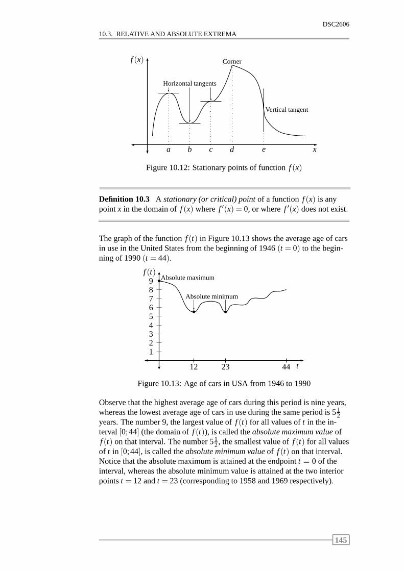
10.3. RELATIVE AND ABSOLUTE EXTREMA
DSC2606
x
f (x)
a b c d e
Horizontal tangents
Corner
Vertical tangent
Figure 10.12: Stationary points of functionf (x)
Definition 10.3 A stationary (or critical) pointof a function f (x) is anypointx in the domain off (x) where f ′(x) = 0, or wheref ′(x) does not exist.
The graph of the functionf (t) in Figure 10.13 shows the average age of carsin use in the United States from the beginning of 1946(t = 0) to the begin-ning of 1990(t = 44).
123456789
t
f (t)
12 23 44
b
b b
Absolute maximum
Absolute minimum
Figure 10.13: Age of cars in USA from 1946 to 1990
Observe that the highest average age of cars during this period is nine years,whereas the lowest average age of cars in use during the same period is 51
2years. The number 9, the largest value off (t) for all values oft in the in-terval[0;44] (the domain off (t)), is called theabsolute maximum valueoff (t) on that interval. The number 51
2, the smallest value off (t) for all valuesof t in [0;44], is called theabsolute minimum valueof f (t) on that interval.Notice that the absolute maximum is attained at the endpointt = 0 of theinterval, whereas the absolute minimum value is attained atthe two interiorpointst = 12 andt = 23 (corresponding to 1958 and 1969 respectively).
145

DSC2606
CHAPTER 10 PROPERTIES OF FUNCTIONS AND SKETCHING GRAPHS
Definition 10.4
• If f (x) < f (c) for all x in the domain off (x), then f (c) is called theabsolute maximum valueof f (x).
• If f (x) > f (c) for all x in the domain off (x), then f (c) is called theabsolute minimum valueof f (x).
A continuous function defined on an arbitrary interval does not always havean absolute maximum or an absolute minimum. However, an important caseoften arises in practical applications where both the absolute maximum andthe absolute minimum of a function are guaranteed to exist. This occurswhen a continuous function is defined on aclosedinterval.
Property 10.1 If a function f (x) is continuous on a closed interval[a;b],then f (x) has both an absolute maximum value and an absolute minimumvalue on[a;b].
The graph in Figure 10.14 illustrates a typical situation.
x
f (x)
b
b
b
b
b
a x1
Relativeminimum
x2 x3
Absoluteminimum
b
Absolutemaximum
Relativemaximum
Figure 10.14: Relative and absolute extrema of functionf (x) on [a;b]
Herex1, x2 andx3 are stationary points off (x). The absolute minimum off (x) occurs atx3. The absolute maximum off (x) occurs atb, an endpoint.
Example 10.3
Find the absolute extrema of the functionf (x) = x3− 2x2− 4x+ 4,defined on the interval[0;3].
146
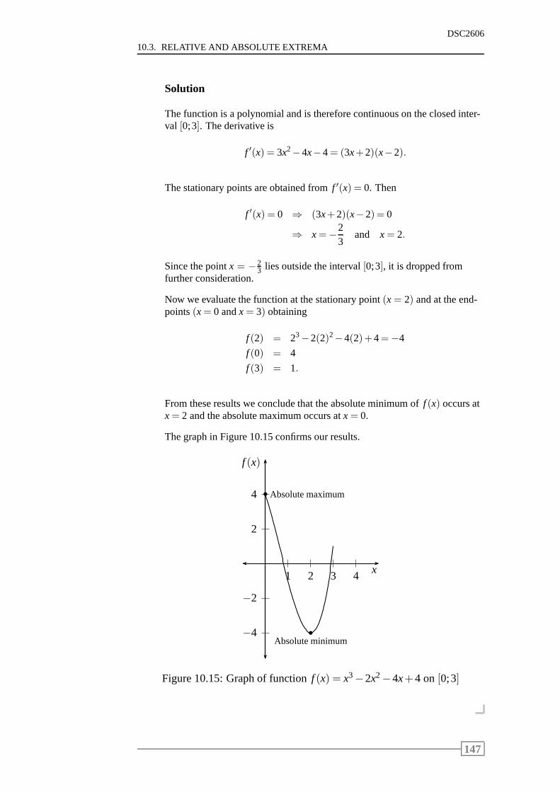
10.3. RELATIVE AND ABSOLUTE EXTREMA
DSC2606
Solution
The function is a polynomial and is therefore continuous on the closed inter-val [0;3]. The derivative is
f ′(x) = 3x2−4x−4= (3x+2)(x−2).
The stationary points are obtained fromf ′(x) = 0. Then
f ′(x) = 0 ⇒ (3x+2)(x−2)= 0
⇒ x=−23
and x= 2.
Since the pointx = −23 lies outside the interval[0;3], it is dropped from
further consideration.
Now we evaluate the function at the stationary point(x= 2) and at the end-points(x= 0 andx= 3) obtaining
f (2) = 23−2(2)2−4(2)+4=−4
f (0) = 4
f (3) = 1.
From these results we conclude that the absolute minimum off (x) occurs atx= 2 and the absolute maximum occurs atx= 0.
The graph in Figure 10.15 confirms our results.
2
4
−2
−4
1 2 3 4x
f (x)
b
b
Absolute minimum
Absolute maximum
Figure 10.15: Graph of functionf (x) = x3−2x2−4x+4 on [0;3]
147
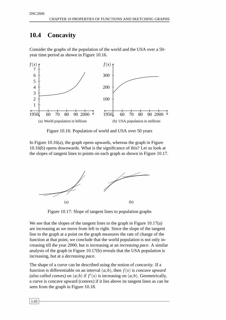
DSC2606
CHAPTER 10 PROPERTIES OF FUNCTIONS AND SKETCHING GRAPHS
10.4 Concavity
Consider the graphs of the population of the world and the USAover a 50-year time period as shown in Figure 10.16.
1234567
x
f (x)
1950 60 70 80 90 2000
(a) World population in billions
100
200
300
x
f (x)
1950 60 70 80 90 2000
(b) USA population in millions
Figure 10.16: Population of world and USA over 50 years
In Figure 10.16(a), the graph opens upwards, whereas the graph in Figure10.16(b) opens downwards. What is the significance of this? Let us look atthe slopes of tangent lines to points on each graph as shown inFigure 10.17.
(a) (b)
Figure 10.17: Slope of tangent lines to population graphs
We see that the slopes of the tangent lines to the graph in Figure 10.17(a)are increasing as we move from left to right. Since the slope of the tangentline to the graph at a point on the graph measures the rate of change of thefunction at that point, we conclude that the world population is not only in-creasing till the year 2000, but is increasing at anincreasing pace. A similaranalysis of the graph in Figure 10.17(b) reveals that the USApopulation isincreasing, but at adecreasing pace.
The shape of a curve can be described using the notion ofconcavity. If afunction is differentiable on an interval(a;b), then f (x) is concave upward(also called convex)on (a;b) if f ′(x) is increasing on(a;b). Geometrically,a curve is concave upward (convex) if it lies above its tangent lines as can beseen from the graph in Figure 10.18.
148
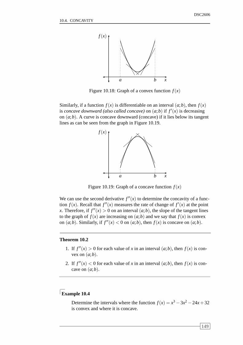
10.4. CONCAVITY
DSC2606
x
f (x)
a b
Figure 10.18: Graph of a convex functionf (x)
Similarly, if a function f (x) is differentiable on an interval(a;b), then f (x)is concave downward (also called concave)on (a;b) if f ′(x) is decreasingon (a;b). A curve is concave downward (concave) if it lies below its tangentlines as can be seen from the graph in Figure 10.19.
x
f (x)
a b
Figure 10.19: Graph of a concave functionf (x)
We can use the second derivativef ′′(x) to determine the concavity of a func-tion f (x). Recall thatf ′′(x) measures the rate of change off ′(x) at the pointx. Therefore, iff ′′(x) > 0 on an interval(a;b), the slope of the tangent linesto the graph off (x) are increasing on(a;b) and we say thatf (x) is convexon (a;b). Similarly, if f ′′(x)< 0 on(a;b), then f (x) is concave on(a;b).
Theorem 10.2
1. If f ′′(x) > 0 for each value ofx in an interval(a;b), then f (x) is con-vex on(a;b).
2. If f ′′(x) < 0 for each value ofx in an interval(a;b), then f (x) is con-cave on(a;b).
Example 10.4
Determine the intervals where the functionf (x) = x3−3x2−24x+32is convex and where it is concave.
149
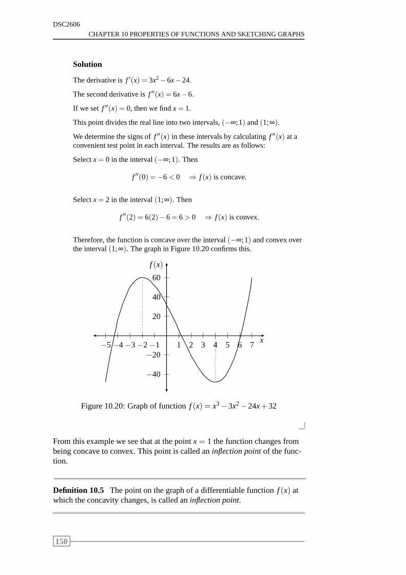
DSC2606
CHAPTER 10 PROPERTIES OF FUNCTIONS AND SKETCHING GRAPHS
Solution
The derivative isf ′(x) = 3x2−6x−24.
The second derivative isf ′′(x) = 6x−6.
If we set f ′′(x) = 0, then we findx= 1.
This point divides the real line into two intervals,(−∞;1) and(1;∞).
We determine the signs off ′′(x) in these intervals by calculatingf ′′(x) at aconvenient test point in each interval. The results are as follows:
Selectx= 0 in the interval(−∞;1). Then
f ′′(0) =−6< 0 ⇒ f (x) is concave.
Selectx= 2 in the interval(1;∞). Then
f ′′(2) = 6(2)−6= 6> 0 ⇒ f (x) is convex.
Therefore, the function is concave over the interval(−∞;1) and convex overthe interval(1;∞). The graph in Figure 10.20 confirms this.
20
40
60
−20
−40
1 2 3 4 5 6 7−1−2−3−4−5x
f (x)
Figure 10.20: Graph of functionf (x) = x3−3x2−24x+32
From this example we see that at the pointx= 1 the function changes frombeing concave to convex. This point is called aninflection pointof the func-tion.
Definition 10.5 The point on the graph of a differentiable functionf (x) atwhich the concavity changes, is called aninflection point.
150
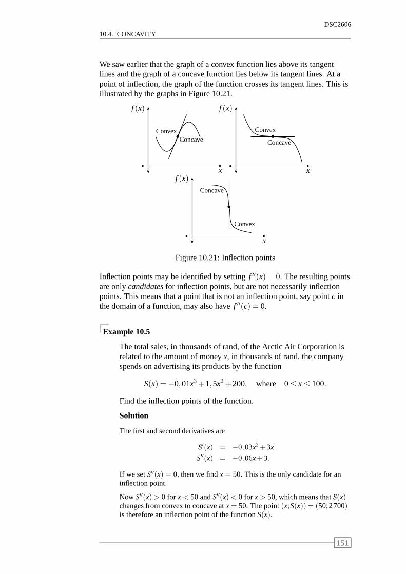
10.4. CONCAVITY
DSC2606
We saw earlier that the graph of a convex function lies above its tangentlines and the graph of a concave function lies below its tangent lines. At apoint of inflection, the graph of the function crosses its tangent lines. This isillustrated by the graphs in Figure 10.21.
x
f (x)
bConvex
Concave
x
f (x)
bConvex
Concave
x
f (x)
b
Concave
Convex
Figure 10.21: Inflection points
Inflection points may be identified by settingf ′′(x) = 0. The resulting pointsare onlycandidatesfor inflection points, but are not necessarily inflectionpoints. This means that a point that is not an inflection point, say pointc inthe domain of a function, may also havef ′′(c) = 0.
Example 10.5
The total sales, in thousands of rand, of the Arctic Air Corporation isrelated to the amount of moneyx, in thousands of rand, the companyspends on advertising its products by the function
S(x) =−0,01x3+1,5x2+200, where 0≤ x≤ 100.
Find the inflection points of the function.
Solution
The first and second derivatives are
S′(x) = −0,03x2+3x
S′′(x) = −0,06x+3.
If we setS′′(x) = 0, then we findx = 50. This is the only candidate for aninflection point.
Now S′′(x) > 0 for x< 50 andS′′(x) < 0 for x > 50, which means thatS(x)changes from convex to concave atx= 50. The point(x;S(x)) = (50;2700)is therefore an inflection point of the functionS(x).
151
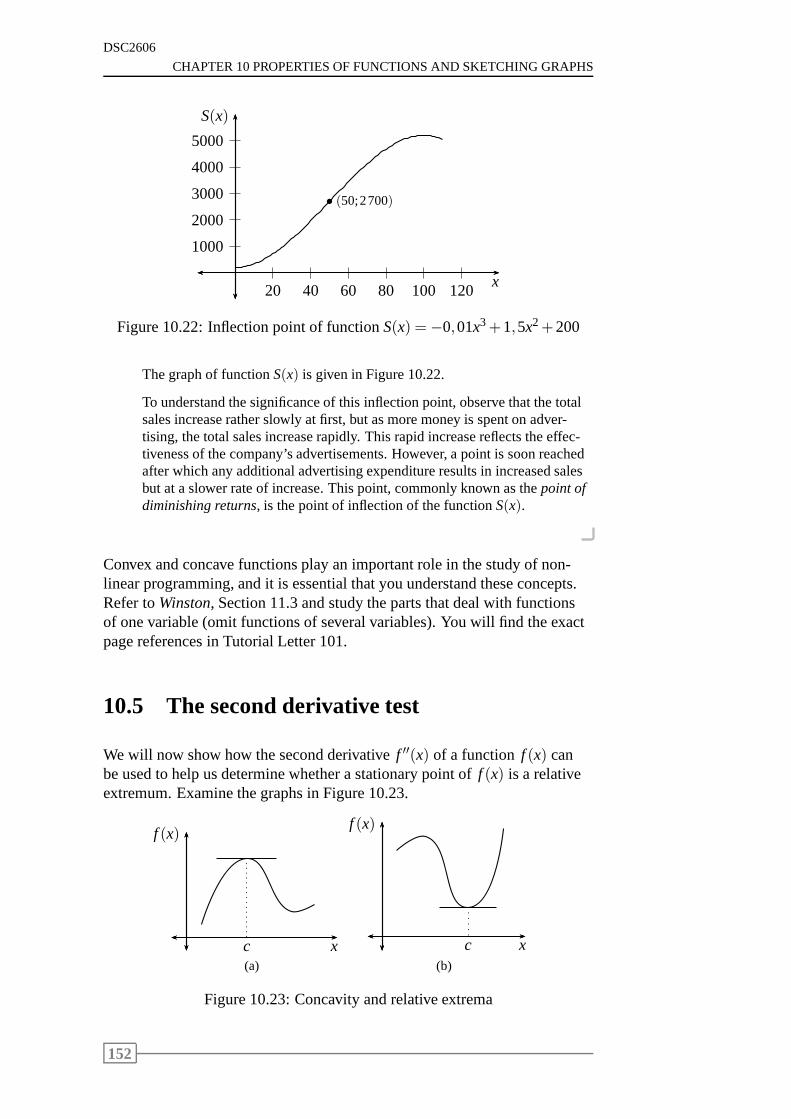
DSC2606
CHAPTER 10 PROPERTIES OF FUNCTIONS AND SKETCHING GRAPHS
1000
2000
3000
4000
5000
20 40 60 80 100 120x
S(x)
b (50;2700)
Figure 10.22: Inflection point of functionS(x) =−0,01x3+1,5x2+200
The graph of functionS(x) is given in Figure 10.22.
To understand the significance of this inflection point, observe that the totalsales increase rather slowly at first, but as more money is spent on adver-tising, the total sales increase rapidly. This rapid increase reflects the effec-tiveness of the company’s advertisements. However, a pointis soon reachedafter which any additional advertising expenditure results in increased salesbut at a slower rate of increase. This point, commonly known as thepoint ofdiminishing returns, is the point of inflection of the functionS(x).
Convex and concave functions play an important role in the study of non-linear programming, and it is essential that you understandthese concepts.Refer toWinston, Section 11.3 and study the parts that deal with functionsof one variable (omit functions of several variables). You will find the exactpage references in Tutorial Letter 101.
10.5 The second derivative test
We will now show how the second derivativef ′′(x) of a function f (x) canbe used to help us determine whether a stationary point off (x) is a relativeextremum. Examine the graphs in Figure 10.23.
x
f (x)
c(a)
x
f (x)
c(b)
Figure 10.23: Concavity and relative extrema
152
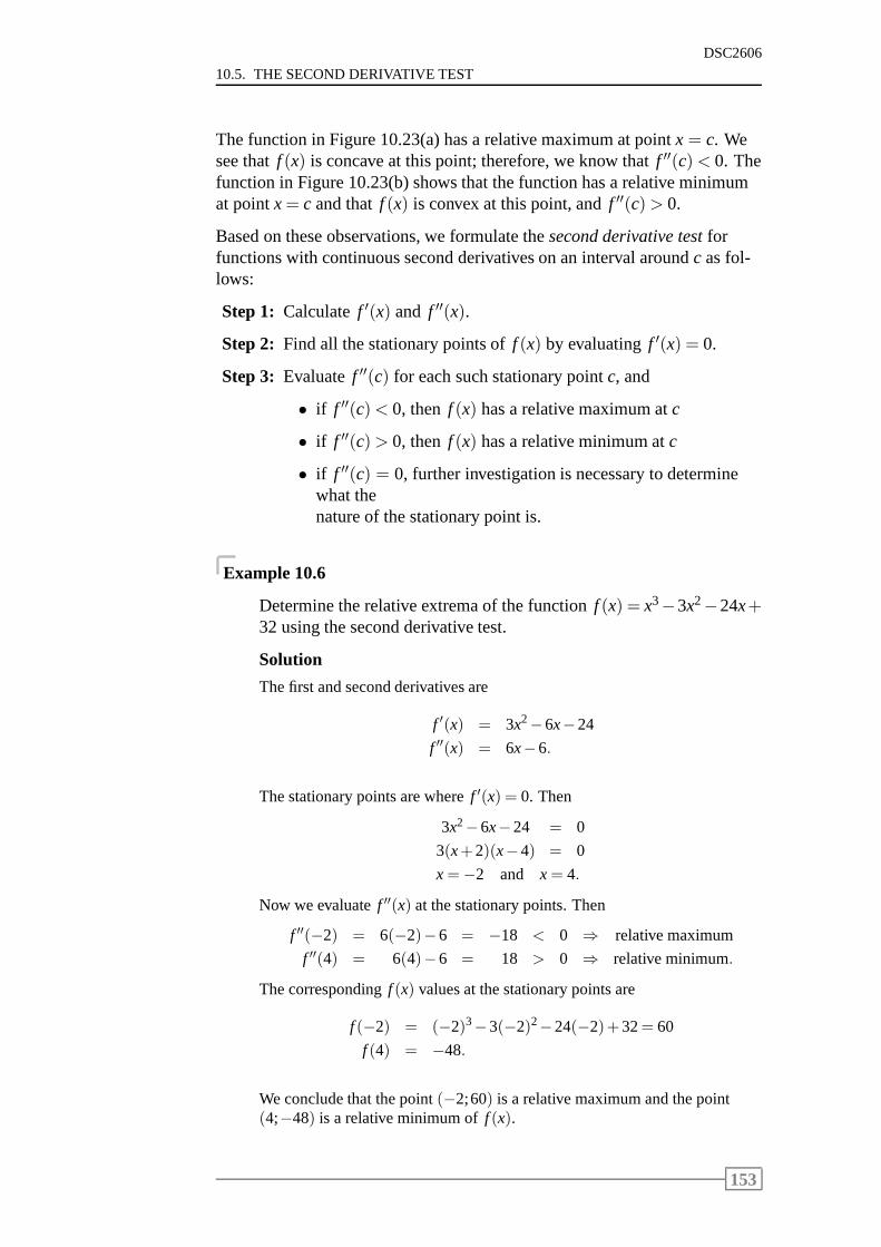
10.5. THE SECOND DERIVATIVE TEST
DSC2606
The function in Figure 10.23(a) has a relative maximum at point x = c. Wesee thatf (x) is concave at this point; therefore, we know thatf ′′(c)< 0. Thefunction in Figure 10.23(b) shows that the function has a relative minimumat pointx= c and thatf (x) is convex at this point, andf ′′(c)> 0.
Based on these observations, we formulate thesecond derivative testforfunctions with continuous second derivatives on an interval aroundc as fol-lows:
Step 1: Calculatef ′(x) and f ′′(x).
Step 2: Find all the stationary points off (x) by evaluatingf ′(x) = 0.
Step 3: Evaluatef ′′(c) for each such stationary pointc, and
• if f ′′(c)< 0, then f (x) has a relative maximum atc
• if f ′′(c)> 0, then f (x) has a relative minimum atc
• if f ′′(c) = 0, further investigation is necessary to determinewhat thenature of the stationary point is.
Example 10.6
Determine the relative extrema of the functionf (x) = x3−3x2−24x+32 using the second derivative test.
Solution
The first and second derivatives are
f ′(x) = 3x2−6x−24
f ′′(x) = 6x−6.
The stationary points are wheref ′(x) = 0. Then
3x2−6x−24 = 0
3(x+2)(x−4) = 0
x=−2 and x= 4.
Now we evaluatef ′′(x) at the stationary points. Then
f ′′(−2) = 6(−2)−6 = −18 < 0 ⇒ relative maximum
f ′′(4) = 6(4)−6 = 18 > 0 ⇒ relative minimum.
The correspondingf (x) values at the stationary points are
f (−2) = (−2)3−3(−2)2−24(−2)+32= 60
f (4) = −48.
We conclude that the point(−2;60) is a relative maximum and the point(4;−48) is a relative minimum off (x).
153
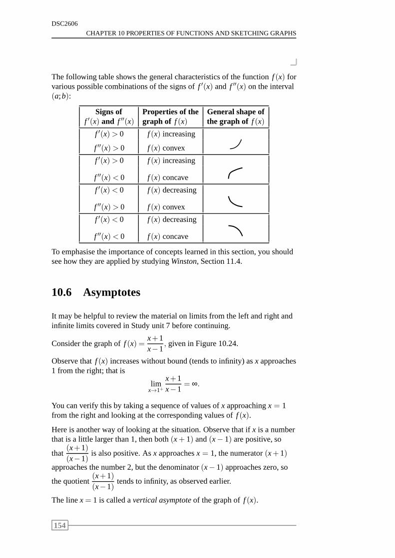
DSC2606
CHAPTER 10 PROPERTIES OF FUNCTIONS AND SKETCHING GRAPHS
The following table shows the general characteristics of the function f (x) forvarious possible combinations of the signs off ′(x) and f ′′(x) on the interval(a;b):
Signs of Properties of the General shape off ′(x) and f ′′(x) graph of f (x) the graph of f (x)
f ′(x)> 0 f (x) increasing
f ′′(x)> 0 f (x) convex
f ′(x)> 0 f (x) increasing
f ′′(x)< 0 f (x) concave
f ′(x)< 0 f (x) decreasing
f ′′(x)> 0 f (x) convex
f ′(x)< 0 f (x) decreasing
f ′′(x)< 0 f (x) concave
To emphasise the importance of concepts learned in this section, you shouldsee how they are applied by studyingWinston, Section 11.4.
10.6 Asymptotes
It may be helpful to review the material on limits from the left and right andinfinite limits covered in Study unit 7 before continuing.
Consider the graph off (x) =x+1x−1
, given in Figure 10.24.
Observe thatf (x) increases without bound (tends to infinity) asx approaches1 from the right; that is
limx→1+
x+1x−1
= ∞.
You can verify this by taking a sequence of values ofx approachingx = 1from the right and looking at the corresponding values off (x).
Here is another way of looking at the situation. Observe thatif x is a numberthat is a little larger than 1, then both(x+ 1) and(x− 1) are positive, so
that(x+1)(x−1)
is also positive. Asx approachesx = 1, the numerator(x+1)
approaches the number 2, but the denominator(x− 1) approaches zero, so
the quotient(x+1)(x−1)
tends to infinity, as observed earlier.
The linex= 1 is called avertical asymptoteof the graph off (x).
154
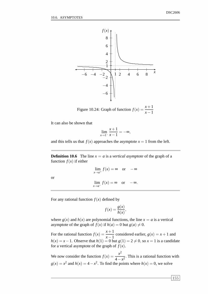
10.6. ASYMPTOTES
DSC2606
2
4
6
8
−2
−4
−6
2 4 6 8−2−4−6x
f (x)
1
1
Figure 10.24: Graph of functionf (x) =x+1x−1
It can also be shown that
limx→1−
x+1x−1
=−∞,
and this tells us thatf (x) approaches the asymptotex= 1 from the left.
Definition 10.6 The linex = a is avertical asymptoteof the graph of afunction f (x) if either
limx→a+
f (x) = ∞ or −∞
orlim
x→a−f (x) = ∞ or −∞.
For any rational functionf (x) defined by
f (x) =g(x)h(x)
,
whereg(x) andh(x) are polynomial functions, the linex = a is a verticalasymptote of the graph off (x) if h(a) = 0 butg(a) 6= 0.
For the rational functionf (x) =x+1x−1
considered earlier,g(x) = x+ 1 and
h(x) = x−1. Observe thath(1) = 0 butg(1) = 2 6= 0, sox= 1 is a candidatefor a vertical asymptote of the graph off (x).
We now consider the functionf (x) =x2
4−x2 . This is a rational function with
g(x) = x2 andh(x) = 4−x2. To find the points whereh(x) = 0, we solve
155
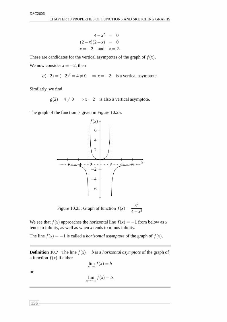
DSC2606
CHAPTER 10 PROPERTIES OF FUNCTIONS AND SKETCHING GRAPHS
4−x2 = 0
(2−x)(2+x) = 0
x=−2 and x= 2.
These are candidates for the vertical asymptotes of the graph of f (x).
We now considerx=−2, then
g(−2) = (−2)2 = 4 6= 0 ⇒ x=−2 is a vertical asymptote.
Similarly, we find
g(2) = 4 6= 0 ⇒ x= 2 is also a vertical asymptote.
The graph of the function is given in Figure 10.25.
2
4
6
−2
−4
−6
2 4 6−2−4−6x
f (x)
Figure 10.25: Graph of functionf (x) =x2
4−x2
We see thatf (x) approaches the horizontal linef (x) = −1 from below asxtends to infinity, as well as whenx tends to minus infinity.
The line f (x) =−1 is called ahorizontal asymptoteof the graph off (x).
Definition 10.7 The line f (x) = b is ahorizontal asymptoteof the graph ofa function f (x) if either
limx→∞
f (x) = b
orlim
x→−∞f (x) = b.
156
10.7. SKETCHING GRAPHS
DSC2606
For the functionf (x) =x+1x−1
we see that
limx→∞
x+1x−1
= limx→∞
1+ 1x
1− 1x
= 1,
if we divide the numerator and the denominator byx. Also,
limx→−∞
x+1x−1
= limx→−∞
1+ 1x
1− 1x
= 1.
In either case, we conclude thatf (x) = 1 is a horizontal asymptote of thegraph of f (x) as observed earlier.
Example 10.7
Calculate the horizontal asymptotes of the graph of the function f (x) =x2
4−x2 .
Solution
We calculate
limx→∞
x2
4−x2 = limx→∞
14x2 −1
=−1.
Therefore,f (x) =−1 is a horizontal asymptote.
NOTE:A polynomial function has no asymptotes.
10.7 Sketching graphs
We have now seen how the first and second derivatives of a function are usedto reveal various properties of the graph of the function. Wewill now showhow this information can be used to help us sketch the graph ofthe function.We begin by giving a general procedure for sketching graphs of functionsf (x) as follows:
Step 1: Determine the domain off (x).
Step 2: Find the intercepts off (x) on the axes. The equationf (x) = 0 maybe difficult to solve, in which case one may need to search for thex-intercepts numerically. Numerical search algorithms such as thebisection method and Newton’s method are discussed in the nextstudy unit.
Step 3: Determine the behaviour off (x) for large absolute values ofx.
157
DSC2606
CHAPTER 10 PROPERTIES OF FUNCTIONS AND SKETCHING GRAPHS
Step 4: Find all horizontal and vertical asymptotes off (x).
Step 5: Determine the intervals wheref (x) is increasing and where it isdecreasing.
Step 6: Find the relative extrema off (x).
Step 7: Determine the concavity off (x) and find the inflection points off (x).
Step 8: Plot a few additional points to help further identify the shape of thegraph of f (x), and sketch the graph.
Example 10.8
Sketch the graph of the functiony= f (x) =x+1x−1
.
Solution
Step 1: The function is not defined forx = 1 since division by zero is notallowed. The domain off (x) is the set of all real numbers otherthanx= 1.
Step 2: They-intercept is found by settingx= 0. Then
y= f (0) =−1.
Thex-intercept is found by settingy= f (x) = 0. Then
x+1x−1
= 0
x+1 = 0
x = −1.
Step 3: The behaviour off (x) for large absolute values ofx. We saw ear-lier that
limx→∞
x+1x−1
= 1
limx→−∞
x+1x−1
= 1.
Therefore,f (x) approaches the liney= 1 as|x| becomes large.
Step 4: From the results of step 3, we conclude thaty = 1 is a horizontalasymptote.
We saw earlier that
limx→1+
x+1x−1
= ∞
limx→1−
x+1x−1
= −∞.
Therefore,x= 1 is a vertical asymptote.
158

10.7. SKETCHING GRAPHS
DSC2606
Step 5: The derivative is
f ′(x) = (x+1)ddx
(x−1)−1+(x−1)−1 ddx
(x+1)
= (x+1)(−1)(x−1)−2+(x−1)−1(1)
=−(x+1)(x−1)2 +
1x−1
=−x−1+x−1
(x−1)2
=−2
(x−1)2 .
On the interval(−∞;1): f ′(x)< 0 ⇒ f (x) is decreasing.On the interval(1;∞): f ′(x)< 0 ⇒ f (x) is decreasing.
Step 6: We see thatf ′(x) 6= 0 for all values ofx in the intervals(−∞;1)and(1;∞). This means thatf (x) has no stationary points.
Step 7: The second derivative is
f ′′(x) =ddx
[
−2(x−1)−2]
= −2(−2)(x−1)−3
=4
(x−1)3 .
On the interval(−∞;1): f ′′(x)< 0 ⇒ f (x) is concave.On the interval(1;∞): f ′′(x)> 0 ⇒ f (x) is convex.
We see thatf ′′(x) 6= 0 for all values ofx in the intervals(−∞;1)and(1;∞). This means that there are no inflection points.
Step 8: Points onf (x) are as follows:
x −5 −4 −3 −2 0,5 1,5 2 3 4 5
f (x) 0,667 0,6 0,5 0,333 −3 5 3 2 1,667 1,5
The graph off (x) is given in Figure 10.26.
159
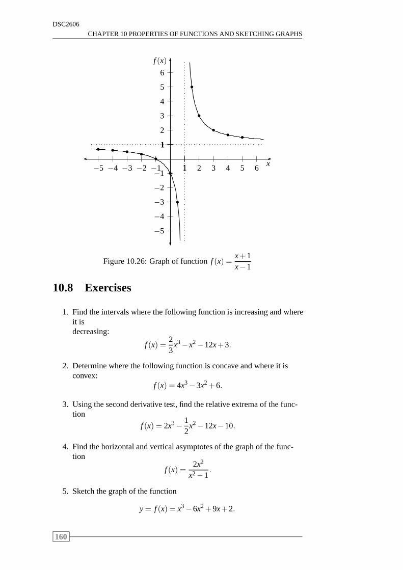
DSC2606
CHAPTER 10 PROPERTIES OF FUNCTIONS AND SKETCHING GRAPHS
1
2
3
4
5
6
−1
−2
−3
−4
−5
1 2 3 4 5 6−1−2−3−4−5x
f (x)
1
1b b b bb
b
b
b
b
bb b
Figure 10.26: Graph of functionf (x) =x+1x−1
10.8 Exercises
1. Find the intervals where the following function is increasing and whereit isdecreasing:
f (x) =23
x3−x2−12x+3.
2. Determine where the following function is concave and where it isconvex:
f (x) = 4x3−3x2+6.
3. Using the second derivative test, find the relative extrema of the func-tion
f (x) = 2x3− 12
x2−12x−10.
4. Find the horizontal and vertical asymptotes of the graph of the func-tion
f (x) =2x2
x2−1.
5. Sketch the graph of the function
y= f (x) = x3−6x2+9x+2.
160
10.9. SOLUTIONS TO EXERCISES
DSC2606
10.9 Solutions to exercises
1. The derivative isf ′(x) = 2x2−2x−12.
If we set f ′(x) = 0, we have
2x2−2x−12 = 0
x2−x−6 = 0
(x+2)(x−3) = 0
x=−2 and x= 3.
These points divide the real line into the intervals(−∞;−2), (−2;3)and(3;∞).
To determine the signs off ′(x) in these intervals, we calculatef ′(x) ata convenient test point in each interval. The results are as follows:
Selectx=−3 in the interval(−∞;−2). Then
f ′(−3) = 2(−3)2−2(−3)−12= 12> 0 ⇒ f (x) is increasing.
Selectx= 0 in the interval(−2;3). Then
f ′(0) =−12< 0 ⇒ f (x) is decreasing.
Selectx= 4 in the interval(3;∞). Then
f ′(4) = 12> 0 ⇒ f (x) is increasing.
Therefore,f (x) is increasing over(−∞;−2) and(3;∞), and it is de-creasing over(−2;3).
2. The first and second derivatives are
f ′(x) = 12x2−6x
f ′′(x) = 24x−6.
If we set f ′′(x) = 0, we have
24x−6 = 0
x =14.
This point divides the real line into two intervals(−∞; 14) and(1
4;∞).
Selectx= 0 in the interval(−∞; 14). Then
f ′′(0) = 24(0)−6=−6< 0 ⇒ f (x) is concave.
161
DSC2606
CHAPTER 10 PROPERTIES OF FUNCTIONS AND SKETCHING GRAPHS
Selectx= 1 in the interval(14;∞). Then
f ′′(1) = 24(1)−6= 18> 0 ⇒ f (x) is convex.
Therefore,f (x) is concave over(−∞; 14), and it is convex over(1
4;∞).
3. The first and second derivatives are
f ′(x) = 6x2−x−12
f ′′(x) = 12x−1.
The stationary points are obtained fromf ′(x) = 0. Then
6x2−x−12 = 0
(3x+4)(2x−3) = 0
x=−43 and x= 3
2
x=−1,333 and x= 1,5.
Now for x=−1,333 we have
f ′′(−1,333) = 12(−1,333)−1=−17< 0 ⇒ relative maximum.
The corresponding value off (x) at x=−1,333 is
f (−1,333)= 2(−1,333)3−0,5(−1,333)2−12(−1,333)−10= 0,37.
Therefore, point(−1,333;0,37) is a relative maximum.
Now for x= 1,5 we have
f ′′(1,5) = 12(1,5)−1= 17> 0 ⇒ relative minimum.
The corresponding value off (x) at x= 1,5 is
f (1,5) = 2(1,5)3−0,5(1,5)2−12(1,5)−10=−22,375.
Therefore, point(1,5;−22,375) is a relative minimum.
4. Letg(x) = 2x2 andh(x) = x2− 1, then f (x) =2x2
x2−1is a rational
function.
To find the points whereh(x) = 0, we solve
x2−1 = 0
x= 1 and x=−1.
162
10.9. SOLUTIONS TO EXERCISES
DSC2606
These are candidates for the vertical asymptotes.
We considerx= 1. Then
g(1) = 2(1)2 = 2 6= 0 ⇒ x= 1 is a vertical asymptote.
If we considerx= −1, theng(−1) = 2 6= 0, which means thatx= −1is also a vertical asymptote.
We can write
limx→∞
2x2
x2−1= lim
x→∞
2
1− 1x2
= 2.
This means thatf (x) = 2 is a horizontal asymptote.
Therefore, the graph of the function has vertical asymptotes atx= ±1and a horizontal asymptote atf (x) = 2.
5. The following information is obtained:
Step 1: The domain off (x) is the interval(−∞;∞).
Step 2: They-intercept is found by settingx= 0 and this is aty= 2.
Thex-intercept is found by settingy = f (x) = 0. In thiscase, it is a cubic equation. The solution to this equation canbe found by applying a numerical search procedure. This isdiscussed in the next study unit.
Step 3: Since
limx→−∞
f (x) = limx→−∞
(x3−6x2+9x+2) =−∞,
andlimx→∞
f (x) = limx→∞
(x3−6x2+9x+2) = ∞,
we see thatf (x) decreases without bound asx tends to mi-nus infinity, andf (x) increases without bound asx tends toinfinity.
Step 4: Since f (x) is a polynomial, there are no asymptotes.
Step 5: The first derivative isf ′(x) = 3x2−12x+9. If we set f ′(x) =0, we have
3x2−12x+9 = 0
3(x2−4x+3) = 0
3(x−1)(x−3) = 0
x= 1 and x= 3.
These points divide the line into the intervals(−∞;1), (1;3)and(3;∞).
163
DSC2606
CHAPTER 10 PROPERTIES OF FUNCTIONS AND SKETCHING GRAPHS
Selectx= 0 in the interval(−∞;1). Then
f ′(0) = 9> 0 ⇒ f (x) is increasing.
Selectx= 2 in the interval(1;3). Then
f ′(2) = 3(2)2−12(2)+9=−3< 0 ⇒ f (x) is decreasing.
Selectx= 4 in the interval(3;∞). Then
f ′(4) = 3(4)2−12(4)+9= 9> 0 ⇒ f (x) is increasing.
Step 6: The second derivative isf ′′(x) = 6x−12.
The stationary points,x= 1 andx= 3, were found by settingf ′(x) = 0 in Step 5 above. Evaluating the second derivativeat the stationary points gives
f ′′(1) = 6(1)−12 = −6 < 0 ⇒ relative maximum
f ′′(3) = 6(3)−12 = 6 > 0 ⇒ relative minimum.
The correspondingf (x) values are
f (1) = 13−6(1)2+9(1)+2 = 6
f (3) = 33−6(3)2+9(3)+2 = 2.
The point(1;6) is a relative maximum and the point(3;2) isa relative minimum.
Step 7: If we set f ′′(x) = 0, then we have 6x−12= 0 ⇒ x= 2.
This point is a candidate for an inflection point and it dividesthe real line into two intervals(−∞;2) and(2;∞).
Selectx= 0 in the interval(−∞;2). Then
f ′′(0) = 6(0)−12=−12< 0 ⇒ f (x) is concave.
Selectx= 3 in the interval(2;∞). Then
f ′′(3) = 6(3)−12= 6> 0 ⇒ f (x) is convex.
We see thatf (x) changes from a concave to a convex func-tion atx = 2; therefore, it is an inflection point. The corre-spondingf (x) value is
f (2) = 23−6(2)2+9(2)+2= 4.
Point(2;4) is an inflection point.
164
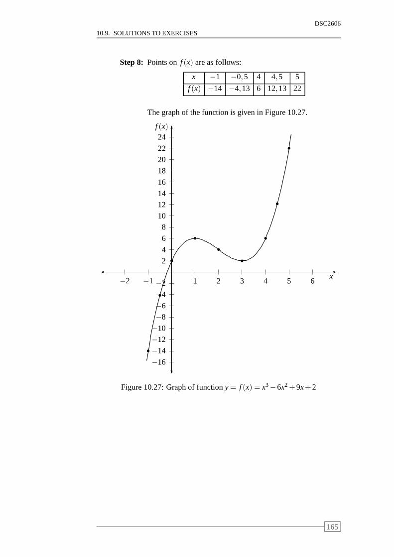
10.9. SOLUTIONS TO EXERCISES
DSC2606
Step 8: Points onf (x) are as follows:
x −1 −0,5 4 4,5 5
f (x) −14 −4,13 6 12,13 22
The graph of the function is given in Figure 10.27.
2
4
6
8
10
12
14
16
18
20
22
24
−2
−4
−6
−8
−10
−12
−14
−16
1 2 3 4 5 6−1−2x
f (x)
b
b
b
b
b
b
b
b
b
Figure 10.27: Graph of functiony= f (x) = x3−6x2+9x+2
165

DSC2606
CHAPTER 10 PROPERTIES OF FUNCTIONS AND SKETCHING GRAPHS
166

Chapter 11
Zeros of functions or roots ofequations
Contents11.1 Introduction . . . . . . . . . . . . . . . . . . . . . . . . 168
11.2 Locating roots of equations . . . . . . . . . . . . . . . . 168
11.3 Bisection method . . . . . . . . . . . . . . . . . . . . . . 170
11.3.1 Computer algorithms . . . . . . . . . . . . . . . . 173
11.4 Newton’s method . . . . . . . . . . . . . . . . . . . . . . 176
11.4.1 Computer algorithms . . . . . . . . . . . . . . . . 179
11.5 Exercises . . . . . . . . . . . . . . . . . . . . . . . . . . 182
11.6 Solutions to exercises . . . . . . . . . . . . . . . . . . . 183
167
DSC2606
CHAPTER 11 ZEROS OF FUNCTIONS OR ROOTS OF EQUATIONS
Learning objectivesAfter completing this study unit you should be able to
• determine zeros of functions or roots of equations algebraically, wherepossible, or else numerically
• apply numerical search algorithms, such as the bisection method andNewton’s method, to approximate zeros of functions or rootsof equa-tions
• implement iterative procedures of numerical search algorithms to ap-proximate zeros of functions or roots of equations in a computer pack-age such as Maxima
11.1 Introduction
When we sketched the graphs of functions in the previous study unit, it wassometimes difficult to determine thex-intercepts algebraically. We men-tioned that we might need to search for them numerically.
In this study unit we discuss two numerical search algorithms for determin-ing thex-intercepts, namely the bisection method and Newton’s method. Wealso discuss how to implement the iterative procedures of these two algo-rithms in Maxima.
If you have not done so yet, you should now install Maxima on your com-puter and work through the Maxima Programming Tutorial in Tutorial Let-ter 101.
11.2 Locating roots of equations
The notes in this study unit have been developed by referringto the text-booksNumerical Mathematics and Computingby Ward Cheney and DavidKincaid, andNumerical methods for Mathematics, Science and Engineeringby John H Mathews.
Definition 11.1 Assumef (x) is a continuous function. Any real numberrfor which f (r) = 0, is called theroot of the equation f(x) = 0 or thezero ofthe function f.
168
11.2. LOCATING ROOTS OF EQUATIONS
DSC2606
The zeros of the quadratic functionf (x) = ax2+bx+ c or the roots of theequationax2+bx+c= 0 can be easily calculated with the formula
x=−b±
√b2−4ac
2a.
Example 11.1
The equation 6x2−7x+2 = 0 has two real rootsr1 = 12 andr2 =
23.
Hence the functionf (x) = 6x2−7x+2 has12 and2
3 as zeros.
The zeros could be calculated using factorising
6x2−7x+2= (2x−1)(3x−2) = 0,
which means that either 2x−1 = 0 or 3x−2 = 0, or by applying theformula
r i =−(−7)±
√
(−7)2−4(6)(2)2(6)
.
In the case of a quadratic equation or parabola or polynomialof degree 2, wecan calculate the roots without any trouble. However, how doyou determinethe solution(s) of equations such as
0,5x5−7,32x4+31,344x3−18,464x2−79,104x−32,256= 0,
3560= 1000(1+ i)5−1
i(1+ i)5
or2x(1−x2+x) lnx= x2−1?
All the previous equations can be written in the formf (x) = 0. But it isimpossible to solve them algebraically. We need computer based methodsbased on iterative procedures (sometimes called trail-and-error methods) todetermine the solutions.
Quite a number of methods are available for locating the zeros of a nonlinearfunction. In this study unit we discuss two methods (the bisection methodand Newton’s method) to explain iterative procedures to approximate zeros.
We also explain how these methods can be implemented using Maxima.However, you may implement the algorithms using any other computer lan-guage (such as Java, C, Visual Basic) of your choice . The methods couldalso be implemented on any programmable pocket calculator.Maxima can-not be considered the most suitable package for numerical algorithms, butthe package is also used in other modules offered by the Department of De-cision Sciences, and can be used interactively to simplify numerical calcula-tions.
169
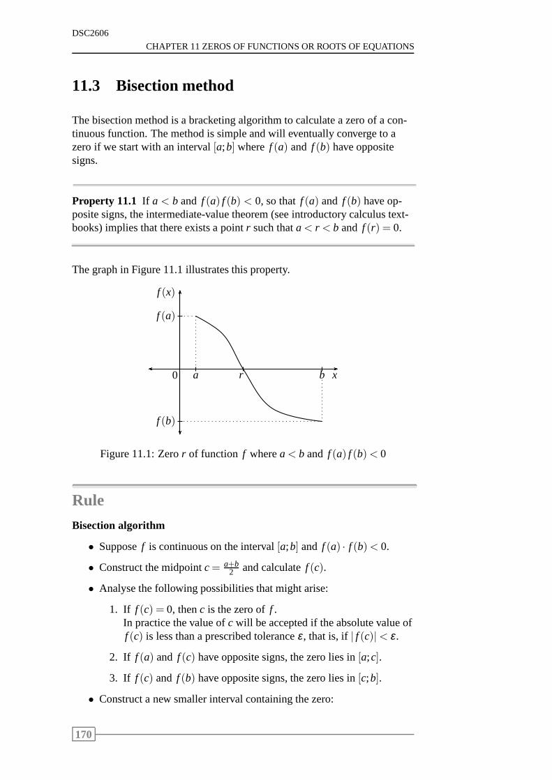
DSC2606
CHAPTER 11 ZEROS OF FUNCTIONS OR ROOTS OF EQUATIONS
11.3 Bisection method
The bisection method is a bracketing algorithm to calculatea zero of a con-tinuous function. The method is simple and will eventually converge to azero if we start with an interval[a;b] where f (a) and f (b) have oppositesigns.
Property 11.1 If a < b and f (a) f (b) < 0, so thatf (a) and f (b) have op-posite signs, the intermediate-value theorem (see introductory calculus text-books) implies that there exists a pointr such thata< r < b and f (r) = 0.
The graph in Figure 11.1 illustrates this property.
x
f (x)
f (a)
a
f (b)
b0 r
Figure 11.1: Zeror of function f wherea< b and f (a) f (b)< 0
Rule
Bisection algorithm
• Supposef is continuous on the interval[a;b] and f (a) · f (b)< 0.
• Construct the midpointc= a+b2 and calculatef (c).
• Analyse the following possibilities that might arise:
1. If f (c) = 0, thenc is the zero off .In practice the value ofc will be accepted if the absolute value off (c) is less than a prescribed toleranceε, that is, if| f (c)|< ε.
2. If f (a) and f (c) have opposite signs, the zero lies in[a;c].
3. If f (c) and f (b) have opposite signs, the zero lies in[c;b].
• Construct a new smaller interval containing the zero:
170
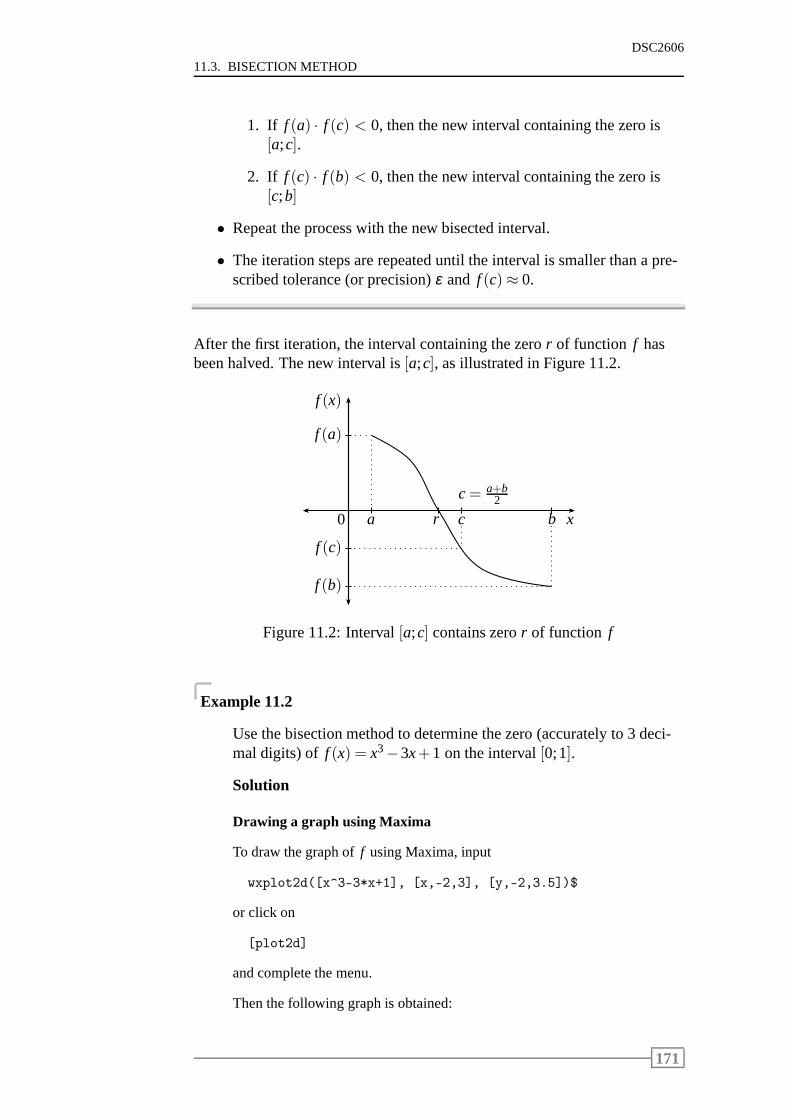
11.3. BISECTION METHOD
DSC2606
1. If f (a) · f (c) < 0, then the new interval containing the zero is[a;c].
2. If f (c) · f (b) < 0, then the new interval containing the zero is[c;b]
• Repeat the process with the new bisected interval.
• The iteration steps are repeated until the interval is smaller than a pre-scribed tolerance (or precision)ε and f (c)≈ 0.
After the first iteration, the interval containing the zeror of function f hasbeen halved. The new interval is[a;c], as illustrated in Figure 11.2.
x
f (x)
f (a)
a
f (b)
b0 r c
c= a+b2
f (c)
Figure 11.2: Interval[a;c] contains zeror of function f
Example 11.2
Use the bisection method to determine the zero (accurately to 3 deci-mal digits) of f (x) = x3−3x+1 on the interval[0;1].
Solution
Drawing a graph using Maxima
To draw the graph off using Maxima, input
wxplot2d([x^3-3*x+1], [x,-2,3], [y,-2,3.5])$
or click on
[plot2d]
and complete the menu.
Then the following graph is obtained:
171
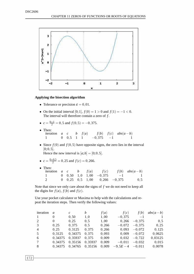
DSC2606
CHAPTER 11 ZEROS OF FUNCTIONS OR ROOTS OF EQUATIONS
Applying the bisection algorithm
• Tolerance or precisionε = 0,01.
• On the initial interval[0;1], f (0) = 1> 0 and f (1) =−1< 0.The interval will therefore contain a zero off .
• c= 0+12 = 0,5 and f (0,5) =−0,375.
• Then:iteration a c b f(a) f (b) f (c) abs(a−b)1 0 0,5 1 1 −0,375 −1 1
• Since f (0) and f (0,5) have opposite signs, the zero lies in the interval[0;0,5].Hence the new interval is[a;b] = [0;0,5].
• c= 0+0,52 = 0,25 andf (c) = 0,266.
• Then:iteration a c b f(a) f (c) f (b) abs(a−b)1 0 0,50 1,0 1,00 −0,375 −1 12 0 0,25 0,5 1,00 0,266 −0,375 0,5
Note that since we only care about the signs off we do not need to keep allthe digits for f (a), f (b) and f (c).
Use your pocket calculator or Maxima to help with the calculations and re-peat the iteration steps. Then verify the following values:
iteration a c b f(a) f (c) f (b) abs(a−b)1 0 0,50 1,0 1,00 −0,375 −1 12 0 0,25 0,5 1,00 0,266 −0,375 0,53 0,25 0,375 0,5 0,266 −0,072 −0,375 0,254 0,25 0,3125 0,375 0,266 0,093 −0,072 0,1255 0,3125 0,34375 0,375 0,093 0,009 −0,072 0,06256 0,34375 0,35937 0,375 0,009 0,032 −0,722 0,031257 0,34375 0,35156 0,35937 0,009 −0,011 −0,032 0,0158 0,34375 0,34765 0,35156 0,009 −9,5E−4 −0,011 0,0078
172
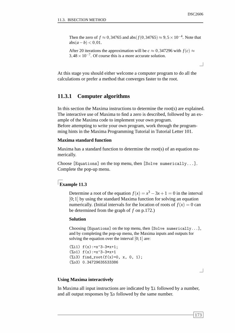
11.3. BISECTION METHOD
DSC2606
Then the zero off ≈ 0,34765 and abs( f (0,34765)≈ 9,5×10⁻⁴. Note thatabs(a−b)< 0,01.
After 20 iterations the approximation will bec ≈ 0,347296 withf (c) ≈3,48×10⁻⁷. Of course this is a more accurate solution.
At this stage you should either welcome a computer program todo all thecalculations or prefer a method that converges faster to theroot.
11.3.1 Computer algorithms
In this section the Maxima instructions to determine the root(s) are explained.The interactive use of Maxima to find a zero is described, followed by an ex-ample of the Maxima code to implement your own program.Before attempting to write your own program, work through the program-ming hints in the Maxima Programming Tutorial in Tutorial Letter 101.
Maxima standard function
Maxima has a standard function to determine the root(s) of anequation nu-merically.
Choose[Equations] on the top menu, then[Solve numerically...].Complete the pop-up menu.
Example 11.3
Determine a root of the equationf (x) = x3−3x+1= 0 in the interval[0;1] by using the standard Maxima function for solving an equationnumerically. (Initial intervals for the location of roots of f (x) = 0 canbe determined from the graph off on p.172.)
Solution
Choosing[Equations] on the top menu, then[Solve numerically...],and by completing the pop-up menu, the Maxima inputs and outputs forsolving the equation over the interval[0;1] are:
(%i1) f(x):=x^3-3*x+1;
(%o1) f(x):=x^3-3*x+1
(%i3) find_root(f(x)=0, x, 0, 1);
(%o3) 0.34729635533386
Using Maxima interactively
In Maxima all input instructions are indicated by%i followed by a number,and all output responses by%o followed by the same number.
173
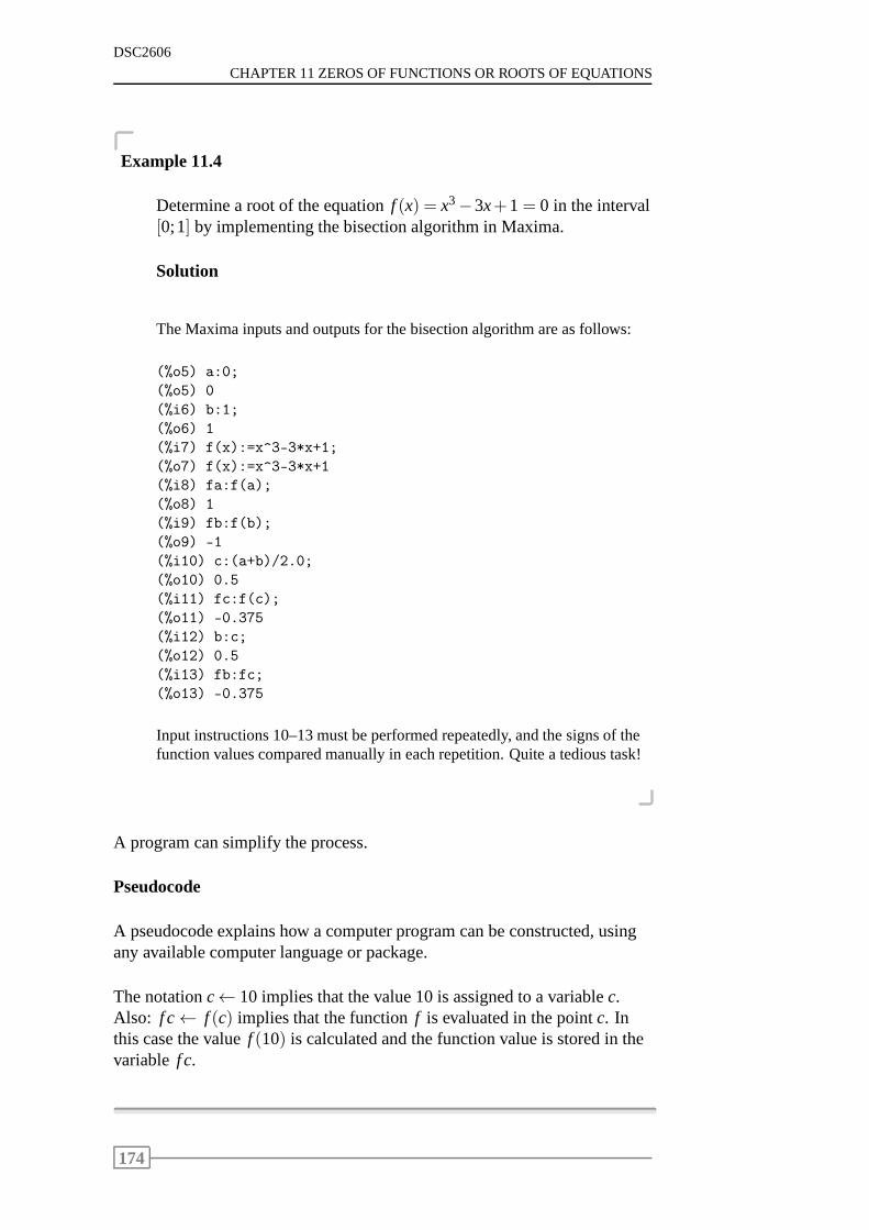
DSC2606
CHAPTER 11 ZEROS OF FUNCTIONS OR ROOTS OF EQUATIONS
Example 11.4
Determine a root of the equationf (x) = x3−3x+1= 0 in the interval[0;1] by implementing the bisection algorithm in Maxima.
Solution
The Maxima inputs and outputs for the bisection algorithm are as follows:
(%o5) a:0;
(%o5) 0
(%i6) b:1;
(%o6) 1
(%i7) f(x):=x^3-3*x+1;
(%o7) f(x):=x^3-3*x+1
(%i8) fa:f(a);
(%o8) 1
(%i9) fb:f(b);
(%o9) -1
(%i10) c:(a+b)/2.0;
(%o10) 0.5
(%i11) fc:f(c);
(%o11) -0.375
(%i12) b:c;
(%o12) 0.5
(%i13) fb:fc;
(%o13) -0.375
Input instructions 10–13 must be performed repeatedly, andthe signs of thefunction values compared manually in each repetition. Quite a tedious task!
A program can simplify the process.
Pseudocode
A pseudocode explains how a computer program can be constructed, usingany available computer language or package.
The notationc← 10 implies that the value 10 is assigned to a variablec.Also: f c← f (c) implies that the functionf is evaluated in the pointc. Inthis case the valuef (10) is calculated and the function value is stored in thevariable f c.
174
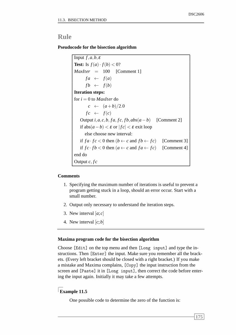
11.3. BISECTION METHOD
DSC2606
RulePseudocode for the bisection algorithm
Input f ,a,b,εTest: Is f (a) · f (b)< 0?
MaxIter = 100 [Comment 1]
f a ← f (a)
f b ← f (b)
Iteration steps:
for i = 0 to MaxIter do
c ← (a+b)/2.0
f c ← f (c)
Outputi,a,c,b, f a, f c, f b,abs(a−b) [Comment 2]
if abs(a−b)< ε or | f c|< ε exit loop
else choose new interval:
if f a · f c< 0 then(b← c and f b← f c) [Comment 3]
if f c· f b< 0 then(a← c and f a← f c) [Comment 4]
end do
Outputc, f c
Comments
1. Specifying the maximum number of iterations is useful to prevent aprogram getting stuck in a loop, should an error occur. Startwith asmall number.
2. Output only necessary to understand the iteration steps.
3. New interval[a;c]
4. New interval[c;b]
Maxima program code for the bisection algorithm
Choose[Edit] on the top menu and then[Long input] and type the in-structions. Then[Enter] the input. Make sure you remember all the brack-ets. (Every left bracket should be closed with a right bracket.) If you makea mistake and Maxima complains,[Copy] the input instruction from thescreen and[Paste] it in [Long input], then correct the code before enter-ing the input again. Initially it may take a few attempts.
Example 11.5
One possible code to determine the zero of the function is:
175
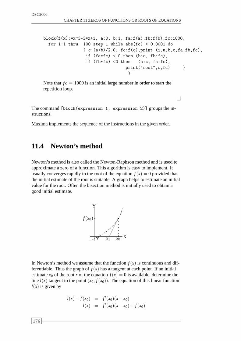
DSC2606
CHAPTER 11 ZEROS OF FUNCTIONS OR ROOTS OF EQUATIONS
block(f(x):=x^3-3*x+1, a:0, b:1, fa:f(a),fb:f(b),fc:1000,
for i:1 thru 100 step 1 while abs(fc) > 0.0001 do
( c:(a+b)/2.0, fc:f(c),print (i,a,b,c,fa,fb,fc),
if (fa*fc) < 0 then (b:c, fb:fc),
if (fb*fc) <0 then (a:c, fa:fc),
print("root",c,fc) )
)
Note thatf c = 1000 is an initial large number in order to start therepetition loop.
The command[block(expression 1, expression 2)] groups the in-structions.
Maxima implements the sequence of the instructions in the given order.
11.4 Newton’s method
Newton’s method is also called the Newton-Raphson method and is used toapproximate a zero of a function. This algorithm is easy to implement. Itusually converges rapidly to the root of the equationf (x) = 0 provided thatthe initial estimate of the root is suitable. A graph helps toestimate an initialvalue for the root. Often the bisection method is initially used to obtain agood initial estimate.
Y
Xx0
r
✁✁
✁✁✁x1r
f (x0)
In Newton’s method we assume that the functionf (x) is continuous and dif-ferentiable. Thus the graph off (x) has a tangent at each point. If an initialestimatex0 of the rootr of the equationf (x) = 0 is available, determine theline l(x) tangent to the point(x0; f (x0)). The equation of this linear functionl(x) is given by
l(x)− f (x0) = f ′(x0)(x−x0)
l(x) = f ′(x0)(x−x0)+ f (x0)
176
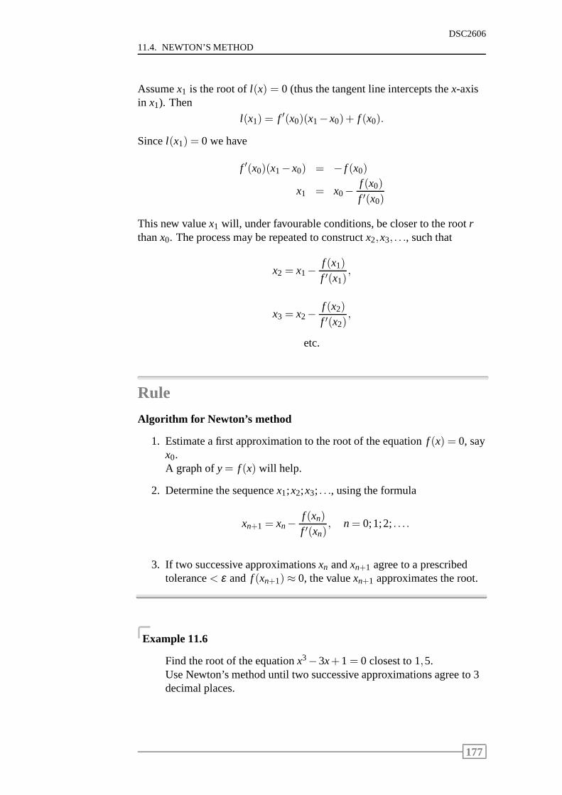
11.4. NEWTON’S METHOD
DSC2606
Assumex1 is the root ofl(x) = 0 (thus the tangent line intercepts thex-axisin x1). Then
l(x1) = f ′(x0)(x1−x0)+ f (x0).
Sincel(x1) = 0 we have
f ′(x0)(x1−x0) = − f (x0)
x1 = x0−f (x0)
f ′(x0)
This new valuex1 will, under favourable conditions, be closer to the rootrthanx0. The process may be repeated to constructx2,x3, . . ., such that
x2 = x1−f (x1)
f ′(x1),
x3 = x2−f (x2)
f ′(x2),
etc.
Rule
Algorithm for Newton’s method
1. Estimate a first approximation to the root of the equationf (x) = 0, sayx0.A graph ofy= f (x) will help.
2. Determine the sequencex1;x2;x3; . . ., using the formula
xn+1 = xn−f (xn)
f ′(xn), n= 0;1;2;. . . .
3. If two successive approximationsxn andxn+1 agree to a prescribedtolerance< ε and f (xn+1)≈ 0, the valuexn+1 approximates the root.
Example 11.6
Find the root of the equationx3−3x+1= 0 closest to 1,5.Use Newton’s method until two successive approximations agree to 3decimal places.
177
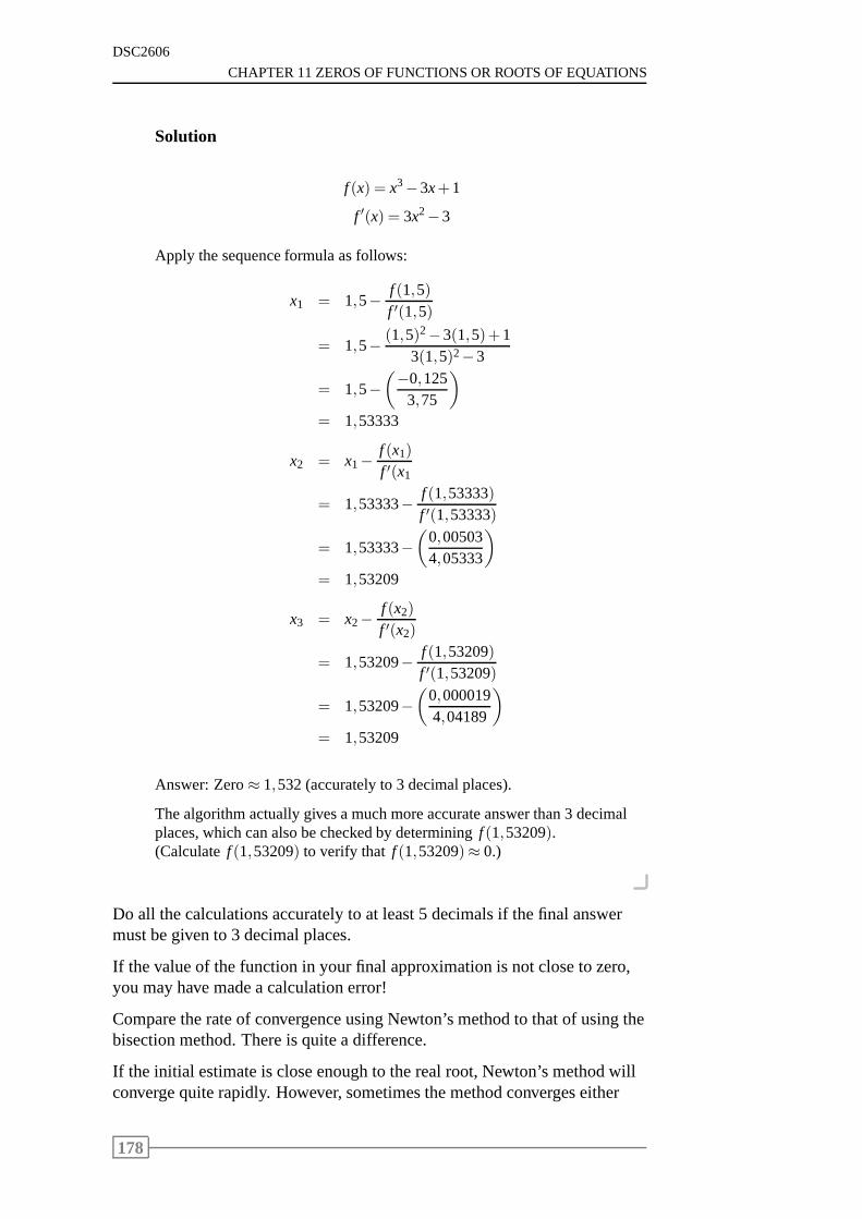
DSC2606
CHAPTER 11 ZEROS OF FUNCTIONS OR ROOTS OF EQUATIONS
Solution
f (x) = x3−3x+1
f ′(x) = 3x2−3
Apply the sequence formula as follows:
x1 = 1,5− f (1,5)f ′(1,5)
= 1,5− (1,5)2−3(1,5)+13(1,5)2−3
= 1,5−(−0,125
3,75
)
= 1,53333
x2 = x1−f (x1)
f ′(x1
= 1,53333− f (1,53333)f ′(1,53333)
= 1,53333−(
0,005034,05333
)
= 1,53209
x3 = x2−f (x2)
f ′(x2)
= 1,53209− f (1,53209)f ′(1,53209)
= 1,53209−(
0,0000194,04189
)
= 1,53209
Answer: Zero≈ 1,532 (accurately to 3 decimal places).
The algorithm actually gives a much more accurate answer than 3 decimalplaces, which can also be checked by determiningf (1,53209).(Calculatef (1,53209) to verify that f (1,53209)≈ 0.)
Do all the calculations accurately to at least 5 decimals if the final answermust be given to 3 decimal places.
If the value of the function in your final approximation is notclose to zero,you may have made a calculation error!
Compare the rate of convergence using Newton’s method to that of using thebisection method. There is quite a difference.
If the initial estimate is close enough to the real root, Newton’s method willconverge quite rapidly. However, sometimes the method converges either
178
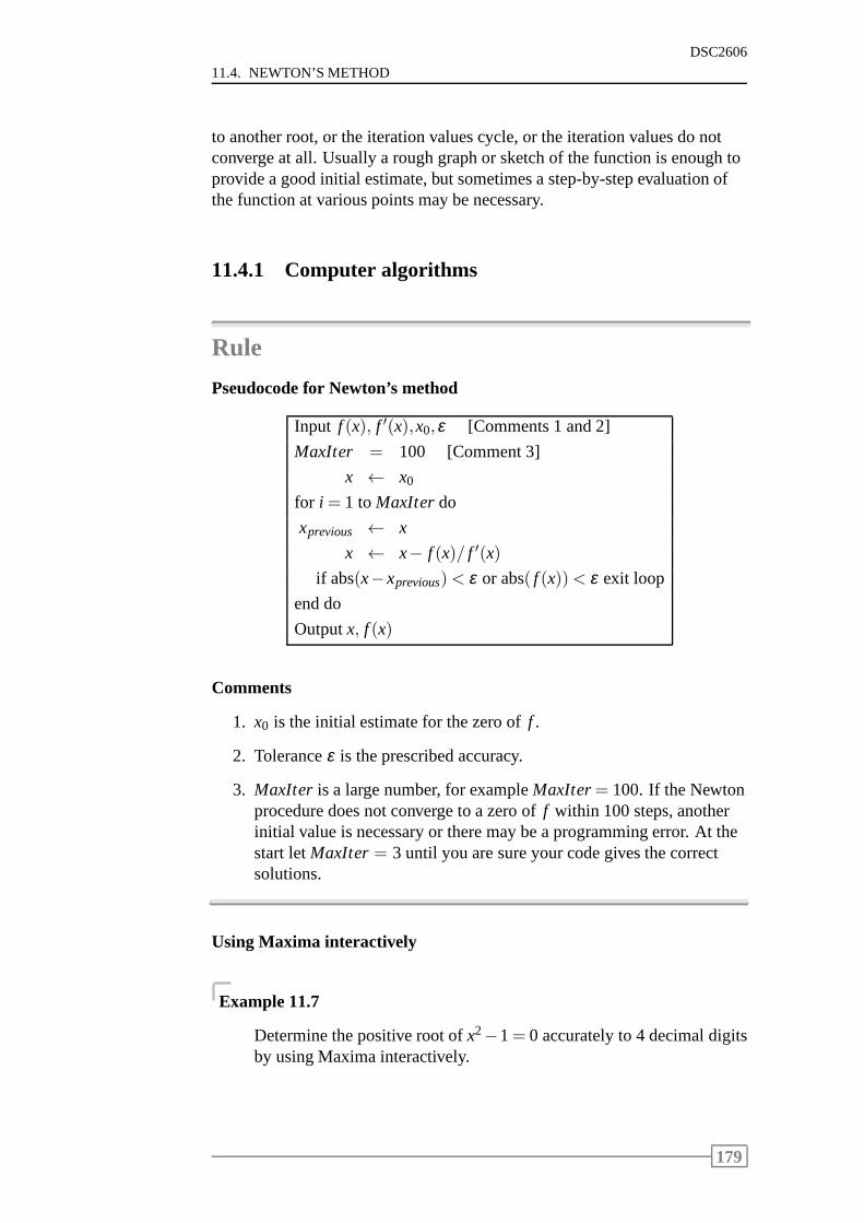
11.4. NEWTON’S METHOD
DSC2606
to another root, or the iteration values cycle, or the iteration values do notconverge at all. Usually a rough graph or sketch of the function is enough toprovide a good initial estimate, but sometimes a step-by-step evaluation ofthe function at various points may be necessary.
11.4.1 Computer algorithms
Rule
Pseudocode for Newton’s method
Input f (x), f ′(x),x0,ε [Comments 1 and 2]
MaxIter = 100 [Comment 3]
x ← x0
for i = 1 toMaxIter do
xprevious ← x
x ← x− f (x)/ f ′(x)
if abs(x−xprevious)< ε or abs( f (x))< ε exit loop
end do
Outputx, f (x)
Comments
1. x0 is the initial estimate for the zero off .
2. Toleranceε is the prescribed accuracy.
3. MaxIter is a large number, for exampleMaxIter= 100. If the Newtonprocedure does not converge to a zero off within 100 steps, anotherinitial value is necessary or there may be a programming error. At thestart letMaxIter= 3 until you are sure your code gives the correctsolutions.
Using Maxima interactively
Example 11.7
Determine the positive root ofx2−1= 0 accurately to 4 decimal digitsby using Maxima interactively.
179
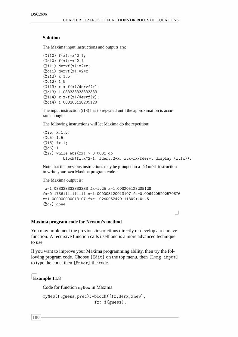
DSC2606
CHAPTER 11 ZEROS OF FUNCTIONS OR ROOTS OF EQUATIONS
Solution
The Maxima input instructions and outputs are:
(%i10) f(x):=x^2-1;
(%o10) f(x):=x^2-1
(%i11) dervf(x):=2*x;
(%o11) dervf(x):=2*x
(%i12) x:1.5;
(%o12) 1.5
(%i13) x:x-f(x)/dervf(x);
(%o13) 1.083333333333333
(%i14) x:x-f(x)/dervf(x);
(%o14) 1.003205128205128
The input instruction (i13) has to repeated until the approximation is accu-rate enough.
The following instructions will let Maxima do the repetition:
(%i5) x:1.5;
(%o5) 1.5
(%i6) fx:1;
(%o6) 1
(%i7) while abs(fx) > 0.0001 do
block(fx:x^2-1, fderv:2*x, x:x-fx/fderv, display (x,fx));
Note that the previous instructions may be grouped in a[block] instructionto write your own Maxima program code.
The Maxima output is:
x=1.083333333333333 fx=1.25 x=1.003205128205128
fx=0.17361111111111 x=1.000005120013107 fx=0.0064205292570676
x=1.000000000013107 fx=1.0240052429111302*10^-5
(%o7) done
Maxima program code for Newton’s method
You may implement the previous instructions directly or develop a recursivefunction. A recursive function calls itself and is a more advanced techniqueto use.
If you want to improve your Maxima programming ability, thentry the fol-lowing program code. Choose[Edit] on the top menu, then[Long input]
to type the code, then[Enter] the code.
Example 11.8
Code for functionmyNew in Maxima
myNew(f,guess,prec):=block([fx,derx,xnew],
fx: f(guess),
180
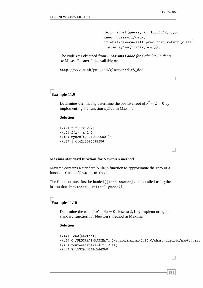
11.4. NEWTON’S METHOD
DSC2606
derx: subst(guess, x, diff(f(x),x)),
xnew: guess-fx/derx,
if abs(xnew-guess)< prec then return(guess)
else myNew(f,xnew,prec));
The code was obtained fromA Maxima Guide for Calculus Studentsby Moses Glasner. It is available on
http://www.math/psu.edu/glasner/Max$_doc
Example 11.9
Determine√
2, that is, determine the positive root ofx2− 2 = 0 byimplementing the functionmyNew in Maxima.
Solution
(%i2) f(x):=x^2-2;
(%o2) f(x):=x^2-2
(%i3) myNew(f,1.7,0.00001);
(%o3) 1.414213576599356
Maxima standard function for Newton’s method
Maxima contains a standard built-in function to approximate the zero of afunction f using Newton’s method.
The function must first be loaded ([load newton] and is called using theinstruction[newton(f, initial guess)].
Example 11.10
Determine the root ofex−4x = 0 close to 2,1 by implementing thestandard function for Newton’s method in Maxima.
Solution
(%i4) load(newton);
(%o4) C:/PROGRA~1/MAXIMA~1.0/share/maxima/5.14.0/share/numeric/newton.mac
(%i5) newton(exp(x)-4*x, 2.1);
(%o5) 2.153292364162442b0
181
DSC2606
CHAPTER 11 ZEROS OF FUNCTIONS OR ROOTS OF EQUATIONS
11.5 Exercises
1. Determine the other two roots ofx3−3x+1 = 0 using the bisectionalgorithm and Newton’s method.Do at least 3 iterations using your pocket calculator, and then use acomputer program to find a more accurate solution.Use the graph on page 172 to choose initial intervals containing a rootor to determine an initial estimate of a root.
182
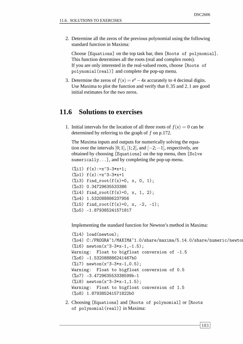
11.6. SOLUTIONS TO EXERCISES
DSC2606
2. Determine all the zeros of the previous polynomial using the followingstandard function in Maxima:
Choose[Equations] on the top task bar, then[Roots of polynomial].This function determines all the roots (real and complex roots).If you are only interested in the real-valued roots, choose[Roots of
polynomial(real)] and complete the pop-up menu.
3. Determine the zeros off (x) = ex−4x accurately to 4 decimal digits.Use Maxima to plot the function and verify that 0,35 and 2,1 are goodinitial estimates for the two zeros.
11.6 Solutions to exercises
1. Initial intervals for the location of all three roots off (x) = 0 can bedetermined by referring to the graph off on p.172.
The Maxima inputs and outputs for numerically solving the equa-tion over the intervals[0;1], [1;2], and[−2;−1], respectively, areobtained by choosing[Equations] on the top menu, then[Solvenumerically...], and by completing the pop-up menu.
(%i1) f(x):=x^3-3*x+1;
(%o1) f(x):=x^3-3*x+1
(%i3) find_root(f(x)=0, x, 0, 1);
(%o3) 0.34729635533386
(%i4) find_root(f(x)=0, x, 1, 2);
(%o4) 1.532088886237956
(%i5) find_root(f(x)=0, x, -2, -1);
(%o5) -1.879385241571817
Implementing the standard function for Newton’s method in Maxima:
(%i4) load(newton);
(%o4) C:/PROGRA~1/MAXIMA~1.0/share/maxima/5.14.0/share/numeric/newton
(%i6) newton(x^3-3*x-1,-1.5);
Warning: Float to bigfloat conversion of -1.5
(%o6) -1.532088886241467b0
(%i7) newton(x^3-3*x-1,0.5);
Warning: Float to bigfloat conversion of 0.5
(%o7) -3.472963553338599b-1
(%i8) newton(x^3-3*x-1,1.5);
Warning: Float to bigfloat conversion of 1.5
(%o8) 1.879385241571822b0
2. Choosing[Equations] and[Roots of polynomial] or [Rootsof polynomial(real)] in Maxima:
183
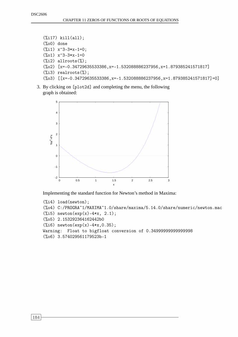
DSC2606
CHAPTER 11 ZEROS OF FUNCTIONS OR ROOTS OF EQUATIONS
(%i17) kill(all);
(%o0) done
(%i1) x^3-3*x-1=0;
(%o1) x^3-3*x-1=0
(%i2) allroots(%);
(%o2) [x=-0.34729635533386,x=-1.532088886237956,x=1.879385241571817]
(%i3) realroots(%);
(%o3) [[x=-0.34729635533386,x=-1.532088886237956,x=1.879385241571817]=0]
3. By clicking on[plot2d] and completing the menu, the followinggraph is obtained:
-2
-1
0
1
2
3
4
5
0 0.5 1 1.5 2 2.5 3
%ex -4
*x
x
Implementing the standard function for Newton’s method in Maxima:
(%i4) load(newton);
(%o4) C:/PROGRA~1/MAXIMA~1.0/share/maxima/5.14.0/share/numeric/newton.mac
(%i5) newton(exp(x)-4*x, 2.1);
(%o5) 2.153292364162442b0
(%i6) newton(exp(x)-4*x,0.35);
Warning: Float to bigfloat conversion of 0.34999999999999998
(%o6) 3.574029561179523b-1
184
Chapter 12
Marginal analysis
Contents12.1 Introduction . . . . . . . . . . . . . . . . . . . . . . . . 186
12.2 Cost functions . . . . . . . . . . . . . . . . . . . . . . . 186
12.3 Average cost functions . . . . . . . . . . . . . . . . . . . 189
12.4 Revenue functions . . . . . . . . . . . . . . . . . . . . . 192
12.5 Profit functions . . . . . . . . . . . . . . . . . . . . . . . 194
12.6 Exercises . . . . . . . . . . . . . . . . . . . . . . . . . . 195
12.7 Solution to exercises . . . . . . . . . . . . . . . . . . . . 195
185
DSC2606
CHAPTER 12 MARGINAL ANALYSIS
Learning objectivesAfter completing this study unit you should be able to
• explain the concepts of marginal analysis, cost, revenue and profit
• derive the revenue function from a demand function
• derive the profit function
• determine the marginal cost, marginal revenue and marginalprofitfunctions, and explain their meaning
• determine the average cost function and the marginal average costfunction, and explain their meaning
• use differential calculus to solve marginal analysis problems.
12.1 Introduction
Marginal analysis is the study of the rate of change of economic quanti-ties. For example, an economist is not merely concerned withthe value ofan economy’s gross domestic product (GDP) at a given time, but is equallyconcerned with the rate at which it is growing or declining. In the same vein,a manufacturer is not only interested in the total cost corresponding to a cer-tain level of production of a commodity, but is also interested in the rate ofchange of the total cost with respect to the level of production, and so on.
12.2 Cost functions
The total weekly cost (in rand) incurred by the Polarair Company is given by
C(x) = 8000+200x−0,2x2 for 0≤ x≤ 400,
wherex represents the number of refrigerators produced per week.
Suppose we want to know how much it actually costs to produce the 251strefrigerator. This can be found by calculating the difference between thetotal cost of producing the first 251 and the total cost of producing the first250 refrigerators, as follows:
C(251)−C(250) = [8000+200(251)−0,2(251)2]− [8000+200(250)−0,2(250)2]
= 45599,8−45500
= R99,80.
Now, if we want to know how fast total cost will change with respect to pro-duction, we have to find the derivative ofC(x). Then
C′(x) = 200−0,4x.
186
12.2. COST FUNCTIONS
DSC2606
This is the rate of change of the total cost functionC(x) with respect tox.
At a level of production of 250 refrigerators, we have
C′(250) = 200−0,4(250) = R100.
This means that total cost is increasing at a rate of R100 per refrigeratorwhen 250 refrigerators are produced, which in turn implies that the next re-frigerator will actually cost R100 to produce.
Let us now compare these two results.
The differenceC(251)−C(250) may be written in the form
C(251)−C(250)1
=C(250+1)−C(250)
1
=C(250+h)−C(250)
h,
whereh = 1. This is the average rate of change of the total cost functionC(x) over the interval[250;251]. On the other hand,C′(250) is the instanta-neous rate of change ofC(x) at x= 250.
Now, whenh is very small, the average rate of change of the functionC(x) isa good approximation of the instantaneous rate of change ofC(x).
We can therefore say that
C(250+h)−C(250)h
≈ limh→0
C(250+h)−C(250)h
=C′(250),
which means thatC′(250) also approximates the actual cost incurred in pro-ducing the 251st refrigerator.
This gives rise to the following definition:
Definition 12.1 Themarginal cost functionat a particular point is the deriva-tive of the total cost function evaluated at that point, and this gives the actualcost incurred in producing an additional unit, given that production is at alevel corresponding to the point under consideration.
From this definition it follows that the marginal cost function,C′(x), eval-uated at pointx, provides us with a good approximation of the actual costincurred in producing the(x+ 1)st unit of a product, assuming thatx unitsare already produced.
Example 12.1
187
DSC2606
CHAPTER 12 MARGINAL ANALYSIS
A subsidiary of the Elektra Electronics Company manufactures a pro-grammable pocket calculator. The daily total cost (in rand)of produc-ing these calculators is given by
C(x) = 0,0001x3−0,08x2+40x+5000,
wherex represents the number of calculators produced.
(a) Find the marginal cost function.
(b) Calculate the marginal cost forx=100, 200, 300, 400, 600 and 700.
(c) Interpret the results.
Solution
(a) The marginal cost function is given by the derivative of the total costfunction
C′(x) = 0,0003x2−0,16x+40.
(b) The required marginal costs are
C′(100) = 0,0003(100)2−0,16(100)+40= 27
C′(200) = 0,0003(200)2−0,16(200)+40= 20
C′(300) = 19
C′(400) = 24
C′(600) = 52
C′(700) = 75.
(c) The actual cost of producing an additional calculator ata certain pro-duction level is the marginal cost and this is given by the derivative ofthe total cost function at this production level. We see thatthe actualcost incurred in producing one additional calculator at a productionlevel of 100 calculators, is R27; at a production level of 200calcula-tors, it is R20, and so on.
The actual cost of producing an additional calculator dropsat first asthe production level increases. This is true up to a production level ofbetween 300 and 400 calculators. Thereafter the actual costof produc-ing an additional unit increases.
Observe that at a production level of 700 calculators, the actual costof producing one additional calculator is R75. The higher cost of pro-ducing one additional unit at this production level may be the result ofseveral factors, among them excessive costs incurred because of over-time or higher maintenance, production breakdown caused bygreaterstress and strain on equipment, and so on.
188
12.3. AVERAGE COST FUNCTIONS
DSC2606
12.3 Average cost functions
Let us now introduce another marginal concept closely related to the marginalcost. IfC(x) denotes the total cost incurred in producingx units of a certainproduct, then the average cost of producingx units of the product is obtainedby dividing the total production cost by the number of units produced.
Definition 12.2 The average cost of producing one unit of a product isgiven by the function
C(x) =C(x)
x,
whereC(x) is the total cost of producingx units.C(x) is called theaveragecost function.
The marginal average cost function,C′(x), measures the rate of change of
the average cost function with respect to the number of unitsproduced. Thismeans that the average cost function gives the average cost of producingone unit of a product and the marginal average cost function gives the rate atwhich this average cost changes.
Example 12.2
The total cost (in rand) of producingx units of a certain product isgiven by
C(x) = 400+20x.
(a) Find the average cost function.
(b) Find the marginal average cost function.
(c) Interpret the results obtained in (a) and (b).
Solution
(a) The average cost function is given by
C(x) =C(x)
x
=400+20x
x
= 20+400x
.
(b) The marginal average cost function isC′(x) =−400
x2 .
189
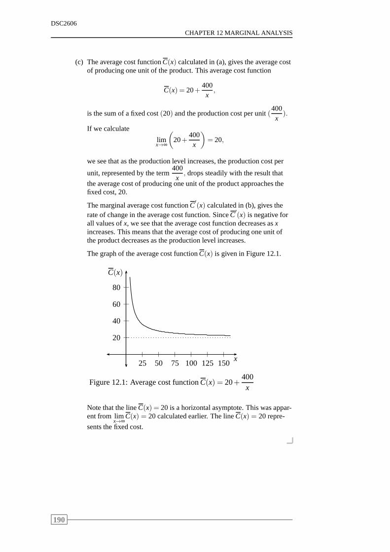
DSC2606
CHAPTER 12 MARGINAL ANALYSIS
(c) The average cost functionC(x) calculated in (a), gives the average costof producing one unit of the product. This average cost function
C(x) = 20+400x
,
is the sum of a fixed cost(20) and the production cost per unit(400x
).
If we calculate
limx→∞
(
20+400x
)
= 20,
we see that as the production level increases, the production cost per
unit, represented by the term400x
, drops steadily with the result that
the average cost of producing one unit of the product approaches thefixed cost, 20.
The marginal average cost functionC′(x) calculated in (b), gives the
rate of change in the average cost function. SinceC′(x) is negative for
all values ofx, we see that the average cost function decreases asxincreases. This means that the average cost of producing oneunit ofthe product decreases as the production level increases.
The graph of the average cost functionC(x) is given in Figure 12.1.
20
40
60
80
25 50 75 100 125 150x
C(x)
Figure 12.1: Average cost functionC(x) = 20+400x
Note that the lineC(x) = 20 is a horizontal asymptote. This was appar-ent from lim
x→∞C(x) = 20 calculated earlier. The lineC(x) = 20 repre-
sents the fixed cost.
190
12.3. AVERAGE COST FUNCTIONS
DSC2606
Example 12.3
Once again consider the subsidiary of the Elektra Electronics Com-pany. The daily total cost (in rand) of producing its programmablecalculators is given by
C(x) = 0,0001x3−0,08x2+40x+5000,
wherex represents the number of calculators produced.
(a) Find the marginal average cost function and calculateC′(500).
(b) Interpret the results obtained in (a).
Solution
(a) The average cost function is
C(x) =C(x)
x
= 0,0001x2−0,08x+40+5000
x.
The marginal average cost function is
C′(x) = 0,0002x−0,08− 5000
x2 .
Therefore
C′(500) = 0,0002(500)−0,08− 5000
(500)2 = 0.
(b) The fact thatC′(500)= 0 means that the average cost functionC(x) has
a critical point atx= 500.
The second derivative ofC(x) is
C′′(x) = 0,0002+
5000x3 .
Evaluating the second derivative atx= 500 gives
C′′(500) = 0,00024> 0⇒ relative minimum.
Now atx= 500, the value of the average cost function is
C(500) = 0,0001(500)2−0,08(500)+40+5000500
= 35.
The point(500;35) is a relative minimum point ofC(x).
191
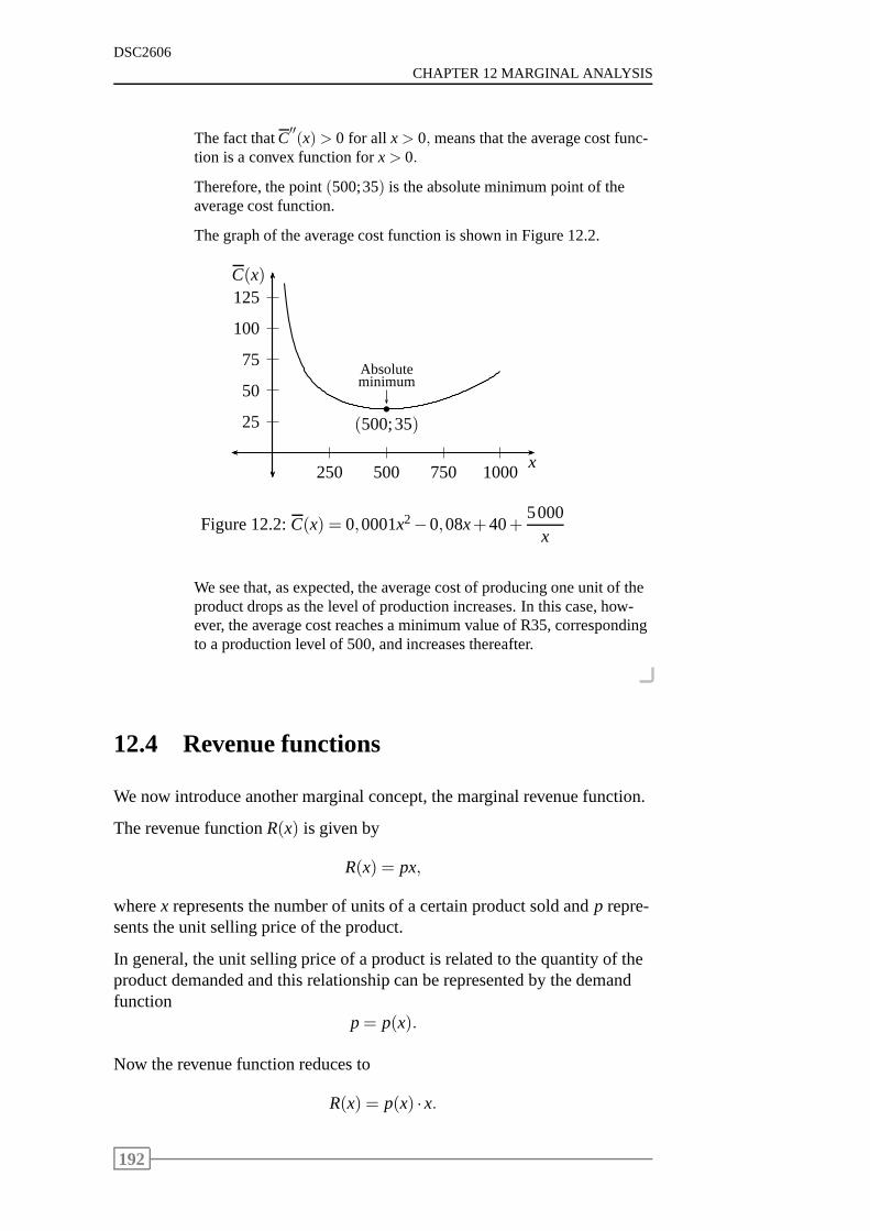
DSC2606
CHAPTER 12 MARGINAL ANALYSIS
The fact thatC′′(x)> 0 for all x> 0, means that the average cost func-
tion is a convex function forx> 0.
Therefore, the point(500;35) is the absolute minimum point of theaverage cost function.
The graph of the average cost function is shown in Figure 12.2.
25
50
75
100
125
250 500 750 1000x
C(x)
b
(500;35)
minimumAbsolute
Figure 12.2:C(x) = 0,0001x2−0,08x+40+5000
x
We see that, as expected, the average cost of producing one unit of theproduct drops as the level of production increases. In this case, how-ever, the average cost reaches a minimum value of R35, correspondingto a production level of 500, and increases thereafter.
12.4 Revenue functions
We now introduce another marginal concept, the marginal revenue function.
The revenue functionR(x) is given by
R(x) = px,
wherex represents the number of units of a certain product sold andp repre-sents the unit selling price of the product.
In general, the unit selling price of a product is related to the quantity of theproduct demanded and this relationship can be represented by the demandfunction
p= p(x).
Now the revenue function reduces to
R(x) = p(x) ·x.
192
12.4. REVENUE FUNCTIONS
DSC2606
The derivative,R′(x), of the revenue function is called the marginal revenuefunction and it measures the rate of change of the revenue function with re-spect to the number of units demanded.
A definition for marginal revenue follows easily from the definition formarginal cost given in Section 12.2.
Definition 12.3 Themarginal revenue functionat a particular point is thederivative of the revenue function evaluated at that point,and this gives theactual revenue earned from selling an additional unit, given that sales arealready at a level corresponding to the point under consideration.
The marginal revenue function,R′(x), evaluated at pointx, provides us witha good approximation of the actual revenue earned from the sale of the(x+1)st unit of a product, assuming thatx units have already been sold.
Example 12.4
The relationship between the unit pricep (in rand) and the quantitydemandedx of the Acrosonic modelF loudspeaker system is given bythe function
p(x) =−0,02x+400 for 0≤ x≤ 20000.
(a) Find the revenue function.
(b) Find the marginal revenue function.
(c) CalculateR′(2000) and explain the meaning of this.
Solution
(a) The revenue function is
R(x) = p(x) ·x= (−0,02x+400) ·x= −0,02x2+400x.
(b) The marginal revenue function isR′(x) =−0,04x+400.
(c) The required calculation isR′(2000) =−0,04(2000)+400= 320.
This means that the actual revenue earned from the sale of the2001stloudspeaker system is approximately R320.
193
DSC2606
CHAPTER 12 MARGINAL ANALYSIS
12.5 Profit functions
Since profit is calculated as the difference between revenueand cost, it isobvious that the profit functionP(x) is given by
P(x) = R(x)−C(x),
whereR(x) is the revenue function,C(x) is the cost function andx representsthe number of units of a product produced and sold.
The marginal profit function,P′(x), measures the rate of change of the profitfunctionP(x).
Definition 12.4 Themarginal profit functionat a particular point is thederivative of the profit function evaluated at that point, and this gives theactual profit realised from selling an additional unit, given that sales are al-ready at a level corresponding to the point under consideration.
The marginal profit function,P′(x), evaluated at pointx, provides us with agood approximation of the actual profit or loss realised fromthe sale of the(x+1)st unit of a product, assuming thatx units have already been sold.
Example 12.5
Refer to example 12.4. Suppose that the cost (in rand) of producingxunits of the Acrosonic modelF loudspeaker isC(x) = 100x+200000.
(a) Find the profit function.
(b) Find the marginal profit function.
(c) CalculateP′(2000) and explain the meaning of this.
Solution
(a) The revenue function was calculated as
R(x) =−0,02x2+400x.
The required profit function is
P(x) = R(x)−C(x)
= −0,02x2+400x− (100x+200000)
= −0,02x2+300x−200000.
(b) The marginal profit function isP′(x) =−0,04x+300.
(c) The required calculation isP′(2000) =−0,04(2000)+300= 220.
This means that the actual profit realised from the sale of the2001stloudspeaker system is approximately R220.
194
12.6. EXERCISES
DSC2606
12.6 Exercises
1. The weekly demand for Pulsar VCRs (videocassette recorders) isgiven by the demand function
p=−0,02x+300 for 0≤ x≤ 15000,
wherep represents the wholesale unit price in rand andx representsthe quantity demanded.
The weekly total cost function (in rand) associated with manufacturingthese VCRs is given by
C(x) = 0,000003x3−0,04x2+200x+70000.
(a) Find the revenue function and the profit function.
(b) Find the marginal cost function, the marginal revenue function,and the marginal profit function.
(c) Calculate the marginal cost function, the marginal revenue func-tion and the marginal profit function at the pointx = 3000 andexplain the results.
(d) Calculate the marginal cost function at pointsx= 30 andx= 300and compare these results with the result of the marginal costfunction evaluated atx= 3000 in (c) above.
(e) Find the average cost function and the marginal average costfunction.
(f) Calculate the average cost function and the marginal average costfunction at pointx= 3000 and explain the results.
12.7 Solution to exercises
1. (a) The revenue function is
R(x) = px
= (−0,02x+300) ·x= −0,02x2+300x.
The profit function is
P(x) = R(x)−C(x)
= −0,02x2+300x− (0,000003x3−0,04x2+200x+70000)
= −0,000003x3+0,02x2+100x−70000.
195
DSC2606
CHAPTER 12 MARGINAL ANALYSIS
(b) The marginal functions are
C′(x) = 0,000009x2−0,08x+200
R′(x) = −0,04x+300
P′(x) = −0,000009x2+0,04x+100.
(c) The marginal cost function evaluated atx= 3000 is
C′(3000) = 0,000009(3000)2−0,08(3000)+200= 41.
The marginal revenue function evaluated atx= 3000 is
R′(3000) =−0,04(3000)+300= 180.
The marginal profit function evaluated atx= 3000 is
P′(3000) =−0,000009(3000)2+0,04(3000)+100= 139.
This means that at a production level of 3000 VCRs, the actualcost of producing one additional unit is approximately R41, theactual revenue from selling the 3001st VCR is approximatelyR180 and the actual profit from selling the 3001st VCR is R139.
(d) The marginal cost function evaluated atx= 30 is
C′(30) = 0,000009(30)2−0,08(30)+200= 197,61.
The marginal cost function evaluated atx= 300 is
C′(300) = 176,81.
From (c), the marginal cost function evaluated atx = 3000 was41.
This means that the cost of producing an additional VCR is R197,61at a production level of 30; is R176,81 at a production level of300; and R41 at a production level of 3000.
This illustrates clearly that the cost of producing an additionalVCR decreases as the production level increases from 30 to 3000units.
(e) The average cost function is
C(x) =C(x)
x
= 0,000003x2−0,04x+200+70000
x.
The marginal average cost function is
C′(x) = 0,000006x−0,04− 70000
x2 .
196
12.7. SOLUTION TO EXERCISES
DSC2606
(f) The average cost function evaluated atx= 3000 is
C(3000)=0,000003(3000)2−0,04(3000)+200+700003000
=130,33.
The marginal average cost function evaluated atx= 3000 is
C′(3000) = 0,000006(3000)−0,04− 70000
(3000)2 =−0,03.
This means that if 3000 VCRs have already been produced, theaverage cost of producing one such VCR is R130,33 and theaverage cost of producing one VCR is decreasing at the rate ofR0,03 per unit.
197

DSC2606
CHAPTER 12 MARGINAL ANALYSIS
198
Chapter 13
Optimisation of NLPs in onevariable
Contents13.1 Introduction . . . . . . . . . . . . . . . . . . . . . . . . 200
13.2 Vital theorems . . . . . . . . . . . . . . . . . . . . . . . 200
13.3 Solving NLPs in one variable by differential calculus .. 201
13.4 Returning to LINGO . . . . . . . . . . . . . . . . . . . 206
13.5 Exercises . . . . . . . . . . . . . . . . . . . . . . . . . . 207
13.6 Solutions to exercises . . . . . . . . . . . . . . . . . . . 208
199
DSC2606
CHAPTER 13 OPTIMISATION OF NLPS IN ONE VARIABLE
Learning objectivesAfter completing this study unit you should be able to
• solve NLPs in one variable by means of differential calculus
• test whether the solution obtained by means of differentialcalculus isindeed the optimal solution to the NLP
• test whether the solution obtained by means of LINGO is indeed theoptimal solution to the NLP.
13.1 Introduction
In this study guide we see that real-world problems can be represented asmodels, and these models may be LP or NLP models depending on thenature of the problem. Various techniques are used to find solutions to themodels. In Part 1 of the study guide we used the graphical method to solveLP models. We used the computer, specifically the LINGO package, to sim-plify this solution process.
In Study unit 6 we used the LINGO computer package to solve NLPmod-els. We warned that the solution thus obtained is not necessarily the optimalsolution and that certain criteria must apply before we may conclude thatthe solution is optimal. We needed more information on functions and theirproperties and turned to differential calculus for this.
Winstongives the criteria necessary for a solution to be the optimalsolutionto an NLP model. This is related to the concavity of functionsand is givenin two theorems. These theorems are of the utmost importanceand are there-fore repeated in the next section.
13.2 Vital theorems
Theorem 13.1 If we are maximising a concave function over a convex do-main, then any local maximum point will be the absolute maximum point ofthe function, and therefore the optimal solution.
Theorem 13.2 If we are minimising a convex function over a convex do-main, then any local minimum point will be the absolute minimum point ofthe function, and therefore the optimal solution.
200
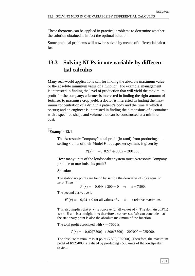
13.3. SOLVING NLPS IN ONE VARIABLE BY DIFFERENTIAL CALCULUS
DSC2606
These theorems can be applied in practical problems to determine whetherthe solution obtained is in fact the optimal solution.
Some practical problems will now be solved by means of differential calcu-lus.
13.3 Solving NLPs in one variable by differen-tial calculus
Many real-world applications call for finding the absolute maximum valueor the absolute minimum value of a function. For example, managementis interested in finding the level of production that will yield the maximumprofit for the company; a farmer is interested in finding the right amount offertiliser to maximise crop yield; a doctor is interested infinding the max-imum concentration of a drug in a patient’s body and the time at which itoccurs; and an engineer is interested in finding the dimensions of a containerwith a specified shape and volume that can be constructed at a minimumcost.
Example 13.1
The Acrosonic Company’s total profit (in rand) from producing andsellingx units of their ModelF loudspeaker systems is given by
P(x) =−0,02x2+300x−200000.
How many units of the loudspeaker system must Acrosonic Companyproduce to maximise its profit?
Solution
The stationary points are found by setting the derivative ofP(x) equal tozero. Then
P′(x) =−0,04x+300= 0 ⇒ x= 7500.
The second derivative is
P′′(x) =−0,04< 0 for all values ofx ⇒ a relative maximum.
This also implies thatP(x) is concave for all values ofx. The domain ofP(x)is x ∈ R and is a straight line; therefore a convex set. We can conclude thatthe stationary point is also the absolute maximum of the function.
The total profit associated withx= 7500 is
P(x) =−0,02(7500)2+300(7500)−200000= 925000.
The absolute maximum is at point(7500;925000). Therefore, the maximumprofit of R925000 is realised by producing 7500 units of the loudspeakersystem.
201
DSC2606
CHAPTER 13 OPTIMISATION OF NLPS IN ONE VARIABLE
The graph ofP(x) in Figure 13.1 (wherex is measured in thousands of unitsandP(x) is measured in thousands of rand) confirms these findings.
200
400
600
800
1000
−200 5 10 15x
P(x)
bAbsolute maximum= (7,5;925)
Figure 13.1: Acrosonic Company’s profit function
Example 13.2
The present value of the market price of the Blakely Office Building attime t is given by
P(t) = 300000e(−0,09t+√
t2 ) for 0≤ t ≤ 10.
Find the optimal present value of the market price of the building.
Solution
The derivative is
P′(t) = 300000e(−0,09t+√
t2 ) d
dt
(
−0,09t +12
t12
)
= 300000e(−0,09t+√
t2 )
(
−0,09+14
t−12
)
.
The stationary points follow from settingP′(t) = 0. Sincee(−0,09t+√
t2 ) is
never zero for any value oft, we must have
−0,09+1
4t12
= 0.
202

13.3. SOLVING NLPS IN ONE VARIABLE BY DIFFERENTIAL CALCULUS
DSC2606
Solving this equation, we find
1
4t12
= 0,09
t12 =
14(0,09)
t =
(
10,36
)2
= 7,72.
And the stationary point occurs att = 7,72.
We evaluateP(t) at the stationary point as well as at the endpoints of[0;10]:
t P(t)0 300 000
7,72 600 77910 592 838
We conclude, accordingly, that the optimal present value ofthe market priceof the building is R600779 and this will occur 7,72 years from now.
In the previous examples the functions to be optimised were given. Now,we consider a problem where we are required to first find the appropriatefunction. Once the function has been found, it may be optimised.
The annual total cost function (in rand) of a maize farmer is given by
C(x) =x2
10+10000,
wherex is the number of tons of mealies produced. Mealies are sold atR250per ton.
Obviously, the farmer wants to maximise his profit.
If the farmer producesx tons of mealies per year, his revenue is given by
R(x) = p ·x= 250x.
Now, his profit function is given by
profit = revenue−cost
P(x) = R(x)−C(x)
= 250x−(
x2
10+10000
)
= − x2
10+250x−10000.
203
DSC2606
CHAPTER 13 OPTIMISATION OF NLPS IN ONE VARIABLE
To find the value ofx that will maximiseP(x), we set the derivative of theprofit function equal to zero. Then
P′(x) = −x5+250= 0
x5
= 250
x = 1250.
To determine whether this point is a maximum, we use the second deriva-tive. Then
P′′(x) =−15< 0 for all x ⇒ relative maximum.
This also indicates thatP(x) is a concave function for all values ofx andwe can conclude that the stationary point is the absolute maximum of thefunction.
Profit is therefore indeed a maximum at the production level of 1250 tons.
The maximum profit is
P(1250) = −(1250)2
10+250(1250)−10000
= R146250.
In general, we can say that for maximum profit
P′(x) = R′(x)−C′(x) = 0 ⇒ R′(x) =C′(x),
which meansmarginal revenue= marginal cost.
This is the basis for the classical economic criterion whichstates thatifmarginal revenue equals marginal cost, profit is a maximum.Beyond thispoint (ie for largerx values) the cost of producing additional units exceedsthe revenue derived from the extra units.
The maize farmer’s problem can also be solved using this criterion. We have
R(x) = 250x ⇒ R′(x) = 250
C(x) =x2
10+10000 ⇒ C′(x) =
x5.
For maximum profit
R′(x) = C′(x)
250 =x5
x = 1250 tons.
In Study unit 6 we modelled two problems; a dimensions of a boxproblemand an inventory problem. And we solved them with LINGO. Let us nowsee how these models are solved with differential calculus.
204

13.3. SOLVING NLPS IN ONE VARIABLE BY DIFFERENTIAL CALCULUS
DSC2606
Example 13.3
Return to Section 6.2 for the dimensions problem. The NLP modelfound there is
Maximise V(x) = 4(x3−13x2+40x)
subject to 0≤ x≤ 5.
The derivatives are
V ′(x) = 4(3x2−26x+40)
V ′′(x) = 4(6x−26).
Now the stationary points follow from settingV ′(x) = 0. Then
4(3x2−26x+40) = 0
4(3x−20)(x−2) = 0
x=203
andx = 2
x= 6,67 andx = 2.
The pointx = 6,67 lies outside the interval[0;5]: so it is discarded.Therefore, the stationary point is atx= 2.
Now, the second derivative atx= 2 is
V ′′(2) = 4[6(2)−26] = 4(−14) =−56< 0 ⇒ maximum point.
Therefore, a relative maximum exists atx= 2.
To determine the absolute maximum, we must evaluate the function atthe stationary point and at the endpoints. However, since the endpointsof the interval[0;5] are not feasible solutions (we will not have a boxif x = 0 orx = 5), we conclude that the stationary pointx = 2 is theabsolute maximum.
The dimensions of the box will then be
length = 16−2x= 16−2(2) = 12cm
width = 10−2x= 6cm
height = 2cm.
The maximum volume will be
V(2) = 4[23−13(2)2+40(2)] = 144cm3.
205
DSC2606
CHAPTER 13 OPTIMISATION OF NLPS IN ONE VARIABLE
Example 13.4
Return to Section 6.3 for the inventory problem. The NLP modelfound there is
Minimise C(x) = 100000000x−1+100x
subject to 0≤ x≤ 10000.
The derivatives are
C′(x) = −100000000x−2+100
C′′(x) = 200000000x−3.
Now the stationary points follow from settingC′(x) = 0. Then
−100000000x2 +100 = 0
100x2 = 100000000
x2 = 1000000
x = ±1000.
Sincex= −1000 is outside the domain of the functionC(x), it is dis-carded andx= 1000 is then the only stationary point.
Now sinceC′′(x) > 0 for all x> 0, we can deduce thatC′′(1000)> 0;thereforex= 1000 is a relative minimum point.
Also sinceC′′(x) > 0, the functionC(x) is convex forx> 0; thereforex= 1000 is the absolute minimum point ofC(x).
Therefore, the order size should be 1000 and the number of orders peryear should be
demandorder size
=100001000
= 10.
The accompanying cost will be
C(1000) =100000000
1000+100(1000)
= R200000.
13.4 Returning to LINGO
We now use the inventory problem to compare the solutions obtained bymeans of differential calculus and by means of LINGO (in Study unit 6).
206

13.5. EXERCISES
DSC2606
Both methods yielded R200000 as the minimum cost and this is obtained byhaving 1000 motorcycles in each order.
When solving by means of differential calculus, we tested that the solutionobtained was indeed the optimal solution. At the time of solving the problemby means of LINGO, we accepted the solution and were warned that it mightnot be optimal. Subsequently we have acquired the skills needed to test thesolution and will now proceed to do so.
By using theorem 17.2, we can conclude that the LINGO solution is optimalif we can show that the function to be optimised,
C(x) = 100000000x−1+100x,
is a convex function on a convex domain[0;10000].
The interval[0;10000] is a straight line betweenx= 0 andx= 10000 and istherefore a convex set.
The derivatives ofC(x) are
C′(x) = −100000000x−2+100
C′′(x) = 200000000x−3.
SinceC′′(x) > 0 for all x> 0, we conclude thatC(x) is a convex function forx> 0; therefore forx∈ [0;10000].
We have now shown thatC(x) is a convex function on a convex domain.Therefore, it follows that the solution obtained is the optimal solution.
NOTE: You must know whether the solution obtained for an NLP is theop-timal solution to the problem or not. To make this deduction you must testwhether the criteria of theorem 17.1 (or theorem 17.2) applies.
13.5 Exercises
1. The operating rate (expressed as a percentage) of factories, mines andutilities in a certain region of the country on thetth day of the year2003 is given by the function
f (t) = 80+1200t
t2+40000for 0≤ t ≤ 250.
On which day of the first 250 days of 2003 was the operating ratethehighest? (You may assume thatf (t) is a concave function on[0;250].
2. Ship Shape produces small cabin cruisers; the Neptune. The cost func-tion is given by
C(x) = 100000+6000x+4x2,
207
DSC2606
CHAPTER 13 OPTIMISATION OF NLPS IN ONE VARIABLE
wherex is the number of Neptunes produced per year. The unit priceof a Neptune is related to demand by the following demand function:
p(x) = 30000−2x.
How many Neptunes should be produced to maximise profit? Findthemaximum annual profit and the optimal selling price.
3. Titan Tyres produces a certain brand of tyres. The set-up cost for eachof their production runs is R4000. The production cost per tyre isR20. The annual storage cost per tyre is R2. The annual demandforthe tyres is 1000000.
Assuming uniformity of demand throughout the year and instanta-neous production, determine how many tyres should be manufacturedper production run in order to keep the total annual costs to amini-mum.
13.6 Solutions to exercises
1. The first derivative is
f ′(t) = 1200tddt
[
(t2+40000)−1]+(t2+40000)−1 ddt(1200t)
= 1200t(−1)(t2+40000)−2(2t)+(t2+40000)−1(1200)
=−2400t2
(t2+40000)2 +1200
(t2+40000)
=−2400t2+1200(t2+40000)
(t2+40000)2
=1200(−t2+40000)
(t2+40000)2 .
The stationary points follows fromf ′(t) = 0. Then
1200(−t2+40000)(t2+40000)2 = 0
−t2+40000 = 0
t2 = 40000
t = ±200.
Sincet = −200 is outside the domain of the functionf (t), the onlystationary point is atx= 200.
It is given thatf (t) is a concave function on[0;250]. Therefore, it fol-lows thatx= 200 is a maximum point.
208
13.6. SOLUTIONS TO EXERCISES
DSC2606
The function is now evaluated at the end points of the interval and atthe stationary point. Then
f (0) = 80
f (200) = 80+1200(200)
2002+40000= 83
f (250) = 82,93.
From this follows that the point(200;83) is the absolute maximum off (t).
We conclude that the operating rate is at its highest, 83%, onthe 200thday of 2003.
2. The marginal cost function isC′(x) = 6000+8x.
The revenue function is
R(x) = p(x) ·x= (30000−2x)x
= 30000x−2x2.
The marginal revenue function isR′(x) = 30000−4x.
For maximum profit, we must have
C′(x) = R′(x)
6000+8x = 30000−4x
12x = 24000
x = 2000.
The optimal selling price can be calculated from the demand functionas
p(2000) = 30000−2(2000)
= 26000.
The profit function is
P(x) = R(x)−C(x)
= 30000x−2x2− (100000+6000x+4x2)
= −6x2+24000x−100000,
and evaluated atx= 2000 gives
P(2000) = −6(2000)2+24000(2000)−100000
= 23900000.
209
DSC2606
CHAPTER 13 OPTIMISATION OF NLPS IN ONE VARIABLE
We conclude that Ship Shape should produce 2000 Neptunes peryearand sell them for R26000 each, and the maximum profit realisedwillbe R23,9 million.
3. Letx denote the number of tyres produced per production run.
The annual demand is 1000000 tyres and this demand must be met.
The number of production runs per year is therefore
total demand per yearnumber of tyres produced per production run
=1000000
x.
The total annual cost is
set-up cost+production cost+storage cost.
Set-up cost
The set-up cost per production run is R4 000. Therefore, the annualset-up cost is
4000× the number of runs= 4000
(
1000000x
)
=4000000000
x.
Production cost
The production cost per tyre is R20. Therefore, the production cost perproduction run is 20x and the annual production cost is
20x× the number of runs= 20x
(
1000000x
)
= 20000000
OR20×demand= 20×1000000= 20000000.
Storage cost
The number of tyres produced per production run isx and so the av-
erage number of tyres in storage isx2
. This is the average number of
tyres in storage during the year.
The storage cost is R2 per tyre and annual storage cost is therefore
2× x2= x.
The total annual cost is
C(x) =4000000000
x+20000000+x
= 4000000000x−1+20000000+x.
210
13.6. SOLUTIONS TO EXERCISES
DSC2606
NowC′(x) =−4000000000x−2+1.
Stationary points follow fromC′(x) = 0, that is,
−4000000000x2 +1 = 0
x2 = 4000000000
x = ±63245,55
≈ 63246 (ignore negative root).
NowC′′(x) = 8000000000x−3 > 0 for all x> 0.
Therefore,C is convex for allx > 0 andx = 63246 is the absoluteminimum ofC.
The company should manufacture 63 246 tyres in each of the1000000
63246= 15,8≈ 16
production runs during the year.
The minimum annual cost is
C(63245) =4000000000
63246+20000000+63246
= R20126491,11.
211

DSC2606
CHAPTER 13 OPTIMISATION OF NLPS IN ONE VARIABLE
212
Chapter 14
Golden section search
Contents14.1 Introduction . . . . . . . . . . . . . . . . . . . . . . . . 214
14.2 The golden section search . . . . . . . . . . . . . . . . . 214
14.3 Exercises . . . . . . . . . . . . . . . . . . . . . . . . . . 219
14.4 Solutions to exercises . . . . . . . . . . . . . . . . . . . 219
213
DSC2606
CHAPTER 14 GOLDEN SECTION SEARCH
Sections from prescribed book,WinstonChapter 11, Section 11.5
Learning objectivesAfter completing this study unit you should be able to
• determine whether a function is unimodal
• use the golden section search to optimise a unimodal function of onevariable.
14.1 Introduction
It may, for various reasons, be difficult to solve an NLP modelby means ofdifferential calculus and in such cases alternative solution techniques mustbe used.
In this study unit we concentrate on NLP models where the function to beoptimised is a special type of function, namely a unimodal function. We thensolve such models by means of thegolden section search, a solution tech-nique that uses a search algorithm as basis.
14.2 The golden section search
Consider the following NLP model:
Maximise z= f (x)
subject to a≤ x≤ b.
The golden section search can be used to solve this model if the objectivefunctionz is aunimodal function. The unimodality of the function is re-quired to ensure that the interval[a;b] contains only one local maximum.
StudyWinston, Section 11.5 for a description of the golden section searchtechnique (omit the section on spreadsheets). Refer to Tutorial Letter 101 forthe exact page references.
The strategy behind the golden section search is to obtain successive inter-vals of uncertainty, each smaller than the previous one. Thegolden sectionsearch is based on an algorithm that is repeated until the required accuracy isobtained.
The golden section search involves the following two steps:
214
14.2. THE GOLDEN SECTION SEARCH
DSC2606
Step 1: Let [L;R] be an interval of uncertainty. (We usually chooseL = aandR= b for the first iteration. The symbolL refers to the leftendpoint of the interval andR to the right endpoint of the interval.)
Calculate two points,X andY, using the golden section relation,r = 0,618:
X = R− r(R−L)
Y = L+ r(R−L).
Step 2: Calculate the function valuesf (X) and f (Y). Determine whichone of the following cases holds:
Case 1: Iff (X) < f (Y), then the smaller interval of uncertainty is(X;R].
Case 2: Iff (X) = f (Y), then the smaller interval of uncertainty is[L;Y).
Case 3: Iff (X) > f (Y), then the smaller interval of uncertainty is[L;Y).
We have obtained a new (smaller) interval of uncertainty. (EitherL moved in toX or Rmoved in toY.) If the length of this new in-terval of uncertainty satisfies the required accuracy, thenthe algo-rithm stops. If the length of this new interval of uncertainty doesnot satisfy the required accuracy, then another iteration must beperformed.
To perform another iteration, think of the left endpoint of the new(most current) interval of uncertainty asL and the right endpoint asR. Repeat steps 1 and 2.
By required accuracywe mean the following: There is a possibility thatthe exact solution will not be obtained even after infinitelymany iterations.Therefore, we decide beforehand on an acceptable level of accuracy, calledthetolerance.
Suppose we chose 0,5 as tolerance for a specific model. This value is usu-ally indicated by the symbolε (epsilon). This tolerance implies that the iter-ations must be repeated until the length of the interval of uncertainty is lessthan or equal to the tolerance,ε = 0,5.
Assume we have completed an iteration resulting in the length of the intervalof uncertainty being less than or equal to 0,5. A point from this interval ofuncertainty can be selected and used as an approximation of the solution. Ifthis is done, then
|approximate solution−exact solution| ≤ 0,5.
If we use the approximate solution instead of the exact solution, the error wemake is less than or equal to 0,5.
215
DSC2606
CHAPTER 14 GOLDEN SECTION SEARCH
The smaller theε that is chosen, the more accurate the approximation. Themodel will lead us in our choice of the tolerance. (You are notexpected to beable to choose a tolerance.)
The golden section search is now illustrated by means of an example.
Example 14.1
Use the golden section search to determine (to within an interval oflength 0,5) the optimal solution to the following NLP model:
Minimise f (x) = x4+x2−4x
subject to 0≤ x≤ 2.
Solution
We transform this model into a maximisation model by settingg(x) =− f (x)and the resultant model is
Maximise g(x) =−x4−x2+4x
subject to 0≤ x≤ 2.
For this problema= 0, b= 2. So initially the interval of uncertainty is
I0 = [a;b] = [0;2],
and the length of the interval of uncertainty is
L0 = b−a= 2−0= 2.
HereL0 = 2> 0,5, the tolerance; so we proceed with the algorithm.
Iteration 1
The first point isx1 = b− r(b−a)
= 2−0,618(2)
= 0,764.
Its function value isg(x1) = g(0,764) = 2,132.
The second point isx2 = a+ r(b−a)
= 0+0,618(2)
= 1,236.
Its function value isg(x2) = g(1,236) = 1,082.
216
14.2. THE GOLDEN SECTION SEARCH
DSC2606
Now g(x1)> g(x2), which means
I1 = [a;x2) = [0;1,236)
L1 = 1,236−0= 1,236> 0,5.
Iteration 2
Determine two points:
x3 = x2− r(x2−a) = 1,236−0,618(1,236) = 0,472,
x4 = a+ r(x2−a) = 0+0,618(1,236) = 0,764.
The function values are
g(x3) = 1,616; g(x4) = 2,132.
Now g(x3)< g(x4), which means
I2 = (x3;x2) = (0,472;1,236)
L2 = 1,236−0,472= 0,764> 0,5.
Iteration 3
Determine two points:
x5 = 1,236−0,618(0,764) = 0,764,
x6 = 0,472+0,618(0,764) = 0,944.
The function values are
g(x5) = 2,132; g(x6) = 2,091.
Now g(x5)> g(x6), which means
I3 = (x3;x6) = (0,472;0,944)
L3 = 0,944−0,472= 0,472< 0,5.
The length of this interval of uncertainty is less than the required tolerance.So the algorithm stops.
The maximum ofg(x) and therefore, the minimum off (x), occurs in theinterval(0,472;0,944).
Example 14.2
Use the golden section search to determine (to within an interval oflength 0,5) the optimal solution to the following NLP model:
Minimise f (x) = 12 +x5− 4
5x
subject to 0≤ x≤ 1.
217
DSC2606
CHAPTER 14 GOLDEN SECTION SEARCH
Solution
We transform this model into a maximisation model by settingg(x) =− f (x)and the resultant model is
Maximise g(x) =−12−x5+ 4
5x
subject to 0≤ x≤ 1.
For this problema= 0, b= 1. So initially the interval of uncertainty is
I0 = [a;b] = [0;1],
and the length of the interval of uncertainty is
L0 = b−a= 1−0= 1.
HereL0 = 1> 0,5, the tolerance; so we proceed with the algorithm.
Iteration 1
The first point isx1 = b− r(b−a)
= 1−0,618(1)
= 0,382.
Its function value is
g(x1) = g(0,382) =−0,203.
The second point isx2 = a+ r(b−a)
= 0+0,618(1)
= 0,618.
Its function value is
g(x2) = g(0,618) =−0,096.
Now g(x1)< g(x2), which means
I1 = (x1;b] = (0,382;1]
L1 = 1−0,382= 0,618> 0,5.
Iteration 2
Determine two points:
x3 = b− r(b−x1) = 1,000−0,618(0,618) = 0,618,
x4 = x1+ r(b−x1) = 0,382+0,618(0,618) = 0,764.
The function values are
g(x3) =−0,096; g(x4) =−0,149.
218
14.3. EXERCISES
DSC2606
Now g(x3)> g(x4), which means
I2 = (x1;x4) = (0,382;0,764)
L2 = 0,764−0,382= 0,382< 0,5.
The length of this interval of uncertainty is less than the required tolerance.So the algorithm stops.
The maximum ofg(x) and therefore, the minimum off (x), occurs in theinterval(0,382;0,764).
Of course, in these examples, the local minimum off (x) could also havebeen determined by applying the bisection method or Newton’s methodfor determining the zeros of the functionf ′(x) or the roots of the equationf ′(x) = 0 in the relevant intervals.
The algorithm for the golden section search can also be implemented inMaxima.
14.3 Exercises
1. Use the golden section search to determine (within an interval of 0,8)the optimal solution to
Maximise f (x) = x2+2x
subject to −3≤ x≤ 5.
(This problem is fromWinston, Section 11.5.)
14.4 Solutions to exercises
1. For this problema=−3, b= 5. So initially the interval of uncertaintyis
I0 = [a;b] = [−3;5],
and the length of the interval of uncertainty is
L0 = b−a= 5− (−3) = 8.
HereL0 = 8> 0,8; so we proceed with the algorithm.
Iteration 1
219
DSC2606
CHAPTER 14 GOLDEN SECTION SEARCH
Determine two points:
x1 = b− r(b−a) = 5−0,618(8) = 0,056,
x2 = a+ r(b−a) =−3+0,618(8) = 1,944.
The function values are
f (x1) = f (0,056) = 0,115; f (x2) = f (1,944) = 7,667.
Now f (x1)< f (x2), which means
I1 = (x1;b] = (0,056;5]
L1 = 5−0,056= 4,944> 0,8.
Iteration 2
Determine two points:
x3 = 5−0,618(4,944) = 1,944,
x4 = 0,056+0,618(4,944) = 3,111.
The function values are
f (x3) = 7,667; f (x4) = 15,900.
Now f (x3)< f (x4), which means
I2 = (x3;b] = (1,944;5]
L2 = 5−1,944= 3,056> 0,8.
Iteration 3
Determine two points:
x5 = 5−0,618(3,056) = 3,111,
x6 = 1,944+0,618(3,056) = 3,833.
The function values are
f (x5) = 15,900; f (x6) = 22,358.
Now f (x5)< f (x6), which means
I3 = (x5;b] = (3,111;5]
L3 = 5−3,111= 1,889> 0,8.
220
14.4. SOLUTIONS TO EXERCISES
DSC2606
Iteration 4
Determine two points:
x7 = 5−0,618(1,889) = 3,833,
x8 = 3,111+0,618(1,889) = 4,278.
The function values are
f (x7) = 22,358; f (x8) = 26,857.
Now f (x7)< f (x8), which means
I4 = (x7;b] = (3,833;5]
L4 = 5−3,833= 1,167> 0,8.
Iteration 5
Determine two points:
x9 = 5−0,618(1,167) = 4,279,
x10 = 3,833+0,618(1,167) = 4,554.
The function values are
f (x9) = 26,868; f (x10) = 29,847.
Now f (x9)< f (x10), which means
I5 = (x9;b] = (4,279;5]
L5 = 5−4,279= 0,721< 0,8.
The length of this interval of uncertainty is less than the required toler-ance; so the algorithm stops.
Therefore,f (x) = x2+2x is maximised in the interval(4,279;5].
221

DSC2606
CHAPTER 14 GOLDEN SECTION SEARCH
222
Chapter 15
Integration
Contents15.1 Introduction . . . . . . . . . . . . . . . . . . . . . . . . 224
15.2 Antiderivatives . . . . . . . . . . . . . . . . . . . . . . . 224
15.3 The indefinite integral . . . . . . . . . . . . . . . . . . . 227
15.4 The basic rules of integration . . . . . . . . . . . . . . . 228
15.5 Integration by substitution . . . . . . . . . . . . . . . . 233
15.6 The area under the graph of a function . . . . . . . . . 237
15.7 The fundamental theorem of calculus . . . . . . . . . . 241
15.8 The method of substitution for definite integrals . . . . 245
15.9 Consumers’ and producers’ surplus . . . . . . . . . . . 248
15.9.1 Consumers’ surplus . . . . . . . . . . . . . . . . . 248
15.9.2 Producers’ surplus . . . . . . . . . . . . . . . . . 248
15.10Numerical integration . . . . . . . . . . . . . . . . . . . 251
15.10.1 Trapezoidal rule . . . . . . . . . . . . . . . . . . 252
15.10.2 Computer algorithm for trapezoidal rule . . . . . . 254
15.11Exercises . . . . . . . . . . . . . . . . . . . . . . . . . . 256
15.12Solutions to exercises . . . . . . . . . . . . . . . . . . . 257
223
DSC2606
CHAPTER 15 INTEGRATION
Sections from prescribed book,WinstonChapter 12, Section 12.1
Learning objectivesAfter completing this study unit you should be able to
• explain the concepts of antiderivative of a function, integral of a func-tion, integration, indefinite integral, integrand, constant of integration,definite integral, consumers’ surplus and producers’ surplus
• calculate integrals of functions by applying the rules of integration
• explain the fundamental theorem of calculus and apply it
• use integral calculus in rate of change problems and in marginal analy-sis
• use integral calculus in rate of change problems and in marginal analy-sis
• approximate a definite integral by applying a numerical integrationtechnique such as the trapezoidal rule
• implement the algorithm for the trapezoidal rule using a computerpackage such as Maxima.
15.1 Introduction
Differential calculus is concerned with the problem of finding the rate ofchange of one quantity with respect to another. In this studyunit we beginthe study of the other branch of calculus, known asintegral calculus. Herewe are interested in precisely the opposite problem: if we know the rate ofchange of one quantity with respect to another, can we find therelationshipbetween these two quantities? The principal tool used in thestudy of integralcalculus is the antiderivative of a function, and we developrules for antid-ifferentiation, orintegration, as the process of finding the antiderivative iscalled.
15.2 Antiderivatives
In previous study units we discussed the concepts of cost andmarginal costfunctions. Assume the total cost function associated with the production ofx units of a product is represented by the functionC(x). We are interestedin finding the rate of change in the cost whenx units are produced. This is
224
15.2. ANTIDERIVATIVES
DSC2606
given by the marginal cost functionC′(x). And this is the derivative ofC(x)with respect tox.
Now we consider the opposite problem: given the rate of change in costwhenx units are produced, can we find the total cost function? This boilsdown to the question: if we know the marginal cost functionC′(x), can wefind the cost functionC(x)?
In order to solve this problem, we need the concept of anantiderivativeof afunction.
Definition 15.1 A functionF(x) is an antiderivative off (x) on an intervalIifF ′(x) = f (x) for all x∈ I .
An antiderivative of a function f(x) is a function F(x) whose derivative isf (x).
This is illustrated by means of examples.
Example 15.1
Consider the functionF(x) = x3+2x+1.
The derivative ofF(x) is
F ′(x) =ddx
(x3+2x+1)
= 3x2+2
= f (x).
ThenF(x) = x3+2x+1 is the antiderivative off (x) = 3x2+2.
Example 15.2
Consider the functionF(x) =13
x3−2x2+x−1.
We now want to find the functionf (x) so thatF(x) is the antideriva-tive of f (x).
We differentiateF(x) and findF ′(x) = x2−4x+1.
Therefore, the required function isf (x) = x2−4x+1.
225
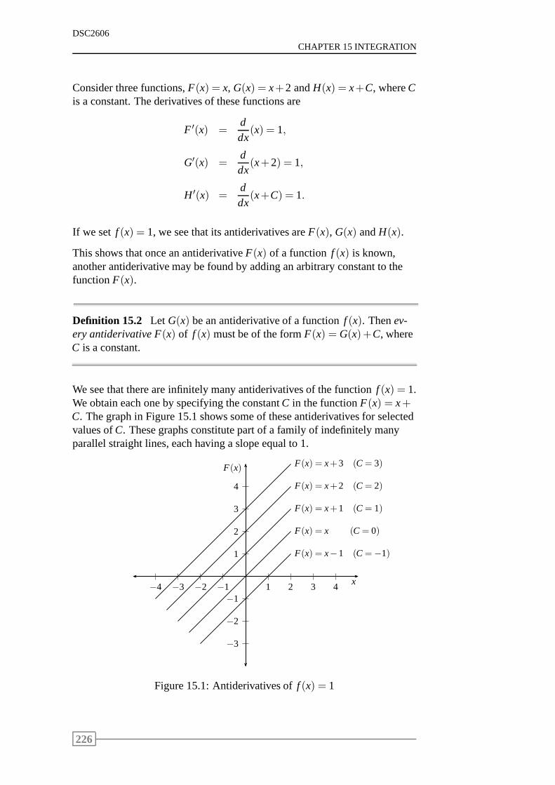
DSC2606
CHAPTER 15 INTEGRATION
Consider three functions,F(x) = x, G(x) = x+2 andH(x) = x+C, whereCis a constant. The derivatives of these functions are
F ′(x) =ddx
(x) = 1,
G′(x) =ddx
(x+2) = 1,
H ′(x) =ddx
(x+C) = 1.
If we set f (x) = 1, we see that its antiderivatives areF(x), G(x) andH(x).
This shows that once an antiderivativeF(x) of a function f (x) is known,another antiderivative may be found by adding an arbitrary constant to thefunctionF(x).
Definition 15.2 Let G(x) be an antiderivative of a functionf (x). Thenev-ery antiderivative F(x) of f (x) must be of the formF(x) = G(x)+C, whereC is a constant.
We see that there are infinitely many antiderivatives of the function f (x) = 1.We obtain each one by specifying the constantC in the functionF(x) = x+C. The graph in Figure 15.1 shows some of these antiderivatives for selectedvalues ofC. These graphs constitute part of a family of indefinitely manyparallel straight lines, each having a slope equal to 1.
1
2
3
4
−1
−2
−3
1 2 3 4−1−2−3−4
F(x)
x
F(x) = x−1 (C=−1)
F(x) = x (C= 0)
F(x) = x+1 (C= 1)
F(x) = x+2 (C= 2)
F(x) = x+3 (C= 3)
Figure 15.1: Antiderivatives off (x) = 1
226
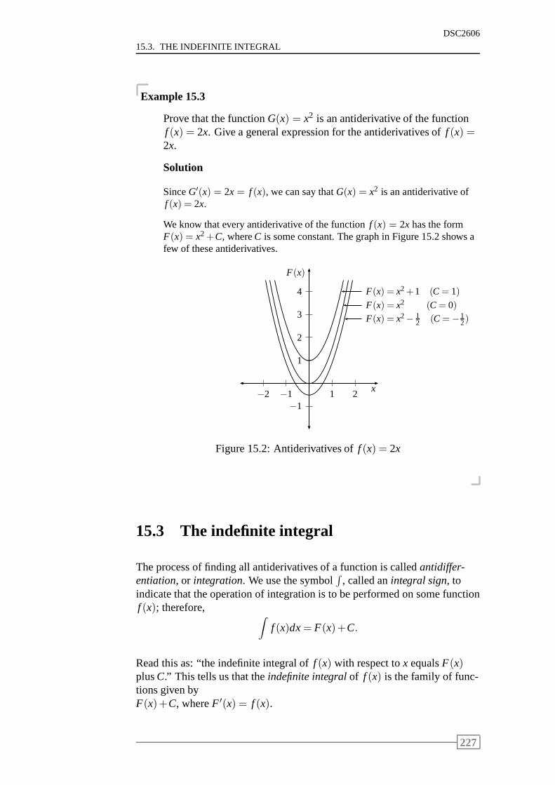
15.3. THE INDEFINITE INTEGRAL
DSC2606
Example 15.3
Prove that the functionG(x) = x2 is an antiderivative of the functionf (x) = 2x. Give a general expression for the antiderivatives off (x) =2x.
Solution
SinceG′(x) = 2x = f (x), we can say thatG(x) = x2 is an antiderivative off (x) = 2x.
We know that every antiderivative of the functionf (x) = 2x has the formF(x) = x2+C, whereC is some constant. The graph in Figure 15.2 shows afew of these antiderivatives.
1
2
3
4
−11 2−1−2
F(x)
x
F(x) = x2+1 (C= 1)
F(x) = x2 (C= 0)F(x) = x2− 1
2 (C=−12)
Figure 15.2: Antiderivatives off (x) = 2x
15.3 The indefinite integral
The process of finding all antiderivatives of a function is called antidiffer-entiation, or integration. We use the symbol
∫
, called anintegral sign, toindicate that the operation of integration is to be performed on some functionf (x); therefore,
∫
f (x)dx= F(x)+C.
Read this as: “the indefinite integral off (x) with respect tox equalsF(x)plusC.” This tells us that theindefinite integralof f (x) is the family of func-tions given byF(x)+C, whereF ′(x) = f (x).
227
DSC2606
CHAPTER 15 INTEGRATION
The functionf (x) to be integrated is called theintegrandand the constantC is called theconstant of integration. The expressiondx following the in-tegrandf (x) reminds us that the operation is performed with respect tox. If
the independent variable ist, we write∫
f (t)dt instead.
Using this notation, some previous results may be written as∫
1dx= x+C and∫
2xdx= x2+K,
whereC andK are arbitrary constants.
15.4 The basic rules of integration
In this section we give basic rules for finding the indefinite integral,F(x), ofa given functionf (x), and then verify them by showing thatF ′(x) = f (x).
Rule
∫
kdx= kx+C, k a constant.
Observe thatddx
(kx+C) = k.
Example 15.4
(a)∫
2dx= 2x+C.
(b)∫
π2dx= π2x+C.
RuleThe power rule is
∫
xndx=1
n+1xn+1+C, n 6=−1.
An antiderivative of a power function is another power function obtainedfrom the integrand by increasing its power by one and dividing the resultingexpression by the new power.
228
15.4. THE BASIC RULES OF INTEGRATION
DSC2606
Observe thatddx
(
1n+1
xn+1+C
)
=n+1n+1
xn = xn.
Example 15.5
(a)∫
x3dx=14
x4+C.
(b)∫
x32 dx=
152
x52 +C=
25
x52 +C.
(c)∫
1
x32
dx=∫
x−32dx=
1
−12
x−12 +C=
−2√x+C.
Rule
∫
c f(x)dx= c∫
f (x)dx, c a constant.
The indefinite integral of a constant multiple of a function is equal to theconstant multiple of the indefinite integral of the function.
Example 15.6
(a)
∫
2t3dt = 2∫
t3dt
= 2
(
14
t4+k
)
=12
t4+2k
=12
t4+C whereC= 2k.
NOTE:From now on we write the constant of integration asC, sinceany nonzero constant multiple of an arbitrary constant is anarbitraryconstant.
229
DSC2606
CHAPTER 15 INTEGRATION
(b)∫
(
−3x−2)dx = −3∫
x−2dx
= (−3)(−1)x−1+C
=3x+C.
RuleThe sum or difference rule
∫
[ f (x)+g(x)]dx=∫
f (x)dx+∫
g(x)dx
and∫
[ f (x)−g(x)]dx=∫
f (x)dx−∫
g(x)dx.
The indefinite integral of a sum (or difference) of two integrable functions isequal to the sum (or difference) of their integrals.
This result is easily extended to the case involving the sum (or difference) ofany finite number of functions.
230
15.4. THE BASIC RULES OF INTEGRATION
DSC2606
Example 15.7
∫
(
3x5+4x32 −2x−
12
)
dx =
∫
3x5dx+∫
4x32 dx−
∫
2x−12dx
= 3∫
x5dx+4∫
x32dx−2
∫
x−12 dx
= 3 · 16
x6+4 · 25
x52 −2 ·2x
12 +C
=12
x6+85
x52 −4√
x+C.
Rule
∫
exdx= ex+C.
The indefinite integral of the exponential function is equalto the functionitself plus the constant of integration.
Example 15.8
∫
(2ex)dx= 2∫
exdx= 2ex+C.
Rule
∫
x−1dx=∫
1x
dx= ln |x|+C.
The indefinite integral of x to the power−1, or one over x, is equal toln |x|plus the constant of integration.
NOTE:The power rule has an exception, namely that it is not applicable tox−1. Observe that
ddx
ln |x|= 1x.
(Rule 9.4 of differentiation)
231
DSC2606
CHAPTER 15 INTEGRATION
Example 15.9
∫
3x
dx= 3∫
1x
dx= 3ln|x|+C.
We now illustrate these rules of integration by means of someexamples.
Example 15.10
Find the the functionf (x) if it is known that f ′(x) = 3x2−4x+8 andf (1) = 9.
Solution
Integrating the functionf ′(x) we find
f (x) =∫
f ′(x)dx
=
∫
(
3x2−4x+8)
dx
= x3−2x2+8x+C.
Using the conditionf (1) = 9, we have
f (1) = 13−2(1)2+8(1)+C= 7+C= 9 ⇒C = 2.
Therefore, the required function is given byf (x) = x3−2x2+8x+2.
Example 15.11
The management of the Staedtler Office Company has determined thatthe daily marginal revenue function associated with producing andselling their battery-operated pencil sharpeners is givenby
R′(x) =−0,0006x+6,
wherex denotes the number of units produced and sold andR′(x) ismeasured in rand per unit.
Determine the revenue functionR(x) associated with producing andselling these pencil sharpeners.
232
15.5. INTEGRATION BY SUBSTITUTION
DSC2606
Solution
The revenue function is found by integrating the marginal revenue function
R(x) =∫
R′(x)dx
=∫
(−0,0006x+6)dx
= −0,0003x2+6x+C.
To determine the value of the constantC, observe that the revenue realisedby Staedtler is zero when the production and sales level is zero; that is,R(0) = 0. This condition implies that
R(0) =−0,0003(0)2+6(0)+C= 0 or C = 0.
The required revenue function is given byR(x) =−0,0003x2+6x.
15.5 Integration by substitution
In this section we introduce a method of integration called themethod ofsubstitution, which is related to the chain rule for differentiation. When usedin conjunction with the basic rules of integration, the method of substitutionis a powerful tool for integrating a large class of functions.
Consider the indefinite integral
∫
2(2x+4)5dx.
One way of evaluating this integral is to expand the expression (2x+4)5 andthen integrate the resulting integrand term by term.
Let us see if we can use an alternative approach to simplify this process. Wedo so by making a change in variable.
Let u= 2x+4 and since it is a function ofx, we writeu= 2x+4= g(x).
The derivative of this is
dudx
= 2 or g′(x) = 2.
We rewrite this as
dudx
= 2 ⇒ du= 2dx ⇒ du= g′(x)dx since g′(x) = 2.
233
DSC2606
CHAPTER 15 INTEGRATION
We now return to our original indefinite integral and substituteu = 2x+ 4anddu= 2dx into it. Then
∫
2(2x+4)5dx=∫
(2x+4)5(2dx) =∫
u5du.
Now the last integral involves a power function and is easilyevaluated usingthe power rule. Then
∫
u5du=16
u6+C.
Using this result and replacingu with 2x+4, we obtain
∫
2(2x+4)5dx=16(2x+4)6+C.
We can verify that the foregoing result is indeed correct by computing thefollowing by means of the chain rule:
ddx
[
16(2x+4)6
]
=16·6(2x+4)5(2) = 2(2x+4)5 ,
which is just the integrand.
Let us summarise the steps involved in integration by substitution:
Step 1: Let u = g(x), whereg(x) is part of the integrand, usually the “in-side function” of the composite functionf [g(x)].
Step 2: Calculateg′(x) and derivedu= g′(x)dx, (from g′(x) =dudx
).
Step 3: Use the substitutionu= g(x) anddu= g′(x)dx to convert theentireintegrand into one involving onlyu.
Step 4: Evaluate the resulting integral.
Step 5: Replaceu with g(x) to obtain the final solution as a function ofx.
Example 15.12
Evaluate∫
t2(t3+1)
32 dt.
Solution
Step 1: The integrand contains the composite function(
t3+1)
32 with “in-
side function”g(t) = t3+1. Letu= t3+1.
Step 2: Now g′(t) =dudt
= 3t2 ⇒ du= 3t2dt or t2dt =13
du.
234
15.5. INTEGRATION BY SUBSTITUTION
DSC2606
Step 3: Substituteu= t3+1 andt2dt = 13du, then
∫
t2(t3+1)
32 dt =
∫
u32
(
13
du
)
=13
∫
u32 du.
Step 4: Integrate:
13
∫
u32 du=
13· 25
u52 +C =
215
u52 +C.
Step 5: Replaceu with t3+1. Then
∫
t2(t3+1)
32 dt =
215
(
t3+1)
52 +C.
In the remaining examples, we drop the practice of labellingthe steps in-volved in evaluating each integral.
Example 15.13
Evaluate∫
a3a2+1
da.
Solution
Let u = 3a2+ 1. Thenduda
= 6a or du= 6adaor ada=16
du. Making the
appropriate substitutions we have
∫
a3a2+1
da =∫
1u· 16
du
=16
∫
1u
du
=16
ln |u|+C
=16
ln(
3a2+1)
+C (3a2+1> 0).
Example 15.14
Evaluate∫
(lnx)2
2xdx.
235
DSC2606
CHAPTER 15 INTEGRATION
Solution
Let u= lnx. Thendudx
=1x
or du=1x
dx.
Making the appropriate substitutions we have
∫
(lnx)2
2xdx =
∫
(lnx)2
2· 1x
dx
=∫
12
u2du
=16
u3+C
=16(lnx)3+C.
Example 15.15
A study prepared by the marketing department of the Universal Instru-ments Company forecasts that, after its new line of home computers isintroduced onto the market, sales will grow at the rate of
f (t) = 2000−1500e−0,05t for 0≤ t ≤ 60,
units per month.
(a) Find an expression that gives the total number of computers thatwill be soldt months after they become available on the market.
(b) How many computers will be sold in the first year they are onthemarket?
Solution
(a) LetN(t) denote the total number of computers that will be soldt monthsafter their introduction into the market. We have
N′(t) = 2000−1500e−0,05t.
Now
N(t) =∫
(
2000−1500e−0,05t)
dt
= 2000t−1500∫
e−0,05tdt.
236
15.6. THE AREA UNDER THE GRAPH OF A FUNCTION
DSC2606
Now letu=−0,05t, thendudt
=−0,05 anddu=−0,05dt. We have
∫
e−0,05tdt =∫
eu(
du−0,05
)
= − 10,05
∫
eudu
= − eu
0,05+C
= −e−0,05t
0,05+C.
Therefore,
N(t) = 2000t−1500
(
−e−0,05t
0,05+C
)
= 2000t+30000e−0,05t +C.
To determine the value ofC, note that the number of computers sold atthe end of month 0 is zero; soN(0) = 0. Now
N(0) = 30000e0+C= 30000+C ⇒C=−30000.
The required expression isN(t) = 2000t+30000e−0,05t−30000.
(b) The expressionN(12) will give the number of computers sold in thefirst year and
N(12) = 2000(12)+30000e−0,05(12)−30000
= 10464,35≈ 10464.
15.6 The area under the graph of a function
Suppose that a country’s annual rate of petrol consumption over a four-yearperiod is constant and is given by the function
f (t) = 1,2 for 0≤ t ≤ 4,
wheret is measured in years andf (t) in millions of barrels per year. Thecountry’s total petrol consumption (in million barrels) over the period oftime in question is
Rate of consumption× time lapsed= 1,2(4−0) = 4,8.
If we examine the graph in Figure 15.3, we see that this total is the area ofthe rectangular region bounded above by the graph off (t), below by the
237
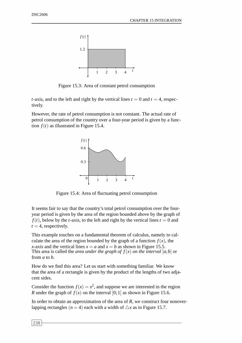
DSC2606
CHAPTER 15 INTEGRATION
1.2
1 2 3 4
f (t)
t
Figure 15.3: Area of constant petrol consumption
t-axis, and to the left and right by the vertical linest = 0 andt = 4, respec-tively.
However, the rate of petrol consumption is not constant. Theactual rate ofpetrol consumption of the country over a four-year period isgiven by a func-tion f (t) as illustrated in Figure 15.4.
0.3
0.6
1 2 3 40
f (t)
t
Figure 15.4: Area of fluctuating petrol consumption
It seems fair to say that the country’s total petrol consumption over the four-year period is given by the area of the region bounded above bythe graph off (t), below by thet-axis, to the left and right by the vertical linest = 0 andt = 4, respectively.
This example touches on a fundamental theorem of calculus, namely to cal-culate the area of the region bounded by the graph of a function f (x), thex-axis and the vertical linesx= a andx= b as shown in Figure 15.5.This area is called thearea under the graph of f(x) on the interval[a;b] orfrom a to b.
How do we find this area? Let us start with something familiar.We knowthat the area of a rectangle is given by the product of the lengths of two adja-cent sides.
Consider the functionf (x) = x2, and suppose we are interested in the regionR under the graph off (x) on the interval[0;1] as shown in Figure 15.6.
In order to obtain an approximation of the area ofR, we construct four nonover-lapping rectangles(n= 4) each with a width of△x as in Figure 15.7.
238
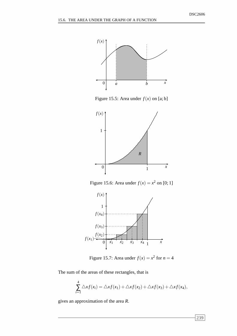
15.6. THE AREA UNDER THE GRAPH OF A FUNCTION
DSC2606
a b0
f (x)
x
Figure 15.5: Area underf (x) on [a; b]
1
10
f (x)
x
R
Figure 15.6: Area underf (x) = x2 on [0; 1]
1
10
f (x)
xx1f (x1)
x2
f (x2)
x3
f (x3)
x4
f (x4)
Figure 15.7: Area underf (x) = x2 for n= 4
The sum of the areas of these rectangles, that is
4
∑i=1△x f(xi) =△x f(x1)+△x f(x2)+△x f(x3)+△x f(x4),
gives an approximation of the areaR.
239
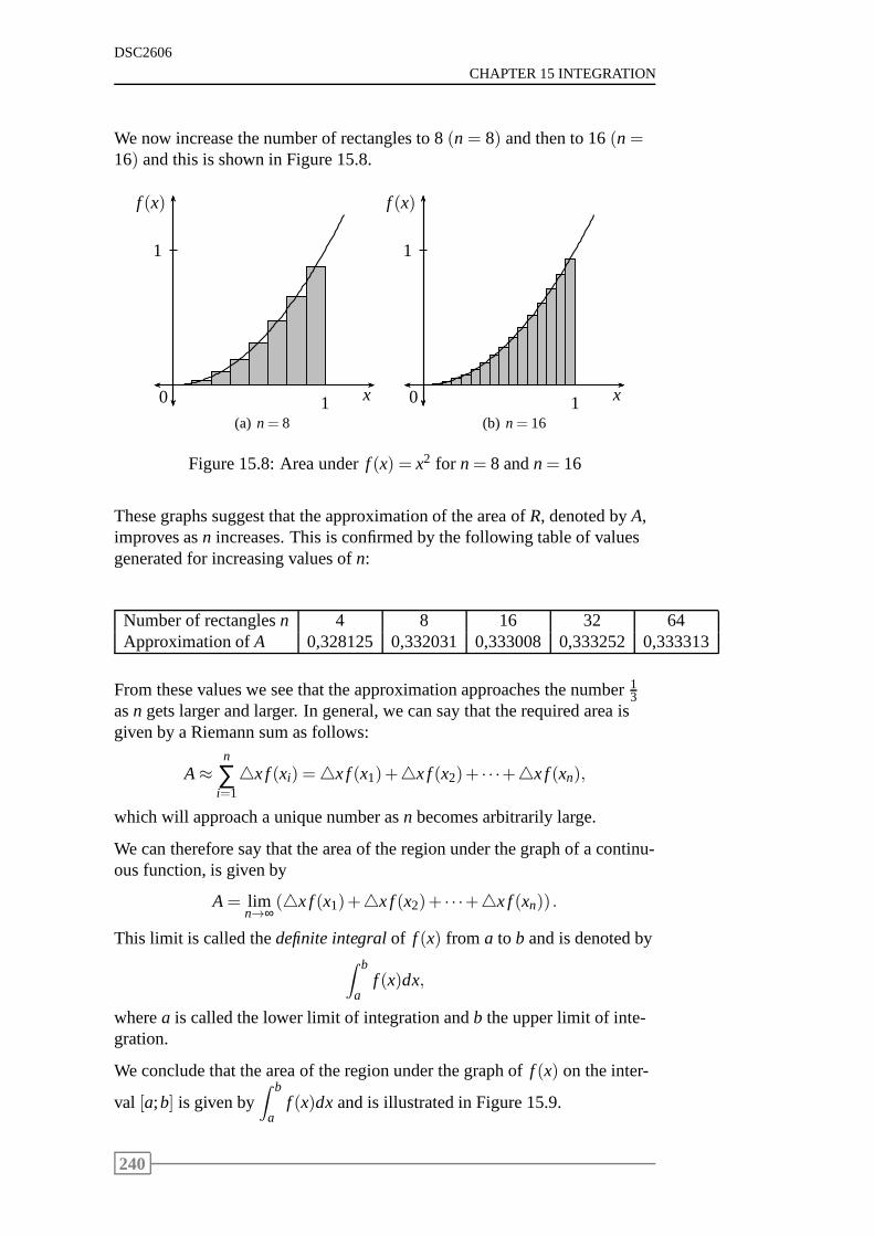
DSC2606
CHAPTER 15 INTEGRATION
We now increase the number of rectangles to 8(n = 8) and then to 16(n=16) and this is shown in Figure 15.8.
1
10
f (x)
x
(a) n= 8
1
10
f (x)
x
(b) n= 16
Figure 15.8: Area underf (x) = x2 for n= 8 andn= 16
These graphs suggest that the approximation of the area ofR, denoted byA,improves asn increases. This is confirmed by the following table of valuesgenerated for increasing values ofn:
Number of rectanglesn 4 8 16 32 64Approximation ofA 0,328125 0,332031 0,333008 0,333252 0,333313
From these values we see that the approximation approaches the number13asn gets larger and larger. In general, we can say that the required area isgiven by a Riemann sum as follows:
A≈n
∑i=1△x f(xi) =△x f(x1)+△x f(x2)+ · · ·+△x f(xn),
which will approach a unique number asn becomes arbitrarily large.
We can therefore say that the area of the region under the graph of a continu-ous function, is given by
A= limn→∞
(△x f(x1)+△x f(x2)+ · · ·+△x f(xn)) .
This limit is called thedefinite integralof f (x) from a to b and is denoted by∫ b
af (x)dx,
wherea is called the lower limit of integration andb the upper limit of inte-gration.
We conclude that the area of the region under the graph off (x) on the inter-
val [a;b] is given by∫ b
af (x)dx and is illustrated in Figure 15.9.
240
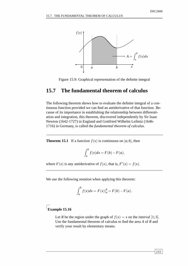
15.7. THE FUNDAMENTAL THEOREM OF CALCULUS
DSC2606
a b0
f (x)
x
A=∫ b
af (x)dx
Figure 15.9: Graphical representation of the definite integral
15.7 The fundamental theorem of calculus
The following theorem shows how to evaluate the definite integral of a con-tinuous function provided we can find an antiderivative of that function. Be-cause of its importance in establishing the relationship between differenti-ation and integration, this theorem, discovered independently by Sir IsaacNewton (1642-1727) in England and Gottfried Wilhelm Leibniz (1646-1716) in Germany, is called thefundamental theorem of calculus.
Theorem 15.1 If a function f (x) is continuous on[a;b], then
∫ b
af (x)dx= F(b)−F(a),
whereF(x) is any antiderivative off (x), that is,F ′(x) = f (x).
We use the following notation when applying this theorem:
∫ b
af (x)dx= F(x)|ba = F(b)−F(a).
Example 15.16
Let R be the region under the graph off (x) = x on the interval[1;3].Use the fundamental theorem of calculus to find the areaA of Randverify your result by elementary means.
241
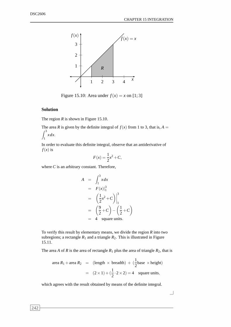
DSC2606
CHAPTER 15 INTEGRATION
1
2
3
1 2 3 4
f (x)
x
f (x) = x
R
Figure 15.10: Area underf (x) = x on [1; 3]
Solution
The regionR is shown in Figure 15.10.
The areaR is given by the definite integral off (x) from 1 to 3, that is,A =∫ 3
1xdx.
In order to evaluate this definite integral, observe that an antiderivative off (x) is
F(x) =12
x2+C,
whereC is an arbitrary constant. Therefore,
A =∫ 3
1xdx
= F(x)|31
=
(
12
x2+C
)∣
∣
∣
∣
3
1
=
(
92+C
)
−(
12+C
)
= 4 square units.
To verify this result by elementary means, we divide the regionR into twosubregions; a rectangleR1 and a triangleR2. This is illustrated in Figure15.11.
The areaA of R is the area of rectangleR1 plus the area of triangleR2, that is
areaR1+areaR2 = (length× breadth) + (12
base×height)
= (2×1)+(12·2×2) = 4 square units,
which agrees with the result obtained by means of the definiteintegral.
242
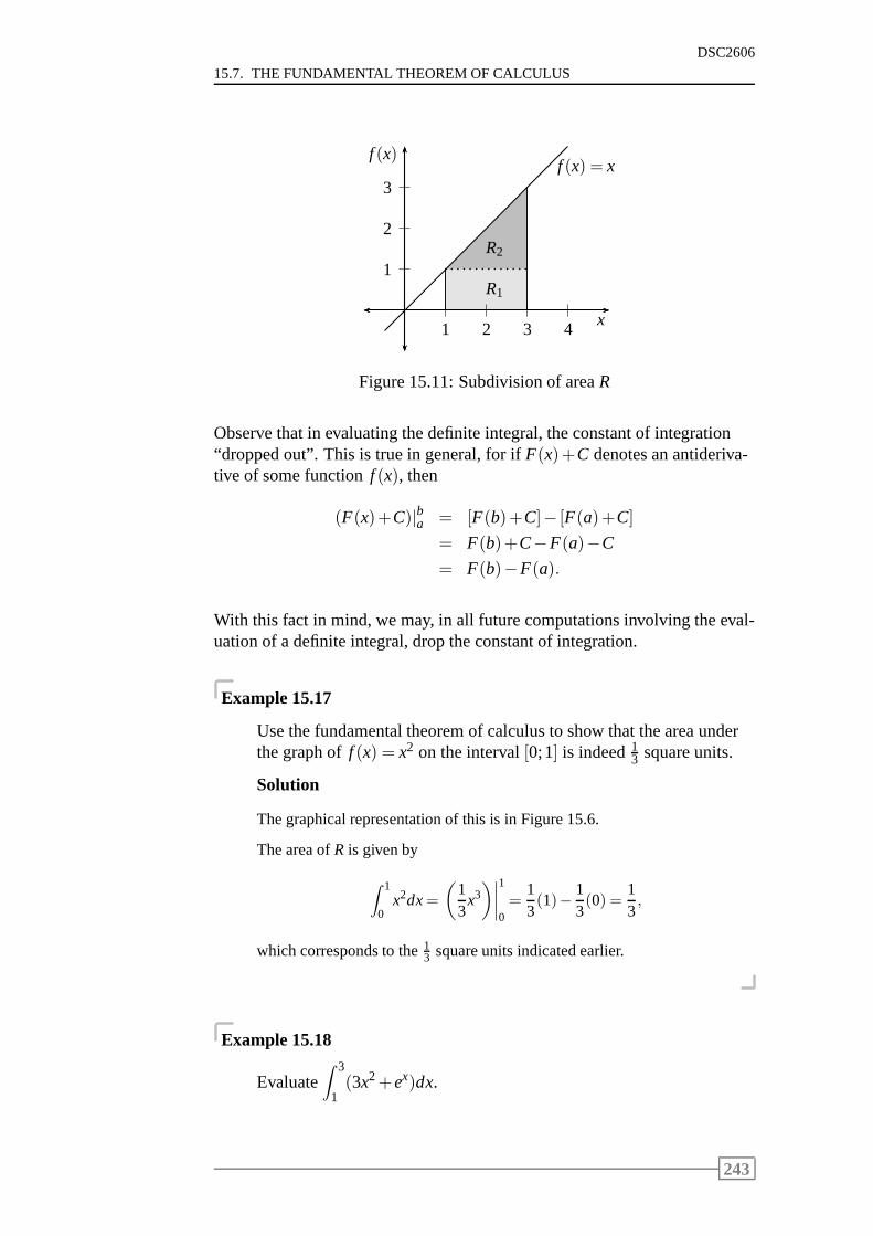
15.7. THE FUNDAMENTAL THEOREM OF CALCULUS
DSC2606
1
2
3
1 2 3 4
f (x)
x
f (x) = x
R1
R2
Figure 15.11: Subdivision of areaR
Observe that in evaluating the definite integral, the constant of integration“dropped out”. This is true in general, for ifF(x)+C denotes an antideriva-tive of some functionf (x), then
(F(x)+C)|ba = [F(b)+C]− [F(a)+C]
= F(b)+C−F(a)−C
= F(b)−F(a).
With this fact in mind, we may, in all future computations involving the eval-uation of a definite integral, drop the constant of integration.
Example 15.17
Use the fundamental theorem of calculus to show that the areaunderthe graph off (x) = x2 on the interval[0;1] is indeed1
3 square units.
Solution
The graphical representation of this is in Figure 15.6.
The area ofR is given by
∫ 1
0x2dx=
(
13
x3)∣
∣
∣
∣
1
0=
13(1)− 1
3(0) =
13,
which corresponds to the13 square units indicated earlier.
Example 15.18
Evaluate∫ 3
1(3x2+ex)dx.
243
DSC2606
CHAPTER 15 INTEGRATION
Solution
The definite integral is∫ 3
1(3x2+ex)dx =
∫ 3
13x2dx+
∫ 3
1exdx
= x3∣
∣
31+ ex|31
=(
33−11)+(
e3−e1)
= 26+e3−e1 = 43,37.
Example 15.19
The management of Staedtler Office Equipment has determinedthatthe daily marginal cost function associated with producingbattery-operated pencil sharpeners is given by
C′(x) = 0,000006x2−0,006x+4,
whereC′(x) is measured in rand per unit andx denotes the number ofunits produced. Management has also determined that the daily fixedcost incurred in producing pencil sharpeners is R100.
(a) What is Staedtler’s daily total cost if 500 pencil sharpeners areproduced?
(b) What is the additional daily cost incurred if the production ofpencil sharpeners increases from 200 to 400 units?
Solution
(a) The daily total cost function is
C(x) =
∫
C′(x)dx
=∫
(0,000006x2−0,006x+4)dx
=0,000006
3x3− 0,006
2x2+4x+k
= 0,000002x3−0,003x2+4x+k.
We must determine the value of the constant of integrationk. The dailyfixed cost is R100. This means that a cost of R100 is incurred even ifno pencil sharpeners are produced; soC(0) = 100. Now substitutingthis intoC(x), we have
C(0) = 0,000002(0)3−0,003(0)2+4(0)+k= 100 ⇒ k= 100.
The daily total cost function is
C(x) = 0,000002x3−0,003x2+4x+100.
244
15.8. THE METHOD OF SUBSTITUTION FOR DEFINITE INTEGRALS
DSC2606
We must determine the daily total cost if 500 pencil sharpeners areproduced and this is
C(500)=0,000002(500)3−0,003(500)2+4(500)+100=1600 (rand).
An alternative method of calculating the daily total cost may be usedand is as follows:
We are required to calculateC(500). Let us calculateC(500)−C(0),which is the change in the total cost functionC(x) over the interval[0;500].
Using the fundamental theorem of calculus, we find
C(500)−C(0) =∫ 500
0C′(x)dx
=(
0,000002x3−0,003x2+4x)∣
∣
5000
= 1500−0= 1500.
From this it follows that
C(500) = 1500+C(0)
= 1500+100= 1600 (rand),
which is the same result as before. Therefore, the daily total cost if 500pencil sharpeners are produced is R1600.
(b) The additional daily cost incurred if the production of pencil sharpen-ers is increased from 200 to 400 units is given by
C(400)−C(200) =∫ 400
200C′(x)dx
=(
0,000002x3−0,003x2+4x)∣
∣
400200
= 1248−696= 552 (rand).
15.8 The method of substitution for definite inte-grals
Suppose we have to evaluate the following definite integral:
∫ 4
0x√
9+x2dx.
We can do this by using one of two methods.
Method 1
We first find the corresponding indefinite integralI =∫
x√
9+x2dx.
245
DSC2606
CHAPTER 15 INTEGRATION
Let u= 9+x2. Thendudx
= 2x or du= 2xdxor xdx=12
du. Now
I =∫
x√
9+x2dx =∫
(9+x2)12(xdx)
=∫
u12 · 1
2du
=12
∫
u12 du
=12· 23
u32 +C
=13(9+x2)
32 +C.
Using this result, we now evaluate the given definite integral. Then
∫ 4
0x√
9+x2dx =13(9+x2)
32
∣
∣
∣
∣
4
0
=13
[
(9+16)32 −9
32
]
=13(125−27)
=983
= 3223.
Method 2
As before, we make the substitutionu = 9+ x2, so thatdudx
= 2x or du=
2xdxor xdx=12
du. Now observe that the given definite integral is eval-
uatedwith respect to x, with the range of integration given by the interval[0;4]. If we perform the integration with respect tou via the substitutionu = 9+ x2, then we must adjust the range of integration to reflect the factthat the integration is being performed with respect to the new variableu.We now determine the proper range of integration as follows:
Whenx = 0, u = 9+ 02 = 9, the required lower limit of integration withrespect tou, and whenx = 4, u = 9+42 = 25, the required upper limit ofintegration with respect tou.
The range of integration when the integration is performed with respect tou
246
15.8. THE METHOD OF SUBSTITUTION FOR DEFINITE INTEGRALS
DSC2606
is given by the interval[9;25]. Therefore, we have
∫ 4
0x√
9+x2dx =
∫ 4
0(9+x2)
12 (xdx)
=∫ 25
9u
12
(
12
du
)
=12
∫ 25
9u
12du
=13
u32
∣
∣
∣
∣
25
9
=13(25
32 −9
32)
=13(125−27)
=983
= 3223,
which agrees with the result obtained using Method 1.
Example 15.20
Evaluate∫ 2
0xe2x2
dx.
Solution
Let u= 2x2. Thendudx
= 4x or du= 4xdxor xdx=14
du.
If x= 0, thenu= 0 and ifx= 2, thenu= 8. Therefore,
∫ 2
0xe2x2
dx =
∫ 2
0e2x2
(xdx)
=∫ 8
0eu(
14
du
)
=14
∫ 8
0eudu
=14
eu
∣
∣
∣
∣
8
0
=14(e8−e0)
≈ 745.
247

DSC2606
CHAPTER 15 INTEGRATION
15.9 Consumers’ and producers’ surplus
15.9.1 Consumers’ surplus
Supposep = D(x) is the demand function that relates the unit pricep of acommodity to the quantityx demanded of it. And suppose that a fixed unitmarket price ¯p has been established for the commodity and that, correspond-ing to this unit price, the quantity demanded is ¯x units.
Then those customers who would be willing to pay a unit price higher thanp̄ for the commodity would in effect experience a saving. This differencebetween what the consumerswould be willing to payfor x̄ units of the com-modity and what theyactually payis called theconsumers’ surplus.
The shaded area on the graph in Figure 15.12 represents the consumers’ sur-plus.
D(x)
xx̄
p̄
Figure 15.12: Consumers’ surplus
The consumers’ surplus is calculated by subtracting the area of the rectan-gle, p̄× x̄, from the total area under the graph ofD(x) on the interval[0;x̄].
Definition 15.3 Theconsumers’ surplusis given by
CS=∫ x̄
0D(x)dx− p̄ · x̄,
whereD(x) is the demand function, ¯p is the fixed unit market price, ¯x is thequantity sold andCSis in rand.
15.9.2 Producers’ surplus
Supposep = S(x) is the supply function that relates the unit pricep of acommodity to the quantityx that the supplier will make available in the mar-
248
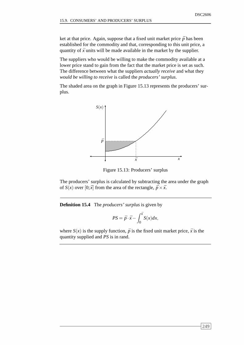
15.9. CONSUMERS’ AND PRODUCERS’ SURPLUS
DSC2606
ket at that price. Again, suppose that a fixed unit market price p̄ has beenestablished for the commodity and that, corresponding to this unit price, aquantity ofx̄ units will be made available in the market by the supplier.
The suppliers who would be willing to make the commodity available at alower price stand to gain from the fact that the market price is set as such.The difference between what the suppliersactually receiveand what theywould be willing to receiveis called theproducers’ surplus.
The shaded area on the graph in Figure 15.13 represents the producers’ sur-plus.
S(x)
xx̄
p̄
Figure 15.13: Producers’ surplus
The producers’ surplus is calculated by subtracting the area under the graphof S(x) over[0;x̄] from the area of the rectangle, ¯p× x̄.
Definition 15.4 Theproducers’ surplusis given by
PS= p̄ · x̄−∫ x̄
0S(x)dx,
whereS(x) is the supply function, ¯p is the fixed unit market price, ¯x is thequantity supplied andPSis in rand.
249
DSC2606
CHAPTER 15 INTEGRATION
Example 15.21
The demand function for a certain make of compact disk is given by
p= D(x) =−0,001x2+250,
wherep is the unit price in rand andx is the quantity demanded inunits of a thousand. The supply function for these disks is given by
p= S(x) = 0,0006x2+0,02x+100,
wherep is the unit price in rand andx is the number of disks that thesupplier will put on the market in units of a thousand.
Determine the consumers’ surplus and producers’ surplus ifthe mar-ket price of a disk is set at the equilibrium price.
Solution
The equilibrium price is the unit price of the commodity whenmarket equi-librium occurs. We determine the equilibrium price by determining the pointof intersection of the demand function and the supply function. We find thispoint by solving the demand and supply functions simultaneously, that is
p=−0,001x2+250
andp= 0,0006x2+0,02x+100.
Therefore, we have
0,0006x2+0,02x+100 = −0,001x2+250
0,0016x2+0,02x−150 = 0
16x2+200x−1500000 = 0
2x2+25x−187500 = 0
(2x+625)(x−300) = 0
⇒ x=−6252 or x= 300.
A negative quantity is impossible; therefore, we are left with the solutionx= 300. The correspondingp-value is
p=−0,001(300)2+250= 160.
The equilibrium point is(300;160); that is, the equilibrium quantity is 300000and the equilibrium price is R160.
Setting the market price at R160 per unit, we find that the consumers’ sur-plus is given by
CS =∫ x̄
0D(x)dx− p̄· x̄
=∫ 300
0(−0,001x2+250)dx− (160)(300)
=
(
− 13000
x3+250x
)∣
∣
∣
∣
300
0−48000
= 66000−48000
= 18000.
250
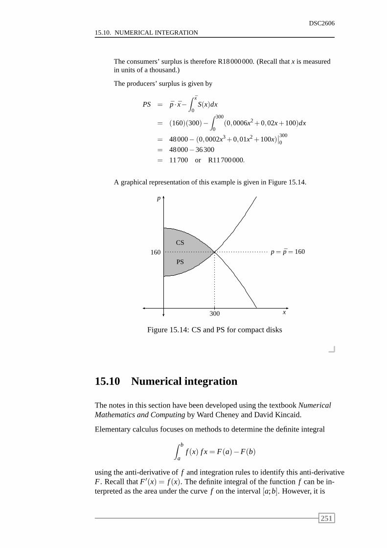
15.10. NUMERICAL INTEGRATION
DSC2606
The consumers’ surplus is therefore R18000000. (Recall that x is measuredin units of a thousand.)
The producers’ surplus is given by
PS = p̄· x̄−∫ x̄
0S(x)dx
= (160)(300)−∫ 300
0(0,0006x2+0,02x+100)dx
= 48000− (0,0002x3+0,01x2+100x)∣
∣
3000
= 48000−36300
= 11700 or R11700000.
A graphical representation of this example is given in Figure 15.14.
p
x
p= p̄= 160
300
160
CS
PS
Figure 15.14: CS and PS for compact disks
15.10 Numerical integration
The notes in this section have been developed using the textbookNumericalMathematics and Computingby Ward Cheney and David Kincaid.
Elementary calculus focuses on methods to determine the definite integral
∫ b
af (x) f x= F(a)−F(b)
using the anti-derivative off and integration rules to identify this anti-derivativeF. Recall thatF ′(x) = f (x). The definite integral of the functionf can be in-terpreted as the area under the curvef on the interval[a;b]. However, it is
251
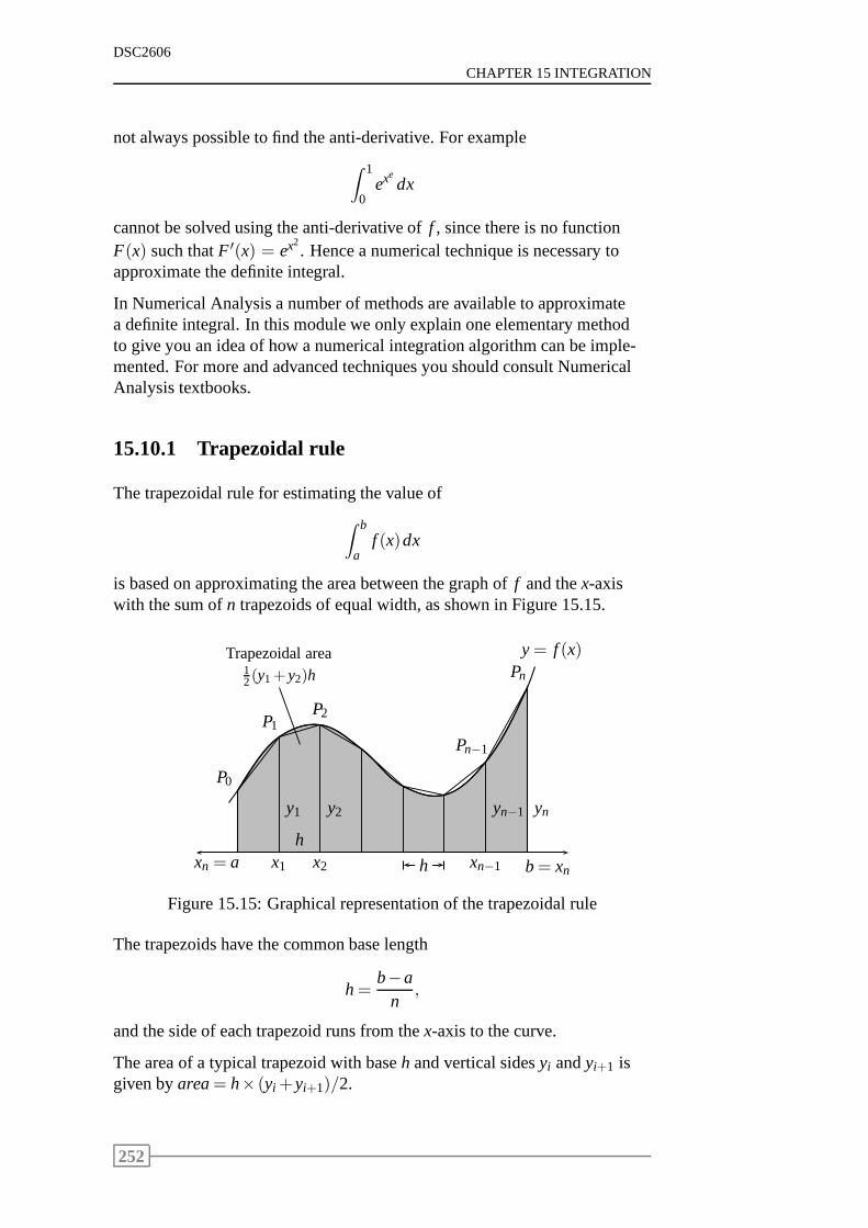
DSC2606
CHAPTER 15 INTEGRATION
not always possible to find the anti-derivative. For example
∫ 1
0exe
dx
cannot be solved using the anti-derivative off , since there is no functionF(x) such thatF ′(x) = ex2
. Hence a numerical technique is necessary toapproximate the definite integral.
In Numerical Analysis a number of methods are available to approximatea definite integral. In this module we only explain one elementary methodto give you an idea of how a numerical integration algorithm can be imple-mented. For more and advanced techniques you should consultNumericalAnalysis textbooks.
15.10.1 Trapezoidal rule
The trapezoidal rule for estimating the value of
∫ b
af (x)dx
is based on approximating the area between the graph off and thex-axiswith the sum ofn trapezoids of equal width, as shown in Figure 15.15.
h
y= f (x)
P0
P1P2
Pn−1
Pn
y1 y2 yn−1 yn
x1 x2 xn−1 b= xnxn = ah
Trapezoidal area12(y1+y2)h
Figure 15.15: Graphical representation of the trapezoidalrule
The trapezoids have the common base length
h=b−a
n,
and the side of each trapezoid runs from thex-axis to the curve.
The area of a typical trapezoid with baseh and vertical sidesyi andyi+1 isgiven byarea= h× (yi +yi+1)/2.
252
15.10. NUMERICAL INTEGRATION
DSC2606
RuleTrapezoidal Rule
Divide the interval[a;b] into n subintervals[xi ;xi+1] of width h= (b−a)/n,with x0 = a andxn = b. Hencexi = a+ ih, for i = 0;1;. . . ;n.
On each subinterval[xi ;xi+1], the area under the curvef (x) can be approxi-mated by the area of the trapezoid
T(i) =h2(yi +yi+1) =
h2[ f (xi)+ f (xi+1)].
The total area underneath the curve can be approximated by the sum of theareas of then trapezoids. Hence:
∫ b
af (x)dx ≈ T(1)+T(2)+ . . .T(n)
=h2(y0+y1)+
h2(y1+y2)+ . . .
h2(yn+yn−1)
=h2+h(y1+y2+ . . .yn−1)+
h2
yn
=h2[ f (x0)+ f (xn)]+h
n−1
∑i=1
f (xi)
=h2[ f (a)+ f (b)]+h
n−1
∑i=1
f (xi)
253
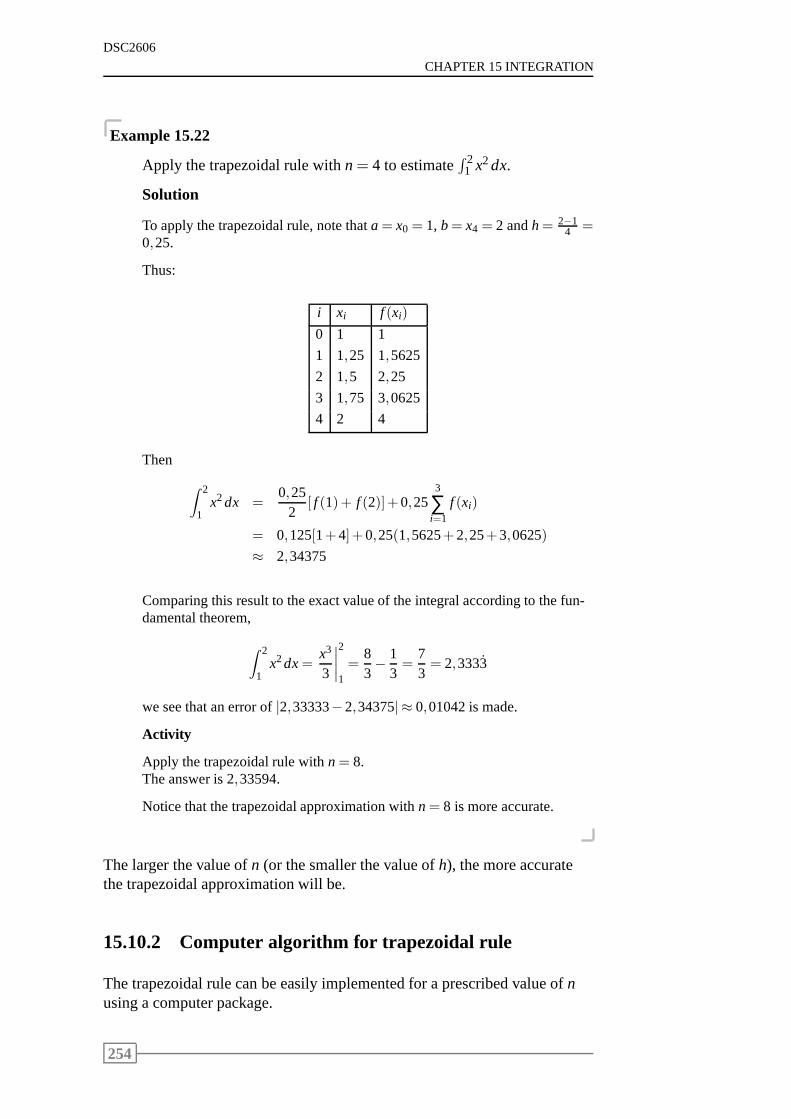
DSC2606
CHAPTER 15 INTEGRATION
Example 15.22
Apply the trapezoidal rule withn= 4 to estimate∫ 2
1 x2dx.
Solution
To apply the trapezoidal rule, note thata= x0 = 1, b= x4 = 2 andh= 2−14 =
0,25.
Thus:
i xi f (xi)
0 1 1
1 1,25 1,5625
2 1,5 2,25
3 1,75 3,0625
4 2 4
Then
∫ 2
1x2dx =
0,252
[ f (1)+ f (2)]+0,253
∑i=1
f (xi)
= 0,125[1+4]+0,25(1,5625+2,25+3,0625)
≈ 2,34375
Comparing this result to the exact value of the integral according to the fun-damental theorem,
∫ 2
1x2dx=
x3
3
∣
∣
∣
∣
2
1=
83− 1
3=
73= 2,3333̇
we see that an error of|2,33333−2,34375| ≈ 0,01042 is made.
Activity
Apply the trapezoidal rule withn= 8.The answer is 2,33594.
Notice that the trapezoidal approximation withn= 8 is more accurate.
The larger the value ofn (or the smaller the value ofh), the more accuratethe trapezoidal approximation will be.
15.10.2 Computer algorithm for trapezoidal rule
The trapezoidal rule can be easily implemented for a prescribed value ofnusing a computer package.
254
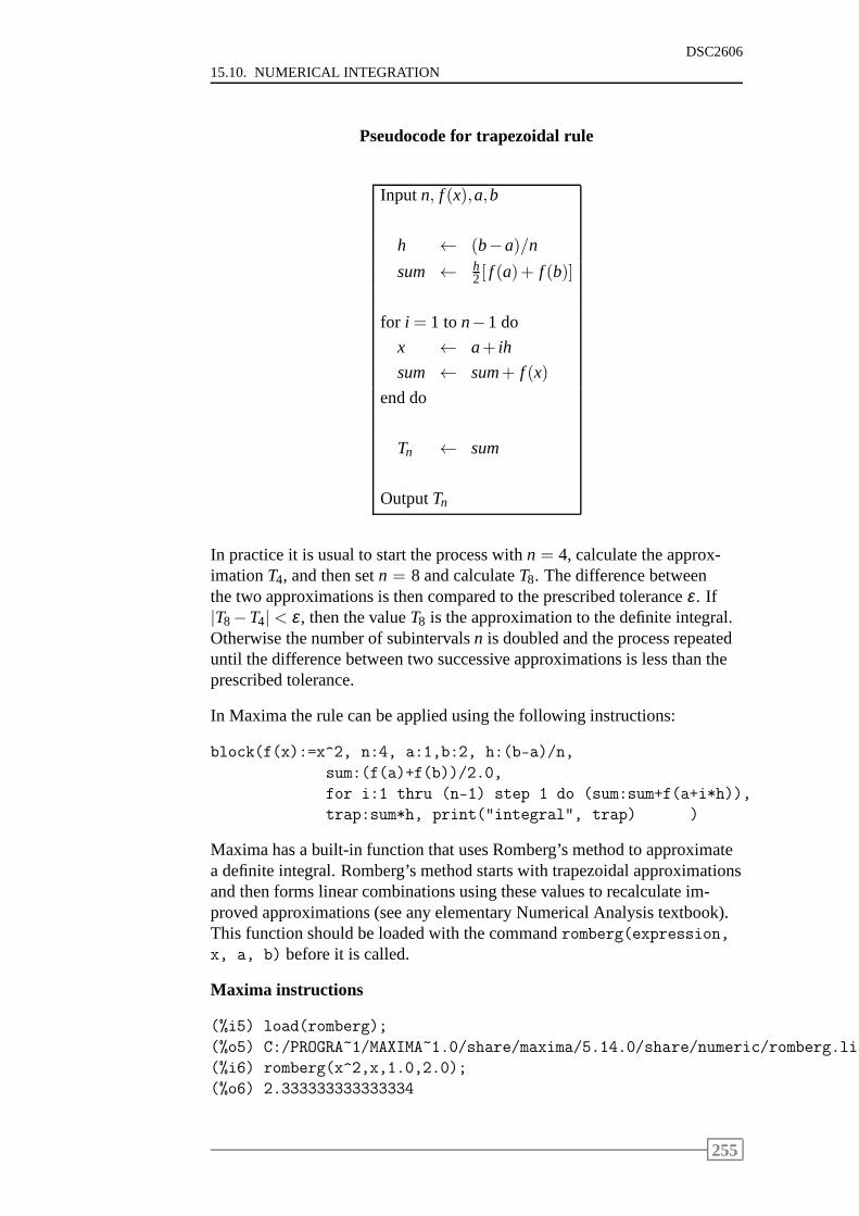
15.10. NUMERICAL INTEGRATION
DSC2606
Pseudocode for trapezoidal rule
Inputn, f (x),a,b
h ← (b−a)/n
sum ← h2[ f (a)+ f (b)]
for i = 1 ton−1 do
x ← a+ ih
sum ← sum+ f (x)
end do
Tn ← sum
OutputTn
In practice it is usual to start the process withn = 4, calculate the approx-imationT4, and then setn = 8 and calculateT8. The difference betweenthe two approximations is then compared to the prescribed toleranceε. If|T8−T4| < ε, then the valueT8 is the approximation to the definite integral.Otherwise the number of subintervalsn is doubled and the process repeateduntil the difference between two successive approximations is less than theprescribed tolerance.
In Maxima the rule can be applied using the following instructions:
block(f(x):=x^2, n:4, a:1,b:2, h:(b-a)/n,
sum:(f(a)+f(b))/2.0,
for i:1 thru (n-1) step 1 do (sum:sum+f(a+i*h)),
trap:sum*h, print("integral", trap) )
Maxima has a built-in function that uses Romberg’s method toapproximatea definite integral. Romberg’s method starts with trapezoidal approximationsand then forms linear combinations using these values to recalculate im-proved approximations (see any elementary Numerical Analysis textbook).This function should be loaded with the commandromberg(expression,
x, a, b) before it is called.
Maxima instructions
(%i5) load(romberg);
(%o5) C:/PROGRA~1/MAXIMA~1.0/share/maxima/5.14.0/share/numeric/romberg.lisp
(%i6) romberg(x^2,x,1.0,2.0);
(%o6) 2.333333333333334
255
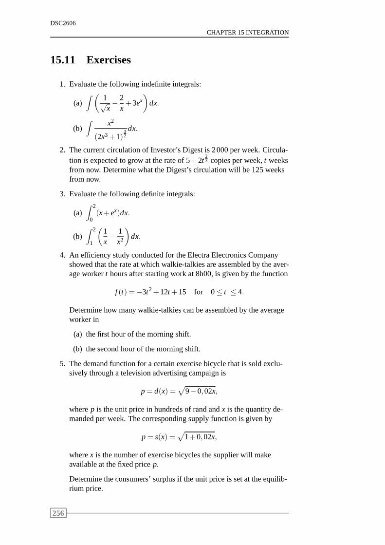
DSC2606
CHAPTER 15 INTEGRATION
15.11 Exercises
1. Evaluate the following indefinite integrals:
(a)∫
(
1√x− 2
x+3ex
)
dx.
(b)∫
x2
(2x3+1)32
dx.
2. The current circulation of Investor’s Digest is 2000 per week. Circula-tion is expected to grow at the rate of 5+2t
23 copies per week,t weeks
from now. Determine what the Digest’s circulation will be 125 weeksfrom now.
3. Evaluate the following definite integrals:
(a)∫ 2
0(x+ex)dx.
(b)∫ 2
1
(
1x− 1
x2
)
dx.
4. An efficiency study conducted for the Electra ElectronicsCompanyshowed that the rate at which walkie-talkies are assembled by the aver-age workert hours after starting work at 8h00, is given by the function
f (t) =−3t2+12t+15 for 0≤ t ≤ 4.
Determine how many walkie-talkies can be assembled by the averageworker in
(a) the first hour of the morning shift.
(b) the second hour of the morning shift.
5. The demand function for a certain exercise bicycle that issold exclu-sively through a television advertising campaign is
p= d(x) =√
9−0,02x,
wherep is the unit price in hundreds of rand andx is the quantity de-manded per week. The corresponding supply function is givenby
p= s(x) =√
1+0,02x,
wherex is the number of exercise bicycles the supplier will makeavailable at the fixed pricep.
Determine the consumers’ surplus if the unit price is set at the equilib-rium price.
256
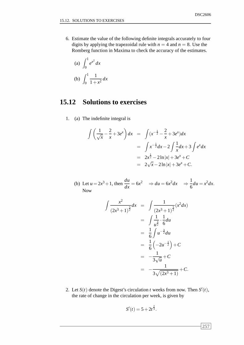
15.12. SOLUTIONS TO EXERCISES
DSC2606
6. Estimate the value of the following definite integrals accurately to fourdigits by applying the trapezoidal rule withn = 4 andn = 8. Use theRomberg function in Maxima to check the accuracy of the estimates.
(a)∫ 1
0ex2
dx
(b)∫ 1
0
11+x2 dx
15.12 Solutions to exercises
1. (a) The indefinite integral is
∫
(
1√x− 2
x+3ex
)
dx =∫
(x−12 − 2
x+3ex)dx
=∫
x−12 dx−2
∫
1x
dx+3∫
exdx
= 2x12 −2ln|x|+3ex+C
= 2√
x−2ln|x|+3ex+C.
(b) Letu=2x3+1, thendudx
= 6x2 ⇒ du= 6x2dx ⇒ 16
du= x2dx.
Now
∫
x2
(2x3+1)32
dx =
∫
1
(2x3+1)32
(x2dx)
=∫
1
u32
· 16
du
=16
∫
u−32du
=16
(
−2u−12
)
+C
= − 13√
u+C
= − 1
3√
(2x3+1)+C.
2. LetS(t) denote the Digest’s circulationt weeks from now. ThenS′(t),the rate of change in the circulation per week, is given by
S′(t) = 5+2t23 .
257
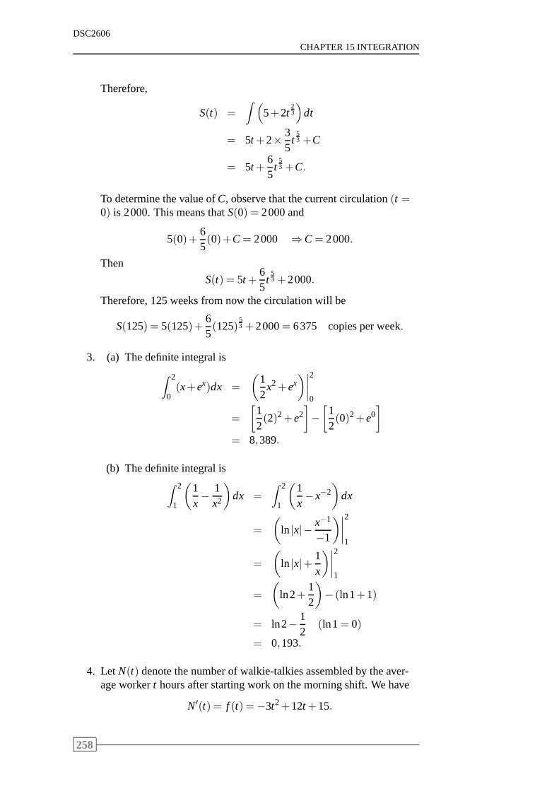
DSC2606
CHAPTER 15 INTEGRATION
Therefore,
S(t) =
∫
(
5+2t23
)
dt
= 5t+2× 35
t53 +C
= 5t+65
t53 +C.
To determine the value ofC, observe that the current circulation(t =0) is 2000. This means thatS(0) = 2000 and
5(0)+65(0)+C= 2000 ⇒C= 2000.
Then
S(t) = 5t +65
t53 +2000.
Therefore, 125 weeks from now the circulation will be
S(125) = 5(125)+65(125)
53 +2000= 6375 copies per week.
3. (a) The definite integral is
∫ 2
0(x+ex)dx =
(
12
x2+ex)∣
∣
∣
∣
2
0
=
[
12(2)2+e2
]
−[
12(0)2+e0
]
= 8,389.
(b) The definite integral is∫ 2
1
(
1x− 1
x2
)
dx =
∫ 2
1
(
1x−x−2
)
dx
=
(
ln |x|− x−1
−1
)∣
∣
∣
∣
2
1
=
(
ln |x|+ 1x
)∣
∣
∣
∣
2
1
=
(
ln2+12
)
− (ln1+1)
= ln2− 12
(ln1= 0)
= 0,193.
4. LetN(t) denote the number of walkie-talkies assembled by the aver-age workert hours after starting work on the morning shift. We have
N′(t) = f (t) =−3t2+12t +15.
258
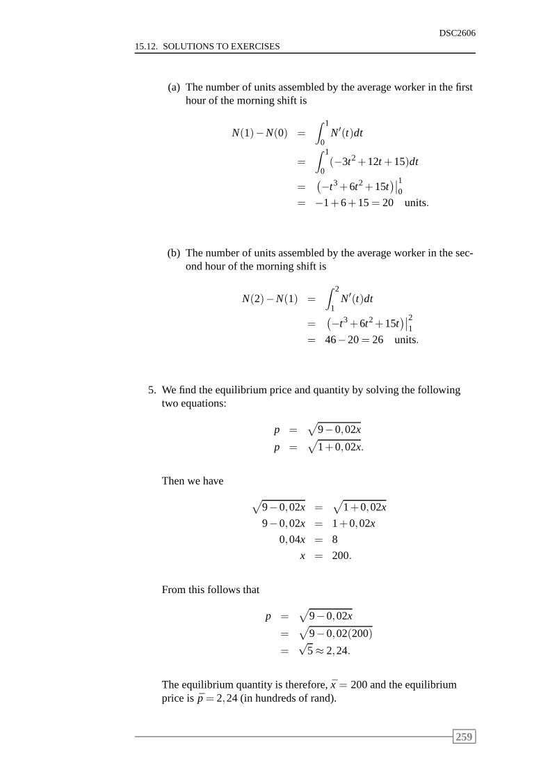
15.12. SOLUTIONS TO EXERCISES
DSC2606
(a) The number of units assembled by the average worker in thefirsthour of the morning shift is
N(1)−N(0) =∫ 1
0N′(t)dt
=
∫ 1
0(−3t2+12t +15)dt
=(
−t3+6t2+15t)∣
∣
10
= −1+6+15= 20 units.
(b) The number of units assembled by the average worker in thesec-ond hour of the morning shift is
N(2)−N(1) =
∫ 2
1N′(t)dt
=(
−t3+6t2+15t)∣
∣
21
= 46−20= 26 units.
5. We find the equilibrium price and quantity by solving the followingtwo equations:
p =√
9−0,02x
p =√
1+0,02x.
Then we have
√
9−0,02x =√
1+0,02x
9−0,02x = 1+0,02x
0,04x = 8
x = 200.
From this follows that
p =√
9−0,02x
=√
9−0,02(200)
=√
5≈ 2,24.
The equilibrium quantity is therefore, ¯x = 200 and the equilibriumprice is p̄= 2,24 (in hundreds of rand).
259
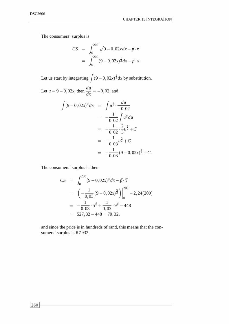
DSC2606
CHAPTER 15 INTEGRATION
The consumers’ surplus is
CS =∫ 200
0
√
9−0,02xdx− p̄ · x̄
=∫ 200
0(9−0,02x)
12 dx− p̄ · x̄.
Let us start by integrating∫
(9−0,02x)12dxby substitution.
Let u= 9−0,02x, thendudx
=−0,02, and
∫
(9−0,02x)12dx =
∫
u12 · du−0,02
= − 10,02
∫
u12du
= − 10,02
· 23
u32 +C
= − 10,03
u32 +C
= − 10,03
(9−0,02x)32 +C.
The consumers’ surplus is then
CS =
∫ 200
0(9−0,02x)
12dx− p̄ · x̄
=
(
− 10,03
(9−0,02x)32
)∣
∣
∣
∣
200
0−2,24(200)
= − 10,03
·532 +
10,03
·932 −448
= 527,32−448= 79,32,
and since the price is in hundreds of rand, this means that thecon-sumers’ surplus is R7932.
260
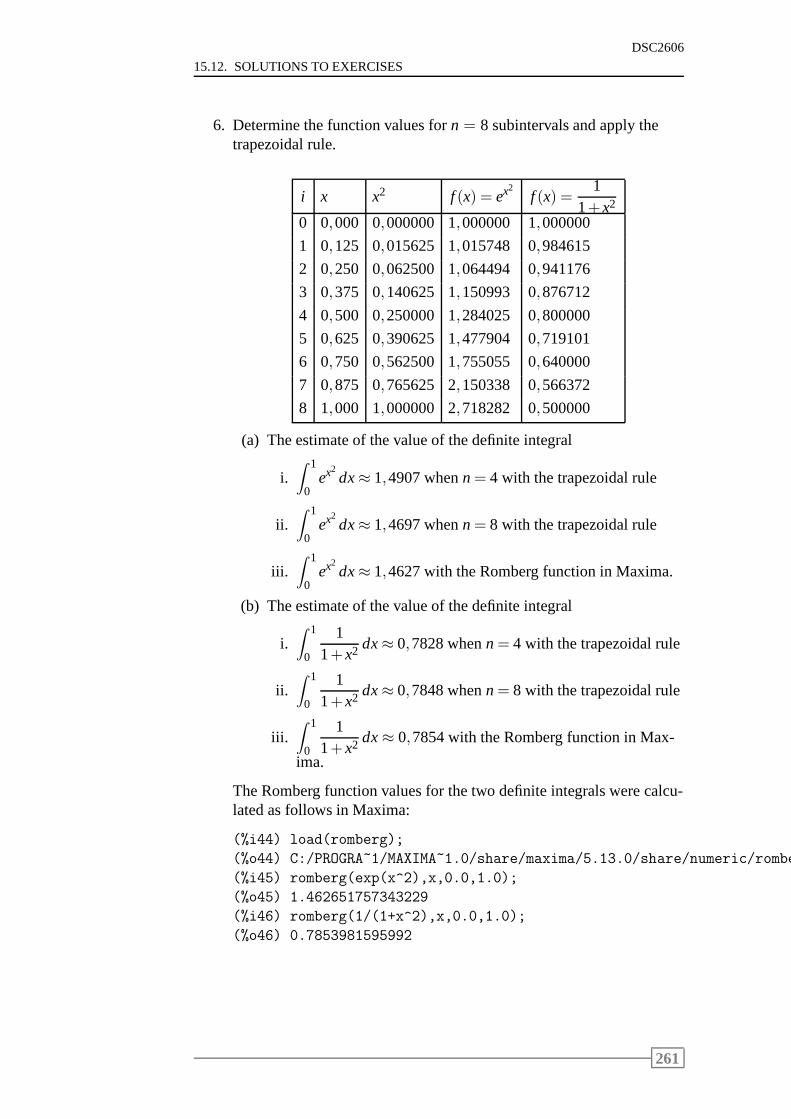
15.12. SOLUTIONS TO EXERCISES
DSC2606
6. Determine the function values forn = 8 subintervals and apply thetrapezoidal rule.
i x x2 f (x) = ex2f (x) =
11+x2
0 0,000 0,000000 1,000000 1,000000
1 0,125 0,015625 1,015748 0,984615
2 0,250 0,062500 1,064494 0,941176
3 0,375 0,140625 1,150993 0,876712
4 0,500 0,250000 1,284025 0,800000
5 0,625 0,390625 1,477904 0,719101
6 0,750 0,562500 1,755055 0,640000
7 0,875 0,765625 2,150338 0,566372
8 1,000 1,000000 2,718282 0,500000
(a) The estimate of the value of the definite integral
i.∫ 1
0ex2
dx≈ 1,4907 whenn= 4 with the trapezoidal rule
ii.∫ 1
0ex2
dx≈ 1,4697 whenn= 8 with the trapezoidal rule
iii.∫ 1
0ex2
dx≈ 1,4627 with the Romberg function in Maxima.
(b) The estimate of the value of the definite integral
i.∫ 1
0
11+x2 dx≈ 0,7828 whenn= 4 with the trapezoidal rule
ii.∫ 1
0
11+x2 dx≈ 0,7848 whenn= 8 with the trapezoidal rule
iii.∫ 1
0
11+x2 dx≈ 0,7854 with the Romberg function in Max-
ima.
The Romberg function values for the two definite integrals were calcu-lated as follows in Maxima:
(%i44) load(romberg);
(%o44) C:/PROGRA~1/MAXIMA~1.0/share/maxima/5.13.0/share/numeric/rombe
(%i45) romberg(exp(x^2),x,0.0,1.0);
(%o45) 1.462651757343229
(%i46) romberg(1/(1+x^2),x,0.0,1.0);
(%o46) 0.7853981595992
261

DSC2606
CHAPTER 15 INTEGRATION
262
Chapter 16
Partial differentiation
Contents16.1 Introduction . . . . . . . . . . . . . . . . . . . . . . . . 264
16.2 Partial derivatives . . . . . . . . . . . . . . . . . . . . . 266
16.3 Second-order partial derivatives . . . . . . . . . . . . . 272
16.4 The Cobb-Douglas production function . . . . . . . . . 275
16.5 Exercises . . . . . . . . . . . . . . . . . . . . . . . . . . 277
16.6 Solutions to exercises . . . . . . . . . . . . . . . . . . . 277
263
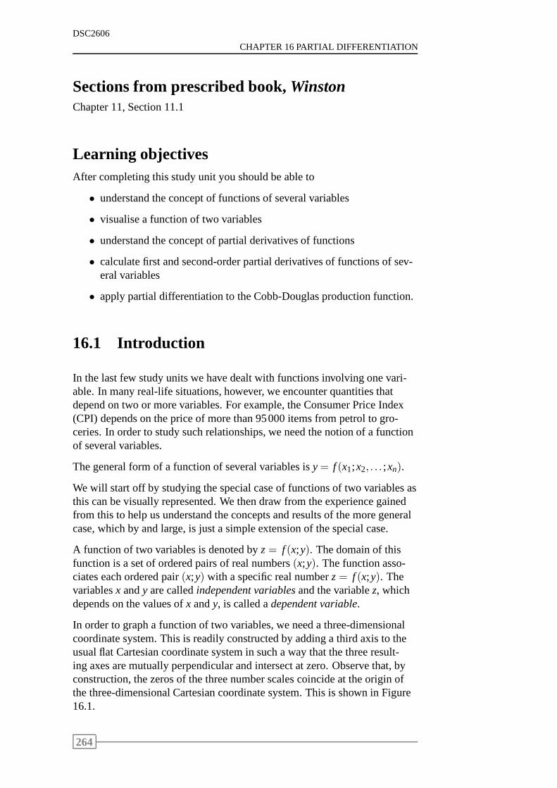
DSC2606
CHAPTER 16 PARTIAL DIFFERENTIATION
Sections from prescribed book,WinstonChapter 11, Section 11.1
Learning objectivesAfter completing this study unit you should be able to
• understand the concept of functions of several variables
• visualise a function of two variables
• understand the concept of partial derivatives of functions
• calculate first and second-order partial derivatives of functions of sev-eral variables
• apply partial differentiation to the Cobb-Douglas production function.
16.1 Introduction
In the last few study units we have dealt with functions involving one vari-able. In many real-life situations, however, we encounter quantities thatdepend on two or more variables. For example, the Consumer Price Index(CPI) depends on the price of more than 95000 items from petrol to gro-ceries. In order to study such relationships, we need the notion of a functionof several variables.
The general form of a function of several variables isy= f (x1;x2, . . . ;xn).
We will start off by studying the special case of functions oftwo variables asthis can be visually represented. We then draw from the experience gainedfrom this to help us understand the concepts and results of the more generalcase, which by and large, is just a simple extension of the special case.
A function of two variables is denoted byz= f (x;y). The domain of thisfunction is a set of ordered pairs of real numbers(x;y). The function asso-ciates each ordered pair(x;y) with a specific real numberz= f (x;y). Thevariablesx andy are calledindependent variablesand the variablez, whichdepends on the values ofx andy, is called adependent variable.
In order to graph a function of two variables, we need a three-dimensionalcoordinate system. This is readily constructed by adding a third axis to theusual flat Cartesian coordinate system in such a way that the three result-ing axes are mutually perpendicular and intersect at zero. Observe that, byconstruction, the zeros of the three number scales coincideat the origin ofthe three-dimensional Cartesian coordinate system. This is shown in Figure16.1.
264
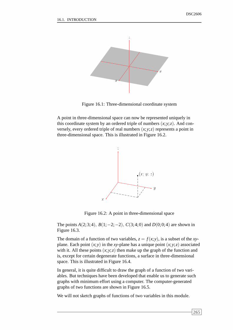
16.1. INTRODUCTION
DSC2606
x
y
z
1
Figure 16.1: Three-dimensional coordinate system
A point in three-dimensional space can now be represented uniquely inthis coordinate system by an ordered triple of numbers(x;y;z). And con-versely, every ordered triple of real numbers(x;y;z) represents a point inthree-dimensional space. This is illustrated in Figure 16.2.
(x; y; z)
b
x
y
z
1
Figure 16.2: A point in three-dimensional space
The pointsA(2;3;4), B(1;−2;−2), C(3;4;0) andD(0;0;4) are shown inFigure 16.3.
The domain of a function of two variables,z= f (x;y), is a subset of thexy-plane. Each point(x;y) in thexy-plane has a unique point(x;y;z) associatedwith it. All these points(x;y;z) then make up the graph of the function andis, except for certain degenerate functions, a surface in three-dimensionalspace. This is illustrated in Figure 16.4.
In general, it is quite difficult to draw the graph of a function of two vari-ables. But techniques have been developed that enable us to generate suchgraphs with minimum effort using a computer. The computer-generatedgraphs of two functions are shown in Figure 16.5.
We will not sketch graphs of functions of two variables in this module.
265

DSC2606
CHAPTER 16 PARTIAL DIFFERENTIATION
x
y
z
b
A (2; 3; 4)
b
C (3; 4; 0)
b
B (1; �2; �2)
b
D (0; 0; 4)
1
Figure 16.3: Four points in three-dimensional space
−2
−1
0
1
2
−2
−1
0
1
2−0.5
0
0.5
.
.
(x; y; z)
z
y x
Figure 16.4: Graph ofz= f (x; y)
16.2 Partial derivatives
For a function of one variable,y= f (x), the rate of change with respect toxmeans the change in the function for movement along thex-axis. As seen inprevious study units, this is measured by the slope of the tangent line to thecurvey = f (x) through the point(x;y) and is called the derivative off (x)with respect tox.
For a function of two variables,z= f (x;y), the rate of change off (x;y) canbe either with respect tox, where the change is along thex-axis, or with re-spect toy, where the change is along they-axis.
As seen before, the functionz= f (x;y) is a surface in three-dimensionalspace. Suppose we want to study the rate of change of this function with
266
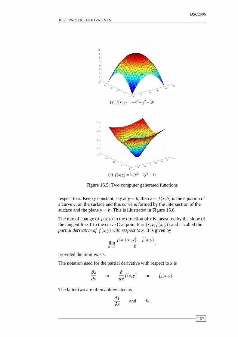
16.2. PARTIAL DERIVATIVES
DSC2606
05
1015
2025
0
5
10
15
20
252
3
4
5
6
7
8
9
10
(a) f (x; y) =−x2− y2+10
05
1015
2025
3035
0
10
20
30
400
0.5
1
1.5
2
2.5
3
3.5
(b) f (x; y) = ln(x2−2y2+1)
Figure 16.5: Two computer generated functions
respect tox. Keepy constant, say aty= b, thenz= f (x;b) is the equation ofa curve C on the surface and this curve is formed by the intersection of thesurface and the planey= b. This is illustrated in Figure 16.6.
The rate of change off (x;y) in the direction ofx is measured by the slope ofthe tangent line T to the curve C at point P= (x;y; f (x;y)) and is called thepartial derivative of f(x;y) with respect to x. It is given by
limh→0
f (x+h;y)− f (x;y)h
,
provided the limit exists.
The notation used for the partial derivative with respect tox is
∂z∂x
or∂∂x
f (x;y) or fx(x;y).
The latter two are often abbreviated as
∂ f∂x
and fx.
267
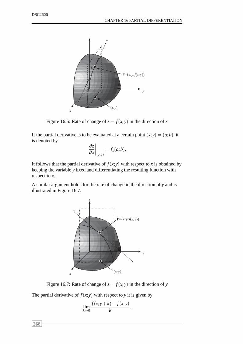
DSC2606
CHAPTER 16 PARTIAL DIFFERENTIATION
z
y
x
b
( x ; y )
C
P = ( x ; y ; f ( x ; y ) )
T
Figure 16.6: Rate of change ofz= f (x;y) in the direction ofx
If the partial derivative is to be evaluated at a certain point (x;y) = (a;b), itis denoted by
∂z∂x
∣
∣
∣
∣
(a;b)= fx(a;b).
It follows that the partial derivative off (x;y) with respect tox is obtained bykeeping the variabley fixed and differentiating the resulting function withrespect tox.
A similar argument holds for the rate of change in the direction ofy and isillustrated in Figure 16.7.
y
x
z
C
a
T
( x ; y )
P = ( x ; y ; f ( x ; y ) )
Figure 16.7: Rate of change ofz= f (x;y) in the direction ofy
The partial derivative off (x;y) with respect toy it is given by
limk→0
f (x;y+k)− f (x;y)k
,
268
16.2. PARTIAL DERIVATIVES
DSC2606
provided the limit exists.
The notation used for the partial derivative with respect toy is
∂z∂y
or∂∂y
f (x;y) or fy(x;y).
The latter two are often abbreviated as
∂ f∂y
and fy.
If the partial derivative is to be evaluated at a certain point (x;y) = (a;b), itis denoted by
∂z∂y
∣
∣
∣
∣
(a;b)= fy(a;b).
To calculate the partial derivative of a function of severalvariables with re-spect to one variable, sayx, we think of the other variables as if they wereconstants and differentiate the resulting function with respect tox, using therules for differentiation as discussed in Study unit 9.
Example 16.1
Consider the functionf (x;y) = x2−xy2+y3.
(a) Calculate the partial derivatives off (x;y).
(b) What is the rate of change of the functionf (x;y) in thex-directionat point(1;2)?
(c) What is the rate of change of the functionf (x;y) in they-directionat point(1;2)?
Solution
(a) To calculate∂ f∂x
, think of the variabley as a constant and differentiate
the resulting function ofx with respect tox. Then
∂ f∂x
= 2x−y2+0= 2x−y2.
To calculate∂ f∂y
, think of the variablex as a constant and differentiate
the resulting function ofy with respect toy. Then
∂ f∂y
= 0−x×2y+3y2 =−2xy+3y2.
269
DSC2606
CHAPTER 16 PARTIAL DIFFERENTIATION
(b) The rate of change of the functionf (x;y) in thex-direction at point(1;2) is given by
fx(1;2) =∂ f∂x
∣
∣
∣
∣
(1;2)= 2(1)−22 =−2,
that is, f (x;y) decreases by two units for each unit increase in thex-direction,y being kept constant aty= 2.
(c) The rate of change of the functionf (x;y) in they-direction at point(1;2) is given by
fy(1;2) =∂ f∂y
∣
∣
∣
∣
(1;2)=−2(1)(2)+3(2)2= 8,
that is, f (x;y) increases by 8 units for each unit increase in they-direction,x being kept constant atx= 1.
Example 16.2
Calculate the partial derivatives of each of the following functions:
(a) f (x;y) =xy
x2+y2
(b) g(s; t) = (s2−st+ t3)5
(c) h(u;v) = eu2−2v2
(d) f (x;y) = ln(x2+2y2)
(e) f (x;y;z) = xyz−xeyz+xlny
Solution
(a) Nowf (x;y) =
xyx2+y2 = xy(x2+y2)−1.
To calculate∂ f∂x
, think of the variabley as if it were a constant. Then
by the product rule
∂ f∂x
= xy[−(x2+y2)−2×2x]+ (x2+y2)−1(y)
=−2x2y
(x2+y2)2 +y
x2+y2
=−2x2y+yx2+y3
(x2+y2)2
=y(y2−x2)
(x2+y2)2 .
270
16.2. PARTIAL DERIVATIVES
DSC2606
To calculate∂ f∂y
, think of the variablex as if it were a constant. Then
∂ f∂y
= xy[−(x2+y2)−2×2y]+ (x2+y2)−1(x)
=−2xy2
(x2+y2)2 +x
x2+y2
=−2xy2+x3+xy2
(x2+y2)2
=x(x2−y2)
(x2+y2)2 .
(b) To calculate∂g∂s
, we treat the variablet as if it were a constant. Then
by the power rule
∂g∂s
= 5(s2−st+ t3)4 · (2s− t)
= 5(2s− t)(s2−st+ t3)4.
To calculate∂g∂ t
, we treat the variables as if it were a constant. Then
∂g∂ t
= 5(s2−st+ t3)4 · (−s+3t2)
= 5(3t2−s)(s2−st+ t3)4.
(c) To calculate∂h∂u
, we treat the variablev as if it were a constant. Then
by the chain rule for exponential functions
∂h∂u
= eu2−2v2×2u
= 2ueu2−2v2.
To calculate∂h∂v
, we treat the variableu as if it were a constant. Then
∂h∂v
= eu2−2v2 · [−2(2v)]
= −4veu2−2v2.
(d) To calculate∂ f∂x
, we treat the variabley as if it were a constant. Then
by the chain rule for logarithmic functions
∂ f∂x
=2x
x2+2y2 .
271
DSC2606
CHAPTER 16 PARTIAL DIFFERENTIATION
To calculate∂ f∂y
, we treat the variablex as if it were a constant. Then
∂ f∂y
=4y
x2+2y2 .
(e) Here we have a function of three variablesx, y andz, and we are re-quired to find all three the partial derivativesfx, fy and fz.
To calculatefx, we think of the other two variabley andzas if theywere constants. Then
fx = yz−eyz+ lny.
To calculatefy, we think of the other two variablex andzas if theywere constants. Then
fy = xz−xzeyz+xy.
To calculatefz, we think of the other two variablex andy as if theywere constants. Then
fz = xy−xyeyz.
16.3 Second-order partial derivatives
The partial derivatives that we have considered up till now are also known asfirst-order partial derivatives.
If we consider a function of two variablesx andy, z= f (x;y), then the first-order partial derivatives,fx(x;y) and fy(x;y), are also functions of the twovariablesx andy. We may differentiate each of these functions,fx and fy, toobtain thesecond-order partial derivativesof f (x;y).
Therefore, differentiating the functionfx(x;y) with respect tox leads to thesecond-order partial derivative
fxx(x;y) =∂∂x
[ fx(x;y)] .
This is often abbreviated to
fxx or∂∂x
( fx) or∂ 2 f
∂x2 .
Differentiating the functionfx(x;y) with respect toy leads to the second-order partial derivative
fxy(x;y) =∂∂y
[ fx(x;y)] ,
272
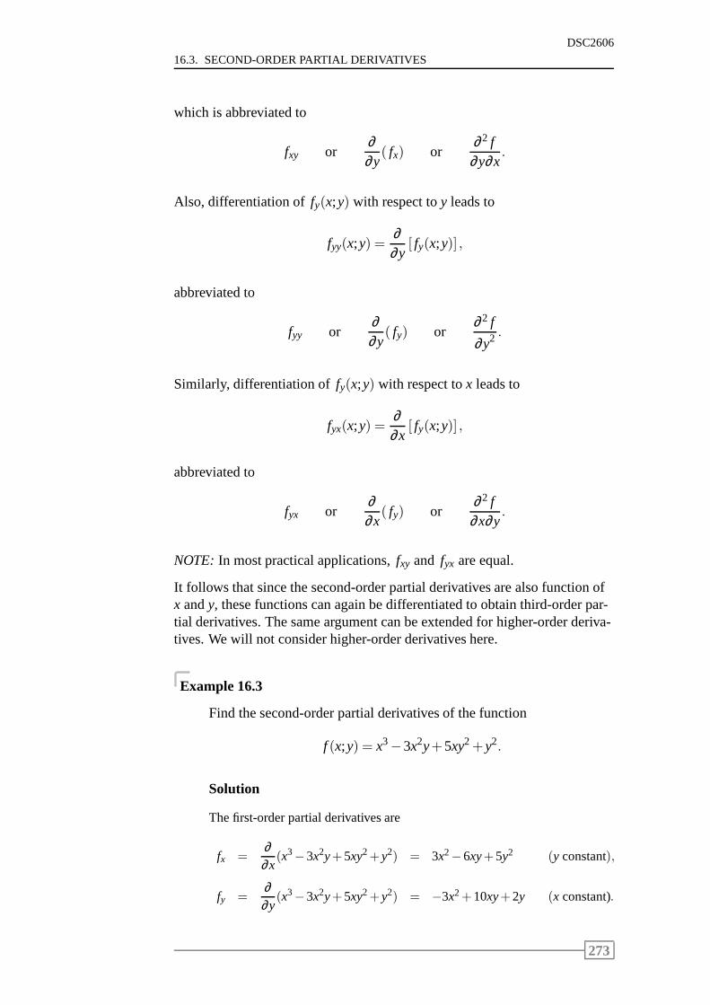
16.3. SECOND-ORDER PARTIAL DERIVATIVES
DSC2606
which is abbreviated to
fxy or∂∂y
( fx) or∂ 2 f
∂y∂x.
Also, differentiation offy(x;y) with respect toy leads to
fyy(x;y) =∂∂y
[ fy(x;y)] ,
abbreviated to
fyy or∂∂y
( fy) or∂ 2 f
∂y2 .
Similarly, differentiation offy(x;y) with respect tox leads to
fyx(x;y) =∂∂x
[ fy(x;y)] ,
abbreviated to
fyx or∂∂x
( fy) or∂ 2 f
∂x∂y.
NOTE: In most practical applications,fxy and fyx are equal.
It follows that since the second-order partial derivativesare also function ofx andy, these functions can again be differentiated to obtain third-order par-tial derivatives. The same argument can be extended for higher-order deriva-tives. We will not consider higher-order derivatives here.
Example 16.3
Find the second-order partial derivatives of the function
f (x;y) = x3−3x2y+5xy2+y2.
Solution
The first-order partial derivatives are
fx =∂∂x
(x3−3x2y+5xy2+y2) = 3x2−6xy+5y2 (y constant),
fy =∂∂y
(x3−3x2y+5xy2+y2) = −3x2+10xy+2y (x constant).
273
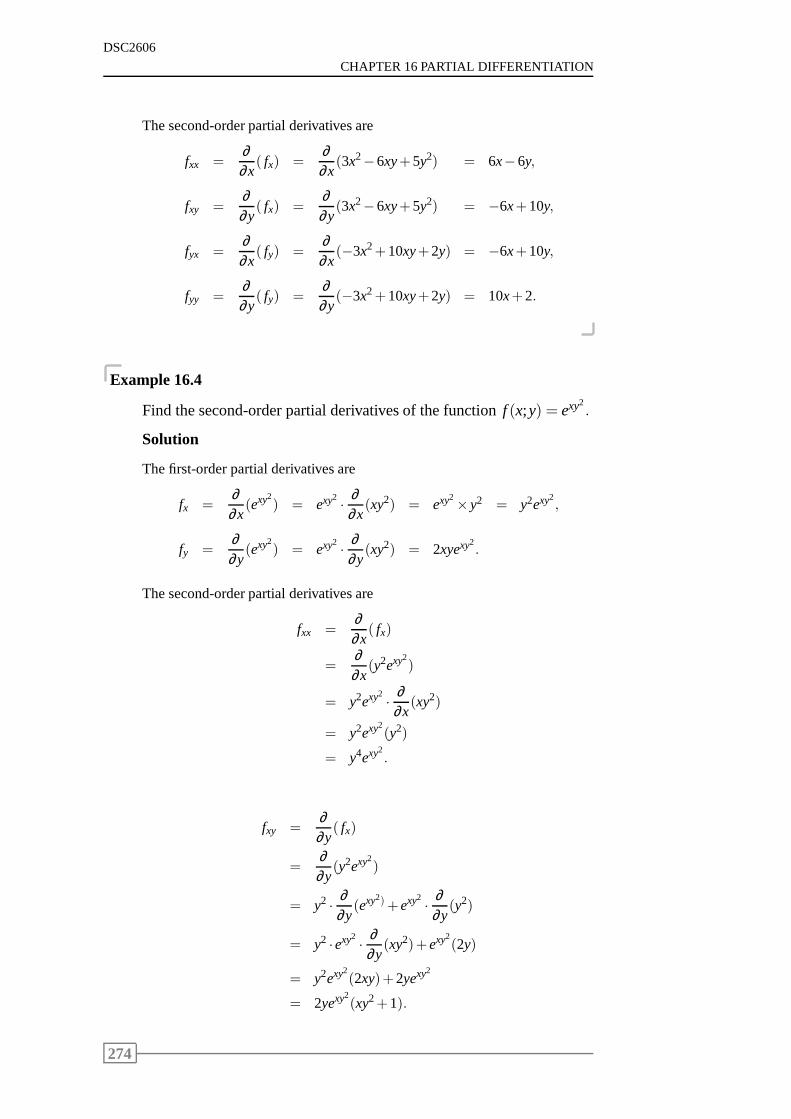
DSC2606
CHAPTER 16 PARTIAL DIFFERENTIATION
The second-order partial derivatives are
fxx =∂∂x
( fx) =∂∂x
(3x2−6xy+5y2) = 6x−6y,
fxy =∂∂y
( fx) =∂∂y
(3x2−6xy+5y2) = −6x+10y,
fyx =∂∂x
( fy) =∂∂x
(−3x2+10xy+2y) = −6x+10y,
fyy =∂∂y
( fy) =∂∂y
(−3x2+10xy+2y) = 10x+2.
Example 16.4
Find the second-order partial derivatives of the functionf (x;y) = exy2.
Solution
The first-order partial derivatives are
fx =∂∂x
(exy2) = exy2 · ∂
∂x(xy2) = exy2×y2 = y2exy2
,
fy =∂∂y
(exy2) = exy2 · ∂
∂y(xy2) = 2xyexy2
.
The second-order partial derivatives are
fxx =∂∂x
( fx)
=∂∂x
(y2exy2)
= y2exy2 · ∂∂x
(xy2)
= y2exy2(y2)
= y4exy2.
fxy =∂∂y
( fx)
=∂∂y
(y2exy2)
= y2 · ∂∂y
(exy2)+exy2 · ∂∂y
(y2)
= y2 ·exy2 · ∂∂y
(xy2)+exy2(2y)
= y2exy2(2xy)+2yexy2
= 2yexy2(xy2+1).
274
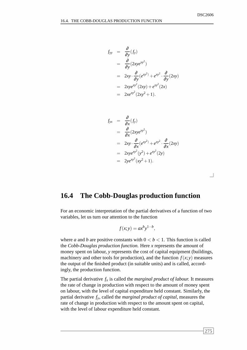
16.4. THE COBB-DOUGLAS PRODUCTION FUNCTION
DSC2606
fyy =∂∂y
( fy)
=∂∂y
(2xyexy2)
= 2xy· ∂∂y
(exy2)+exy2 · ∂∂y
(2xy)
= 2xyexy2(2xy)+exy2
(2x)
= 2xexy2(2xy2+1).
fyx =∂∂x
( fy)
=∂∂x
(2xyexy2)
= 2xy· ∂∂x
(exy2)+exy2 · ∂∂x
(2xy)
= 2xyexy2(y2)+exy2
(2y)
= 2yexy2(xy2+1).
16.4 The Cobb-Douglas production function
For an economic interpretation of the partial derivatives of a function of twovariables, let us turn our attention to the function
f (x;y) = axby1−b,
wherea andb are positive constants with 0< b< 1. This function is calledtheCobb-Douglas production function.Herex represents the amount ofmoney spent on labour,y represents the cost of capital equipment (buildings,machinery and other tools for production), and the functionf (x;y) measuresthe output of the finished product (in suitable units) and is called, accord-ingly, the production function.
The partial derivativefx is called themarginal product of labour.It measuresthe rate of change in production with respect to the amount ofmoney spenton labour, with the level of capital expenditure held constant. Similarly, thepartial derivativefy, called themarginal product of capital, measures therate of change in production with respect to the amount spenton capital,with the level of labour expenditure held constant.
275
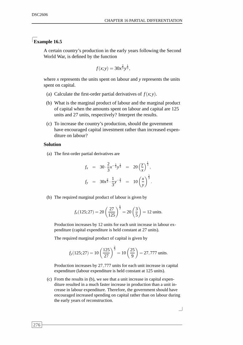
DSC2606
CHAPTER 16 PARTIAL DIFFERENTIATION
Example 16.5
A certain country’s production in the early years followingthe SecondWorld War, is defined by the function
f (x;y) = 30x23 y
13 ,
wherex represents the units spent on labour andy represents the unitsspent on capital.
(a) Calculate the first-order partial derivatives off (x;y).
(b) What is the marginal product of labour and the marginal productof capital when the amounts spent on labour and capital are 125units and 27 units, respectively? Interpret the results.
(c) To increase the country’s production, should the governmenthave encouraged capital investment rather than increased expen-diture on labour?
Solution
(a) The first-order partial derivatives are
fx = 30· 23
x−13 y
13 = 20
(yx
)13,
fy = 30x23 · 1
3y−
23 = 10
(
xy
)23
.
(b) The required marginal product of labour is given by
fx(125;27) = 20
(
27125
)13
= 20
(
35
)
= 12 units.
Production increases by 12 units for each unit increase in labour ex-penditure (capital expenditure is held constant at 27 units).
The required marginal product of capital is given by
fy(125;27) = 10
(
12527
)23
= 10
(
259
)
= 27,777 units.
Production increases by 27,777 units for each unit increase in capitalexpenditure (labour expenditure is held constant at 125 units).
(c) From the results in (b), we see that a unit increase in capital expen-diture resulted in a much faster increase in production thana unit in-crease in labour expenditure. Therefore, the government should haveencouraged increased spending on capital rather than on labour duringthe early years of reconstruction.
276
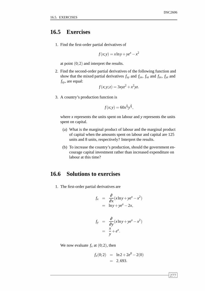
16.5. EXERCISES
DSC2606
16.5 Exercises
1. Find the first-order partial derivatives of
f (x;y) = xlny+yex−x2
at point(0;2) and interpret the results.
2. Find the second-order partial derivatives of the following function andshow that the mixed partial derivativesfxy and fyx, fxz and fzx, fyz andfzy, are equal:
f (x;y;z) = 3xyz2+x2yz.
3. A country’s production function is
f (x;y) = 60x13 y
23 ,
wherex represents the units spent on labour andy represents the unitsspent on capital.
(a) What is the marginal product of labour and the marginal productof capital when the amounts spent on labour and capital are 125units and 8 units, respectively? Interpret the results.
(b) To increase the country’s production, should the government en-courage capital investment rather than increased expenditure onlabour at this time?
16.6 Solutions to exercises
1. The first-order partial derivatives are
fx =∂∂x
(xlny+yex−x2)
= lny+yex−2x,
fy =∂∂y
(xlny+yex−x2)
=xy+ex.
We now evaluatefx at (0;2), then
fx(0;2) = ln2+2e0−2(0)
= 2,693.
277
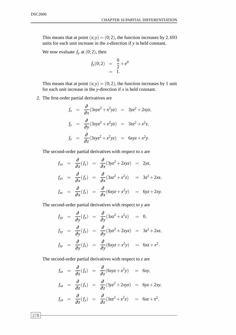
DSC2606
CHAPTER 16 PARTIAL DIFFERENTIATION
This means that at point(x;y) = (0;2), the function increases by 2,693units for each unit increase in thex-direction ify is held constant.
We now evaluatefy at (0;2), then
fy(0;2) =02+e0
= 1.
This means that at point(x;y) = (0;2), the function increases by 1 unitfor each unit increase in they-direction ifx is held constant.
2. The first-order partial derivatives are
fx =∂∂x
(3xyz2+x2yz) = 3yz2+2xyz,
fy =∂∂y
(3xyz2+x2yz) = 3xz2+x2z,
fz =∂∂z
(3xyz2+x2yz) = 6xyz+x2y.
The second-order partial derivatives with respect tox are
fxx =∂∂x
( fx) =∂∂x
(3yz2+2xyz) = 2yz,
fyx =∂∂x
( fy) =∂∂x
(3xz2+x2z) = 3z2+2xz,
fzx =∂∂x
( fz) =∂∂x
(6xyz+x2y) = 6yz+2xy.
The second-order partial derivatives with respect toy are
fyy =∂∂y
( fy) =∂∂y
(3xz2+x2z) = 0,
fxy =∂∂y
( fx) =∂∂y
(3yz2+2xyz) = 3z2+2xz,
fzy =∂∂y
( fz) =∂∂y
(6xyz+x2y) = 6xz+x2.
The second-order partial derivatives with respect toz are
fzz =∂∂z
( fz) =∂∂z
(6xyz+x2y) = 6xy,
fxz =∂∂z
( fx) =∂∂z
(3yz2+2xyz) = 6yz+2xy,
fyz =∂∂z
( fy) =∂∂z
(3xz2+x2z) = 6xz+x2.
278
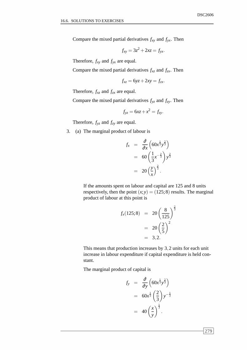
16.6. SOLUTIONS TO EXERCISES
DSC2606
Compare the mixed partial derivativesfxy and fyx. Then
fxy = 3z2+2xz= fyx.
Therefore,fxy and fyx are equal.
Compare the mixed partial derivativesfxz and fzx. Then
fxz= 6yz+2xy= fzx.
Therefore,fxz and fzx are equal.
Compare the mixed partial derivativesfyz and fzy. Then
fyz= 6xz+x2 = fzy.
Therefore,fyz and fzy are equal.
3. (a) The marginal product of labour is
fx =∂∂x
(
60x13y
23
)
= 60
(
13
x−23
)
y23
= 20(y
x
)23.
If the amounts spent on labour and capital are 125 and 8 unitsrespectively, then the point(x;y) = (125;8) results. The marginalproduct of labour at this point is
fx(125;8) = 20
(
8125
)23
= 20
(
25
)2
= 3,2.
This means that production increases by 3,2 units for each unitincrease in labour expenditure if capital expenditure is held con-stant.
The marginal product of capital is
fy =∂∂y
(
60x13y
23
)
= 60x13
(
23
)
y−13
= 40
(
xy
)13
.
279
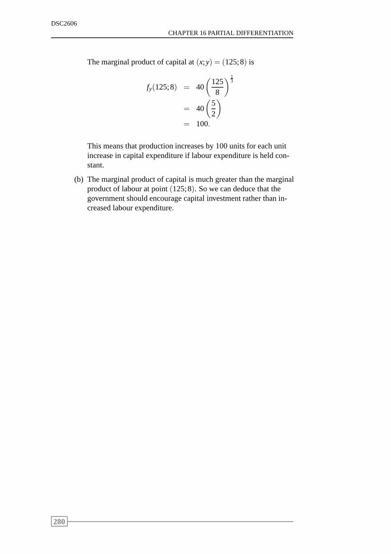
DSC2606
CHAPTER 16 PARTIAL DIFFERENTIATION
The marginal product of capital at(x;y) = (125;8) is
fy(125;8) = 40
(
1258
)13
= 40
(
52
)
= 100.
This means that production increases by 100 units for each unitincrease in capital expenditure if labour expenditure is held con-stant.
(b) The marginal product of capital is much greater than the marginalproduct of labour at point(125;8). So we can deduce that thegovernment should encourage capital investment rather than in-creased labour expenditure.
280

Chapter 17
Optimisation of NLPs in severalvariables
Contents17.1 Introduction . . . . . . . . . . . . . . . . . . . . . . . . 282
17.2 Convex and concave functions . . . . . . . . . . . . . . 283
17.3 Stationary points and the nature of stationary points .. 287
17.4 Solving NLPs in several variables by differential calcu-lus . . . . . . . . . . . . . . . . . . . . . . . . . . . . . . 289
17.5 Exercises . . . . . . . . . . . . . . . . . . . . . . . . . . 293
17.6 Solutions to exercises . . . . . . . . . . . . . . . . . . . 294
281
DSC2606
CHAPTER 17 OPTIMISATION OF NLPS IN SEVERAL VARIABLES
Sections from prescribed book,WinstonChapter 2, Section 2.1Chapter 2, Section 2.6Chapter 11, Section 11.3Chapter 11, Section 11.6
Learning objectivesAfter completing this study unit you should be able to
• explain the concepts of the Hessian, the principal minors, the leadingprincipal minors and the determinant of a matrix
• set up the Hessian matrix of a function of several variables
• determine the principal minors and the leading principal minors of amatrix
• determine the convexity/concavity of a function
• determine the stationary points of a function of several variables
• determine the nature of the stationary points: local (or relative) mini-mum, maximum or saddle points
• use the convexity/concavity of the objective function to determinewhether a local extremum is an absolute extremum; in other words,whether the solution obtained is in fact the optimal solution
• solve NLP models in several variables by means of differential calcu-lus.
17.1 Introduction
In previous study units we saw that many practical problems were formu-lated as functions of one variable. Such functions were thensolved by de-termining their extreme values. For example, the problem offinding a firm’sproduction level,x, that will yield maximum profit was solved by finding theabsolute maximum value of the profit functionP(x).
The notion of an extreme value of a function plays an equally important rolein the case of a function of several variables. As in the case of a function ofone variable, it is important to distinguish between the concept of a relativemaximum (relative minimum) and that of an absolute maximum (absoluteminimum) of the function. A relative extremum (relative maximum or rela-tive minimum) may or may not be an absolute extremum.
282
17.2. CONVEX AND CONCAVE FUNCTIONS
DSC2606
Just as the first and second-order derivatives play an important role in de-termining the relative extrema of a function of one variable, the first andsecond-order partial derivatives are powerful tools for locating and classi-fying the relative extrema of functions of several variables, as we shall seelater in this study unit.
We also saw in previous study units that there is no guaranteethat the solu-tion obtained to an NLP model (whether by hand or by computer)is actuallythe optimal solution to the model. This contributes to the fact that NLP mod-els are much harder to solve than LP models.
It is important that we know the criteria that must apply before we can de-duce that the solution obtained is indeed the optimal solution. The convex-ity/concavity of a function gives such criteria. We discussed this for func-tions of one variable in Study unit 13. We saw that the second-order deriva-tive of a function is used to determine the convexity/concavity of the func-tion. Now we extend our study to functions of several variables.
17.2 Convex and concave functions
Functions of several variables do not have only one second-order derivative.A function ofn variables hasn2 second-order partial derivatives. For exam-ple, a function of two variables, sayg(x1;x2), has four second-order partialderivatives, namely
∂ 2
∂x21
g(x1;x2);∂ 2
∂x2∂x1g(x1;x2);
∂ 2
∂x22
g(x1;x2);∂ 2
∂x1∂x2g(x1;x2).
Second-order partial derivatives as well as the following concepts are usedin the theorems that establish the convexity/concavity of functions of severalvariables:
• theHessianmatrix of a function
• the ith principal minorof a matrix
• thekth leading principal minorof a matrix.
Refer to the second half ofWinston, Section 11.3 for the definitions of theseconcepts and the theorems on convexity/concavity. Examples are also givento illustrate these definitions and theorems.
To understand the definitions of these concepts, you may needto refreshyour memory on basic algebra, especially onmatricesanddeterminants.Refer toWinston, Sections 2.1 and 2.6 for this.
283
DSC2606
CHAPTER 17 OPTIMISATION OF NLPS IN SEVERAL VARIABLES
Determining the convexity/concavity of functions is important and we illus-trate this by means of additional examples. These examples are taken fromthe problems at the end ofWinston, Section 11.3.
Example 17.1
Determine whether the functionf (x) =1x
is convex, concave or nei-
ther on the setS= (0;∞).
Solution
The derivatives are
f ′(x) =∂∂x
(x−1) = −x−2 = − 1x2 ,
f ′′(x) =∂∂x
(−x−2) = 2x−3 =2x3 .
Now f ′′(x) =2x3 > 0 for x∈ S= (0;∞).
Therefore,f (x) =1x
is a convex function onS.
Example 17.2
Determine whether the functionf (x1;x2) = x31+3x1x2+x2
2 is convex,concave or neither on the setS= R2.
Solution
The first-order partial derivatives are
∂ f∂x1
= 3x21+3x2,
∂ f∂x2
= 3x1+2x2.
The second-order partial derivatives are
∂ 2 f
∂x12 =
∂∂x1
(3x21+3x2) = 6x1,
∂ 2 f∂x2∂x1
=∂
∂x2(3x2
1+3x2) = 3,
∂ 2 f
∂x22 =
∂∂x2
(3x1+2x2) = 2,
∂ 2 f∂x1∂x2
=∂
∂x1(3x1+2x2) = 3.
284
17.2. CONVEX AND CONCAVE FUNCTIONS
DSC2606
The Hessian matrix is
H(x1;x2) =
[
6x1 3
3 2
]
.
The first principal minors are 6x1 and 2. Now 6x1 > 0 for x1 > 0 and 6x1 < 0for x1 < 0.
Therefore, the two theorems for convexity/concavity do nothold forx∈ S=R2. We conclude that the function is neither convex nor concaveonS= R2.
Example 17.3
Determine whether the functionf (x1;x2;x3) = −x21− x2
2− 2x23 +
0,5x1x2 is convex, concave or neither on the setS= R3.
Solution
The first-order partial derivatives are
∂ f∂x1
= −2x1+0,5x2,
∂ f∂x2
= −2x2+0,5x1,
∂ f∂x3
= −4x3.
The second-order partial derivatives are
∂ 2 f
∂x12 = −2,
∂ 2 f∂x2∂x1
= 0,5,∂ 2 f
∂x3∂x1= 0,
∂ 2 f
∂x22 = −2,
∂ 2 f∂x1∂x2
= 0,5,∂ 2 f
∂x3∂x2= 0,
∂ 2 f
∂x32 = −4,
∂ 2 f∂x1∂x3
= 0,∂ 2 f
∂x2∂x3= 0.
Notice that the following mixed partial derivatives are equivalent:
fx1x2 = 0,5 = fx2x1,
fx1x3 = 0 = fx3x1,
fx2x3 = 0 = fx3x2.
The Hessian matrix is
H(x1;x2;x3) =
−2 0,5 0
0,5 −2 0
0 0 −4
.
285
DSC2606
CHAPTER 17 OPTIMISATION OF NLPS IN SEVERAL VARIABLES
The first principal minors are−2,−2 and−4, all with the same sign as(−1)1 =−1.
The second principal minors are∣
∣
∣
∣
−2 0
0 −4
∣
∣
∣
∣
= (−2)(−4)−0= 8> 0,
∣
∣
∣
∣
−2 0
0 −4
∣
∣
∣
∣
= 8> 0,
∣
∣
∣
∣
−2 0,5
0,5 −2
∣
∣
∣
∣
=(−2)(−2)−(0,5)(0,5)=3,75> 0.
All have the same sign as(−1)2 =+1.
The third principal minor is the determinant of the Hessian matrix. Let
A=
−2 0,5 0
0,5 −2 0
0 0 −4
.
The determinant ofA can be obtained by expanding row 1 by means of co-factors. Then
detA = (−1)1+1a11detA11+(−1)1+2a12detA12+(−1)1+3a13detA13
= (−1)2(−2).
∣
∣
∣
∣
−2 0
0 −4
∣
∣
∣
∣
+ (−1)3(0,5).
∣
∣
∣
∣
0,5 0
0 −4
∣
∣
∣
∣
+ (−1)4(0).
∣
∣
∣
∣
0,5 −2
0 0
∣
∣
∣
∣
=−2(8)−0,5(−2)+0
=−16+1
=−15.
(Refer toWinston, Section 2.6 for determinants.)
This means that the third principal minor is−15< 0, and this has the samesign as(−1)3 =−1.
Therefore, we conclude that the function is a concave function onS= R3.
We now know how to determine the convexity/concavity of functions of sev-eral variables. This can be used to determine whether the solution to an NLPmodel is in fact the optimal solution. The criteria for this is given in two the-orems in the first part ofWinston, Section 11.3. These theorems are repeatedas two vital theorems in Section 13.2 of this study guide. Make sure that youare familiar with these theorems.
286
17.3. STATIONARY POINTS AND THE NATURE OF STATIONARY POINTS
DSC2606
17.3 Stationary points and the nature of station-ary points
Stationary points and the nature of stationary points, thatis, whether a sta-tionary point is a local maximum, a local minimum or a saddle point, arediscussed inWinston, Section 11.6. Turn to this section and study these con-cepts, the three important theorems and the examples.
Determining the stationary points of a function and the nature of these sta-tionary points is illustrated by means of examples.
Example 17.4
Find the relative extrema of the functionf (x;y) = 3x2−4xy+4y2−4x+8y+4.
Solution
The first-order partial derivatives are
fx =∂ f∂x
= 6x−4y−4,
fy =∂ f∂y
= −4x+8y+8.
The second-order partial derivatives are
∂ 2 f
∂x2 =∂∂x
( fx) =∂∂x
(6x−4y−4) = 6,
∂ 2 f∂y∂x
=∂∂y
( fx) =∂∂y
(6x−4y−4) = −4,
∂ 2 f
∂y2 =∂∂y
( fy) =∂∂y
(−4x+8y+8) = 8,
∂ 2 f∂x∂y
=∂∂x
( fy) =∂∂x
(−4x+8y+8) = −4.
To find the stationary points, we set∂ f∂x
= 0 and∂ f∂y
= 0 and solve the result-
ing equations simultaneously. Then
6x−4y−4 = 0 (1)
−4x+8y+8 = 0. (2)
Multiply equation (1) by 2. Then
12x−8y = 8 (3)
−4x+8y = −8. (4)
Add equations (3) and (4). Then
287
DSC2606
CHAPTER 17 OPTIMISATION OF NLPS IN SEVERAL VARIABLES
8x = 0
x = 0.
Substitute this into (3). Then
12(0)−8y = 8
y = −1.
The point(x;y) = (0;−1) is the only stationary point off (x;y).
The Hessian matrix is
H(x;y) =
[
6 −4
−4 8
]
.
The first leading principal minor isH1(x;y) = 6> 0.
The second leading principal minor isH2(x;y) = 6(8)− (−4)(−4)= 32> 0.
Both leading principal minors are>0. Therefore, the stationary point(0;−1)is a local minimum point.
Example 17.5
Find the relative extrema of the functionf (x;y) = 4y3+ x2−12y2−36y+2.
Solution
The first-order partial derivatives are
fx =∂ f∂x
= 2x,
fy =∂ f∂y
= 12y2−24y−36.
The second-order partial derivatives are
∂ 2 f
∂x2 = 2,∂ 2 f
∂y∂x= 0,
∂ 2 f
∂y2 = 24y−24,∂ 2 f
∂x∂y= 0.
To find the stationary points, we set∂ f∂x
= 0 and∂ f∂y
= 0. Then
2x= 0 ⇒ x= 0,
288
17.4. SOLVING NLPS IN SEVERAL VARIABLES BY DIFFERENTIAL CALCULUS
DSC2606
and12y2−24y−36 = 0
y2−2y−3 = 0
(y+1)(y−3) = 0
y=−1 or y= 3.
There are two stationary points:(0;−1) and(0;3).
The Hessian matrix is
H(x;y) =
[
2 0
0 24y−24
]
.
Consider point(x;y) = (0;−1).
The first leading principal minor isH1(x;y) = 2> 0.
The second leading principal minor isH2(x;y) = 2(24y−24)−0= 48y−48.And this evaluated at(0;−1) is
H2(0;−1) = 48(−1)−48=−96< 0.
The two theorems on local extrema do not hold. Since the leading principalminors are nonzero, we can conclude that(0;−1) is a saddle point.
Consider point(x;y) = (0;3).
The first leading principal minor isH1(x;y) = 2> 0.
The second leading principal minor evaluated at(0;3) is
H2(0;3) = 48(3)−48= 96> 0.
Now both leading principal minors are> 0. Therefore, the stationary point(0;3) is a local minimum point.
17.4 Solving NLPs in several variables by differ-ential calculus
To solve an NLP in several variables by differential calculus, we must carryout the following steps:
Step 1: Find the stationary points of the function under consideration.
Step 2: Determine the nature of the stationary points.
Step 3: Determine the convexity/concavity of the function.
289
DSC2606
CHAPTER 17 OPTIMISATION OF NLPS IN SEVERAL VARIABLES
Example 17.6
The Acrosonic Company produces and sells loudspeakers. Itstotalweekly revenue (in rand) is
R(x;y) =−14
x2− 38
y2− 14
xy+300x+240y.
Herex represents the number of fully assembled units andy representsthe number of assemble-it-yourself kits.
The total weekly cost (in rand) for the production of these loudspeak-ers is
C(x;y) = 180x+140y+5000.
Acrosonic wants to determine how many assembled units and howmany kits to produce per week to maximise its profit.
Solution
Decision variables
The decision variables are given as
x = number of fully assembled units produced weekly,y = number of assemble-it-yourself kits produced weekly.
Objective function
Profit must be maximised. Now
profit = revenue−cost
P(x;y) = R(x;y)−C(x;y)
= −14x2− 3
8y2− 14xy+300x+240y− (180x+140y+5000)
= −14x2− 3
8y2− 14xy+120x+100y−5000.
The objective function is
MaximiseP(x;y) =−14
x2− 38
y2− 14
xy+120x+100y−5000.
Constraints
The number of units produced cannot be negative; sox; y≥ 0.
The NLP model is
Maximise P(x;y) =−14x2− 3
8y2− 14xy+120x+100y−5000
subject to x; y≥ 0.
Solution
290
17.4. SOLVING NLPS IN SEVERAL VARIABLES BY DIFFERENTIAL CALCULUS
DSC2606
Step 1: Find the stationary points
The stationary points are determined fromPx = 0 andPy = 0 as
Px = −12x− 1
4y+120 = 0,
Py = −34y− 1
4x+100 = 0.
From this it follows that
2x+y = 480 (1)
x+3y = 400. (2)
Multiply equation (2) by−2. Then
−2x−6y = −800. (3)
Add equations (1) and (3). Then
−5y = −320
y = 64. (4)
Substitute (4) into (2). Then
x+3(64) = 400
x = 208.
The stationary point is at(x;y) = (208;64).
Step 2: Determine the nature of the stationary points
The second-order partial derivatives are
Pxx =−12, Pyx =−1
4,
Pyy =−34, Pxy =−1
4.
The Hessian matrix is
H(x;y) =
[ −12 −1
4
−14 −3
4
]
.
The first leading principal minor is−12 < 0, which has the same
sign as(−1)1 =−1.
The second leading principal minor is(−12)(−3
4)− (−14)(−1
4) =38− 1
16 =516 > 0, which has the same sign as(−1)2 =+1.
This means that(208;64) is a local maximum point.
Step 3: Determine convexity/concavity
The first principal minors are−12 and−3
4; both are negative andhave the same sign as(−1)1 =−1.
The second principal minor is516 > 0, which has the same sign as(−1)2 =+1.
From this it follows that the profit function is a concave function.
291
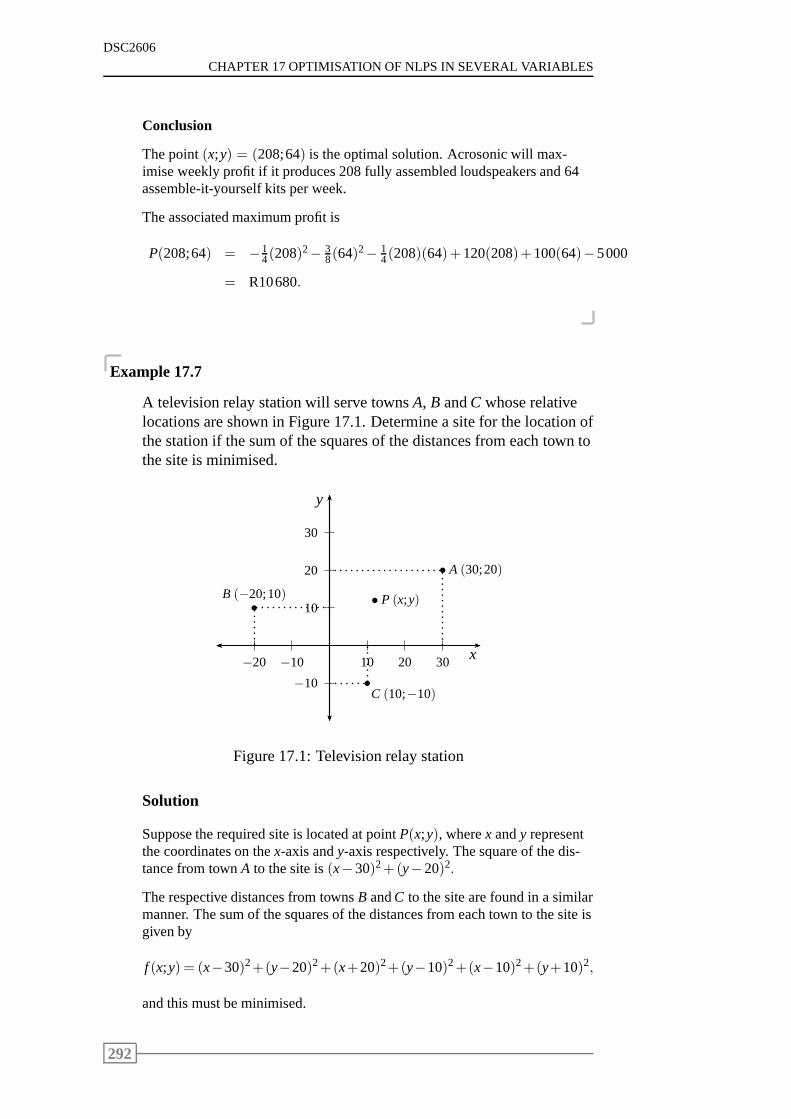
DSC2606
CHAPTER 17 OPTIMISATION OF NLPS IN SEVERAL VARIABLES
Conclusion
The point(x;y) = (208;64) is the optimal solution. Acrosonic will max-imise weekly profit if it produces 208 fully assembled loudspeakers and 64assemble-it-yourself kits per week.
The associated maximum profit is
P(208;64) = −14(208)2− 3
8(64)2− 14(208)(64)+120(208)+100(64)−5000
= R10680.
Example 17.7
A television relay station will serve townsA, B andC whose relativelocations are shown in Figure 17.1. Determine a site for the location ofthe station if the sum of the squares of the distances from each town tothe site is minimised.
10
20
30
−10
10 20 30−10−20
y
x
P (x;y)
A (30;20)
C (10;−10)
B (−20;10)
Figure 17.1: Television relay station
Solution
Suppose the required site is located at pointP(x;y), wherex andy representthe coordinates on thex-axis andy-axis respectively. The square of the dis-tance from townA to the site is(x−30)2+(y−20)2.
The respective distances from townsB andC to the site are found in a similarmanner. The sum of the squares of the distances from each townto the site isgiven by
f (x;y) = (x−30)2+(y−20)2+(x+20)2+(y−10)2+(x−10)2+(y+10)2,
and this must be minimised.
292
17.5. EXERCISES
DSC2606
The first-order partial derivatives are obtained by means ofthe chain rule as
∂ f∂x
= 2(x−30)+2(x+20)+2(x−10) = 6x−40,
∂ f∂y
= 2(y−20)+2(y−10)+2(y+10) = 6y−40.
Setting∂ f∂x
= 0 and∂ f∂y
= 0 gives
6x−40= 0 ⇒ x= 203 ,
6y−40= 0 ⇒ y= 203 .
The point(x;y) = (203 ; 20
3 ) is the only stationary point.
The second-order partial derivatives are
∂ 2 f
∂x2 = 6,∂ 2 f
∂y∂x= 0,
∂ 2 f
∂y2 = 6,∂ 2 f
∂x∂y= 0.
The Hessian matrix is
H(x;y) =
[
6 0
0 6
]
.
The first leading principal minor is 6> 0.
The second leading principal minor is 6(6)−0= 36> 0.
Both leading principal minors are nonnegative. Therefore,the point(203 ; 20
3 )is a local minimum.
The first principal minors are 6 and 6; both> 0.
The second principal minor is 36> 0.
All principal minors are> 0. Therefore, the function is convex.
We can conclude that the point(x;y) = (203 ; 20
3 ) is the optimal solution. Thismeans that the relay station should be located at a site with coordinatesx =203 andy = 20
3 . This will minimise the sum of the squared distances fromeach of the three towns to the site.
17.5 Exercises
1. Determine whether the function
f (x1;x2) =−x21−x1x2−2x2
2
293
DSC2606
CHAPTER 17 OPTIMISATION OF NLPS IN SEVERAL VARIABLES
is convex, concave or neither on the setS= R2.
(This problem is fromWinston, Section 11.3.)
2. Find all local maxima, local minima and saddle points for
f (x1;x2) = x31−3x1x2
2+x42.
(This problem is fromWinston, Section 11.6.)
3. A company can sell all it produces of a given output for R2 per unit.The output is produced by combining two inputs.
If q1 units of input 1 andq2 units of input 2 are used, the company can
produceq131 +q
232 units of the output.
If it costs R1 to purchase a unit of input 1 and R1,50 to purchase aunit of input 2, how can the company maximise its profit?
(This problem is fromWinston, Section 11.6.)
17.6 Solutions to exercises
1. The first-order partial derivatives are
∂ f∂x1
= −2x1−x2,
∂ f∂x2
= −x1−4x2.
The second-order partial derivatives are
∂ 2 f
∂x12 = −2,
∂ 2 f∂x2∂x1
=−1,
∂ 2 f
∂x22 = −4,
∂ 2 f∂x1∂x2
=−1.
The Hessian matrix is
H(x1;x2) =
[
−2 −1
−1 −4
]
.
The first principal minors are−2 and−4; both are negative and havethe same sign as(−1)1 =−1.
The second principal minor is(−2)(−4)−1= 7> 0; the same sign as(−1)2 =+1.
Therefore, the function is a concave function onS= R2.
294
17.6. SOLUTIONS TO EXERCISES
DSC2606
2. The first-order partial derivatives are
∂ f∂x1
= 3x21−3x2
2,
∂ f∂x2
= −6x1x2+4x32.
The second-order partial derivatives are
∂ 2 f
∂x12 = 6x1,
∂ 2 f∂x2∂x1
=−6x2,
∂ 2 f
∂x22 = −6x1+12x2
2,∂ 2 f
∂x1∂x2=−6x2.
Set∂ f∂x1
= 0, then
3x21−3x2
2 = 0
3(x1−x2)(x1+x2) = 0
x1−x2 = 0 or x1+x2 = 0
x1 = x2 or x1 =−x2.
Now substitutex1 = x2 into∂ f∂x2
= 0. Then
−6x1x2+4x32 = 0
−6x22+4x3
2 = 0
−2x22(3−2x2) = 0
x22 = 0 or 3−2x2 = 0
x2 = 0 or x2 =32.
Therefore,(0;0) and(32; 3
2) are stationary points.
Now substitutex1 =−x2 into∂ f∂x2
= 0. Then
−6x1x2+4x32 = 0
6x22+4x3
2 = 0
2x22(3+2x2) = 0
x22 = 0 or 3+2x2 = 0
x2 = 0 or x2 =−32.
Therefore,(0;0) and(32;−3
2) are stationary points.
295
DSC2606
CHAPTER 17 OPTIMISATION OF NLPS IN SEVERAL VARIABLES
The given function has three stationary points:(0;0), (32; 3
2) and(32;−3
2).
The Hessian matrix is
H(x1;x2) =
[
6x1 −6x2
−6x2 −6x1+12x22
]
.
The first leading principal minor is 6x1.
The second leading principal minor is
6x1(−6x1+12x22)− (−6x2)(−6x2)
=−36x21+72x1x2
2−36x22.
The leading principal minors must be evaluated at each of thestation-ary points.
Consider point(32; 3
2).
Now the first leading principal minor isH1(32; 3
2) = 6(32) = 9> 0.
The second leading principal minor is
H2(32; 3
2) = −36(32)
2+72(32)(
32)
2−36(32)
2
= 81> 0.
All leading principal minors are nonnegative. Therefore,(32; 3
2) is alocal minimum.
Consider point(32;−3
2).
We findH1(32;−3
2) = 9 > 0 andH2(32;−3
2) = 81> 0. Therefore,(3
2;−32) is also a local minimum.
Consider point(0;0).
We findH1(0;0) = 0 andH2(0;0) = 0. Therefore, we cannot deter-mine the nature of the stationary point(0;0).
3. Decision variables
The decision variables are given as
q1 = number of units of input 1 to be used,q2 = number of units of input 2 to be used.
Objective function
Profit must be maximised. Now
profit = revenue−cost
= 2(q131 +q
232 )− (q1+1,5q2).
296
17.6. SOLUTIONS TO EXERCISES
DSC2606
The objective function is then
Maximise f (q1;q2) = 2q131 +2q
232 −q1−1,5q2.
Constraints
A negative number of units of the two inputs cannot be used; soq1; q2≥0.
There are no other constraints.
The NLP model is
Maximise f (q1;q2) = 2q131 +2q
232 −q1−1,5q2
subject to q1; q2≥ 0.
Solution
The first-order partial derivatives are
∂ f∂q1
=23
q− 2
31 −1,
∂ f∂q2
=43
q− 1
32 −
32.
The second-order partial derivatives are
∂ 2 f
∂q12 = −4
9q− 5
31 ,
∂ 2 f∂q2∂q1
= 0,
∂ 2 f
∂q22 = −4
9q− 4
32 ,
∂ 2 f∂q1∂q2
= 0.
Set∂ f∂q1
= 0, then
23
q− 2
31 = 1
1
q231
=32
q231 =
23
q1 =
(
23
)32
.
297
DSC2606
CHAPTER 17 OPTIMISATION OF NLPS IN SEVERAL VARIABLES
Set∂ f∂q2
= 0, then
43
q− 1
32 =
32
1
q132
=98
q132 =
89
q2 =
(
89
)3
.
The function has the following stationary point:(q1;q2)=
(
(23
)32 ;(8
9
)3)
.
The Hessian matrix is
H(q1;q2) =
−49q− 5
31 0
0 −49q− 4
32
.
The first leading principal minor isH1(q1;q2) = −49q− 5
31 < 0, for q1 >
0, which has the same sign as(−1)1 =−1.
The second leading principal minor isH2(q1;q2) =1681q− 5
31 q
− 43
2 > 0, forq1; q2 > 0, which has the same sign as(−1)2 =+1.
This means that the stationary point(q1;q2)=
(
(
23
)32 ;(
89
)3)
is a local
maximum point.
To determine the convexity/concavity of the function, we need theprincipal minors.
The first principal minors are−49q− 5
31 < 0 and−4
9q− 4
32 < 0, for q1; q2 >
0; both have the same sign as(−1)1 =−1.
The second principal minor is1681q− 5
31 q
− 43
2 > 0, for q1; q2 > 0; whichhas the same sign as(−1)2 =+1.
Therefore, the function is a concave function.
Conclusion
We can conclude that the local maximum point is in fact the absolutemaximum. The optimal solution is as follows:
The company must purchaseq1 =(2
3
)
32 ≈ 0,54 andq2 =
(89
)3 ≈ 0,7units of input 1 and input 2, respectively.
298
17.6. SOLUTIONS TO EXERCISES
DSC2606
The associated maximum profit is
f (0,54;0,7) = 2(0,54)13 +2(0,7)
23 −0,54−1,5(0,7)
= R1,62.
(What a small profit!!!)
299

DSC2606
CHAPTER 17 OPTIMISATION OF NLPS IN SEVERAL VARIABLES
300
Chapter 18
Method of steepest ascent
Contents18.1 Introduction . . . . . . . . . . . . . . . . . . . . . . . . 302
18.2 The method of steepest ascent . . . . . . . . . . . . . . 302
18.3 The method of steepest descent . . . . . . . . . . . . . . 306
18.4 Exercises . . . . . . . . . . . . . . . . . . . . . . . . . . 306
18.5 Solutions to exercises . . . . . . . . . . . . . . . . . . . 306
301
DSC2606
CHAPTER 18 METHOD OF STEEPEST ASCENT
Sections from prescribed book,WinstonChapter 2, Section 2.1Chapter 11, Section 11.7
Learning objectivesAfter completing this study unit you should be able to
• understand the concepts of the gradient vector of a functionand thedirection of steepest ascent
• determine the gradient vector of a function
• solve an unconstrained NLP of the form
Maximise (or minimise)z= f (x1;x2; . . . ;xn)
with (x1;x2; . . . ;xn) ∈ Rn,
using the method of steepest ascent/descent.
18.1 Introduction
As was the case for functions of one variable, it may also be difficult to solveNLP models in several variables by means of differential calculus. In suchcases alternative solution techniques must be used. Three such techniquesare the method of steepest ascent/descent, which will be studied in this studyunit; Lagrange multipliers (Study unit 23) and Kuhn-Tuckerconditions(Study unit 24).
18.2 The method of steepest ascent
Consider the following unconstrained NLP:
Maximise z= f (x1;x2; . . . ;xn)
with (x1;x2; . . . ;xn) ∈ Rn.
Suppose we find that it is difficult or impossible to solve thisNLP by meansof differential calculus. We now turn to the alternative solution technique:the method of steepest ascent.
You must study the method of steepest ascent as given inWinston, Section11.7. Extract only the information that will enable you to understand howthis method works. To understand this section, you need the concept of avector. To refresh your memory on this, refer back toWinston, Section 2.1.
302
18.2. THE METHOD OF STEEPEST ASCENT
DSC2606
NOTATION:We usebold letters to indicate vectors, for example,v0. Whenwriting, you must denote a vector by underlining the symbol,for example,v0.
The essence of the method of steepest ascent is as follows:
Starting at an arbitrarily chosen point,v0, construct a row of points,v1, v2, . . . ,such that, in general, each point is closer to the solution than the previouspoint. Continue with the construction of points until one ofthe points equalsthe solution or until the required level of accuracy is achieved.
To calculate the following point, sayvk+1, we proceed as follows: (The pre-vious pointvk is known.)
If we move fromvk in the direction of∇ f (vk), the function value off in-creases as quickly as possible. We move fromvk in the direction of∇ f (vk)and all points on this line of direction can be expressed in the formvk +t∇ f (vk), t ≥ 0.
We want to move in this direction until we reach the one point,vk+1, wheref (vk+ t∇ f (vk)) is a maximum. This is then point
vk+1 = vk+ tk∇ f (vk),
wheretk is the optimal solution to
Maximise f (vk+ t∇ f (vk)) with t ≥ 0.
This latter function is a function in one variablet which can be solved bymeans of differential calculus.
Example 18.1
Use two iterations of the method of steepest ascent to approximate thesolution to
Maximise f (x1;x2) = x1x2+3x2−x21−x2
2.
Start at pointv0 = (0;0).
Solution
The partial derivatives are
∂ f∂x1
= x2−2x1;∂ f∂x2
= x1+3−2x2.
Then∇ f (x1;x2) = (x2−2x1;x1+3−2x2).
303
DSC2606
CHAPTER 18 METHOD OF STEEPEST ASCENT
Iteration 1
The starting point isv0 = (x1;x2) = (0;0). Then
∇ f (v0) = ∇ f (0;0)
= (0−2(0);0+3−2(0))
= (0;3).
There exists at0≥ 0 such that the new point is
v1 = v0+ t0∇ f (v0)
= (0;0)+ t0(0;3)
= (0;3t0).
Now calculate the following:
f (v1) = f (0;3t0)
= 0+3(3t0)−0− (3t0)2
= 9t0−9t02.
Let g(t0) = 9t0−9t02. This function must be maximised.
The stationary point is determined fromg′(t0) = 0. Then
g′(t0) = 9−18t0 = 0 ⇒ t0 = 0,5.
The second derivative is
g′′(t0) =−18< 0 ⇒ t0 = 0,5 is a local maximum.
Now the next point will be
v1 = (0;3t0)
= (0;3(0,5))
= (0;1,5).
At the maximum point, all partial derivatives must be zero and so∇ f = 0.
Now since∇ f (v1) = ∇ f (0;1,5)
= (1,5−2(0);0+3−2(1,5))
= (1,5;0)
6= (0;0),
it follows thatv1 = (0;1,5) is not the optimal solution and we must carry onwith the method.
Iteration 2
The starting point isv1 = (0;1,5). Then
∇ f (v1) = ∇ f (0;1,5)
= (1,5;0).
304
18.2. THE METHOD OF STEEPEST ASCENT
DSC2606
There exists at1≥ 0 such that the new point is
v2 = v1+ t1∇ f (v1)
= (0;1,5)+ t1(1,5;0)
= (1,5t1;1,5).
Now calculate the following:
f (v2) = f (1,5t1;1,5)
= (1,5t1)(1,5)+3(1,5)− (1,5t1)2− (1,5)2
= 2,25t1+4,5−2,25t12−2,25
= 2,25t1−2,25t12+2,25.
Let h(t1) = 2,25t1−2,25t12+2,25. This function must be maximised.
The stationary point is determined fromh′(t1) = 0. Then
h′(t1) = 2,25−4,5t1 = 0 ⇒ t1 = 0,5.
The second derivative is
h′′(t1) =−4,5< 0 ⇒ t1 = 0,5 is a local maximum.
Now the next point will be
v2 = (1,5t1;1,5)
= (1,5(0,5);1,5)
= (0,75;1,5).
Now since
∇ f (v2) = ∇ f (0,75;1,5)
= (1,5−2(0,75);0,75+3−2(1,5))
= (0;0,75)
6= (0;0),
it follows that the optimal solution has not been reached after this seconditeration.
The approximate solution after the second iteration is at point (x1;x2) = v2 =(0,75;1,5) and the maximum function value is
f (x1;x2) = f (0,75;1,5)
= (0,75)(1,5)+3(1,5)− (0,75)2− (1,5)2
= 2,8125.
305
DSC2606
CHAPTER 18 METHOD OF STEEPEST ASCENT
18.3 The method of steepest descent
Themethod of steepest descentis used to solve unconstrained minimisationNLPs in several variables.
Here we move in the direction of∇ f (vk) so that the function value decreasesas quickly as possible. We search for a pointvk+1 = vk + tk∇ f (vk) wheretkis the optimal solution to the following one-dimensional function:
Minimise f (vk + t∇ f (vk)) with t ≥ 0.
REMARK:The method of steepest ascent/descent may be modified to solveNLPs with linear constraints. This method is known as themethod of feasi-ble directions, but does NOT form part of the study material for this module.
18.4 Exercises
1. Use one iteration of the method of steepest ascent to approximate thesolution to
Maximisez= 4x1+6x2−2x21−2x1x2−2x2
2.
Start at pointv0 = (1;1).
18.5 Solutions to exercises
1. Setz= f (x1;x2) = 4x1+6x2−2x2
1−2x1x2−2x22.
The derivatives are
∂ f∂x1
= 4−4x1−2x2;∂ f∂x2
= 6−2x1−4x2.
Then∇ f (x1;x2) = (4−4x1−2x2;6−2x1−4x2).
Iteration 1
The starting point isv0 = (x1;x2) = (1;1). Then
∇ f (v0) = ∇ f (1;1)
= (4−4−2;6−2−4)
= (−2;0).
306
18.5. SOLUTIONS TO EXERCISES
DSC2606
There exists at0≥ 0 such that the new point is
v1 = v0+ t0∇ f (v0)
= (1;1)+ t0(−2;0)
= (1−2t0;1).
Now calculate the following:
f (v1) = f (1−2t0;1)
= 4(1−2t0)+6(1)−2(1−2t0)2−2(1−2t0)(1)−2(1)2
= 4+4t0−8t02.
Let g(t0) = 4+4t0−8t02. This function must be maximised.
The stationary point is determined fromg′(t0) = 0. Then
g′(t0) = 4−16t0 = 0 ⇒ t0 = 0,25.
The second derivative is
g′′(t0) =−16< 0 ⇒ t0 = 0,25 is a local maximum.
Now the next point will be
v1 = (1−2t0;1)
= (1−2(0,25);1)
= (0,5;1).
Now since
∇ f (v1) = ∇ f (0,5;1)
= (4−4(0,5)−2;6−2(0,5)−4)
= (0;1)
6= (0;0),
it follows that the optimal solution has not been reached.
The approximate solution after the first iteration is at point (x1;x2) =v1 = (0,5;1) and the maximum function value is
z = f (0,5;1)
= 4(0,5)+6(1)−2(0,5)2−2(0,5)(1)−2(1)2
= 4,5.
307

DSC2606
CHAPTER 18 METHOD OF STEEPEST ASCENT
308
Chapter 19
Lagrange multipliers
Contents19.1 The method of Lagrange multipliers . . . . . . . . . . . 310
19.2 Verification . . . . . . . . . . . . . . . . . . . . . . . . . 312
19.3 Exercises . . . . . . . . . . . . . . . . . . . . . . . . . . 313
19.4 Solutions to exercises . . . . . . . . . . . . . . . . . . . 313
309
DSC2606
CHAPTER 19 LAGRANGE MULTIPLIERS
Sections from prescribed book,WinstonChapter 11, Section 11.8
Learning objectivesAfter completing this study unit you should be able to
• give the Lagrangian for an NLP with equality constraints
• calculate a solution to an NLP with equality constraints using La-grange multipliers
• verify whether the solution obtained is the optimal solution to theNLP.
19.1 The method of Lagrange multipliers
Consider the following NLP:
Maximise (or minimise)z= f (x1;x2; . . . ;xn)
subject to
g1(x1;x2; . . . ;xn) = b1
g2(x1;x2; . . . ;xn) = b2
......
gm(x1;x2; . . . ;xn) = bm.
Lagrange multipliers may be used to solve such NLP models with equalityconstraints.
Winston, Section 11.8 gives a description of this method, as well as exam-ples. Refer to Tutorial Letter 101 for the exact page references.
The essence of the method of Lagrange multipliers is as follows:
An NLP of the form
Maximise (or minimise)z= f (x1;x2; . . . ;xn)
subject to
g1(x1;x2; . . . ;xn) = b1
g2(x1;x2; . . . ;xn) = b2
......
gm(x1;x2; . . . ;xn) = bm,
310
19.1. THE METHOD OF LAGRANGE MULTIPLIERS
DSC2606
referred to asequality NLP, is rewritten as a model consisting of a singleunconstrained function
Maximise (or minimise)L(x1;x2; . . . ;xn;λ1;λ2; . . . ;λm)
= f (x1;x2; . . . ;xn)+m
∑i=1
λi(bi−gi(x1;x2; . . . ;xn)),
referred to asLagrangian NLP.
The latter model, which is an easier model, is then solved.
The solution to theLagrangian NLP is often also the optimal solution totheequality NLP. Students may be asked to verify whether the solution totheLagrangian NLP is the optimal solution to theequality NLP, and thisis explained in Section 19.2.
Example 19.1
Use the method of Lagrange multipliers to solve the following NLP:
Minimise f (x;y) = 2x2+3y2+x−9y+16
subject to x+y= 5.
Solution
The Lagrangian is
L(x;y;λ ) = 2x2+3y2+x−9y+16+λ (5−x−y).
To determine the stationary points ofL, set∂L∂x
=∂L∂y
=∂L∂λ
= 0. Then
∂L∂x
= 4x+1−λ = 0 ⇒ x=λ −1
4(1)
∂L∂y
= 6y−9−λ = 0 ⇒ y=λ +9
6(2)
∂L∂λ
= 5−x−y= 0 ⇒ x+y= 5. (3)
Substitute (1) and (2) into (3), then
λ −14
+λ +9
6= 5
3λ −3+2λ +18 = 60
5λ = 45
λ = 9.
Now x= 9−14 = 2 andy= 9+9
6 = 3.
311
DSC2606
CHAPTER 19 LAGRANGE MULTIPLIERS
The point(x; y; λ ) = (2; 3; 9) is a stationary point ofL.
We assume here that(x;y) = (2;3) is the optimal solution to the given NLP.
The minimum function value is
f (2;3) = 2(2)2+3(3)2+2−9(3)+16= 26.
19.2 Verification
It is important to verify whether the solution to theLagrangian NLP is theoptimal solution to theequality NLP. Two theorems for this purpose aregiven inWinston, Section 11.8.
We illustrate the use of these theorems by verifying the solution to Example19.1. We must determine whether(x;y) = (2;3) is the optimal solution.
To do this, we must firstly determine the convexity/concavity of the objec-tive function
f (x;y) = 2x2+3y2+x−9y+16.
The second-order partial derivatives are
∂ 2 f∂x2 = 4;
∂ 2 f∂y∂x
= 0;
∂ 2 f∂y2 = 6;
∂ 2 f∂x∂y
= 0.
The Hessian matrix is
H(x;y) =
[
4 0
0 6
]
.
The first principal minors are 4 and 6; both positive. The second principalminor is 24, also positive. All the principal minors are> 0. Therefore, thefunction f (x;y) is a convex function.
Also, the constraintx+y= 5 is linear.
We can therefore conclude that the point(x;y) = (2;3), with f (x;y) = 26, isthe optimal solution.
In some cases we cannot conclude that the solution to theLagrangian NLPis the optimal solution to theequality NLP. In these cases, theequalityNLP must be solved using alternative methods.
312

19.3. EXERCISES
DSC2606
19.3 Exercises
1. Suppose it costs R2 to purchase an hour of labour and R1 to purchasea unit of capital. IfL hours of labour andK units of capital are pur-chased, thenL
23K
13 machines can be produced.
What is the maximum number of machines that can be produced ifR10 is available for the purchase of labour and capital?
(This problem is fromWinston, Section 11.8.)
Suppose the problem in Exercise 1 is altered so that we must now findthe minimum cost of producing six machines.
(a) Formulate an NLP model for this problem. Do NOT solve it.
(b) Suppose the solution(L;K) = (6;6) is found by means of themethod of Lagrange multipliers. (You may check this solution ifyou like!) Is this the optimal solution to the NLP model formu-lated in (a)?
19.4 Solutions to exercises
1. The decision variables are
L = the number of labour hours purchased,K = the number of capital units purchased.
To determine the maximum number of machines that can be producedif R10 is available to purchase both labour and capital, the followingNLP model must be solved:
Maximise f (L;K) = L23K
13
subject to 2L+K = 10
and L; K ≥ 0.
SinceL is one of the decision variables, we useF to denote the La-grangian. Then
F(L;K;λ ) = L23 K
13 +λ (10−2L−K).
The stationary points ofF are determined as follows:
∂F∂L
=23
L−13K
13 −2λ = 0 ⇒ λ =
13
L−13 K
13 (1)
∂F∂K
=13
L23K−
23 −λ = 0 ⇒ λ =
13
L23 K−
23 (2)
∂F∂λ
= 10−2L−K = 0 ⇒ 2L+K = 10. (3)
313
DSC2606
CHAPTER 19 LAGRANGE MULTIPLIERS
Equate (1) and (2). Then
13L−
13K
13 = 1
3L23K−
23
K13
L13
=L
23
K23
L = K. (4)
Substitute (4) into (3). Then
2L+K = 10
2L+L = 10
L = 103 .
Substitute (4) into (1). Then
λ = 13L−
13K
13
= 13L−
13L
13
= 13.
Now (L;K;λ ) = (103 ; 10
3 ; 13) is a stationary point ofF.
We must determine whether(L;K) = (103 ; 10
3 ) is the optimal solution tothe NLP.
To do this we must firstly determine the convexity/concavityof theobjective functionf (L;K) = L
23 K
13 .
The second-order partial derivatives are
∂ 2 f
∂L2 =∂
∂L(23
L−13 K
13) = −2
9L−
43K
13
∂ 2 f∂K∂L
=∂
∂K(23
L−13K
13) =
29
L−13K−
23
∂ 2 f
∂K2 =∂
∂K(13
L23K−
23) = −2
9L
23K−
53
∂ 2 f∂L∂K
=∂
∂L(13
L23 K−
23) =
29
L−13 K−
23 .
The Hessian matrix is
H(L;K) =
−29L−
43K
13 2
9L−13 K−
23
29L−
13K−
23 −2
9L23K−
53
.
314
19.4. SOLUTIONS TO EXERCISES
DSC2606
The first principal minors are−29L−
43 K
13 and−2
9L23K−
53 . SinceL; K >
0, both first principal minors are negative, and have the samesign as(−1)1 =−1.
The second principal minor is 0.
Therefore, all nonzero principal minors have the same sign as (−1)k
(herek= 1) and it follows thatf (L;K) is concave.
Also, the constraint 2L+K =10 is linear. Therefore, the point(L;K) = (103 ; 10
3 )is an optimal solution to the original NLP.
The maximum number of machines will be produced by purchasing103 labour hours and10
3 capital units, and therefore spending 2× 103 =
R6,67 to purchase labour hours and 1× 103 = R3,33 to purchase capi-
tal units.
The maximum number of machines produced will be
f (103 ; 10
3 ) = (103 )
23 (10
3 )13
= 103
= 3,33.
(Interpret this as three machines being completed, as well as a third ofthe fourth machine.)
2. (a) The decision variables are as defined in Exercise 1. TheNLP model is
Minimise f (L;K) = 2L+K
subject to
L23K
13 = 6
and L; K ≥ 0.
(b) Since the objective function,f (L;K) = 2L+K, is linear, it is a convex
function. However, the constraintL23K
13 = 6 is not linear.
Therefore, we cannot deduce that the point(L;K) = (6;6) is an opti-mal solution to the NLP.
We may say that a solution, not necessarily optimal, is as follows:
Purchase six hours of labour and six capital units and then the cost ofproducing six machines will be 2×6+1×6= R18.
315

DSC2606
CHAPTER 19 LAGRANGE MULTIPLIERS
316
Chapter 20
Kuhn-Tucker conditions
Contents20.1 Kuhn-Tucker conditions . . . . . . . . . . . . . . . . . . 318
20.2 Exercises . . . . . . . . . . . . . . . . . . . . . . . . . . 322
20.3 Solutions to exercises . . . . . . . . . . . . . . . . . . . 322
317
DSC2606
CHAPTER 20 KUHN-TUCKER CONDITIONS
Sections from prescribed book,WinstonChapter 11, Section 11.9
Learning objectivesAfter completing this study unit you should be able to
• rewrite≥ and= constraints as≤ constraints
• give the Kuhn-Tucker necessary conditions for an NLP
• verify whether a point, say(x̄1; x̄2; . . . ; x̄n), satisfies the Kuhn-Tuckernecessary conditions
• calculate a point satisfying the Kuhn-Tucker necessary conditions(consider all allowable possibilities of the multipliers,λs)
• verify whether a point, say(x̄1; x̄2; . . . ; x̄n), satisfies the Kuhn-Tuckersufficient conditions
• solve an NLP using the Kuhn-Tucker conditions.
20.1 Kuhn-Tucker conditions
Consider the following NLP:
Maximise (or minimise)z= f (x1;x2; . . . ;xn)
subject to
g1(x1;x2; . . . ;xn) ≤ b1
g2(x1;x2; . . . ;xn) ≤ b2
......
gm(x1;x2; . . . ;xn) ≤ bm.
Kuhn-Tucker conditions may be used to solve such NLP models with less-than-or-equal-to constraints (≤ constraints).
Constraints of the types≥ or= must be rewritten as≤ constraints beforeKuhn-Tucker conditions can be applied to the NLP model. Thismeans that aconstraint of the form
h(x1;x2; . . . ;xn)≥ b,
must be rewritten as−h(x1;x2; . . . ;xn)≤−b.
And a constraint of the form
h(x1;x2; . . . ;xn) = b,
318
20.1. KUHN-TUCKER CONDITIONS
DSC2606
must be rewritten as
h(x1;x2; . . . ;xn)≤ b,
−h(x1;x2; . . . ;xn)≤−b.
The nonnegativity restrictions on variables must also be rewritten as≤ con-straints. For example,xi ≥ 0 must be rewritten as−xi ≤ 0. These are thenincluded as constraints in the NLP model.
Kuhn-Tucker conditions are grouped as
• Kuhn-Tuckernecessaryconditions
• Kuhn-Tuckersufficientconditions.
This is discussed inWinston, Section 11.9 and you must study the relevantparts. Refer to Tutorial Letter 101 for the exact page references.
The Kuhn-Tucker necessary conditions are given in two theorems, and weconclude the following:
If a point, say ¯x= (x̄1; x̄2; . . . ; x̄n), satisfies the necessary conditions, itimplies that ¯x maybe the optimal solution to the NLP. (The possibilitymust be examined.)
The Kuhn-Tucker sufficient conditions are also given in two theorems, andwe conclude the following:
If a point, say ¯x= (x̄1; x̄2; . . . ; x̄n), satisfies the sufficient conditions, itimplies that ¯x is definitelythe optimal solution to the NLP.
We now illustrate the use of Kuhn-Tucker conditions by meansof an exam-ple.
Example 20.1
Consider the following NLP model:
Maximise z= 24x1−x21+10x2−x2
2
subject to
x1 ≤ 8
x2 ≤ 7
and x1; x2 ≥ 0.
Use Kuhn-Tucker conditions to find the optimal solution.
319
DSC2606
CHAPTER 20 KUHN-TUCKER CONDITIONS
Solution
Set f (x1;x2) = z= 24x1−x21+10x2−x2
2.
All constraints must be≤ constraints. The model can be rewritten as
Maximise f (x1;x2) = 24x1−x21+10x2−x2
2
subject to
g1(x1;x2) = x1 ≤ 8
g2(x1;x2) = x2 ≤ 7
g3(x1;x2) = −x1 ≤ 0
g4(x1;x2) = −x2 ≤ 0.
The first-order partial derivatives are
∂ f∂x1
= 24−2x1;∂ f∂x2
= 10−2x2;
∂g1
∂x1= 1;
∂g1
∂x2= 0;
∂g2
∂x1= 0;
∂g2
∂x2= 1;
∂g3
∂x1= −1;
∂g3
∂x2= 0;
∂g4
∂x1= 0;
∂g4
∂x2= −1.
The Kuhn-Tucker necessary conditions are
24−2x1− [λ1(1)+λ2(0)+λ3(−1)+λ4(0)] = 0
10−2x2− [λ1(0)+λ2(1)+λ3(0)+λ4(−1)] = 0
λ1(8−x1) = 0
λ2(7−x2) = 0
λ3(0+x1) = 0
λ4(0+x2) = 0
λ1; λ2; λ3; λ4 ≥ 0.
These are simplified and rewritten as
24−2x1−λ1+λ3 = 0 (1)
10−2x2−λ2+λ4 = 0 (2)
λ1(8−x1) = 0 (3)
λ2(7−x2) = 0 (4)
λ3x1 = 0 (5)
λ4x2 = 0 (6)
λ1; λ2; λ3; λ4 ≥ 0.
Since we are interested in a nontrivial solution (x1 6= 0 andx2 6= 0), the lasttwo equations imply thatλ3 = λ4 = 0. Now the system consists of four equa-tions in four unknowns.
320
20.1. KUHN-TUCKER CONDITIONS
DSC2606
Consider the following cases:
Case 1: Let λ1 = λ2 = 0, then
(1) ⇒ 24−2x1 = 0 ⇒ x1 = 12.
This violates the constraintg1(x1;x2) = x1 ≤ 8. Therefore, thiscase is not acceptable.
Case 2: Let λ1 = 0;λ2 > 0, then
(1) ⇒ x1 = 12.
As in case 1 above, this case is not acceptable.
Case 3: Let λ1 > 0;λ2 = 0, then
(3) ⇒ 8−x1 = 0 ⇒ x1 = 8
(1) ⇒ 24−2(8)−λ1 = 0 ⇒ λ1 = 8
(2) ⇒ 10−2x2 = 0 ⇒ x2 = 5.
Case 4: Let λ1 > 0;λ2 > 0, then
(3) ⇒ x1 = 8
(4) ⇒ x2 = 7
(1) ⇒ 24−2(8)−λ1 = 0 ⇒ λ1 = 8
(2) ⇒ 10−2(7)−λ2 = 0 ⇒ λ2 =−4.
The multiplierλ2 = −4 violates the conditionλ2 ≥ 0. Therefore,this case is not acceptable.
We have found nonnegative multipliers,λ1 = 8;λ2 = λ3 = λ4 = 0, for whichthe Kuhn-Tucker necessary conditions hold at point(x1;x2) = (8;5).
We must now check whether this point is an optimal solution tothe NLPmodel.
The second-order partial derivatives are
∂ 2 f
∂x21
= −2;∂ 2 f
∂x2∂x1= 0;
∂ 2 f
∂x22
= −2;∂ 2 f
∂x1∂x2= 0.
The Hessian matrix is
H(x1;x2) =
[ −2 0
0 −2
]
.
The first principal minors are−2 and−2; both with the same sign as(−1)1=−1. The second principal minor is(−2)(−2) = 4 > 0, which has the samesign as(−1)2 =+1. Therefore, the functionf (x1;x2) is a concave function.
321
DSC2606
CHAPTER 20 KUHN-TUCKER CONDITIONS
All four of the constraints are linear. Therefore, the constraintsgi(x1;x2), i =1; 2; 3; 4 are convex functions.
This means that the Kuhn-Tucker sufficient conditions are met.
We can conclude that(x1;x2) = (8;5) is an optimal solution to the given NLPmodel.
The maximum function value is
f (8;5) = 24(8)−82+10(5)−52 = 153.
You should also study the examples given inWinston, Section 11.9.
20.2 Exercises
1. Consider the following NLP model:
Minimise Z = (x1−1)2+(x2−1)2
subject to
x1 − 2x2 ≥ −2
x1 + 2x2 ≤ 10
x1 − x2 ≤ 4
x1 ≥ 2
x2 ≥ 0.
The optimal solution to this model is at the point(x1;x2) = (2;1).
(a) Graph the feasible area and indicate the optimal point clearly onthe graph. Which constraints are binding and which are nonbind-ing?
(b) Use the Kuhn-Tucker conditions to verify that the solution (x1;x2)=(2;1) is indeed the optimal solution.
20.3 Solutions to exercises
1. (a) The graphical representation of the feasible area is given in Fig-ure 20.1.
Only the fourth constraint,x1 ≥ 2, is binding. The other con-straints are nonbinding.
322
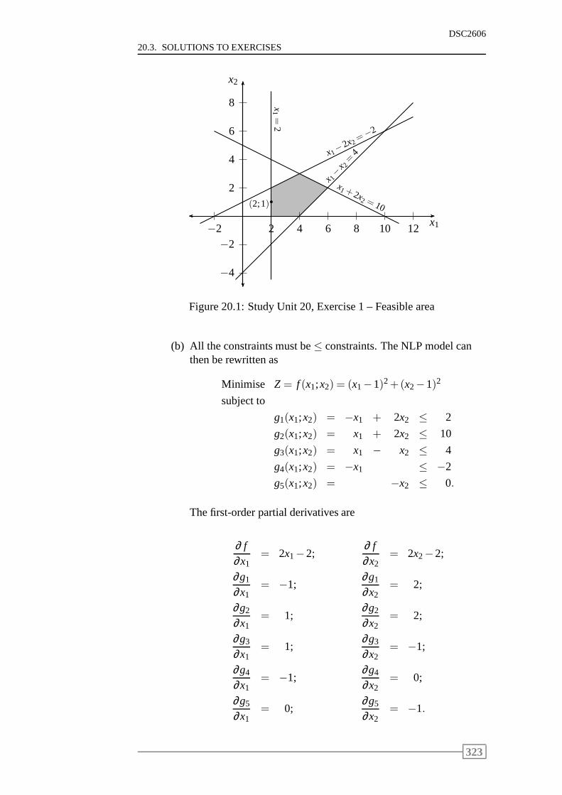
20.3. SOLUTIONS TO EXERCISES
DSC2606
2
4
6
8
−2
−4
2 4 6 8 10 12−2x1
x2
x1−2x2
=−2
x1 +2x2 = 10
x1− x2
=4
x1=
2
b(2;1)
Figure 20.1: Study Unit 20, Exercise 1 – Feasible area
(b) All the constraints must be≤ constraints. The NLP model canthen be rewritten as
Minimise Z = f (x1;x2) = (x1−1)2+(x2−1)2
subject to
g1(x1;x2) = −x1 + 2x2 ≤ 2
g2(x1;x2) = x1 + 2x2 ≤ 10
g3(x1;x2) = x1 − x2 ≤ 4
g4(x1;x2) = −x1 ≤ −2
g5(x1;x2) = −x2 ≤ 0.
The first-order partial derivatives are
∂ f∂x1
= 2x1−2;∂ f∂x2
= 2x2−2;
∂g1
∂x1= −1;
∂g1
∂x2= 2;
∂g2
∂x1= 1;
∂g2
∂x2= 2;
∂g3
∂x1= 1;
∂g3
∂x2= −1;
∂g4
∂x1= −1;
∂g4
∂x2= 0;
∂g5
∂x1= 0;
∂g5
∂x2= −1.
323
DSC2606
CHAPTER 20 KUHN-TUCKER CONDITIONS
The Kuhn-Tucker necessary conditions are
2x1−2−λ1+λ2+λ3−λ4+0λ5 = 0 (1)
2x2−2+2λ1+2λ2−λ3+0λ4−λ5 = 0 (2)
λ1(2+x1−2x2) = 0 (3)
λ2(10−x1−2x2) = 0 (4)
λ3(4−x1+x2) = 0 (5)
λ4(−2+x1) = 0 (6)
λ5(0+x2) = 0 (7)
λ1; λ2; λ3; λ4; λ5 ≥ 0.
Now substitute point(2;1) into the Kuhn-Tucker necessary con-ditions. Then we obtain the following:
Equation (7): λ5(1) = 0 ⇒ λ5 = 0.
Equation (6): λ4(−2+2) = 0 ⇒ λ4 > 0.
(This also follows from the fact that the fourth constraint is binding.)
Equation (5): λ3(4−2+1) = 0 ⇒ λ3 = 0.
Equation (4): λ2(10−2−2) = 0 ⇒ λ2 = 0.
Equation (3): λ1(2+2−2) = 0 ⇒ λ1 = 0.
Equation (2): 2−2= 0 ⇒ True.
Equation (1): 2(2)−2−λ4 = 0 ⇒ λ4 = 2.
Therefore, there are nonnegative multipliersλ1 = λ2 = λ3 = λ5 =0 andλ4 = 2 satisfying the Kuhn-Tucker necessary conditions atthe point(x1;x2) = (2;1).
Now we must verify whether the Kuhn-Tucker sufficient condi-tions are satisfied.
The second-order partial derivatives off (x1;x2) are
∂ 2 f
∂x21
= 2;∂ 2 f
∂x2∂x1= 0;
∂ 2 f
∂x22
= 2;∂ 2 f
∂x1∂x2= 0.
The Hessian matrix is
H(x1;x2) =
[
2 0
0 2
]
.
The first principal minors are 2 and 2; both positive. The sec-ond principal minor is 4, also positive. Therefore, the functionf (x1;x2) is a convex function.
324
20.3. SOLUTIONS TO EXERCISES
DSC2606
All five the constraints are linear. Therefore, the constraintsgi(x1;x2),i = 1; 2; 3; 4; 5, are convex functions.
This means that the Kuhn-Tucker sufficient conditions have beenmet.
We can conclude that(x1;x2) = (2;1) is the optimal solution tothe given NLP model.
325

DSC2606
CHAPTER 20 KUHN-TUCKER CONDITIONS
326