U.S. Department of Transportation

Federal Railroad Administration

Office of Research, Development and Technology

Washington, DC 20590

DOT/FRA/ORD-21/24 Final Report | August 2021

Categorizing Track Mud Spot Risk by Measurement of Vertical Track Deflection

i

NOTICE

This document is disseminated under the sponsorship of the Department of Transportation in the interest of information exchange. The United States Government assumes no liability for its contents or use thereof. Any opinions, findings and conclusions, or recommendations expressed in this material do not necessarily reflect the views or policies of the United States Government, nor does mention of trade names, commercial products, or organizations imply endorsement by the United States Government. The United States Government assumes no liability for the content or use of the material contained in this document.

NOTICE

The United States Government does not endorse products or manufacturers. Trade or manufacturers' names appear herein solely because they are considered essential to the objective of this report.

i

REPORT DOCUMENTATION PAGE Form Approved OMB No. 0704-0188

The public reporting burden for this collection of information is estimated to average 1 hour per response, including the time for reviewing instructions, searching existing data sources, gathering and maintaining the data needed, and completing and reviewing the collection of information. Send comments regarding this burden estimate or any other aspect of this collection of information, including suggestions for reducing the burden, to Department of Defense, Washington Headquarters Services, Directorate for Information Operations and Reports (0704-0188), 1215 Jefferson Davis Highway, Suite 1204, Arlington, VA 22202-4302. Respondents should be aware that notwithstanding any other provision of law, no person shall be subject to any penalty for failing to comply with a collection of information if it does not display a currently valid OMB control number. PLEASE DO NOT RETURN YOUR FORM TO THE ABOVE ADDRESS. 1. REPORT DATE (DD-MM-YYYY) August 2021

2. REPORT TYPE Technical Report

3. DATES COVERED (From - To)

June 2016–August 2020 4. TITLE AND SUBTITLE Categorizing Track Mud Spot Risk by Measurement of Vertical Track Deflection

5a. CONTRACT NUMBER DTFR5316C00016

5b. GRANT NUMBER

5c. PROGRAM ELEMENT NUMBER

6. AUTHOR(S) Christopher M. Hartsough 0000-0003-0320-3818

Joseph W. Palese 0000-0003-3946-3777

James P. Kelly 0000-0003-0207-011X

5d. PROJECT NUMBER

5e. TASK NUMBER Task # 1 & 2

5f. WORK UNIT NUMBER

7. PERFORMING ORGANIZATION NAME(S) AND ADDRESS(ES) Harsco Rail 1960 Old Cuthbert Road, Suite 100 Cherry Hill, NJ 08034

8. PERFORMING ORGANIZATION REPORT NUMBER

9. SPONSORING/MONITORING AGENCY NAME(S) AND ADDRESS(ES) U.S. Department of Transportation Federal Railroad Administration Office of Railroad Policy and Development Office of Research, Development and Technology Washington, DC 20590

10. SPONSOR/MONITOR'S ACRONYM(S)

11. SPONSOR/MONITOR'S REPORT NUMBER(S)

DOT/FRA/ORD-21/24

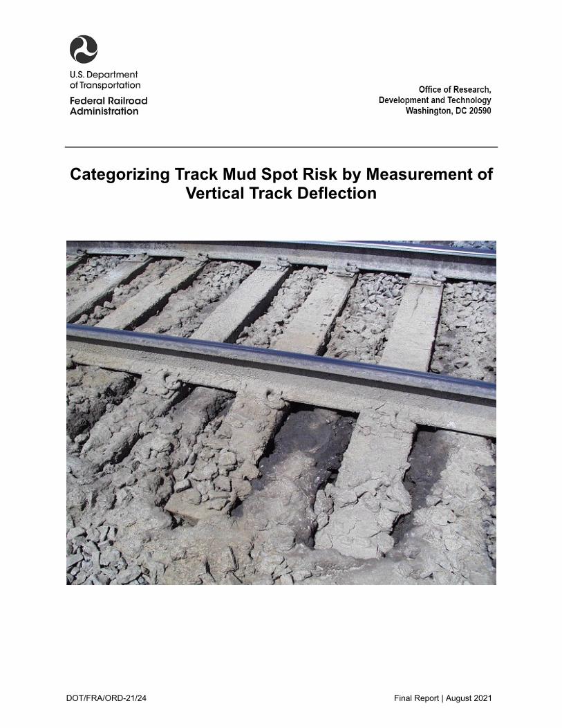
12. DISTRIBUTION/AVAILABILITY STATEMENT This document is available to the public through the FRA website. 13. SUPPLEMENTARY NOTES COR: Hugh Thompson 14. ABSTRACT Mud spots are a common problem faced by railroads where water, through capillary action, is “pumped” from the subgrade into the ballast by ties that move downward and upward under passing axle loads. When mud is mixed in with the ballast, several problems can occur which can increase the risk of derailment due to increased vertical track deflection. Maintenance crews typically know the location of their mud spots, and in general, perform repetitive, expensive, track time consuming maintenance to fix the symptom and not the root cause of the problem. If the level of risk for each mud spot were quantified, maintenance could be prioritized, whereby high-risk mud spots are addressed first, while low risk mud spots are monitored in the event their situation worsens. 15. SUBJECT TERMS Mud spot, vertical track deflection, risk, track maintenance, prioritization, track stiffness, Beam on Elastic Foundation, BOEF, MRail, YRel, radius of curvature, ballast, track, railroad 16. SECURITY CLASSIFICATION OF: 17. LIMITATION OF

ABSTRACT 18. NUMBER

OF PAGES 54

19a. NAME OF RESPONSIBLE PERSON a. REPORT b. ABSTRACT c. THIS PAGE

19b. TELEPHONE NUMBER (Include area code)

Standard Form 298 (Rev. 8/98) Prescribed by ANSI Std. Z39.18

ii

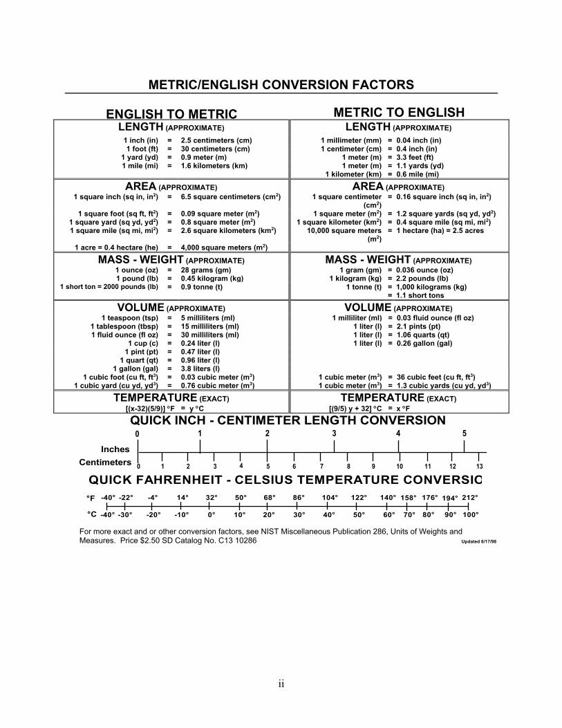
METRIC/ENGLISH CONVERSION FACTORS

ENGLISH TO METRIC METRIC TO ENGLISH

LENGTH (APPROXIMATE) LENGTH (APPROXIMATE) 1 inch (in) = 2.5 centimeters (cm) 1 millimeter (mm) = 0.04 inch (in) 1 foot (ft) = 30 centimeters (cm) 1 centimeter (cm) = 0.4 inch (in)

1 yard (yd) = 0.9 meter (m) 1 meter (m) = 3.3 feet (ft) 1 mile (mi) = 1.6 kilometers (km) 1 meter (m) = 1.1 yards (yd)

1 kilometer (km) = 0.6 mile (mi)

AREA (APPROXIMATE) AREA (APPROXIMATE) 1 square inch (sq in, in2) = 6.5 square centimeters (cm2) 1 square centimeter

(cm2) = 0.16 square inch (sq in, in2)

1 square foot (sq ft, ft2) = 0.09 square meter (m2) 1 square meter (m2) = 1.2 square yards (sq yd, yd2) 1 square yard (sq yd, yd2) = 0.8 square meter (m2) 1 square kilometer (km2) = 0.4 square mile (sq mi, mi2) 1 square mile (sq mi, mi2) = 2.6 square kilometers (km2) 10,000 square meters

(m2) = 1 hectare (ha) = 2.5 acres

1 acre = 0.4 hectare (he) = 4,000 square meters (m2)

MASS - WEIGHT (APPROXIMATE) MASS - WEIGHT (APPROXIMATE) 1 ounce (oz) = 28 grams (gm) 1 gram (gm) = 0.036 ounce (oz) 1 pound (lb) = 0.45 kilogram (kg) 1 kilogram (kg) = 2.2 pounds (lb)

1 short ton = 2000 pounds (lb) = 0.9 tonne (t) 1 tonne (t)

= =

1,000 kilograms (kg) 1.1 short tons

VOLUME (APPROXIMATE) VOLUME (APPROXIMATE) 1 teaspoon (tsp) = 5 milliliters (ml) 1 milliliter (ml) = 0.03 fluid ounce (fl oz)

1 tablespoon (tbsp) = 15 milliliters (ml) 1 liter (l) = 2.1 pints (pt) 1 fluid ounce (fl oz) = 30 milliliters (ml) 1 liter (l) = 1.06 quarts (qt)

1 cup (c) = 0.24 liter (l) 1 liter (l) = 0.26 gallon (gal) 1 pint (pt) = 0.47 liter (l)

1 quart (qt) = 0.96 liter (l) 1 gallon (gal) = 3.8 liters (l)

1 cubic foot (cu ft, ft3) = 0.03 cubic meter (m3) 1 cubic meter (m3) = 36 cubic feet (cu ft, ft3) 1 cubic yard (cu yd, yd3) = 0.76 cubic meter (m3) 1 cubic meter (m3) = 1.3 cubic yards (cu yd, yd3)

TEMPERATURE (EXACT) TEMPERATURE (EXACT) [(x-32)(5/9)] °F = y °C [(9/5) y + 32] °C = x °F

QUICK INCH - CENTIMETER LENGTH CONVERSION10 2 3 4 5

InchesCentimeters 0 1 3 4 52 6 1110987 1312

QUICK FAHRENHEIT - CELSIUS TEMPERATURE CONVERSIO -40° -22° -4° 14° 32° 50° 68° 86° 104° 122° 140° 158° 176° 194° 212°

°F

°C -40° -30° -20° -10° 0° 10° 20° 30° 40° 50° 60° 70° 80° 90° 100°

For more exact and or other conversion factors, see NIST Miscellaneous Publication 286, Units of Weights and Measures. Price $2.50 SD Catalog No. C13 10286 Updated 6/17/98

iii

Acknowledgements

This effort would not have been possible without the support of CSX, Conrail, and MRS Logística (Brazil) railways and their engineering staff, who graciously provided motive power, track time, and data. Their help and cooperation are greatly appreciated.

iv

Contents

Executive Summary ........................................................................................................................ 1

1. Introduction ................................................................................................................. 3 1.1 Background ................................................................................................................. 3 1.2 Objectives .................................................................................................................... 4 1.3 Overall Approach ........................................................................................................ 4 1.4 Scope ........................................................................................................................... 6 1.5 Organization of the Report .......................................................................................... 6

2. Data Collection and Preliminary Analysis .................................................................. 7 2.1 Data Acquisition .......................................................................................................... 7 2.2 Report Generation ..................................................................................................... 11

3. Development of Risk Guideline ................................................................................ 15 3.1 Beam on Elastic Foundation ...................................................................................... 15 3.2 YRel from BOEF ....................................................................................................... 20 3.3 YRel Signature at Soft/Mud Spot .............................................................................. 20 3.4 Geometric Risk Guideline ......................................................................................... 24 3.5 Time Component for the Risk Guideline .................................................................. 28

4. Application of Risk Guideline ................................................................................... 33 4.1 Soft/Mud Spot Identification ..................................................................................... 33 4.2 Sample Geometric Risk Guideline Application ........................................................ 36 4.3 Sample Geometric Risk Guideline Application with Time Component ................... 38

5. Future Activities ........................................................................................................ 41

6. Conclusion ................................................................................................................. 42

7. References ................................................................................................................. 43

Abbreviations and Acronyms ....................................................................................................... 44

v

Illustrations

Figure 1. Typical mud spot ............................................................................................................. 3

Figure 2. MRail vertical track deflection measurement system ..................................................... 5

Figure 3. MRail system mounting brackets mounted on revenue car ............................................. 5

Figure 4. System map with inspection route designations .............................................................. 8

Figure 5. MRS instrumented ore car ............................................................................................... 9

Figure 6. MRail system GPS traces during various inspections (axes represent GPS coordinates)............................................................................................................................................... 11

Figure 7. Example strip chart reports ............................................................................................ 13

Figure 8. Sample CSV exception report with GPS excluded ....................................................... 14

Figure 9. BOEF model .................................................................................................................. 15

Figure 10. Plot of BOEF deflection (w(x)) with MRail measurement for multiple wheel loads .. 16

Figure 11. Stiffness model of soft spot in track subjected to two wheel loads (one truck/bogie) 18

Figure 12. Deflection “plot” for a two-wheel bogie with varying soft spot track modulus ......... 19

Figure 13. Deflection “map” (maximum deflection) for a bogie varying with soft spot track modulus ................................................................................................................................. 19

Figure 14. BOEF rail deflection and YRel ................................................................................... 20

Figure 15. Location of YRel exception ......................................................................................... 21

Figure 16. Satellite image of exceedance ..................................................................................... 22

Figure 17. Expanded view of left rail YRel at exception (soft/mud spot) .................................... 22

Figure 18. Overlay of left rail YRel and BOEF model (blue: YRel, orange: BOEF model) ....... 23

Figure 19. YRel versus bending stress .......................................................................................... 25

Figure 20. Radius of curvature of the deflected rail versus stress ................................................ 26

Figure 21. Risk parameters from measured data .......................................................................... 27

Figure 22. Radius of curvature based on mud spot length and central deflection change from the peak uplift vs. specific radius of curvature values ................................................................ 28

Figure 23. KM 257 for multiple inspection runs .......................................................................... 29

Figure 24. Mud spot approximately at KM 257.35 for multiple inspections ............................... 30

Figure 25. Overlaid and aligned YRel left data in vicinity of mud spot (KM 257.35) ................. 31

Figure 26. Risk and peak deflection values over time for two mud spot locations ...................... 32

Figure 27. FFT of YRel data ......................................................................................................... 34

Figure 28. Sample mud spot YRel (top/a) and first difference of YRel (bottom/b) ..................... 35

Figure 29. 0.6 miles (1.0 km) of potential mud spots for a plot of left rail YRel data ................. 35

vi

Figure 30. Distribution of identified full signal widths ................................................................ 36

Figure 31. Risk (radius of curvature (r)) of identified mud spot signatures plotted against rail based flexural stress thresholds ............................................................................................. 37

Figure 32. Histogram of radius of curvature (Risk (r)) of flagged signals by thresholds ............. 37

Figure 33. Risk (r) values for 3 miles of soft/mud spots for seven inspections ............................ 39

Figure 34. Plot of mean inspection session mud spot Risk (r) for the 3 miles inspection location (six inspections) .................................................................................................................... 39

vii

Tables

Table 1. Current first level risk concept .......................................................................................... 1

Table 2. Summary of data acquisition ............................................................................................ 7

Table 3. MRS inspection route designations .................................................................................. 9

Table 4. MRS measurement campaign ......................................................................................... 10

Table 5. Car characteristics for BOEF plot ................................................................................... 17

Table 6. Radius of curvature and intermediate calculations ......................................................... 25

Table 7. Risk assessment of mud spot .......................................................................................... 32

Table 8. Three miles of mud spots for seven inspections ............................................................. 38

1

Executive Summary

This report presents the concluding results related to Phase 1 of the Federal Railroad Administration’s (FRA) Broad Agency Announcement (BAA) project Categorizing Track Mud Spot Risk by Measurement of Vertical Track Deflection. The overall goal of the project was to develop a means of using vertical track deflection measurement data to determine a risk value associated with a given mud spot in track, based on current vertical track deflection measurement capability. This in turn can then be used for prioritizing maintenance of identified mud spots. Specifically, for Phase 1 of the project, Harsco Rail’s goal was to both collect vertical track deflection measurement data and to use that data to develop an initial model framework, with a first order application from June 2016 through August 2020. Researchers used the MRail system to collect vertical track deflection data. This system consists of both an optical laser/camera sensor head and control hardware for managing and processing the sensor head data into vertical track deflection values captured every foot. MRail systems were deployed to two heavy haul railroads—one in the United States (CSX) and one in Brazil (MRS Logística)—for vertical track defect data collection. Using the collected data, a mud spot risk model was created based on Beam on Elastic Foundation (BOEF) theory and the American Railway Engineering and Maintenance-of-Way (AREMA) rail base allowable flexural stress. In general, soft/mud spots result in a differential peak deflection when a train passes over it. Thus, the radius of curvature of the deflected rail shape will vary based on the support stiffness in the parent track and the support stiffness and the length of the mud spot. Since support stiffness is directly relatable to the vertical track deflection measured by the MRail system, a risk model based on associating a soft/mud spot’s radius of curvature was created to accommodate the varying features of each soft/mud spot. This was achieved by analyzing the MRail deflection signature to identify the length of the location in track and its peak deflection difference. These parameters were then used to determine the radius of curvature of the deflected rail and associated risk value. As radius of curvature decreases, rail flexural stress in the base increases. Using the AREMA rail base flexural stress limit of 25,000 psi, conservative initial thresholds based on a rail’s radius of curvature were created. The 25,000-psi limit would be reached in the base of a rail which is experiencing a radius of curvature of approximately 325 ft. The current first level risk concept, which provides a factor of safety to allow for remedial action, is shown in Table 1.

Table 1. Current first level risk concept

Radius of Curvature (ft) Risk Level Action r > 2,000 ft Low None

500 ft < r < 2,000 ft Moderate Monitor r < 500 ft High Remedial Action

As a proof of concept, the developed methodology was applied to approximately 850 miles of track identified in the collected test data. The research team developed an automated method for analyzing the deflection signal while utilizing the Fast Fourier Transform (FFT). This method allows for automatically identifying soft spots in track, though field verification of the presence of mud associated with this soft spot is required at this time. Approximately 500 soft spots, mud spot like signatures, were identified in the 850 miles of track data analyzed.

2

Each signature was then processed to generate its associated risk (r) value expressed as its radius of curvature of the deflected rail shape. The application of this methodology showed that 150 of the locations (30%) had a radius of curvature less than 500 ft, 220 locations (44%) had a radius of curvature between 500 and 2,000 ft, and the remainder (26%) had a radius if curvature greater than 2,000 feet. Thus, considering the conservative nature of the approach, 150 locations require field verification, and their associated risk value (i.e., radius of curvature, where lower values imply higher risk) can be used to prioritize remedial action. Under Phase 2 of this research activity, the methodology developed will be applied to a designated test track which is regularly measured by an MRail system. Through coordination with local maintenance personnel and correlation with track level inspection data, the model will be refined to increase usability for prioritizing mud spot maintenance.

3

1. Introduction

The Federal Railroad Administration’s Broad Agency Announcement (BAA) project funded this research effort to classify mud spot1 conditions with its impact on track maintenance, and more importantly its potential for track safety improvement. With all the sophisticated highly technical track measurement systems that have been developed over the last two decades, there is still no definite measurable method to objectively value the safety risk of track mud spots. The technology exists to do this, but it has not been applied specifically for this purpose. Since the technology to measure vertical track deflection under heavy axle load already exists, this is not a research project for the development of vertical track deflection measurement, rather it is a development project for quantifying risk. The mission of the project is to demonstrate that evaluation, classification, and risk assessment of mud spots is feasible, practical, and low in cost for a large improvement in track—train operating safety.

1.1 Background A significant number of mud spots exist on approximately 160,000 miles of track in use today in the USA. Mud spots are a very common problem where water, through capillary action, is “pumped” from the subgrade into the ballast by ties that move up and down under axle loads passed over the tie. The tie acts like a piston pump as the rail elasticity springs the tie upward after the axle load passes over the tie. Consider a train with 100 cars and 4 axles per car. With this consist, each tie moves down and then back up 400 times for the passage of 1 train. With a wet subgrade, water and mud are drawn into the ballast by the pumping of these ties. Figure 1 shows the results of repeated axles passing over a significant mud spot.

Figure 1. Typical mud spot

1 The definition of a mud spot is a location in track of defined length where capillary action from repeated wheel loading (“pumping”) draws finer soil granules from the subgrade up into the ballast causing contamination, known as fouling. The presence of water exacerbates this phenomenon and mud appears on the track/tie surface.

4

Mud (i.e., wet soil particles) mixed in with the ballast (i.e., known as ballast fouling) causes several problems that increase derailment risk, this includes:

• Less stable muddy ballast

• Significant vertical track deflection

• Increased rail stresses due to unintended additional flexure of the rail under load

• Areas where timber ties rot quickly

• Poor track gage holding stability due to rotting ties (e.g., reduced later track strength)

• Weakened lateral resistance for track alignment

• Higher risk of track buckling (e.g., sun kinks) under increased compressive thermal stresses, and poor track running surface

The most significant problem with mud spots is that there are usually too many on the property for any railroad to immediately address. In addition, the severity of a mud spot is not easily defined (i.e., often defined subjectively) and correction requires invasive maintenance activities with significant track disruption. The most typical remedial action, tamping, tends to only address the symptom and not the root cause of the mud spot. This drives a need to have a low cost and fast way to evaluate the risk of each mud spot and help prioritize maintenance.

Field personnel generally know where mud spots are located on their territory, and in general, perform repetitive maintenance to fix the symptom and not the root cause of the problem. This maintenance is expensive and requires track time. If the level of risk for each mud spot were quantified, maintenance could be prioritized. It would then be practical to repair the high-risk mud spots while keeping a close watch on the low risk mud spots in case their situation worsens. In this manner, remedial actions can be identified and planned for various levels of maintenance and corrective action.

1.2 Objectives The overall objective of this project is to generate a means of associating a risk value to a mud spot identified in track using an automated means of measuring vertical track deflection. The resultant risk values would allow maintenance departments the ability to prioritize time and resources (e.g., capital, crews, materials, etc.) to track locations that require more urgent repairs.

1.3 Overall Approach The method to quantify the level of risk of each mud spot is to analyze near continuous vertical track deflection data from the MRail Vertical Track Deflection System in conjunction with other railway track and operating data. The MRail system (Figure 2) is installed on a fully loaded freight car (Figure 3) such as a coal car, hopper car, or other car that can be easily loaded to near maximum allowable axle load. The MRail Vertical Track Deflection System has been extensively tested and provides valuable data. The system uses machine vision (e.g., lasers/cameras) to make a chord-based measurement of deflection away from the truck/bogie, utilizing the truck/bogie frame as a chord reference. The MRail equipped car can be coupled into a normal local or through freight train just as any other revenue car to collect data autonomously.

5

Figure 2. MRail vertical track deflection measurement system

Figure 3. MRail system mounting brackets mounted on revenue car

For this project (i.e., specifically Phase 1 which is discussed in this report), an MRail equipped car traversed specific lines of track on several railways that operate heavy axle loads, with close coordination with the local field personnel. Vertical track deflection data was collected and transmitted to Harsco Rail for analysis. The data included the continuous vertical track deflection data that could be correlated with each mud spot (or suspected mud spot) for further analysis. An important factor in this project was to measure vertical track deflection for the same locations over time and changes in weather to determine the trend. For example, a mud spot that has a 1.5-inch vertical deflection would require immediate attention, but a mud spot with 0.5 inches of deflection may be monitored over time and traffic to determine the trend. With this method and for the first time, the railroad will be able to assign a very meaningful number to the condition of each mud spot. This will include the current condition as well as rate of failure. Building on that basic assessment, a risk assessment model was developed for use on mud spots that considers not only the measured vertical track deflection, but also the track’s specific operating conditions (i.e., type of traffic, speed, etc.) as it relates to the bending stress present in the rail. With the developed risk assessment model, railroads can correct the high-risk mud spots

6

and monitor the trend of the remaining mud spots over time and traffic. Overall, the track will be much safer since the limited resources to repair mud spots will be prioritized and not be wasted on locations that do not need immediate attention.

1.4 Scope This document and its contents are limited to Phase 1 of a two-phase project. Phase 1 encompassed large-scale vertical track deflection measurement data collection, preliminary mud spot risk model development, and initial applications of the risk model. The risk model presented in this report is not yet in its finalized form as continued refinement is expected to occur during Phase 2 of this project. Phase 2 will include additional vertical track deflection data collection, risk model refinement based on correlation to actual mud spots, and risk model refinement based on partner railroad feedback.

1.5 Organization of the Report Section 2 details the data collection conducted with different partner railroads as well as explanations of the output generated by the data collection system (MRail). Section 3 explores how the initial mud spot risk model was developed. This includes comparisons of vertical track deflection data to fundamental beam on elastic foundation (BOEF), the basis used for risk determination, and the generated risk model itself. Section 4 shows a typical application of the mud spot risk model on actual vertical track deflection data. Sections 5 and 6 discuss concluding results and recommendations for future work.

7

2. Data Collection and Preliminary Analysis

To properly develop the risk guidelines (i.e., the main output of this project), vertical track deflection data was required. Collecting this data involved deploying the MRail system to a railroad to gather large amounts of data over locations which contained mud spots.

2.1 Data Acquisition As part of this study, MRail vertical track deflection data was collected on two railways due to some reliability issues with the MRail system, and the inability to make repeated measurements. Table 2 summarizes the data collection activities and amount of data collected.

Table 2. Summary of data acquisition

Railway Date Range Route Length Cycles Total

Length Partner

CSX Sept. 2016 to Feb. 2017 N/A N/A 5,000 mi Cost shared inspection

MRS Logística (Brazil)

Feb. 2017 to Jul. 2018 450 mi 10 4,500 mi Donated data

Researchers collected data on CSX by putting the MRail measurement car into the track geometry consist for 6 months, which is the timeframe that CSX committed to. Thus, data collection was limited to the locations traversed based on the geometry car schedule. During the data collection activity on CSX, the data acquisition system experienced reliability issues. These issues included damage to the sensor heads from prolonged use (e.g., lens contamination, moisture infiltrations, and broken coverings), loss of light shielding causing sun infiltration, and a system virus through the unprotected modem. Ultimately, approximately 5,000 miles of vertical track deflection data was collected. In parallel with attempting to collect more data locally in the United States, another MRail system was deployed to MRS Logística in Brazil under a separate project. MRS Logística S.A. (Malha Regional Sudeste) is a heavy haul freight railway in Brazil which operates over 1,000 miles of track throughout south eastern Brazil. Figure 4 shows a system map with inspection route designation. Table 3 shows the boundaries of the MRS defined inspection routes.

8

Figure 4. System map with inspection route designations

9

Table 3. MRS inspection route designations

The MRail system was installed on an instrumented ore car (Figure 5) and placed in a revenue train consist. This car was used from February 2017 to July 2018 to collect vertical track deflection measurement data from over 4,500 miles of track. Table 4 shows locations and dates of data collection activities.

Figure 5. MRS instrumented ore car

Location KM Line Location KM Line1 Ferrovia do Aço P1-07 292.989 L2 Ferrovia do Aço P2-14 3.787 L12 Saudade-Barra Saudade 156.473 L2 Saudade-Barra Barra do Piraí 108.222 L13 Saudade-Barra Barra do Piraí 108.222 L1 Barra - Brisamar Posto KM 30 30.000 S/Inf4 Barra - Brisamar Brisamar 27.120 - Barra - Brisamar Barra do Piraí 108.222 L1

Linha do Centro Aristides Lobo 113.000 L1 Linha do Centro Caetano Lopes 498.550 L1Ferrovia do Aço P1-06 306.806 L1 Ferrovia do Aço P1-03A 349.728 L1

5 Brisamar - Saí Saí 4.438 L1 Brisamar - Saí Itacuruçá 16.985 L17 Paraopeba Jeceaba 504.180 L1 Paraopeba Eng. Pedro Paulo 606.571 L19 Ferrovia do Aço P1-06 306.806 L1 Ferrovia do Aço P1-03 (Andaime) 353.666 -10 Ferrovia do Aço P1-03 (Andaime) 353.666 - Ferrovia do Aço P1-05A 318.599 L111 Paraopeba Ibirité 612.735 L4 Paraopeba Jeceaba 504.180 L112 Paraopeba Olhos D'Água 623.853 S/Inf Paraopeba Olhos D'Água 612.375 S/Inf

TrackEnd

Route TrackStart

10

Table 4. MRS measurement campaign Run Route Season Start Finish Comments 1

1 1,2,3,4,5,4,3,6,7,1 Dry 7/19/2017 7/22/2017 Reported measurements problems between 4 to 6

2 1,2,3,4,3,6,7,8,9,10,9,8,1 Dry 7/24/2017 7/26/2017 Reported camera problems between 4 to 6

3A 1,7,8,9,10,9,8,7,8,11,8,7,1 Dry 7/31/2017 8/2/2017

3B 1,2,3,4,3,6,7,1 Dry 8/2/2017 8/4/2017

4 8,9,10,9,8,7,8,11,12,11,8,7,1,2,3,4,5,4,3,6,7 In between 9/12/2017 9/15/2017 Reported measurements problems between 4 to 6

Bridge 1 – AB In between 10/10/2017 10/10/2017 Bridge location KM 097 + 327

5 Bridge 2 – CD In between 10/24/2017 10/24/2017 Bridge location KM 19 + 795

Bridge 1 - AB In between 12/5/2017 12/5/2017 Bridge location KM 097+327 – GPS problem reported

6 4,3,6,7,8,9,10,9,8,7,8,11,12,11,8,7,1,2,3,4 Wet 11/20/2017 11/24/2017 GPS problem reported

7 4,5,4,3,6,7,8,9,10,9,8,7,8,11,12,11,8,7,1,2,3,4 Wet 11/28/2017 12/2/2017 GPS problem reported

8 1,2,3,4,5,4,3,6,7,8,9,10,9,8,7,8,11,12,11,8,7,1 Wet 2/21/2018 2/25/2018 GPS problem reported

9 1,2,3,4,5,4,3,6,7,1 Wet 2/28/2018 3/4/2018

10 1,2,3,4,3,6,7,1 Wet 3/9/2018 3/15/2018

11 1,2,3,4,5,4,3,6,7,8,9,10,9,8,7,8,11,12,11,8,7,1 Dry 6/28/2018 7/5/2018

12 1,2,3,4,3,6,7,1 Dry 7/7/2018 7/11/2018

13 1,2,3,4,3,6,7,1 Dry 7/13/2018 7/18/2018

Vertical track deflection data was primarily collected from a 450-mile route which was repeatedly measured. Figure 6 shows a plot of the Global Positioning System (GPS) coordinates collected during three separate inspection runs, i.e., the plot shows where data was collected. It can be seen from this figure that not all the track had data successfully collected during all three runs (i.e., right hand portion of plot). However, coverage of a substantial portion of the track resulted in sufficient data for comparison purposes. Approximately 10 inspections were conducted over 3 separate seasonal time periods (see Table 4). Brazil experiences a rainy and dry season that directly affects the track response. Thus, measurements were taken during these seasons, with additional runs in between these seasons, to identify track response differences. MRS kindly donated their data to aid in the research effort performed herein to allow for additional verification as well as implementation of a time dependent component to the risk guideline. Note that the comprehensive risk guideline—and resulting maintenance strategy—is intended to be validated on a US freight railway using the FRA MRail (i.e., on the DOTX218 car) system and/or Harsco MRail system (i.e., on Harsco’s inspection car). Fundamentally, both the DOTX218 and Harsco inspection car MRail system are the same. The primary difference is that the DOTX218 system is configured and calibrated to function on a car with a secondary suspension while the Harsco inspection car system is not.

11

Figure 6. MRail system GPS traces during various inspections (axes represent GPS

coordinates) During data acquisition, the raw image data is transformed and saved for offline processing. During the offline processing the following occurs:

• Calculate YRel (i.e., relative deflection value) for each rail from the raw image signals

• Align GPS coordinates to railway milepost (MP) designations using mapping file

2.2 Report Generation For all the data collected, base reports were created that included the following:

• Strip chart (1 mile per page) o Location identification information (top horizontal banner) Railroad route identifiers Date of inspection Report MP range

o MP range for page (right vertical banner) o Date of report and page number of number of pages (bottom horizontal banner) o Measured data (top (left rail) and bottom (right rail) plot windows) Foot-by-foot data plots2

• YRel (inches)

2 Note that the vertical scales are inferred by the marked threshold lines

12

• YRel roughness (square inches)3 o One-mile summary statistics for each rail (to the left of data plot windows) Mathematical average of YRel for the mile Maximum value of YRel for the mile, actual value inclusive of all track type (e.g.,

switches, crossing, bridges, etc.) Percentage of “Smooth” rail

• Percentage of measurements below the “Acceptable” YRel threshold

• Lowest data bucket which indicates nominal support performance Percentage of “Acceptable” rail

• Percentage of measurements below the Yellow YRel threshold

• Second lowest threshold which indicates YRel measurements are above nominal and approaching the yellow limit

Percentage of “Yellow” rail

• Percentage of measurements above a YRel Yellow threshold but below the Red

Percentage of “Red” rail

• Percentage of measurements above a YRel Red threshold Number of Yellow exceptions; number of measurements above a YRel Yellow

threshold Number of Red exceptions; number of measurements above a YRel Red threshold

o Heat map of YRel measurements (central plot window) Color coding of YRel measurements; blue is zero and red is above the Red

threshold, with color gradient in between Includes location marks for Red and Yellow exceedances

• Exception report (1 mile per page) o Include YRel plots per the above definitions o List of locations that exceed a pre-defined threshold Red Level (safety) Yellow Level (maintenance)

o GPS coordinates of exception o Includes maximum value in consecutive measurements exceeding threshold

3 Roughness is defined as a mean square statistic as follows:

13

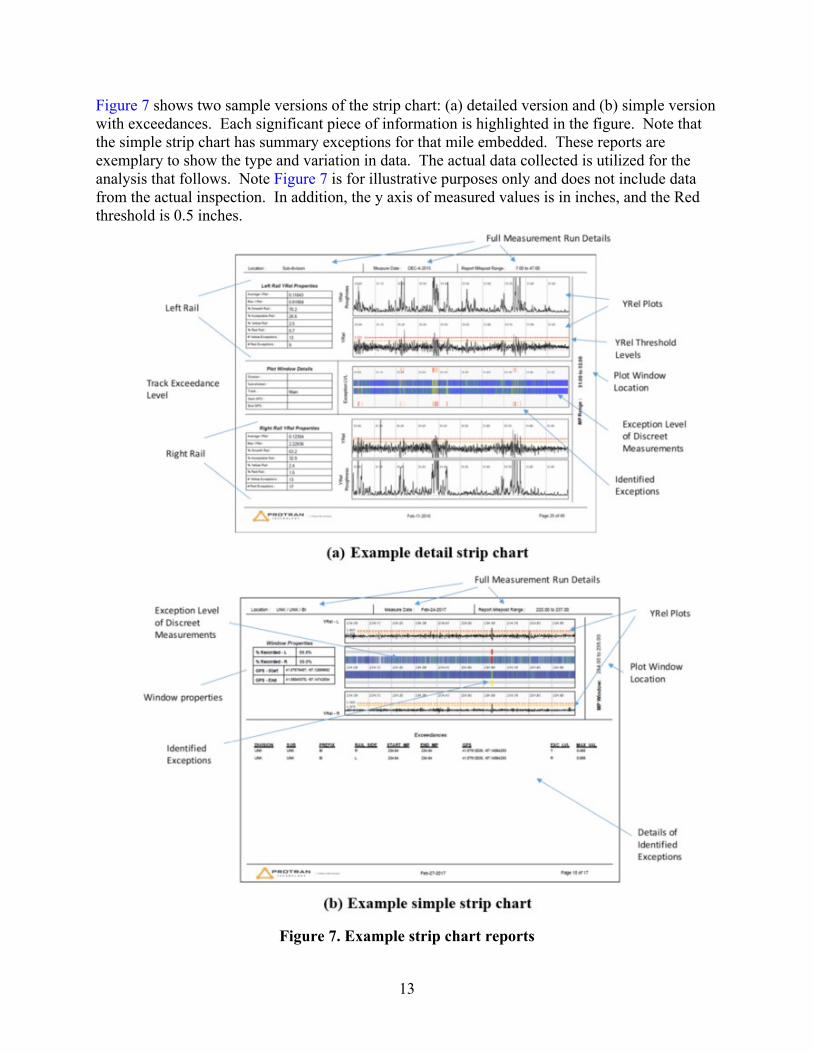
Figure 7 shows two sample versions of the strip chart: (a) detailed version and (b) simple version with exceedances. Each significant piece of information is highlighted in the figure. Note that the simple strip chart has summary exceptions for that mile embedded. These reports are exemplary to show the type and variation in data. The actual data collected is utilized for the analysis that follows. Note Figure 7 is for illustrative purposes only and does not include data from the actual inspection. In addition, the y axis of measured values is in inches, and the Red threshold is 0.5 inches.

Figure 7. Example strip chart reports

14

The graphical data described above is complimented by text output files to be used for further analysis in a Comma Separated Value (CSV)4 format. The exception report (see example records shown in Figure 8) is a list of locations that exceed user define thresholds. For each exception, the bounding location is identified (e.g., railroad location identifiers, KM/MP limits, and rail side), along with its classification (e.g., EX_LVL = ‘Y’ for Yellow exception, and ‘R’ for Red exception), along with its maximum exceedance value within in the sequence of measurements that exceed the threshold. It should be noted that the exception thresholds (Red and Yellow) are user/railroad defined, whereby Red indicates a safety exception, and Yellow indicates a maintenance exception. These values can vary based on line speed, cargo carried, and any other number of factors. The study herein used the YRel measurements themselves.

Figure 8. Sample CSV exception report with GPS excluded

4 CSV and is a standard format for importing text data into other software for analysis purposes.

15

3. Development of Risk Guideline

Vertical track deflection data provides valuable insight into the support stiffness of the track as shown in Section 2. In addition to average support stiffness, soft spots in track are easily identified. Of particular interest is the condition of mud spots and how this condition changes over time. Over long stretches, the average YRel value gives a good indication of the average track stiffness (or modulus) for that section of track, i.e., the mean in a window of track of 500 ft will provide valuable insight into the track support modulus. This is an important parameter used in BOEF analysis for understanding the distribution of stresses through the track components. However, localized, significant variation in vertical track deflection—variation in YRel—are indicative of an abrupt change in track stiffness. Various track deflection signatures can be related to stiffness variations in track, i.e., soft spot, mud spot, stiff spot, stiffness transitions at grade crossings and bridges, etc.

3.1 Beam on Elastic Foundation MRail measures relative deflection of the top of rail under moving load. As such, it offers the ability to estimate track modulus of the underlying substructure. Track modulus can be defined as the linear elastic support stiffness for a beam (rail) continuously supported by an elastic foundation (BOEF). BOEF theory has several assumptions and shortfalls. However, BOEF remains the predominant theory used in track component design and stress analysis. Figure 9 below shows the BOEF model.

Figure 9. BOEF model

The defining differential equation and solution for deflection for a standard BOEF model under a point load (single wheel) is shown below:

(1)

(2)

16

Where w(x) = rail deflection at location x P = wheel load k = track modulus or stiffness E = rail modulus of elasticity I = rail moment of inertia And introducing parameter β with units 1/length, where

This solution can be applied for multiple wheels using linear superposition and summing solutions. This is required when analyzing the MRail data as adjacent wheels influence overall deflection of the rail, and the YRel results. When considering the solution algorithm above for multiple wheels, Figure 10 shows a typical deflection plot for uniform track modulus for track and vehicle characteristics defined in Table 5. Note that the individual wheel deflections are summed, using the principles of linear superposition, for the overall track deflection for two cars coupled. This is a static representation with the car generally coupled at the end of the train, and the train moving from right to left.

Figure 10. Plot of BOEF deflection (w(x)) with MRail measurement for multiple wheel

loads

-0.250

-0.200

-0.150

-0.100

-0.050

0.000

0.050

-250 -50 150 350 550 750 950 1150

Defle

ctio

n, w

(in)

Distance from lead wheel (in)

Deflection - All Wheels

Mrail Reference

YRel

All other lines are individual wheel deflections

1 2 876543

17

Table 5. Car characteristics for BOEF plot

Freight Car Car Type Wheel Cumulative

Wheels

Dist from Adjacent

Wheel x

(inches) x (feet)

317,467 lbs

4

39,683 lbs Car 1 1 1 0 0 0.0

45 mph 2 2 72 72 6.0

36 inches 3 3 176 248 20.7

56,053 lbs 4 4 72 320 26.7

413 inches Car 2 1 5 165 485 40.4

248 inches 2 6 72 557 46.4

72 inches 3 7 176 733 61.1

176 inches 4 8 72 805 67.1

Car Weight

Axles

Ps

V

D

Pd

Len Over Couplers

Truck Spacing

Axle Spacing

Len Bet Inner Whls

Len Outer Whl to Coup 82.5 inches

In Table 5, the following are defined and explained, and relate to Figure 10:

• Ps is the static wheel load; car weight divided by eight wheels

• V is the speed of the train

• D is the wheel diameter

• Pd is the dynamic wheel load based on the AREMA formula

o

• The remaining variables describe the longitudinal geometry of the train consist and allowfor determination of spacing of wheel loads as shown in Figure 10o The right three columns in Table 5 show the buildup of the wheel spacing, including: Distance between adjacent wheels Cumulative distance from wheel 1 in inches Cumulative distance from wheel 1 in feet

The solid Red line in Figure 10 depicts the MRail system reference chord, and the dashed Red line is the resulting YRel measurement from the measurement consist. This figure shows the deflection “plot” for a time slice of the train on the track, at a specific location, i.e., how the rail would deflect along the track’s longitudinal axis from the adjacent wheels of two cars. As the train moves down the track, this deflection “plot” moves as well—and may vary as a function of support stiffness variations—and the YRel measurement captured for each point along the track is the peak deflection at that point in track. The point captured by MRail for each time slice (i.e., approximately 1.09 ft of train travel) defines the deflection “map,” or maximum value at that time slice and corresponding location on the track. Thus, it is extremely important to note that

18

for uniform support stiffness, applied load and constant rail section, the resulting deflection “map” (i.e., measured YRel at each point along the track) would be a constant value. In reality, the support stiffness is not constant. In fact, the load may have a dynamic augment, and the rail section could change (or be worn). Thus, a typical YRel plot shows the deflection “map” (as shown previously in Figure 7a). Note the variation in YRel, which clearly shows that the support stiffness is not uniform (the load and rail section properties may vary as well). Note the spikes5 in YRel which correspond to localized soft spots. These soft spots may or may not be actual mud spots and must be field verified at this time. However, all soft spots represent abrupt changes in the track support stiffness which may indicate superstructure issues (e.g., soft joint, failed ties/fasteners, etc.), or substructure performance issues (e.g., mud spots, hanging ties, etc.). In fact, soft spots may display a particular signature in the YRel data. This will be discussed later in this section. An example of a model for a uniform soft spot in track (e.g., mud spot, kmud), surrounded by uniform stiffness (e.g., parent track, kparent) can be defined as shown in Figure 11. This results in a much more complex mathematical model (i.e., three differential equations with matching and boundary conditions) that can be solved and applied.

Figure 11. Stiffness model of soft spot in track subjected to two wheel loads (one

truck/bogie) The solution of the model presented above for different values of stiffness in the soft spot (500, 1,500, and 2,500 lb/in/in) and a constant parent track/surrounding stiffness (3,500 lb/in/in) are shown in Figure 12. This figure shows the deflection of the rail at the center of the soft spot. The deflection basin can be seen to dissipate away from the load as expected. As the soft spot gets softer, the deflection basin deepens and widens. Note that the blue line is for equal soft and parent track stiffness values (3,500 lb/in/in). The blue shaded area is the location and extent of the softer track. This is referred to as the deflection “plot” and represents the defection of the rail at a snapshot in time, at the center of the soft spot, as the wheel passes over the track.

5 The definition of spikes in this context are values which noticeably deviate from the average oscillatory YRel signal.

kparentkparentkmud

19

Figure 12. Deflection “plot” for a two-wheel bogie with varying soft spot track modulus

Considering the deflection “map” (i.e., peak deflection as the train moves down the track),6 Figure 13 shows the maximum deflection at each point along the track for several values of soft track stiffness. Note that when soft and parent track stiffness values are equal (i.e., the blue line), the maximum deflection is constant along the track (i.e., 0.2 inches). Also, as the train approaches the softer support stiffness, deflection starts to increase outside of the soft stiffness zone (i.e., blue shaded area) since the deflection is influenced by the surrounding stiffness values, and the bending stiffness of the rail.

Figure 13. Deflection “map” (maximum deflection) for a bogie varying with soft spot track

modulus

6 Note that this is a quasi-static analysis that is symmetric, and the direction of train travel is not relevant. In addition, this analysis does not assume any lateral loading, and it is assumed that the car weight is equally distributed on all eight wheels. Thus, the results are representative of tangent track.

-0.2

0.0

0.2

0.4

0.6

0.8

1.0

1.2

0 20 40 60 80 100

w (i

n)

Location (ft)

2-Wheel Deflection

3500 2500 1500 500k (lb/in/in) =

0.0

0.2

0.4

0.6

0.8

1.0

1.2

20 30 40 50 60 70 80

w (i

n)

Location (ft)

3500 2500 1500 500k (lb/in/in) =

20

3.2 YRel from BOEF It is important to understand the derivation of YRel and its relationship to deflection. In an ideal situation, i.e., uniform track support, the track will behave as a beam (rail) continuously supported by an elastic foundation—everything below the rail—subjected to sequential point loads—passing wheels—as described in Section 3.1. Equation 1 showed the solution for the deflection of a beam continuously supported by an elastic foundation. Using linear superposition, the deflection of the rail can be determined for an applied truck load of two wheels. Typical results for the deflection are shown in Figure 14. It can be seen from this figure that the individual deflection waves from each wheel combine to provide the rail deflection under two adjacent bogies. This rail deflection shape can be seen at any point along the track and is dependent on the support stiffness and applied load, along with the rail properties.

Figure 14. BOEF rail deflection and YRel

Figure 14 also shows the projection of the measurement system (i.e., solid Red line) and graphically how YRel (i.e., Red dashed line) is derived from the actual deflection curve (i.e., solid black line). This can be represented mathematically as follows:

(3) Note that the above is for a uniform stiffness, and as soft/mud spots are evaluated, stiffness will have abrupt changes.

3.3 YRel Signature at Soft/Mud Spot The focus of this research activity was to investigate the signature of the YRel data locally, as opposed to just exception processing. As an illustrative example, Figure 15 shows an exception associated with a spike in YRel on both the left and right rails of the track from MRail data

inboard wheeloutboard

wheel

21

collection done on CSX. This snippet of the summery strip chart report (Figure 7b) shows YRel for the left and right rails as well as the heat map. At MP 234.64, the exception can be noted. This location corresponded to main line track. The reader is referred to Figure 7 and its explanation for further information on this screen plot. It is important to note that the current MRail system does not feature any video cameras, and only reports vertical track deflection (YRel). Thus, a reported soft spot, in the form of a short/deep exception, may or may not be associated with a mud spot and corresponding pumping/capillary action. Rather, it may be associated with local soft spots, poor joint, hanging ties, switch/crossing differential stiffness, etc. Soft spots must currently be confirmed to be mud spots by field verification.

Figure 15. Location of YRel exception

Further investigation of this location using satellite imaging (i.e., Google Maps) revealed this to be an extensive mud spot location (Figure 16). Note the slight longitudinal offset of the apparent heavy mud and measured exceedance. This may be due to the MP/GPS referencing conversion, or the track may behave as the data suggests. This can only be confirmed in the field. Also, note that the date of satellite imagery is unknown.

Left

Yre

l(in

ches

)Ri

ght Y

rel

(inch

es)

Left

/Rig

htHe

at M

ap

0.5”

0.5”

22

Figure 16. Satellite image of exceedance

The data from this location (i.e., CSX/MP 234.64) was extracted for the left rail and a plot of YRel for the surrounding area (i.e., for the February 2017 inspection run) is shown in Figure 17. This figure shows a unique signature in YRel of the soft spot—assumed to be a mud spot from the satellite image. The surrounding locations have a mean YRel of 0.17 inches, a peak YRel of 0.7 inches in the center of the soft spot, and an average minimum value of -0.1 inches in the uplift zone. The soft spot YRel map has a length of approximately 16 ft in the uplift zone and 13 ft at the mean location. Note that this graph is depicting the maximum YRel at each measurement location (i.e., approximately every foot) as the inspection vehicle moves down the track.

Figure 17. Expanded view of left rail YRel at exception (soft/mud spot)

As the MRail car moves down the track, the determined YRel value is recorded. Considering the model depicted in Figure 11 (i.e., a uniform change in stiffness for a finite location), the rail deflection can be modelled using beam on elastic foundation theory, and the modelled YRel

23

value calculated from Equation 3, for each measurement location. An example of the rail deflection for which YRel can be determined when the truck is in the middle of the mud spot as shown in Figure 12. Thus, a modelled YRel map can be determined analytically. The rail deflection plots can be converted to YRel maps using the equations presented previously. The YRel map for the mud spot shown previously (Figure 17) is overlaid with a modelled YRel map using BOEF for an assumed parent track stiffness of 3,500 lb/in/in and mud spot of length 16 ft and assumed mud spot stiffness of 500 lb/in/in. While not a perfect match to the BOEF model, Figure 18 shows how the BOEF model closely matches the measured YRel data. It should be noted that the regions which flank the peak deflection, appearing as negative values of Yrel, are not substantially seen in the BOEF model. There are likely several contributing factors to this difference:

• The negative regions of Yrel are predominantly an aliasing effect of the chord-based measurement system and are dependent on the deflection plot of the rail, including uplift zone.

• The uplift zone associated with the deflection plot from BOEF analysis assumes that the beam is connected to the foundation. This connection drastically minimizes any actual uplift seen by the rail away from the wheel in a deflection plot. In reality, the rail is not fully fixed with the substructure and more significant rail uplift is expected away from the load. Thus, the YRel chord-based measurement will realize larger peaks, shown as negative values, in the regions flanking the maximum downward peak at the center.

• The BOEF model is for uniform stiffness changes. Localized stiffness changes will result in variations in deflection which will manifest themselves in the deflection map and resulting YRel measurements.

Figure 18. Overlay of left rail YRel and BOEF model (blue: YRel, orange: BOEF model)

Thus, the YRel signature depicted in Figure 18 can be identified in the raw data, using signal processing to identify soft spot locations. Confirmation whether the identified location is a defined mud spot or a soft location in track with a different underlying issue can be accomplished via the field inspections or cross-referencing with locations of known mud spots.

-0.2

-0.1

0

0.1

0.2

0.3

0.4

0.5

0.6

0.7

0.8

125 145 165 185 205 225 245 265 285

Yrel

(inc

hes)

Location (feet)

Left Rail Yrel

Left Rail Raw Data

BOEF Model

24

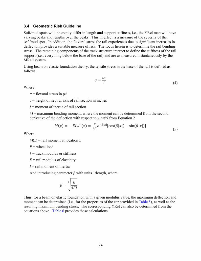
3.4 Geometric Risk Guideline Soft/mud spots will inherently differ in length and support stiffness, i.e., the YRel map will have varying peaks and lengths over the peaks. This in effect is a measure of the severity of the soft/mud spot. In addition, the flexural stress the rail experiences due to significant increases in deflection provides a suitable measure of risk. The focus herein is to determine the rail bending stress. The remaining components of the track structure interact to define the stiffness of the rail support (i.e., everything below the base of the rail) and are as measured instantaneously by the MRail system. Using beam on elastic foundation theory, the tensile stress in the base of the rail is defined as follows:

(4) Where

σ = flexural stress in psi c = height of neutral axis of rail section in inches I = moment of inertia of rail section M = maximum bending moment, where the moment can be determined from the second derivative of the deflection with respect to x, w(x) from Equation 2

(5) Where

M(x) = rail moment at location x P = wheel load k = track modulus or stiffness E = rail modulus of elasticity I = rail moment of inertia And introducing parameter β with units 1/length, where

Thus, for a beam on elastic foundation with a given modulus value, the maximum deflection and moment can be determined (i.e., for the properties of the car provided in Table 5), as well as the resulting maximum bending stress. The corresponding YRel can also be determined from the equations above. Table 6 provides these calculations.

25

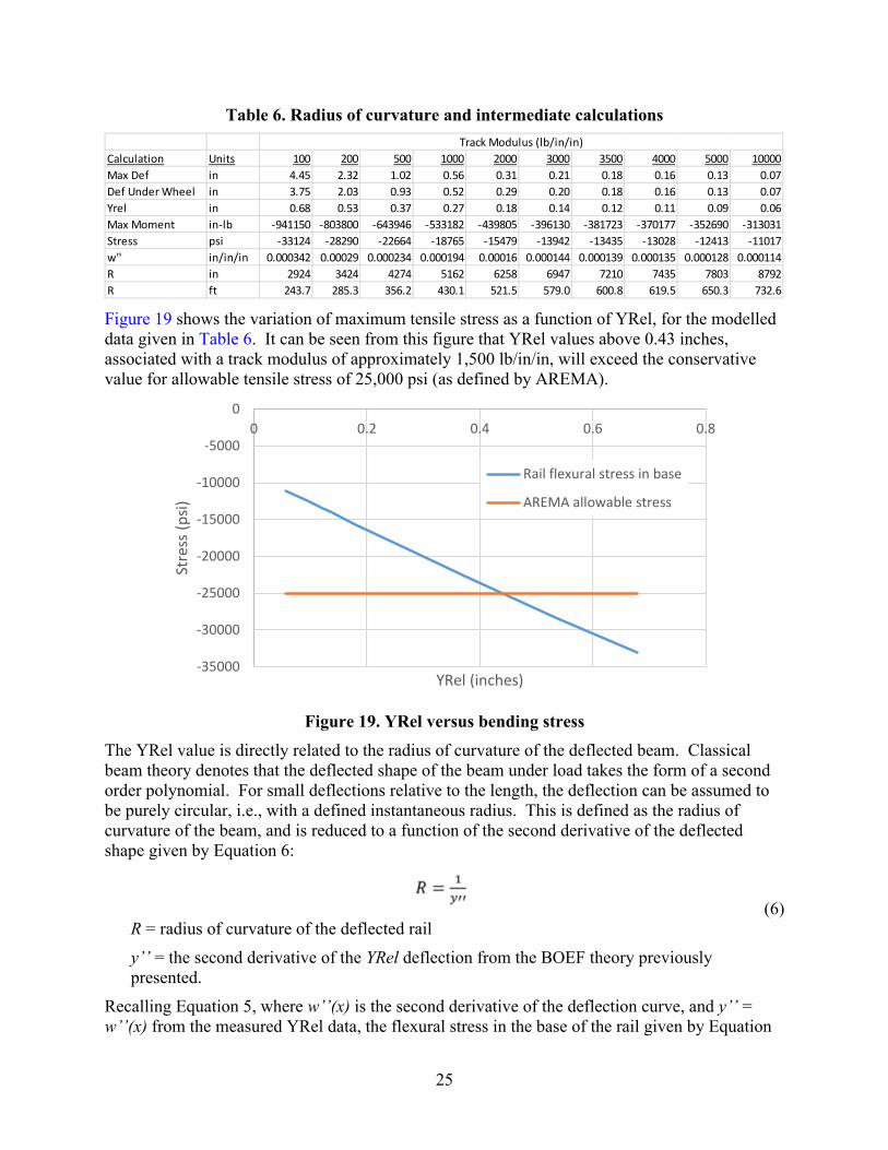
Table 6. Radius of curvature and intermediate calculations

Figure 19 shows the variation of maximum tensile stress as a function of YRel, for the modelled data given in Table 6. It can be seen from this figure that YRel values above 0.43 inches, associated with a track modulus of approximately 1,500 lb/in/in, will exceed the conservative value for allowable tensile stress of 25,000 psi (as defined by AREMA).

Figure 19. YRel versus bending stress

The YRel value is directly related to the radius of curvature of the deflected beam. Classical beam theory denotes that the deflected shape of the beam under load takes the form of a second order polynomial. For small deflections relative to the length, the deflection can be assumed to be purely circular, i.e., with a defined instantaneous radius. This is defined as the radius of curvature of the beam, and is reduced to a function of the second derivative of the deflected shape given by Equation 6:

(6) R = radius of curvature of the deflected rail y’’ = the second derivative of the YRel deflection from the BOEF theory previously presented.

Recalling Equation 5, where w’’(x) is the second derivative of the deflection curve, and y’’ = w’’(x) from the measured YRel data, the flexural stress in the base of the rail given by Equation

Calculation Units 100 200 500 1000 2000 3000 3500 4000 5000 10000Max Def in 4.45 2.32 1.02 0.56 0.31 0.21 0.18 0.16 0.13 0.07Def Under Wheel in 3.75 2.03 0.93 0.52 0.29 0.20 0.18 0.16 0.13 0.07Yrel in 0.68 0.53 0.37 0.27 0.18 0.14 0.12 0.11 0.09 0.06Max Moment in-lb -941150 -803800 -643946 -533182 -439805 -396130 -381723 -370177 -352690 -313031Stress psi -33124 -28290 -22664 -18765 -15479 -13942 -13435 -13028 -12413 -11017w'' in/in/in 0.000342 0.00029 0.000234 0.000194 0.00016 0.000144 0.000139 0.000135 0.000128 0.000114R in 2924 3424 4274 5162 6258 6947 7210 7435 7803 8792R ft 243.7 285.3 356.2 430.1 521.5 579.0 600.8 619.5 650.3 732.6

Track Modulus (lb/in/in)

-35000

-30000

-25000

-20000

-15000

-10000

-5000

00 0.2 0.4 0.6 0.8

Stre

ss (p

si)

YRel (inches)

Rail flexural stress in base

AREMA allowable stress

26

5 can be determined from the YRel measured data, along with a value for R, thus relating radius of curvature to flexural stress. Figure 20 shows the relationship between radius of curvature of the deflected shape and the resulting maximum tensile stress in the base of the rail. It can be seen from this figure that any radius less than 325 ft will result in a tensile stress above 25,000 lb./in/in (i.e., the AREMA allowable stress limit).

Figure 20. Radius of curvature of the deflected rail versus stress

However, the deflection of the rail along the track is not measured at every point using the measurement system, thus, the radius of curvature of the defected shape (R) cannot be directly determined. Only one specific location of YRel is measured that is indicative of the track stiffness at that location and is directly related to the flexural stress in the rail. As shown in Figure 17, a map of the peak YRel values is obtained from the system. For each soft/mud spot, the radius of curvature of the YRel map (r) can be obtained. This can be achieved by the following equation:

(7) Where

r = Radius of curvature of the YRel path L = Length of YRel map at the uplift zone y0 = Mean value of YRel in uplift zone ymax = Max value of YRel in mud spot

27

For the example mud spot shown in Figure 17, Figure 21 results with the pertinent parameters for calculating the radius of curvature (r) identified, as follows:

L = 19 feet ymax = 0.7” y0 = (-0.13” – 0.05”)/2 = -0.09”

Using Equation 7, and resolving units, results in a radius of curvature of the mud spot of r = 685 feet.

Figure 21. Risk parameters from measured data

Calculating the radius of curvature of the YRel path using Equation 7 provides a relative risk condition of the mud spot. The radius of curvature of the mud spot YRel map is compared to variable thresholds. To understand the relationship between the length of a mud spot (L) and the delta deflection difference (ymax-y0), Figure 22 illustrates radius of curvature for three arbitrary values; 2,000, 500, and 325 ft (i.e., the radius of curvature below which the AREMA allowable stress limit is exceeded) as a function of expected mud spot length and deflection change from the peak uplift. Thus, any mud spot with a length and delta deflection that falls below the R = 325 ft line would develop flexural stresses that exceed the AREMA allowable stress limit. The previous soft/mud spot example for a radius of curvature of the deflected beam, r = 685 ft is also shown (as the blue square), where delta deflection equals ymax - y0 = 0.9 inches and the length, L = 19 feet.

28

Figure 22. Radius of curvature based on mud spot length and central deflection change

from the peak uplift vs. specific radius of curvature values For large YRel values (peak down (ymax) – peak uplift (y0)) over a short length (L), a small radius of curvature for the mud spot (r) exists and is indicative of increased flexural stress. Conversely, large YRel values (peak down (ymax) – peak uplift (y0)) over a longer length result in reduced flexural stresses. The radius of curvature of the mud spot (r) provides a mechanism for classifying the instantaneous severity of the mud spot at the time of measurement, and thus radius of curvature (r) becomes the risk variable. Note, the lower the value of (r), the higher the risk.

3.5 Time Component for the Risk Guideline In addition to the geometric component of the risk guideline, it is important to understand the rate of degradation of the mud spot, i.e., the change in risk parameter with increased time or tonnage. Researchers analyzed a section of MRS track with known mud posts. MRS data was preferred because it offered repeated runs of the same location where CSX data did not. Specifically, the study focused on marker kilometer post (KM) 257.7 The railroad identified known mud spots at approximately KM 257.1 and 257.4. Figure 23 shows the YRel plots for this stretch of track for three inspection dates from August 2017 to June 2018. The YRel plots in Figure 23 show a significant variation along the track with several “spikes” in the down and uplift directions. In addition, there appears to be an average stiffness change (from softer to stiffer track) at KM 257.7 as well as some variation of the signature from one inspection to another. It is difficult to pinpoint discrete soft/mud spots from these plots, based on the signature from Figure 17, and the locations must be “zoomed” in.

7 Note, that while all measurements and analyses are in English units, the track at MRS is identified by kilometer post. Thus, longitudinal references to track location will use KM.

05

1015202530354045

0 0.2 0.4 0.6 0.8 1 1.2

Leng

th, L

(ft)

Delta Deflection, ymax-y0 (in)

Severity of Mud Spot

R = 2000 ft R = 500 ft R=325 ft R = 685 ft

29

Figure 23. KM 257 for multiple inspection runs

Figure 24 shows the same data as Figure 23, zooming in around KM 257.35. It can be seen from this figure that there are similarities in the signature, however, the correlation is not extremely pronounced. A longitudinal shift can also be seen in the data, which is very common for any autonomous inspection system.

30

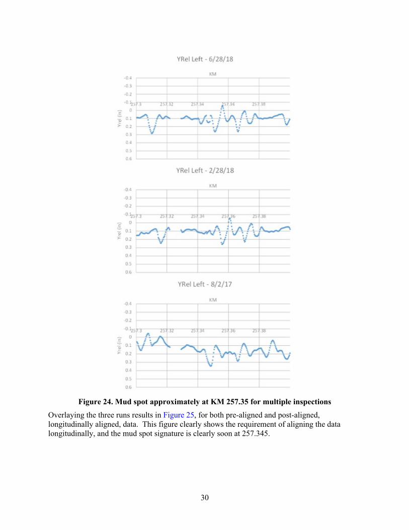
Figure 24. Mud spot approximately at KM 257.35 for multiple inspections

Overlaying the three runs results in Figure 25, for both pre-aligned and post-aligned, longitudinally aligned, data. This figure clearly shows the requirement of aligning the data longitudinally, and the mud spot signature is clearly soon at 257.345.

31

Figure 25. Overlaid and aligned YRel left data in vicinity of mud spot (KM 257.35)

Considering the data in Figure 25, the risk process can be applied, as defined in Equation 7, and risk parameters (r) determined for each date. Table 7 presents the results of this application, where Risk is r,8 the radius of curvature of the deflected rail, and is in feet. The smaller the value of Risk (r), the higher the flexural stress and possibly more urgent its maintenance priority.

8 Note, Risk (r), and radius of curvature are identical.

32

Table 7. Risk assessment of mud spot

KM 257.345

Date

Length (L) feet

Max Deflection

(ymax) inches

Mean Uplift (y0)

inches

Delta Deflection (ymax- y0) inches

Risk (r) feet

August 2, 2017 21 0.326 0.049 0.277 2388 February 28, 2018 23 0.257 -0.003 0.260 3057

June 28, 2018 21 0.259 0.012 0.247 2679

Table 7 shows that there is no direct correlation with time/traffic and the change in Risk (i.e., radius of curvature of the deflected shape). While the length remains relatively consistent, the peak values decrease over time and the risk value fluctuates. This is attributed to moisture content at the time of inspection and can vary by season or recent rainfall. This effect is shown graphically in Figure 26 for two mud spot areas.

Figure 26. Risk and peak deflection values over time for two mud spot locations

Figure 26 shows the risk (i.e., circles with left vertical axis scale) for two mud spots based on three inspections, as well as the peak deflection (i.e., triangles with right vertical axis scale) for the same mud spots and inspection dates. Recall that the risk is the radius of curvature of the deflected shape and is a function of the length and depth of deflection. The smaller the radius of curvature, the higher the risk (i.e., note gradient scale).

0.000

0.050

0.100

0.150

0.200

0.250

0.300

0.350

0.400

0.450

0.500

0

500

1000

1500

2000

2500

3000

3500

4000

4500

5000

06/17 08/17 09/17 11/17 12/17 02/18 04/18 05/18 07/18

Peak

(in)

Risk

, r (f

t)

Date of Inspection

Mud Spot Risk

KM 257.36 Risk KM 257.03 Risk

KM 257.36 Peak KM 257.03 Peak

33

4. Application of Risk Guideline

The risk guideline developed in the previous section was implemented on over nearly a thousand track miles of data.

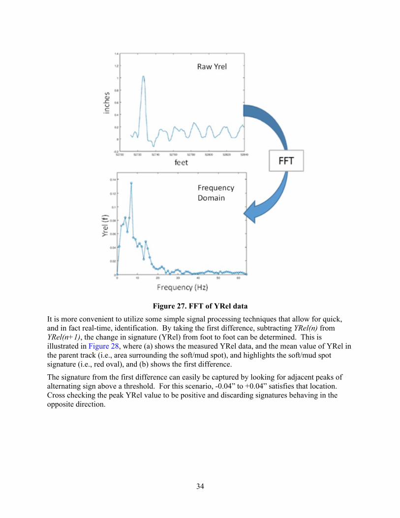
4.1 Soft/Mud Spot Identification To facilitate production analysis of mud spot data, researchers developed an algorithm for automatically identifying potential mud spots using signal processing techniques of the YRel signature. The signature shown in Figure 17 is fairly consistent, and depending on mud spot severity, will show changes in length and peak values. Machine learning techniques and other advanced data science techniques can be applied for identifying this signature. The first method for determining a “soft” location was to use Fast Fourier Transforms (FFTs). Using the signature shown in Figure 17, peak YRel with two uplift values, provides a unique signature that can be evaluated. To identify this signal, moving windows of YRel data were transformed into the frequency domain using FFT. Windows were required to isolate a specific signal response associated with one mud spot candidate and not the frequency spectrum of the entire dataset. Initial signal analysis was conducted using 40 ft windows (i.e., accounts for uplift zones of 18 ft mud spot). This initial window size was selected as it corresponded to twice the approximate average length of a small population of mud spot signatures identified via manual inspection of the data. Figure 27 shows an example of a 40 ft YRel data window being converted into the frequency domain using FFT. In the frequency domain, the signal was analyzed to identify the presence of a significant low frequency response. After complete processing, this window was flagged as a potential mud spot candidate. As can be seen, the YRel data shows the expected response (i.e., large peak flanked by minor deflection signals) and the frequency domain contains a significant low frequency response. This approach allows for automatically finding a location with the associated YRel signature that can be correlated to mud spots. This signature can now be prioritized for risk, as the length and maximum YRel will vary for each mud spot.

34

Figure 27. FFT of YRel data

It is more convenient to utilize some simple signal processing techniques that allow for quick, and in fact real-time, identification. By taking the first difference, subtracting YRel(n) from YRel(n+1), the change in signature (YRel) from foot to foot can be determined. This is illustrated in Figure 28, where (a) shows the measured YRel data, and the mean value of YRel in the parent track (i.e., area surrounding the soft/mud spot), and highlights the soft/mud spot signature (i.e., red oval), and (b) shows the first difference. The signature from the first difference can easily be captured by looking for adjacent peaks of alternating sign above a threshold. For this scenario, -0.04” to +0.04” satisfies that location. Cross checking the peak YRel value to be positive and discarding signatures behaving in the opposite direction.

35

Figure 28. Sample mud spot YRel (top/a) and first difference of YRel (bottom/b)

This algorithm can be applied in real time as well. Figure 29 show 0.6 miles of data (1 KM) and identified potential mud spots9 (orange dots).

Figure 29. 0.6 miles (1.0 km) of potential mud spots for a plot of left rail YRel data

9 These locations represent short localized soft spots in track and require validation to confirm if they are actual mud spots.

-0.4-0.3-0.2-0.1

00.10.20.30.40.50.6

129 129.1 129.2 129.3 129.4 129.5 129.6 129.7 129.8 129.9 130

Yrel

L (i

n)

Kilometer Post

36

Note that the YRel signature associated with a mud spot may also be associated with other soft support conditions in track. These may come from consecutive ties that are plate cut or excessively decayed, hanging ties, or other localized soft support conditions. Thus, the identification of localized soft support conditions in track is important, whether it be from a mud spot or other cause. To limit the analysis to just mud spots, visual inspection and validation of the locations must be performed at this time. While this can be time consuming and cumbersome, machine vision can be used to augment the MRail inspection system to automatically identify the presence of mud. However, all soft spots in track that are identified by the MRail data processing described should be investigated as to the root cause of localized deflection, i.e., mud spot, failed ties/fasteners, broken joint, etc. In addition, the algorithm may not identify newly formed mud spots until they reach peak deflection values that exceed the limits of detection.

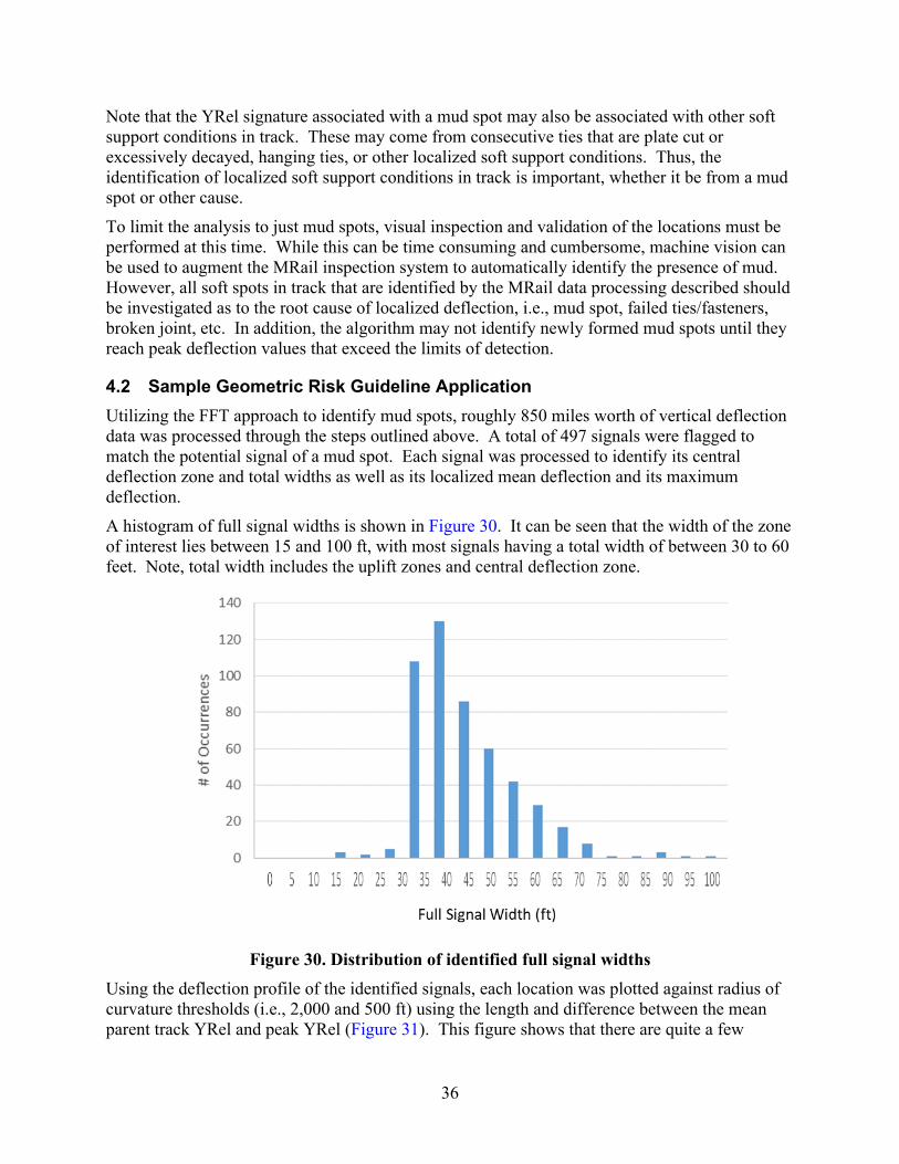
4.2 Sample Geometric Risk Guideline Application Utilizing the FFT approach to identify mud spots, roughly 850 miles worth of vertical deflection data was processed through the steps outlined above. A total of 497 signals were flagged to match the potential signal of a mud spot. Each signal was processed to identify its central deflection zone and total widths as well as its localized mean deflection and its maximum deflection. A histogram of full signal widths is shown in Figure 30. It can be seen that the width of the zone of interest lies between 15 and 100 ft, with most signals having a total width of between 30 to 60 feet. Note, total width includes the uplift zones and central deflection zone.

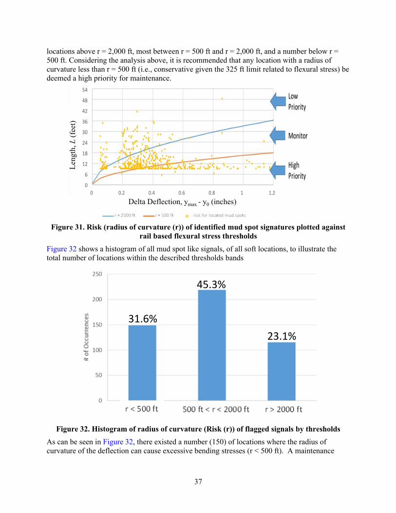
Figure 30. Distribution of identified full signal widths Using the deflection profile of the identified signals, each location was plotted against radius of curvature thresholds (i.e., 2,000 and 500 ft) using the length and difference between the mean parent track YRel and peak YRel (Figure 31). This figure shows that there are quite a few

37

locations above r = 2,000 ft, most between r = 500 ft and r = 2,000 ft, and a number below r = 500 ft. Considering the analysis above, it is recommended that any location with a radius of curvature less than r = 500 ft (i.e., conservative given the 325 ft limit related to flexural stress) be deemed a high priority for maintenance.

Figure 31. Risk (radius of curvature (r)) of identified mud spot signatures plotted against

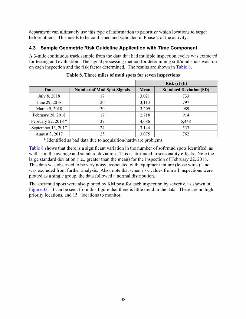
rail based flexural stress thresholds Figure 32 shows a histogram of all mud spot like signals, of all soft locations, to illustrate the total number of locations within the described thresholds bands

Figure 32. Histogram of radius of curvature (Risk (r)) of flagged signals by thresholds

As can be seen in Figure 32, there existed a number (150) of locations where the radius of curvature of the deflection can cause excessive bending stresses (r < 500 ft). A maintenance

Leng

th, L

(fee

t)

Delta Deflection, ymax - y0 (inches)0 0.2 0.4 0.6 0.8 1 1.2

0

6

12

18

24

30

36

42

48

54

31.6%

45.3%

23.1%

38

department can ultimately use this type of information to prioritize which locations to target before others. This needs to be confirmed and validated in Phase 2 of the activity.

4.3 Sample Geometric Risk Guideline Application with Time Component A 3-mile continuous track sample from the data that had multiple inspection cycles was extracted for testing and evaluation. The signal processing method for determining soft/mud spots was run on each inspection and the risk factor determined. The results are shown in Table 8.

Table 8. Three miles of mud spots for seven inspections Risk (r) (ft)

Date Number of Mud Spot Signals Mean Standard Deviation (SD) July 8, 2018 17 3,021 733

June 29, 2018 20 3,113 797 March 9, 2018 30 3,209 989

February 28, 2018 17 2,718 914 February 22, 2018 * 37 4,686 5,448 September 13, 2017 24 3,144 533

August 3, 2017 25 3,075 762 * Identified as bad data due to acquisition/hardware problems

Table 8 shows that there is a significant variation in the number of soft/mud spots identified, as well as in the average and standard deviation. This is attributed to seasonality effects. Note the large standard deviation (i.e., greater than the mean) for the inspection of February 22, 2018. This data was observed to be very noisy, associated with equipment failure (loose wires), and was excluded from further analysis. Also, note that when risk values from all inspections were plotted as a single group, the data followed a normal distribution. The soft/mud spots were also plotted by KM post for each inspection by severity, as shown in Figure 33. It can be seen from this figure that there is little trend in the data. There are no high priority locations, and 15+ locations to monitor.

39

Figure 33. Risk (r) values for 3 miles of soft/mud spots for seven inspections

Evaluating the data by inspection date, Figure 34 shows the mean risk (along with mean +/- one SD). Note that this figure excludes the date of February 22, 2018, as this data is suspect.

Figure 34. Plot of mean inspection session mud spot Risk (r) for the 3 miles inspection

location (six inspections) Figure 34 shows that on average, the risk remains fairly constant during this short time frame of data collection (i.e., less than 1 year), with some slight variation likely due to seasonality. In addition, the spread (i.e., standard deviation) varies over time, indicating a moisture content effect on the deflection and resulting risk factor. With more railway involvement, along with physical identification and validation of mud spots, the time dependent risk component previously discussed can be implemented. In addition,

0

1000

2000

3000

4000

5000

6000

44 45 46 47 48 49 50 51

Risk

, r (f

t)

KM

7/8/2018 6/29/2018 3/9/2018 2/28/2018 2/22/2018

9/13/2017 8/3/2017 High Priority Limit Monitor Limit

0

500

1000

1500

2000

2500

3000

3500

4000

4500

8/3/2017 9/22/2017 11/11/2017 12/31/2017 2/19/2018 4/10/2018 5/30/2018 7/19/2018 9/7/2018

Risk

, r (f

t)

Date of Inspection

Mean Mean - SD Mean + SD

40

maintenance activities can be evaluated as to their effect on mud spot remediation and reduction in risk.

41

5. Future Activities

The next phase of the project encompasses refinement and application of the risk algorithm on a defined section of track over a defined time period with close monitoring and cooperation by the partnering railway. Given the reliability issues with the hardware, Harsco has undertaken actions to make the hardware more robust. This was performed as a separate activity to ensure the reliability of the hardware during extensive use and was achieved by redesigning the sensor heads and employing hardening technology and environmental protection. To get a better understanding of the time and seasonal effects of the change in risk for a mud spot, more closely spaced inspections will need to be performed. It is expected that the risk will fluctuate up and down with an overall trend of increasing risk (decreasing r). The localized up and down trends will be attributed to moisture conditions at the time of inspection, and the overall trend will be attributed to the degradation of the mud spot. The following tasks/action plan are recommended for the second phase:

• Verify system reliability on MRail car and/or DOTX218

• Partner with Genesee & Wyoming Railroad to take regular measurements on stretch of track with known mud spot issues using the autonomous MRail hopper car

• Apply risk algorithm to provide alerts of high-risk mud spots

• Refine thresholds during course of measurement campaign based on field personnel input and onsite inspection o It is expected that the partnering railway will evaluate exceptions flagged by MRail

using experienced track engineering personnel along with experts from Harsco

• Document final recommendations

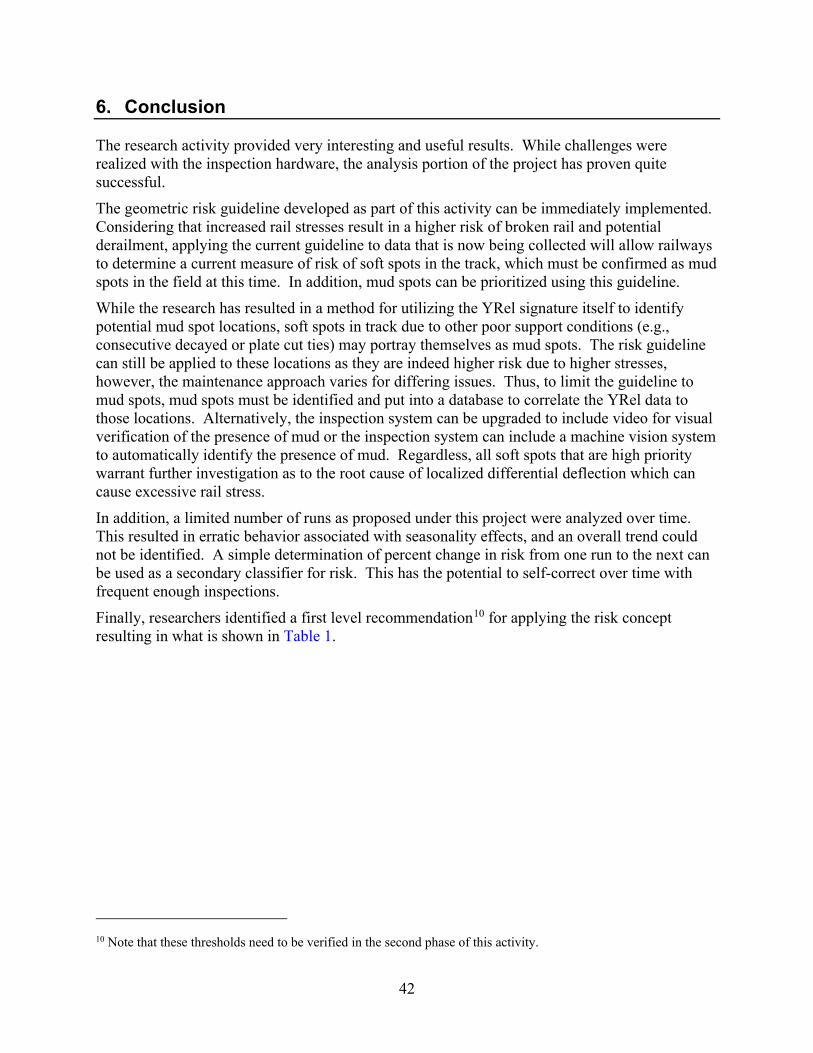
42

6. Conclusion

The research activity provided very interesting and useful results. While challenges were realized with the inspection hardware, the analysis portion of the project has proven quite successful. The geometric risk guideline developed as part of this activity can be immediately implemented. Considering that increased rail stresses result in a higher risk of broken rail and potential derailment, applying the current guideline to data that is now being collected will allow railways to determine a current measure of risk of soft spots in the track, which must be confirmed as mud spots in the field at this time. In addition, mud spots can be prioritized using this guideline. While the research has resulted in a method for utilizing the YRel signature itself to identify potential mud spot locations, soft spots in track due to other poor support conditions (e.g., consecutive decayed or plate cut ties) may portray themselves as mud spots. The risk guideline can still be applied to these locations as they are indeed higher risk due to higher stresses, however, the maintenance approach varies for differing issues. Thus, to limit the guideline to mud spots, mud spots must be identified and put into a database to correlate the YRel data to those locations. Alternatively, the inspection system can be upgraded to include video for visual verification of the presence of mud or the inspection system can include a machine vision system to automatically identify the presence of mud. Regardless, all soft spots that are high priority warrant further investigation as to the root cause of localized differential deflection which can cause excessive rail stress. In addition, a limited number of runs as proposed under this project were analyzed over time. This resulted in erratic behavior associated with seasonality effects, and an overall trend could not be identified. A simple determination of percent change in risk from one run to the next can be used as a secondary classifier for risk. This has the potential to self-correct over time with frequent enough inspections. Finally, researchers identified a first level recommendation10 for applying the risk concept resulting in what is shown in Table 1.

10 Note that these thresholds need to be verified in the second phase of this activity.

43

7. References

Li, D., Hyslip, J., Sussman, T., & Chrismer, S. (2016). Railway Geotechnics.Boca Raton, FL, USA: CRC Press

Kerr, A. D., (2003). Fundamentals of Railway Track Engineering. Omaha, NE, USA: Simmons-BoardmanBooks, Inc.

Farritor, S., “Measurement of Vertical Track Deflection for a Moving Rail Car,” Technical Report No. DOT/FRA/ORD-13/08, Washington, DC: U.S. Department of Transportation Federal Railroad Administration, February 2013.

Hogan, C., Dick, M., Lu, S., Farritor, S., Arnold, R., GeMeiner, W., & Clark, D., "Track Stiffness Measurement with Implementation to Rail/Vehicle Dynamic Simulation," Proceedings of the AREMA 2008 Annual Conference, Salt Lake City, UT, September 21–24, 2008.

Zarembski, A. M., Palese, Joseph, J. W., & Katz, L., “Implementation of a Dynamic Rail-Highway Grade Crossing Transition,” Transportation Research Board Annual Meeting, Washington, DC, January 1999.

44

Abbreviations and Acronyms

ACRONYMS EXPLANATION

AREMA American Railway Engineering and Maintenance-of-Way BOEF Beam on Elastic Foundation BAA Broad Agency Announcement FFT Fast Fourier Transform FRA Federal Railroad Administration GPS Global Positioning System KM Kilometer Post MP Milepost SD Standard Deviation