calculation of uptake of nutrients and water by a root system
TRANSCRIPT

NN33098*^°
I N S T I T U U T V O O R B O D E M V R U C H T B A A R H E I D
NOTA 210
CALCULATION OF UPTAKE OF NUTRIENTS AND WATER BY A ROOT SYSTEM
door
P. DE WILLIGEN
Bibliotheek AB-DLO Bornsesteeg 65 Postbus 14 6700 AA Wageningen
afbf9 1990
CENTRALE LANDBOUWCATALOGUS
0000 0707 4665

I N S T I T U U T V O O R B O D E M V R U C H T B A A R H E I D
NOTA 210
CALCULATION OF UPTAKE OF NUTRIENTS AND WATER BY A ROOT SYSTEM
door
P. DE WILLIGEN
Nota's van het Instituut voor Bodemvruchtbaarheid zijn in principe interne communicatiemiddelen en worden derhalve niet als officiele publikaties beschouwd. Zij zullen veelal resultaten van niet afgesloten onderzoek bevatten en/of als discussiestuk dienen. Eventuele conclusies mogen niet als definitief worden beschouwd. Deze nota's worden slechts in beperkte mate of in het geheel niet buiten het Instituut verspreid.
1990
Instituut voor Bodemvruchtbaarheid, Oosterweg 92, Postbus 30003, 9750 RA
Haren (Gr.)
CONTENTS
1. Introduction 2
2. Microscopic model of uptake of nutrients and water 3
2.1. Basic assumptions 3
2.2. Nutrients 3
2.3. Water 8
3. Description of uptake in a macroscopic model 10
3.1. Nutrients 10
3.2. Water 11
4. Programs 14
5. Examples 15
5.1. Water uptake 15
5.2. Nutrient uptake 18
6. Literature 21
Appendices
Appendix I. Calculation of the nutrient uptake by a single 23
root in a zero-sink situation
Appendix II. Numerical solution of radial flow of water to a 42
plant root
Appendix III. Calculation of uptake of a nutrient by a root system 67
Appendix IV. Calculation of water uptake by a root system 71

1. INTRODUCTION
Microscopic models on nutrient and water transport in the soil and on
uptake by the roots deal with gradients in the immediate vicinity of a
single root, i.e. with transport distances of a few millimeters or less.
Most of such models only consider transport in a horizontal direction,
transport being described in a fundamental way using Fick's and Darcy's
laws.
In macroscopic models (like crop growth models), on the other hand, the
scale is of the order of 10 cm or more and interest is focused on uptake
behaviour of a root system rather than that of a single root. Usually
transport in vertical direction is considered only, and fluxes of water are
calculated approximately, except where interest is in dynamics of water
flow per se.
Ideally, the description of uptake by a root system in a macroscopic
model should be based on the description of the uptake of a microscopic
model. More often than not, however, the macroscopic uptake models
(implicitly) lump effects of physical and physiological properties of soil
and roots into one or two parameters, of which it is often difficult to
comprehend how they quantatatively relate to the microscopic properties
they supposedly embrace.
The first goal of this report is to discuss how results of uptake models
on a microscopic scale can lead to a description of uptake on a macroscopic
scale consistent with the former. A second goal is to present a
documentation on the computer programs pertaining to the models discussed.

3
2. MICROSCOPIC MODEL OF UPTAKE OF NUTRIENTS AND WATER
2.1. Basic assumptions
For the microscopic model we start by considering a vertical cylindrical
root. The root is situated within a cylinder of soil. Over the outer
boundary of this cylinder no transport will take place. Such a root can be
thought of as belonging to a set of uniformly distributed roots all equally
active and of the same length.
The uptake rate is assumed to be constant and independent of the nutrient
concentration (water content or matric potential in case of water uptake)
as long as the latter exceeds a certain limiting value. This approach is
different from that of other workers in this field (Nye and Tinker, 1977;
Barber, 1984) who put most emphasis on the uptake-determining role of the
concentration.
Whenever the concentration (water content, matric potential) at the root
surface reaches its limiting value the uptake rate equals the rate of
arrival of the nutrient (water) at the root surface, i.e. the concentration
(water content) there will be maintained at the limiting value. In case of
the important nutrients N and K the limiting value can be safely set at
zero.
2.2 Nutrients
Analytical solutions
The system described in the foregoing paragraph can be formulated
mathematically by a partial differential equation, describing transport by
massflow and diffusion in a hollow cylinder, together with initial and
boundary conditions. The boundary condition at the inner cylinder (the
root) is either that of constant uptake or of zero-concentration.
De Willigen and van Noordwijk (1987) presented an analytical solution
when uptake is constant and the initial concentration is uniform. It reads
in dimensionless units (Table 1 explains the symbols):
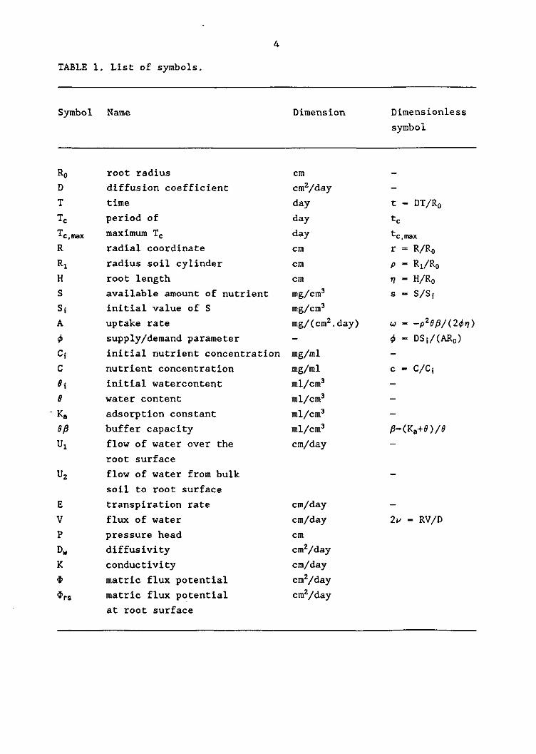
TABLE 1. List of symbols.
Symbol
Ro D
T
Tc
To, max
R
Ri H
S
Si A
<t> c,-c 0\ e Ka
op Ui
Name
root radius
diffusion coefficient
time
period of
maximum T c
radial coordinate
radius soil cylinder
root length
available amount of nutrient
initial value of S
uptake rate
supply/demand parameter
initial nutrient concentration
nutrient concentration
initial watercontent
water content
adsorption constant
buffer capacity
flow of water over the
Dimension
cm
cm2/day
day
day
day
cm
cm
cm
mg/cm3
mg/cm3
mg/(cm2.day)
-
mg/ml
mg/ml
ml/cm3
ml/cm3
ml/cm3
ml/cm3
cm/day
Dimensionless
symbol
-
t - DT/R0
tc
t-c.max
r = R/R0
P - Ri/Ro
1 = H/R0
s - S/Sj
w - -p26p/{24>r,)
<f> - DS,V(AR0)
-
c = C/Cf
-
-
-
P=(Ka+$)/0
-
u2
E
V
P
Dw
K
$
$ rs
root surface
flow of water from bulk
soil to root surface
transpiration rate
flux of water
pressure head
diffusivity
conductivity
matric flux potential
matric flux potential
at root surface
cm/day
cm/day
cm
cm 2 /day
cm/day
cm 2 /day
cm 2 /day
2i/ = RV/D

_ ( p 2 - l ) ( i / + l ) r (.Zu)
p2"*Z-l
U \2(u+\)r c *r !:rrp2Kp2(p_-r2n «. -JU71 2i-.2 2i / (p z T 7 r - l )
^ ( ^ - D r ^ d / f l ) ^ r 2 " ( ^ l ) (1-p2"*4) ] +
2u(p2v*2-l)2 ( 2^+4)(p 2"* z - l ) 2
<& ( W - 2 u ) r ^ £ J ^ l ( a n ) ^ i ( ^ n ) F i ) ( r Q n ) e ^ - ,
n.1 <*n n-l
< *
P n-l Q n
( l a )
( l b )
( l c )
( Id )
w i th :
F„(r,an) ^ l ( P Q n ) J
y ( r Q n ) - Yv(ran)JVfl(pan)
and an i s t he n - t h r oo t of:
W Q ) J , . i ( P Q ) " - W « ) > \ , - i ( p a ) - 0
Where J„(x), Y„(x) denote the Bessel function of the first kind, order v
and argument x and the modified Bessel function of the first kind order u
and argument x respectively. Eventually the series part (lc-d) will vanish
and a steady-rate situation, where concentration is a linear function of
time, will develop given by (la-lb). The uptake potential of the system can
be characterized by a characteristic time constant tu, called the period of
unconstrained uptake, denoting the period during which the concentration at
the root surface exceeds zero. If the concentration at the root surface
reaches its limiting zero-value in the steady-rate situation, at time t -
tu, the concentration profile can be given by:
f r 2 v 2
[2(p2"*2-l r2"(i/V*2)
) 2u(p Zi/-Z. 1) P2-2 1
lv{p2»*2-l)\ (2)
If after t - tu the concentration at the root surface is constant (zero),
i.e. the root behaves as a zero-sink, the concentration distribution for t
> tu is given by (De Willigen and Van Noordwijk in prep.):

«n<t-tu) (3)
where
Cv(ra) - Y^r^J^pa) - Jv(ra)Yvtl(pa)
and an now is the n-th root of Cu(a) - 0.
From (3) the uptake rate can be derived as the gradient of the
concentration c at the root surface (where r-1):
facl -4(t/+l)h> A JJi(pa) *2<t-i
(4)
From (4) the time-integrated uptake after the period of unconstrained
uptake is found as:
2 , v -«£(t-tu> fW dt- - M ^ l ) ^ V* •Jy.liP") {1 - W P Q ) d _ e W }
(5)
It now appears (De Willigen and Van Noordwijk 1987) that (4) can be
approximated very well by a much simpler equation viz. a steady-rate
equation like (2), but with time-dependent uptake rate wt, which is given
by:
(6)
A consequence of the assumption of the concentration being given by (2)
with o>t instead of u> is that the former is proportional to the average
concentration:
_ _ (P2-Dc
(7)
where the function G(p,v) is given by:

^ ' ; 2<«/*l)[T^ 2T 2i/(P2"2-l)
1-P2"»A) («/+!) ) >(/+4)(/>2"*2-l)J (2
and c denotes the average concentration in the soil solution.
The above solutions (i.e. (3), (4), (5) and the approximation (6)) pertain
to the situation where a steady-rate concentration profile (2) has
developed before the concentration at the root surface reaches zero. When
the concentration at the root surface drops to zero before the steady-rate
situation has been reached -thus before the terms (lc) and (Id) can be
neglected - it is assumed that the root behaves as a zero-sink from the
beginning. The exact solution for the concentration is now given by (De
Willigen and Van Noordwijk, unpublished):
a2t
c . ^ y 2vj2Aa n) - ̂ "^(ttJ-Wttn) r"C„(ran) ^ n-0 4(an) -Jl,(pan) P
v*l*n ' (8)
and that for uptake by :
fac] 2 y 2uJu{a)Jv^{pa) - ap"*1^ (pa) -St
(9)
whereas the time-integrated uptake now is given by:
i n-o oAjl(a) - J 2 , (pa)) °ij2A«) - JUP«)) ( 1 0 )
Here it also appeared that the the complicated expression for uptake (9)
can be very well approximated by an equation like (7).
Figure 1 shows the cumulative uptake in the zero-sink situation for the
exact solutions and the approximation. Details about the calculation
procedure are found in Appendix I. The approximation is shown to be quite
good, so it will be used in formulating uptake in the macroscopic model to
be discussed in section 3.1.

uptake (kg/ha) 400
200 250
time (days)
Figure 1. Cumulative uptake calculated with the exact solution (6) and the steady-rate approximation. Parameters: available amount 400 kg/ha, required uptake rate 2 kg/(ha.day), root length 20 cm, root radius 0.02 cm, transpiration 0.5 cm/day, diffusion coefficient 0.028 cm2/day, adsorption constant 20 ml/cm3. The lines give the exact solution; the points the steady-rate approximation. The figures at the curves denote the root length density in cm/cm3.
2.3. Water
Mathematical formulation The partial differential equation describing transport of water in the soil (Richards equation) is strongly nonlinear, which makes the finding of analytical solutions generally very difficult. We had to resort to numerical techniques to obtain a solution (see Appendix I I ) .
As shown earlier (De Willigen and Van Noordwijk, 1987) the numerical solution can be very well approximated by a steady-rate approximation similar to that given in (2), be it that it should be written in terms of the matric flux potential, which is defined as:
9sat
<*> f D„d8 - fadP
(11)

and that the limit for v — > 0 of (2) should be taken. The steady-rate solution in terms of the matric flux potential reads:
~2~n r2-l _ P
2lnr 2(P2-1) J*"-! (12)
where $rs is the matric flux potential at the root surface. The flow of water towards the root is then given as:
"''fr^A (13)
where G(p,0) is the function G(p,v) given earlier for v — > 0. Figure 2 shows the time course of water uptake in case of constant water
uptake until Prs, the pressure head at the root surface, equals 0.5 MPa, whereas thereafter Prs is kept constant at 0.5 MPa, calculated with the numerical model and with the steady-rate approximation (13). The approximation is shown to be quite satisfactory.
transpiration (cm) 30
10
time (days)
Figure 2. Cumulative transpiration calculated with the numerical model (lines) and with the steady-rate approximation (points). Transpiration was set constant at 0.5 cm/day, until the pressure head at the root surface reaches 5000 cm. Thereafter the pressure head is kept constant at 5000 cm. The figures at the curves denote the root length density in cm/cm3.

10
3. DESCRIPTION OF UPTAKE IN A MACROSCOPIC MODEL
3.1. Nutrients
The findings discussed in 2.2 can be used to describe uptake in a
macroscopic model, i.e. a model which deals with average values of
concentration and root density in horizontal layers. We first consider a
single layer with uniformly distributed roots. The potential uptake rate
from this layer is given by (7), i.e. the uptake rate in the zero-sink
situation. As long as this potential uptake rate exceeds the required
uptake rate the actual uptake rate equals the required uptake rate. When
the potential uptake rate is lower than the required uptake rate, actual
uptake rate equals potential uptake rate. The actual uptake rate is thus
the minimum of the required and the potential uptake rate. The total uptake
then simply is the sum of the uptake of the individual roots.
When different horizontal layers in the root zone are distinguished,
each with its own root density and nutrient concentration the situation is
more complicated. It is conceivable, as indeed is often found, that roots
in favourable position can compensate for roots in less favourable position
(De Jager, 1985). It is assumed therefore that the uptake rate of roots in
a certain layer depends on the uptake potential of roots in other layers.
Uptake now is calculated in an iterative way. First (step 1) the
nutrient demand is divided by the total root length to obtain the required
uptake per unit root length. Multiplying this by the root length in a given
layer yields the required uptake from that layer. If the potential uptake
rate exceeds the required uptake rate, uptake from this layer equals the
required uptake. If the potential uptake rate is less than the required
uptake rate, uptake from this layer equals the potential uptake rate. For
convenience, those layers where actual uptake equals potential uptake will
be indicated as layers of category 1.
The total uptake by the root system is the sum of the uptake rates of
the individual layers. If the uptake in each layer can proceed at the
required rate, total uptake equals nitrogen demand and no iteration is
required. If total uptake is less than nitrogen demand, it is checked
whether uptake from those layers where the concentration was sufficiently
high to meet the original demand (for that particular layer) can be raised
to increase total uptake, possibly enough to meet the total demand.
This is achieved as follows. In step 2, first the difference between
demand and total uptake, as calculated in step 1, is divided by the total
root length of those layers (category 2) that were able to satisfy the
required uptake rate of step 1. This yields an additional uptake rate. The
11
required uptake rate for layers of category 2, in step 2, now equals the
required uptake rate of step 1, augmented with the additional uptake rate.
It now is examined if the layer can satisfy the required uptake, i.e. if
its potential uptake rate still exceeds the new value of the required
uptake rate. If not, uptake rate from this layer equals potential uptake
rate. If all layers of category 2 can satisfy the required uptake of step
2, total uptake equals demand and the iteration ends. If none of the layers
of category 2 can satisfy the required uptake of step 2, i.e. if in all
layers of category 1 and 2 zero-sink uptake occurs, the iteration also
ends. If only a part of the layers of category 2 can satisfy the required
uptake of step 2, iteration proceeds to step 3, etc. Appendix III describes
the computerprogram of this procedure in detail.
This calculation procedure implies that roots growing under favourable
conditions will compensate as much as possible for roots growing under less
favourable conditions. It is thus assumed that information about the
necessary behavior, as far as uptake is concerned, is instantaneously
available throughout the complete root system.
The procedure described above can also be applied when roots within a
horizontal layer are not distributed uniformly. The layer then is divided
over a number of compartments within which root distribution can be assumed
uniform.
3.2 Water
As in 3.1 we start with considering a single layer of soil containing
vertical and uniformly distributed roots. The flow of water over the root
surface is supposed to be linearly related to the difference between the
plant water potential and the pressure head of the soil water at the root
surface (De Willigen and Van Noordwijk, 1987):
FH - kt (Prs-Pp) + k2 (14)
where FM is the flux of water in cm3/(cm root.day), Prs is the pressure head
in the soil at the root surface in cm, Pp is the plant water potential in
cm, and kx in cm/day and k2 in cm3/(cm root.day) are coefficients related to
the root conductivity.
If the thickness of the soil layer is Ax cm and the root length density
Lrv cm/cm3 , the uptake Ux in cm3 water per cm2 soil surface per day is
given by:
Ux - Lrv Ax FM - q(Prs - Pp) + v (15)

12
where
q - Lrv Ax k1( and v - Lrv Ax k2
We assume that no water can accumulate at the root surface, so that U:
equals the supply of water at the root surface. The flow from the bulk soil
in the layer with matric flux potential $ towards the rootsurface where the
matric flux potential is $rs is given by (cf (13)):
U2 - s(*rs - *) (16)
where
Ax (p2 - 1)
whereas there exists a functional relationship between $ and P (see
definition of * in (11)).
If the required uptake is given as Eact (the transpiration rate in
cm/day) the right hand side of (16) should equal Eact, and the resulting
equation can simply be solved for $rs. Using the inverse of (11) then Prs is
calculated. Finally because:
Ui - U2 - Eact
the plant water potential can be computed from (15) as:
Pp " Prs " (Eact " v)/q (17)
The situation is in fact more complicated because the actual transpiration
rate is a function of the plant water potential:
Eact " f(Pp) Epot (18)
where f(Pp) is a factor by which the potential transpiration Ep<jt has to be
reduced. As f(Pp) is a non-linear function of Pp, Eact and Prs have to be
found by iteration.
When the root system is distributed over n different layers, but roots
can be assumed to be distributed uniformly within a layer, for each layer
equations like (15) and (16) can be formulated. Equating these equations
one finds for the i-th layer:
13
qi(Prs,i " V + Vj - Sj($rsi - *,) (19)
It is assumed that the plant water potential Pp is identical everywhere in
the root system. In total then one obtains n equations of the form of (19),
and n+1 unknowns i.e. Prsl - Prsn (where again (11) can be used to
calculate * from P or vice-versa) and Pp. When the uptake rate Eact is known
an additional equation states that the sum of the flows over the
rootsurface in each layer from the root zone equals Eact:
n
(20)
When one takes into account the relation between plant water potential and
uptake rate equation (18) has to be used. Because of the non-linearity of
(11) and (18) the solution has to be found by iteration. Appendix IV gives
the details.

14
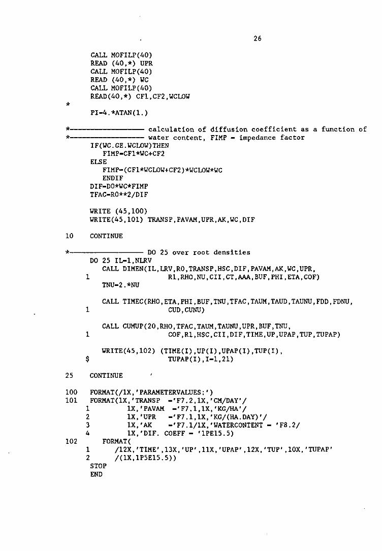
4. PROGRAMS
Calculations were performed with the computerprograms shown in appendices
I-IV. All programs are written in Fortran. The programs consist of a number
of subprograms (Fortran subroutines and functions), each dealing with a
specific part of the calculations. The programs are organized and
documented according to recommendations of Van Kraalingen and Rappoldt
(1989).
15
5. EXAMPLES
5.1 Water uptake
As an example results of Sharp and Davies (1985) will be used. They
performed an experiment on water uptake and root growth of maize plants.
Individual plants were grown in soil columns of 80 cm height. After a
preliminary growth period of two weeks the plants were subjected to two
treatments. Half of the plants were watered daily, where care was taken
that the soil water was replenished up to field capacity, the other half
did not get any water at all for the 18 day experimental period. Every
three days some columns were harvested and soil water content, root length
distribution, total dry matter and its distribution were measured, as well
as, prior to harvesting, the leaf water potential. Soil water depletion
rates were calculated from the changes in soil water content between
successive sampling days.
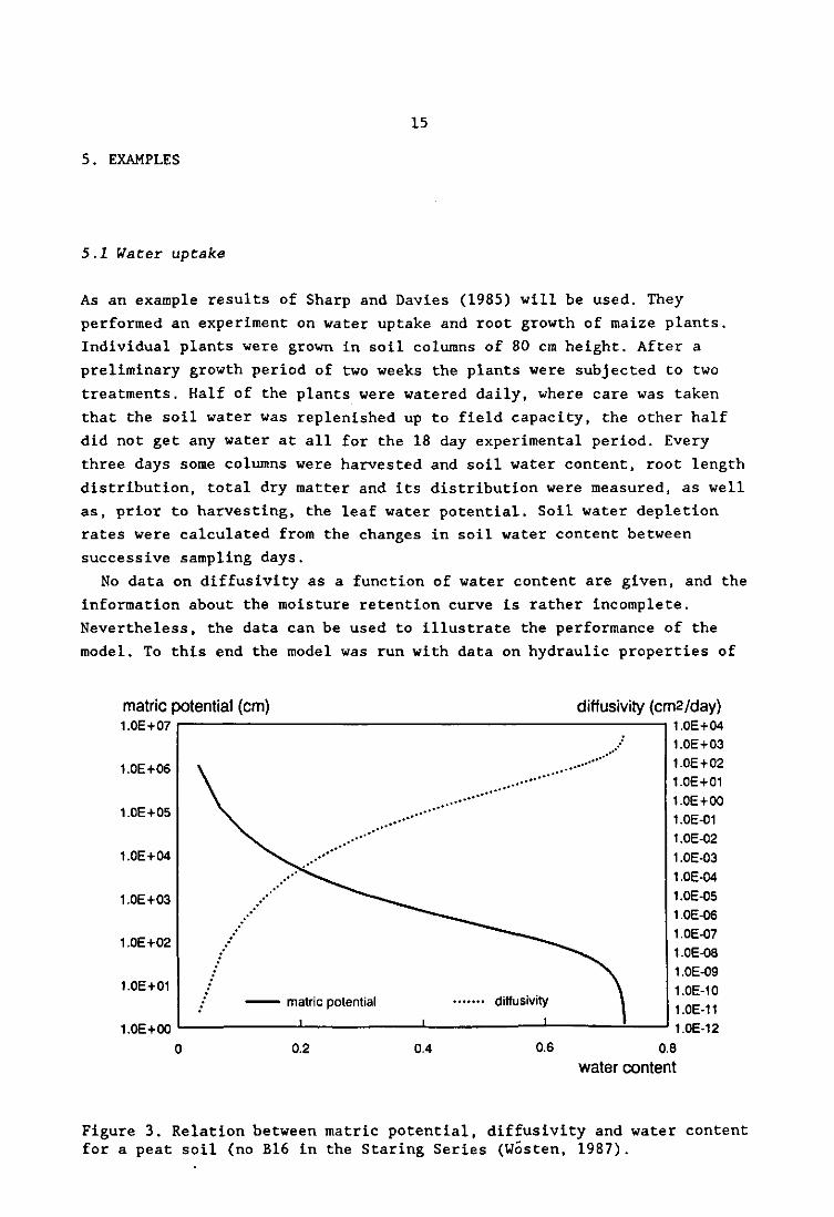
No data on diffusivity as a function of water content are given, and the
information about the moisture retention curve is rather incomplete.
Nevertheless, the data can be used to illustrate the performance of the
model. To this end the model was run with data on hydraulic properties of
matric potential (cm) diffusivity (cm2/day) l.Ut + U/
1.0E+06
1.0E+05
1.0E+04
1.0E+03
1.0E+02
1.0E+01
^v .»•**"
N ^ ' ' '
« ^ ^
/
."
— matric potential
_...••*"
,..•"*
i '
0.2 0.4
1.0E+04 1.0E+03 1.0E+02 1.0E+01 1.0E + 00 1.0E-01 1.0E-02 1 .OE-03 1.0E-04 1.0E-05 1 .OE-06 1 .OE-07 1 .OE-08 1 .OE-09 1.0E-10 1.0E-11 1.0E-12
0.6 0.8
water content
Figure 3. Relation between matric potential, diffusivity and water content for a peat soil (no B16 in the Staring Series (Wosten, 1987).

16
matric potential (cm) 1.0E + 05
1.0E+04
1.0E+03
1.0E+02
1.0E+01
1.0E+00
diffusivity (cm2/day) 1.0E+04
matric potential diffusivity
j L
0.1 0.2 0.3
1.0E+03
1.0E+02
1.0E+01
1.0E+00
1.0E-01
1.0E-02
1.0E-03
1.0E-04
1.0E-05
0.4 0.5
water content
Figure 4. Relation between matric potential, diffusivity and water content for a sandy loam (Lovl2c data from Boekhold, 1987).
two soils: one a sandy loam (Lovl2c; Boekhold, 1987) the other a peaty soil
(B16; Wosten, 1987). Figures 3 and 4 depict the relation between water
content, pressure head and diffusivity of these two soils.
Figures 5 and 6 give the results for day 15 for the two treatments. In
the treatment where the soil was kept at field capacity (figure 5)
distribution of uptake with depth was similar to the root density
distribution. In the calculations it was assumed that soil water was in
equilibrium with a groundwater table at a depth of 80 cm, the length of the
soil tube. According to the calculations at every depth in the transport
chain: bulk soil > root surface > root, the highest resistance was
experienced by the transport over the root wall. The overall resistance was
therefore lowest where root density was highest, which results in uptake
being more or less proportional to root density. Because of the dominance
of the root resistance the results for the two soils were practical
identical, differences in calculated uptake being less than 0.01%.
The results for the unwatered treatment are given in figure 6. The
pressure head at every depth was estimated from the reported water content.
Now the soil resistance is, except for the deepest layer, higher than the
root resistance, so distribution of uptake is quite different from root
density distribution. Moreover, the results for the two soils now clearly

17
depth (cm) 0
o
root density (cm/cm3)
70
calculated lovl 2c — — measured root density
0.1 0.2 0.3 0.4 0.5
uptake (cm/day)
Figure 5. Measured and calculated depth-distribution of water uptake and root-density of a maize-plant in a soil kept at field capacity. Data from Sharp and Davies (1985). For the calculations the hydraulic properties of Lovl2c (figure 4) have been used.
depth (cm) ° 0
0.5
root density (cm/cm3) 1.5 2
0.4 0.5
uptake (cm/day)
calculated Lov12c
root density
' " " • measured
calculated peat b16
Figure 6. As figure 5, but in a soil which has not been watered during 15 days. For the calculations the hydraulic properties of Lovl2c (figure 4) and B16 (figure 3) have been used.

18
differ, those for Lovl2c being more or less similar to the measured
results. The results of the peat B16 differ considerably from the
measurements. On this soil in the upper two layers negative water uptake
occurs according to the calculations, i.e. water flows out of the root to
the soil. This may be an artefact due to the assumption of uniform plant
water potential, but on the other hand such a phenomenon is often
established experimentally (e.g. Baker and Van Bavel, 1986).
5.2. Nutrient uptake
To illustrate the possibilities of the nutrient uptake model, the water
uptake pattern and water content distribution as found by Sharp and Davies
(1985) discussed in 5.1 were used.
Four situations were considered: the two treatments of water application
mentioned in section 5.1 with the corresponding root length distributions,
and two different distributions of mineral nitrogen in the soil. In one of
the chosen distributions every soil layer contains 1 kg/ha, except the
upper 10 cm where mineral nitrogen amounts to 20 kg/ha, in the other this
amount is found in the layer 40-50 cm. The required uptake rate of the
maize plants was estimated from the transpiration rate assuming a
transpiration coefficient of 350 kg/kg and an assumed nitrogen content of
2.5%. For the adequately watered plants the required uptake calculated in
this fashion amounted to 8.8 kg/(ha.day), for the unwatered plants to 6
kg/(ha.day).
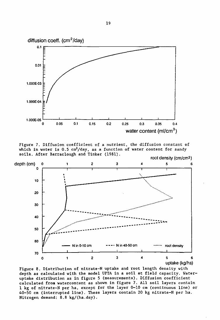
The effective diffusion coefficient of ions in soil is strongly
influenced by the water content. It can be calculated as:
D - D0f{t (21)
where D0 is the diffusion coefficient of the ion in free water, and f̂ an
impedance factor. The latter is a function of 9 as well. Figure 7 gives the
diffusion coeffient as a function of the water content using the relation
between impedance factor and water content as established by Barraclough
and Tinker (1981) for sandy and sandy loam soils. This relation has been
used in the model calculations.
Figures 8 and 9 show the results. For the adequately watered plants the
distribution of nitrogen has no effect, whereas in the dry situation
concentration of nitrogen in deeper moister layers is much more favourable,
the realized uptake rates being 1.5 and 4.5 kg/(ha.day) respectively.
19
diffusion coeff. (cm2/day)
0.01 E
1.000E-03 =
1.000E-04
1.000E-05
water content (ml/cm )
Figure 7. Diffusion coefficient of a nutrient, the diffusion constant of which in water is 0.5 cm2/day, a s a function of water content for sandy soils. After Barraclough and Tinker (1981).
root density (cm/cm3) depth (cm) 0 1 2 3 4 5 6
u
10
20
30
40
50
60
-
/ „ •
f-.^*
•
I I I
t 1 _ 1 ^ _ „ — - - " - ^ — 1 1
/ * ~ r. ** •* • • •
N in 0-10 cm N in 40-50 cm
1 1 1
1 T - •
'••.
* V
" - • • * *
1 '
0 1 2 3 4 5 6
uptake (kg/ha) Figure 8. Distribution of nitrate-N uptake and root length density with depth as calculated with the model UPTA in a soil at field capacity. Water-uptake distribution as in figure 5 (measurements). Diffusion coefficient calculated from watercontent as shown in figure 7. All soil layers contain 1 kg of nitrate-N per ha, except for the layer 0-10 cm (continuous line) or 40-50 cm (interrupted line). These layers contain 20 kg nitrate-N per ha. Nitrogen demand: 8.8 kg/(ha.day).

20
depth (cm) o o
10
20
30
40
50
60
70
0.5
root density (cm/cm3) 1.5 2
«.-•*-•
N in 0-10 cm N in 40-50 cm
I
root density
4 5
uptake (kg/ha)
Figure 9. As fig 8 but in a soil which has not been watered during 15 days. Water-uptake distribution as in figure 6 (measurements). Nitrogen demand: 6 kg/(ha.day).

21
6. LITERATURE
Baker J M and LC H M Van Bavel, 1986. Resistance of plant roots to water
loss. Agron J 78: 641-644.
Barber S A, 1984. Soil nutrient bioavailability: a mechanistic approach.
New York, John Wiley, 398 pp.
Barraclough P B and P B Tinker, 1981. The determination of ionic diffusion
coefficients in field soils. I. Diffusion coefficients in sieved soils in
relation to water content and bulk density. J Soil Sci 32: 225-236.
Boekhold A E 1987. Waterbeweging en stoffentransport in de onverzadigde
zone van de bodem: Invloed van bodemfysische eigeschappen op watergehalte
profielen en tijd-diepte curven, Inst. Bodemvruchtbaarheid, Nota 171, 35
pp.
De Jager A, 1985. Response of plants to a localized nutrient supply. PhD
Thesis, University of Utrecht, 137 pp.
De Willigen P and M Van Noordwijk, 1987. Roots, plant production and
nutrient use efficiency. PhD Thesis, Agricultural University Wageningen,
280 pp.
Forsythe G E, M A Malcolm and C B Moler, 1977. Computer methods for
mathematical computations. Prentice-Hall, Inc. Englewood Cliffs, 260 pp.
Lindelof T., 1981. Cern Computer Centre Program Library Manual, CERN
Geneva, Switzerland.
Nye P H and P B Tinker, 1977. Solute movement in the soil-root system.
Sudies in ecology, vol. 4. Oxford, Blackwell Scientific Publications, 342
PP.
Patankar S V, 1980. Numerical heat transfer and fluid flow. Hemisphere
Publishing Corporation, New York etc., 183 pp.
Sharp R E and W J Davies, 1985. Root growth and water uptake by maize
plants in drying soil. J Expt Bot 36: 1441-1456.

22
Ten Berge H F M , 1986. Heat and water transfer at the bare soil surface.
PhD Thesis, Agricultural University Wageningen, 214 pp.
Van Genuchten M Th, 1980. A closed-form equation for predicting the
hydraulic conductivity of unsaturated soils. Soil Sci. Soc. Am. J. 44: 892-
898.
Van Kraalingen D W G and C Rappoldt, 1989. Subprograms in simulation
models. Simulation Report CABO-TT nr 18, 54 pp.
Wosten J H M 1987. Beschrijving van de waterretentie- en
doorlatendheidskarakteristieken uit de Staringreeks met analytische
functies. STIBOKA Rapport 2019, 53 pp.

23
APPENDIX I. Calculation of the nutrient uptake by a single root in a zero-sink situation.
The relation between the subroutines is given in figure AI-1. The subroutine DIMEN calculates dimensionless parameters p, r/, <f>.
These are used in TIMEC, which calculates the period of unconstrained uptake both in dimensionless and absolutes units.
Relational diagram of subroutines in MDZER
f MDZER *) (
DIMEN )
{^CUMUP^) (̂ TERM ̂ (̂ ZEJY1 ^ ) -
-(^ TIMEC ̂ )
GRNU J BESFRY
)
-Tsumj -TBESFRJ ̂
-/SUM2J)
The core of the program is formed by the subroutine CUMUP which calculates the uptake and cumulative uptake after the period of unconstrained uptake, both exact and approximately. When the period of unconstrained uptake is less than zero, indicating that the concentration at the root surface drops to zero before a steady-rate situation has been developed, the calculations pertain to (9) and (10), otherwise to (4) and (5). CUMUP calls TERM, which calculates the terms of the summation series of (4), (5), (9), and (10), thereby using subroutine ZEJY1 which calculates the zero's an of the crossproduct given in the context of (3).
In the program the uptake rate (UP), the cumulative uptake (TUP), and their approximations (UPAP resp. TUPAP) are calculated in non-dimensionless form. In case of zero-sink uptake from the beginning the uptake rate in kg/(ha.day) is calculated as:
Wf-
and a similar expression is used to calculate TUP. The factor 100 converts the units from mg/cm2 to kg/ha.

24
If the period of unconstrained uptake is larger than zero, UP is calculated using:
UP/UPR - wt/u
where UPR is the uptake rate (in kg/ha) in the period of unconstrained uptake. The cumulative uptake TUP is the sum of the total uptake in the period of unconstrained uptake and the integral of UP in time.

REAL LRV(20),TIME(50),UP(50) REAL UPAP(50),TUP(50),TUPAP(50) INTEGER NC(20) REAL NU
Input data DATA TOL,DO/1.E-5,0.5/
OPEN (FILE-'MDZER.OUT'.UNIT-45) OPEN (FILE-'MDZER.INP'.UNIT-40) OPEN (FILE-'MASZER.LOG'.UNIT-46)
CALL MOFILP(40) READ (40,*) NLRV CALL MOFILP(40) READ (40,*) (LRV(I),I-1,NLRV) CALL MOFILP(40) READ (40,*) RO CALL MOFILP(40) READ(40,*) HSC CALL MOFILP(40) READ (40,*) AK CALL MOFILP(40) READ (40,*) TRANSP CALL MOFILP(40) READ (40,*) PAVAM
25
*___—_—_____ _____ * * Program MDZER.FOR * * Purpose: Calculation of diffusion and massflow of a nutrient * * to a root. Zero-sink solution. Replenishment of water at outer boundary * * FORMAL PARAMETERS: (I-input,0-output,C-control,IN-init,T-time) * * name type meaning units class * * * * R0 R4 radius root cm I * * DO R4 diffusion coefficient in free water cm2/day I * * DIF R4 diffusion coefficient in soil cm2/day 0 * * CF1 R4 coefficients for relation between * * CF2 R4 impedance and water content * * TFAC R4 ratio between real and dimensionless time day 0 * * * * SUBROUTINES called: * * DIMEN: calculates dimensionless variables * * TIMEC: calculates time constants * * CUMUP: calculates uptake rates * * * * File usage: * * MDZER.INP: contains input-data * * MDZER.OUT: detailed output on uptake, cumulative uptake, parameters * * * •k , •%
26
CALL MOFILP(40) READ (40,*) UPR CALL M0FILP(40) READ (40,*) WC CALL M0FILP(40) READ(40,*) CF1,CF2,WCL0W
*
PI«4.*ATAN(1.)
* calculation of diffusion coefficient as a function of * water content, FIMP - impedance factor
IF(WC.GE.WCLOW)THEN FIMP-CF1*WC+CF2
ELSE FIMP-(CF1*WCL0W+CF2)*WCL0W*WC ENDIF
DIF-D0*WC*FIMP TFAC-R0**2/DIF
WRITE (45,100) WRITE(45,101) TRANSP,PAVAM,UPR,AK,WC,DIF
10 CONTINUE
* DO 25 over root densities DO 25 IL-l.NLRV
CALL DIMEN(IL,LRV,RO,TRANSP,HSC,DIF,PAVAM,AK,WC,UPR, 1 R1,RH0,NU,CII,CT,AAA,BUF,PHI,ETA,C0F)
TNU-2.*NU
CALL TIMEC(RHO,ETA,PHI,BUF,TNU,TFAC,TAUM,TAUD,TAUNU,FDD,FDNU, 1 CUD.CUNU)
CALL CUMUP(20,RHO,TFAC,TAUM,TAUNU,UPR,BUF,TNU, 1 COF.Rl.HSC.CII.DIF,TIME.UP.UPAP,TUP,TUPAP)
WRITE(45,102) (TIME(I),UP(I),UPAP(I),TUP(I), $ TUPAP(I),1-1,21)
25 CONTINUE
100 FORMAT(/1X,'PARAMETERVALUES:') 101 FORMAT(IX,'TRANSP -'F7.2,IX,'CM/DAY'/
1 lX.'PAVAM -'F7.1,IX,'KG/HA'/ 2 IX,'UPR -'F7.1,1X,'KG/(HA.DAY)'/ 3 IX,'AK -'F7.1/lX,'WATERCONTENT - 'F8.2/ 4 lX.'DIF. COEFF - '1PE15.5)
102 FORMAT( 1 /12X,'TIME',13X,'UP',11X,'UPAP',12X,'TUP',10X,'TUPAP' 2 /(1X.1P5E15.5)) STOP END

27
maximum uptake period and related parameters
FORMAL PARAMETERS: (I-input,0-output,C»control,IN=init,T-time) name type meaning units class
RHO ETA PHI NU BUT TAUM
R4 R4 R4 R4 R4 R4
TAUD R4
TAUNU
FDD
FDNU
CUD
R4
R4
R4
R4
CUNU R4
Dimensionless radius soil cylinder Dimensionless root length Dimensionless supply parameter Dimensionless flux of water Buffer capacity Dimensionless maximum period of unconstrained uptake Dimensionless period of unconstrained uptake transport by diffusion only Dimensionless period of unconstrained uptake transport by diffusion and massflow Fractional depletion by unconstrained uptake transport by diffusion only Fractional depletion by unconstrained uptake transport by diffusion and massflow Fraction left at end of period of unconstrained uptake, transport by diffusion only Fraction left at end of period of unconstrained uptake, transport by diffusion and massflow
none Subroutines called Functions called :
GRNU: calculates G-function
File usage: time constants written to MDZER.OUT
I I I I I 0
* Subroutine TIMEC * Purpose: Calculation time constants, period of unconstrained uptake, * * * * * * * * * * * * * * * * * * * * * * * * * * * * * * *—
0 0
-* * * * * * * * * *
* * * * * * * * * * * * * * * * * * * * * *
-*
*-*-*-
SUBROUTINE TIMEC(RHO,ETA,PHI,BUF,TNU,TFAC,TAUM,TAUD,TAUNU,FDD, 1 FDNU,CUD,CUNU)
Calculation period of unconstrained uptake TAUNU, maximum TAUM
RH02-RHO**2 TAUM-(RH02-1.)/RH02*ETA*PHI TAUD-TAUM-BUF*GRNU(0.,RHO) TAUNU-TAUM-BUF*GRNU(TNU,RHO) FDNU-TAUNU/TAUM FDD-TAUD/TAUM CUNU-l.-FDNU CUD-1.-FDD
TM=TFAC*TAUM

28
TD-TFAOTAUD TN-TFAC*TAUNU WRITE(45,206) TM,TAUM,TD,TAUD,TN,TAUNU
206 F0RMAT(/15X,'TIME-CONSTANTS'/3IX,'DAYS',11X,'DIML' 1 /1X,'MAXIMUM:'12X.1P2E15.5/1X,'DIFFUSION :'9X,1P2E15.5 2 /1X/DIF. AND MASS FLOW :'1P2E15.5)
RETURN END

29
*
* PHI * ETA *
SUBROUTINE DIMENCIL.LRV.RO.TRANSP.HSCDIF.PAVAM.AK.UC.UPR, 1 Rl,RHO,NU,CII,CT,AAA,BUF,PHI,ETA,COF)
DIMENSION LRV(30) REAL LRV.NU
PI-4.*ATAN(1.) R1-1./SQRT(PI*LRV(IL)) RHO-R1/RO RH02-RHO**2 TNU--Rl**2*TRANSP/(2.*DIF*HSC*(RH02-1.))*(RH02-1.) NU-TNU/2. BUF-WC+AK CII-0.01*PAVAM/(HSC*BUF) CT-CII*BUF AAA-UPR/100. PHI-DIF*CT/(AAA*RO) ETA-HSC/RO COF-4.*(NU+l.)/(RHO**(TNU+2.)-l.)
VRITE(45,102) LRV(IL) WRITE(45,103) R1.RHO.RH02.PHI.ETA.TNU RETURN
* Subroutine DIMEN * * Purpose: calculation of dimensionless parameters * * FORMAL PARAMETERS: (I-input.O-output.C-control.IN-init.T-time) * * name type meaning units class *
* *
cm I * * LRV R4 Root length density cm/cm3 I * RO R4 Radius root c m j * TRANSP R4 transpiration rate cm/day I * * HSC R4 Root length c m I * * DIF R4 Diffusion coefficient soil cm2/day I * * PAVAM R4 Potential available amount of nutrient kg/ha I *
AK R4 Adsorption constant nutrient _ I * * WC R4 Water content _ I * * UPR R4 Uptake rate nutrient kg/(ha.day) I * * Rl R4 Radius soil cylinder c m 0 * * RHO R4 Dimensionless radius soil cylinder _ 0 * * NU R4 Dimensionless flux of water _ 0 * * CII R4 Initial concentration nutrient mg/ml 0 * * CT R4 Bulk density of nutrient mg/cm3 0 * * AAA R4 Uptake rate mg/(cm2.day) 0 * * BUF R4 Buffer capacity _ 0
R4 Dimensionless supply parameter _ 0 R4 Dimensionless root length _ 0
0 * * * * * *
* Subroutines/Functions called:none
File usage: dimensionless parameters written to MDZER.OUT *

30
102 FORMAT(//'************** LRV - '1PE15.5,2X,'**************'/ 1 IX,'COMBINED AND DIMENSIONLESS PARAMETERS')
103 F0RMAT(1X,'R1 -'1PE15.5,IX,'CM'/1X,'RHO -'1PE15.5, 1 1X,'RH02 -'1PE15.5/1X 2 'PHI -'1PE15.5/1X/ETA -'1PE15.5.1X/1X 3 'TNU -'1PE15.5)
END

31
* __ *
* Subroutine TERM * * Purpose: calculates N terms form the series part of zero-sink solution * * concerning uptake of nutrients. The terms TE1 and TE2 pertain * * to steady-rate initial condition, TE3 and TE4 to constant * * initial condition * * FORMAL PARAMETERS: (I-input,0-output,Ocontrol,IN-init,T-time) * * name type meaning units class * * * * RHO R4 dimensionless root density, i.e. the radius - I * * of the soil cylinder Rl over the root radius * * RO * * FL R4 Dimensionless flux of water - I * * TE1 R4 Term of solution for integrated uptake - 0 * * TE2 R4 Term of solution for uptake rate - 0 * * TE3 R4 Term of solution for integrated uptake - 0 * * TE4 R4 Term of solution for uptake rate - 0 * * N 14 Number of terms - I * * AL R4 Zero's from crossproduct of Bessel-functions: - 0 * * Y(FL,AL)J(FL+1,AL) - J(FL,AL)Y(FL+1,AL) - 0 * *
*
*-SUBROUTINE TERM(RH0,FL,TE1,TE2,TE3,TE4,N,AL) REAL TE1(N),TE2(N),TE3(N),TE4(N),AL(N),BJ(2) REAL JNA.JN1RA
DO 5 I-l.N * Calculation of AL(I)
CALL ZEJYl(AL(I),I,RHO,FL,20.,l.E-5,6) WRITE(46,*) 'I. AL »,I,AL(I)
*. * . Calculation of Bessel function J, with order FL * — and argument AL(I)
CALL BESFRJ(AL(I),FL,6,BJ)
JNA-BJ(l)
* Calculation of Bessel function J, with order FL+1 * and argument AL(I)*RHO
RA-RHO*AL(I) CALL BESFRJ(RA,FL,6,BJ) JN1RA-BJ(2)
TE1(I)-JN1RA**2/(AL(I)**4*(JNA**2-JN1RA**2)) TE2(I)-TE1(I)*AL(I)**2
* * Subroutines called: * * ZEJY1 : calculates zero's from crossproduct of Bessel-functions: * * Y(FL,AL)J(FL+1,AL) - J(FL,AL)Y(FL+1,AL) - 0 * * BESFRJ : Bessel function of first kind and fractional order *
* * Functions called: none ^ *
* File usage: none * *
-*

32
TE3(I)-(2*FL*JNA*JN1RA-AL(I)*RHO**(FL+1)*JN1RA**2)/ L (AL(I)**3*RH0**(FL+1)*(JNA**2-JN1RA**2))
TE4(I)-TE3(I)*AL(I)**2 CONTINUE RETURN END
33
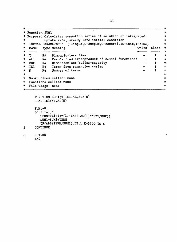
* ______ __ _____ *
* Function SUM1 * * Purpose: Calculates summation series of solution of integrated * * uptake rate, steady-rate initial condition * * FORMAL PARAMETERS: (I-input,0=output,C=control,IN-init,T«time) * * name type meaning units class * * * * T R4 Dimensionless time - I * * AL R4 Zero's from crossproduct of Bessel-functions: - I * * BUF R4 Dimensionless buffer-capacity - I * * TE1 R4 Terms from summation series - I * * N R4 Number of terms - I * * * * Subroutines called: none * * Functions called: none * * File usage: none * * — — *
FUNCTION SUM1(T,TE1,AL,BUF,N) REAL TE1(N),AL(N)
SUM1-0. DO 5 I-l.N
TERM-TE1(I)*(1.-EXP(-AL(I)**2*T/BUF)) SUM1-SUM1+TERM IF(ABS(TERM/SUM1).LT.1.E-5)G0 TO 6
5 CONTINUE
6 RETURN END

34
* *
* Function SUM2 * * Purpose: Calculates summation series of solution of uptake rate, steady-* * rate initial condition * * FORMAL PARAMETERS: (I-input,0-output,Ocontrol,IN-init,T-time) * * name type meaning units class * * * * T R4 Dimensionless time -* AL R4 Zero's from crossproduct of Bessel-functions: -* BUF R4 Dimensionless buffer-capacity -* TE2 R4 Terras from summation series -* N R4 Number of terms -* * * Subroutines called: none * * Functions called: none * * File usage: none * * *
FUNCTION SUM2(T,TE2,AL,BUF,N) REAL TE2(N),AL(N)
SUM2-0. DO 5 I-l.N
TERM-TE2(I)*EXP(-AL(I)**2*T/BUF) SUM2-SUM2+TERM IF(ABS(TERM/SUM2).LT.l.E-5)GO TO 6
5 CONTINUE
6 RETURN END
35
* ___ _*
* Subroutine CUMUP * * Purpose: calculates uptake rate and cumulative uptake in zero-sink * * situation, and their steady-rate approximations as a function * * of time. * * * * FORMAL PARAMETERS: (I-input,0-output,C-control,IN-init,T-time) * * name type meaning units class * * * * NI 14 Number of time-steps - I * * TFAC R4 Ratio between real and dimensionless time day I * * NU R4 Dimensionless flux of water - I * * BUF R4 Buffer capacity - I * * TAUM R4 Dimensionless maximum period of unconstrained - I * * uptake * * TAUNU R4 Dimension less period of unconstrained uptake - I * * UPR R4 Required uptake rate nutrient kg/(ha.day) I * * AL R4 Zero's from crossproduct of Bessel-functions * * TIME R4 Time days 0 * * UP R4 Uptake rate in zero-sink situation kg/(ha.day) 0 * * UPAP R4 Uptake rate in zero-sink situation, kg/(ha.day) 0 * * steady-rate approximation * * TUP R4 Cumulative uptake kg/ha 0 * * TUPAP R4 Cumulative uptake steady-rate approximation kg/ha 0 * * * * Subroutines called: * * TERM: calculates terms of summation series * * * * Functions called: * * SUM1.SUM2: produce values of summation series * * GRNU : Calculates G-function * * * * File usage: none * * • *
SUBROUTINE CUMUP(NI,RHO,TFAC,TAUM,TAUNU,UPR,BUF,TNU, 1 COF.Rl.HSC.CII.DIF,TIME,UP,UPAP,TUP,TUPAP) DIMENSION TIME(30),UP(30),UPAP(30),TUP(30),TUPAP(30) DIMENSION TE1(50),TE2(50),TE3(50),TE4(50),AL(50) REAL NU
NU-TNU/2 CALL TERM(RHO,NU,TE1,TE2,TE3,TE4,50,AL) WRITE(46,*) 'TERM ',(TE4(I),1-1,20)
TAU-TAUNU IF(TAUNU.LT.0.)TAU-0. STEP-(TAUM-TAU)/NI
* — Do 30 over time DO 30 I-l.NI+1
TIM-FLOAT(I-1)*STEP TIME(I)-TFAC*(TAU+TIM)

36
IF(TAUNU.GT.O.)THEN UP(I)-UPR*COF*SUM2(TIM,TE2,AL,BUF,50) UPAP(I)-UPR*EXP(-TIM/(BUF*GRNU(TNU,RHO)))
ELSE UP(I)—4.*HSC*DIF*CII*SUM2(TIM,TE4)AL,BUF,50)/
1 Rl**2*100. UPAP(I)-100.*HSC*DIF*CII/R1**2*(RHO**2-1.)
1 *EXP(-TIM/(BUF*GRNU(TNU,RHO)))/GRNU(TNU,RHO) ENDIF IF(TIM.LE.O.)THEN
TUP(I)-UPR*TFAC*TAU ELSE
IF(TAUNU.GT.O.)THEN TUP(I)-UPR*TFAC*TAU+COF*BUF*UPR*TFAC
1 *SUM1(TIM,TE1,AL,BUF,50) TUPAP(I)-UPR*TFAC*BUF*GRNU(TNU,RHO)*(1.-EXP(-TIM/
1 (BUF*GRNU(TNU,RHO)))) + UPR*TFAC*TAU ELSE TUP(I)-UPR*TFAC*TAU-4.*100.*TFAC*HSC*DIF*CII
1 *BUF*SUM1(TIM,TE3,AL,BUF,50)/R1**2 TUPAP(I)-100.*HSC*DIF*CII/R1**2*(RHO**2-1.)*
1 TFAC*BUF*(l.-EXP(-TIM/(BUF*GRNU(TNU,RHO)))) ENDIF
ENDIF
30 CONTINUE RETURN END
37
* *
* Function GRNU * * Purpose: Calculation of G(nu,rho), (De Willigen & Van Noordwijk, 1987 * * page 130) * * * * FORMAL PARAMETERS: (I-input,0-output.C-control,IN-init,T-time) * * name type meaning units class * * * * TNU R4 2*NU, NU dimensionless flux of water - I * * RHO R4 Dimensionless radius soil cylinder - I * * * * Subroutines called: none * * Functions called: none * * File usage: none * * — . — *
FUNCTION GRNU(TNU,RHO) RH02-RHO*RHO IF(TNU.EQ.0.)THEN
Gl-(l.-3.*RH02)/4. G2-RH02**2*AL0G(RH0)/(RH02-1.) GRNU=(Gl+G2)/2. RETURN
ELSE GNl-(l.-RH02)/2. GN2«RH02*(RH0**TNU-1.)/TNU GN3-RH02*(RHO**TNU-l.)*(TNU/2.+1.)/(TNU*
1 (RHO**(TNU+2.)-l.)) GN4«(1.-RH0**(TNU+4.))*(TNU/2.+1.)/((TNU+4.)*
1 (RH0**(TNU+2.)-l.)) GRNU-(GNl+GN2+GN3+GN4)/(TNU+2.)
END IF RETURN END
SUBROUTINE ZEJYl(X,N,RHO,ORD,TLIM,EPS,ISIG) DIMENSION BJ(2),BY(2),BRJ(2),BRY(2)
DOUBLE PRECISION JNA,JNRA,JN1A,JNIRA.YNA.YNRA.YNIA, $ YN1RA.FA.FAA
PRINT *,'TLIM ',TLIM IP-0 ORD1-ORD+1 PI-3.141592654 S-N X-(S-0.5)*PI/(RHO-1.) TEL-0. SOL-X TEL-TEL+1 IF(TEL.GT.TLIM)GO TO 5 IF(SOL.LE.0.)GO TO 10 RSOL-RHO*SOL CALL BESFRJ(SOL,ORD,ISIG,BJ) CALL BESFRY(SOL,ORD,ISIG,BY) CALL BESFRJ(RSOL,ORD,ISIG,BRJ) CALL BESFRY(RSOL,ORD,ISIG,BRY) JNA-BJ(l) JN1A-BJ(2) YNA-BY(l) YN1A-BY(2) JNRA-BRJ(l) JN1RA«BRJ(2) YNRA-BRY(l) YN1RA-BRY(2)
38
* *
* Subroutine ZEJY1 * * Purpose: calculates the n-th root of: * * Y(0RD+1,RH0*X)*J(0RD,X)-Y(0RD,X)*J(0RD+1,RH0*X) * * J,Y Bessel-functions of first kind, order ORD * * Solution by Newton-raphson iteration, first estimate as given * * in Abramowitz & Stegun , page 374, 9.5.33. * * FORMAL PARAMETERS: (I-input,0=-output,C-control, IN«init,T«time) * * name type meaning units class * * * * N 14 rootnumber * * TLIM R4 maximum number of iterations - I * * EPS R4 required accuracy - I * * X R4 the value of the root 0 * * IP 14 Error indicator 0 * * * * Subroutines called: * * BESFRJ: calculates Bessel function J of fractional order * * BESFRY: calculates Bessel function Y of fractional order * * Functions called: none * * File usage: none * * *

39
DJN—JN1A+0RD/S0L*JNA DYN—YNlA+ORD/SOL*YNlA DJN1R-RHO*(JNRA-ORD1/RSOIAJN1RA) DYN1R-RHO*(YNRA-0RD1/RS0L*YN1RA) FA-JNA*YN1RA-JN1RA*YNA
* PRINT *,'TEL,SOL,FA ',TEL,SOL,FA FAA-YN1RA*DJN+JNA*DYN1R-JN1RA*DYN-YNA*DJN1R X-SOL-FA/FAA IF(ABS((SOL-X)/X).GT.EPS)GO TO 1 RETURN
5 CONTINUE PRINT 100 IP-2 RETURN
10 PRINT 101,TEL,SOL IP-3 RETURN
100 FORMAT(1H0,'TOO MANY ITERATIONS IN ZEJYl') 101 FORMAT(1HO,'AFTER',F5.0,IX,'ITERATION, NEGATIVE ARG:
11PD15.5)
END

40
* *
* Subroutine: BESFRJ * * Purpose: calculates bessel-functions first kind * * for argument x and (fractional) orders alph and alph+1 * * *
* FORMAL PARAMETERS: (I-input,0-output,C-control,IN-init,T-time) * * name type meaning units class * * * * X R4 argument of Besselfunction - I * * ALPH R4 order of Besselfunction - I * * ISIG R4 required significant digits - I * * BJ R4 contains the values of J(ALPH,X), J(ALPH+1,X) 0 * * * * Subroutines called: * * BESJN from CERNLIB * * Functions called: none * * File usage: none * * *
SUBROUTINE BESFRJ(X,ALPH,ISIG,BJ) DIMENSION BBJ(2),BJ(1)
C IF(ALPH.LT.0.)GO TO 5 NNN-ALPH ALP-ALPH-NNN CALL BESJN(X,ALP,NNN,ISIG,BBJ) BJ(1)-BBJ(1) BJ(2)-BBJ(2) RETURN
5 CONTINUE NNN-ALPH-1. ALP-ALPH-NNN CALL BESJN(X,ALP,NNN,ISIG,BBJ) BJ(1)-BBJ(2) BJ(2)-BBJ(1) RETURN END

41
* Subroutine BESFRY * Purpose: calculates modified bessel-functions first kind * for argument x and (fractional) orders alph and alph+1
* X R4 argument of Besselfunction - I * ALPH R4 order of Besselfunction - I * ISIG R4 required significant digits - 1 * BY R4 contains the values of Y(ALPH,X), Y(ALPH+1,X) 0 *
* Subroutines called: * BESFRJ * Functions called: none * File usage: none * _ — — — —
SUBROUTINE BESFRY(X,ALPH,ISIG,BY) DIMENSION BY(1),BBJ(2),BBMJ(2) PI-3.1415926535 CO-COS(ALPH*PI) SI-SIN(ALPH*PI) ALP—ALPH CALL BESFRJ(X,ALP,ISIG,BBMJ) CALL BESFRJ(X,ALPH,ISIG,BBJ) BY(1)-(BBJ(1)*C0-BBMJ(1))/SI BY(2)—(2./(PI*X)-BBJ(2)*BY(l))/BBJ(l)
1 CONTINUE RETURN END

42
APPENDIX II. Numerical solution of radial flow of water to a plant root.
Background
The program solves the following partial differential equation,
£ - hl^r <AII-1)
with boundary conditions:
r - P , -^ " ° (AII-2) Br
and e i t he r :
r - 1 , L | £ J - constant - q (AII-3a)
or:
r - 1 , B - constant - 8rs (AII-3b)
The initial condition is simply :
t - 0, 6 - constant - 8\ (AII-4)
The meaning of the symbols can be found in table 1 in the main text. Equation (AII-1) is Richard's equation in cylindrical coordinates.
Before discretisizing the partial differential equation (AII-1), the hollow cylinder with inner radius 1 and outer radius p, is transformed to a rectangle by the transformation:
x - lnr (AII-5)
This transforms (AII-l)-(AII-3) into resp.:
«2,£ - &•£ <AII-6>
x - lnp , 1*1-0, (AII-7) dx
x - 0, 11 - q (AII-8a) dx
and

43
o, e - ers
(AII-8b)
Equation (AII-6) is discretized by dividing the region 0 < x < lnp into a number of control-volumes and integrating of (AII-6) over the control-colume and a finite time-step At (Patankar, 1980) following a complete implicit scheme. This leads to a set of n equations in the n unknown 9, where n is the number of control volumes. These equations have the form:
ai6i - bi6Ul + <:,•*,•_! + d,- (AII-9)
where
1 Ax* ' "AF
e2(i-l)AX „2(i-l)AX „
a,- - bj + Cj + sinh(Ax) _ , a,- - sinh(Ax)_ 0"
Ax is the thickness of the control-volumes, At the time-step, D,- and D,.! the average diffusivities at the boundaries of control-volume i and i+1, resp i-1 and i. It is to be understood that all values of 6 are the new unknown values at time t+At except where the superscript ° is used. The coefficients a.b.c and have special values at the boundaries, where i-1 resp i-=n. For i=l (x-0), if condition of constant flux (AII-8a) is used:
. . (e*»-l) +~PT b _~E± 1 IKE~ Ax ' x Ax
Ci-0, d^-q* SfJ^lol ,
whereas when for constant watercontent (AII-8b)
ax - 1, bx- 0, cx - 0, dx - 8rs.
For i-n (x-lnp)
( 2 . e2(n-l)AX - AX)
*" IKE b" °
'n -ST' n IKE °n

kk
The solution of the discretization eqations (AII-9) is found by the TDMA algorithm (Patankar, 1980).
Program
The relation between the subroutines is given in the diagram in Figure AII-1. The core of the program is formed by the subroutine SOLVE wherein the discretization equations are solved. Due to the nonlinear relation between the diffusivity and the water content the solution is found by iteration. If necessary underrelaxation can be used to avoid divergence (Patankar, 1980, Ch 4. page 67).
Relational diagram of subroutines in FLROOT
-Q INIT ) (WATERC)
(VLROOTJ 1
MOFILP 0
GEOMR 0 -/TIMEST') AVDIF X FDIF
TDMA
-Q SOLVE)—(^COEFF)
<
k OUTP
UPDAT -C™£>
; >
The relation between diffusivity and water content is as proposed by Van Genuchten (1980):
D-K*<6"\sJw'l-J M1-**)" " (0Sat-0r)<*n-
where
8 - 9r W - m -
"sat ~ "r 1 - 1
n
(AII-10)

45
This is calculated in the function FDIF, and is used in the function FLPL which calculates the integral give in (11). The numerical integration is performed by the function GAUSS (not shown) which is taken from CERNLIB Lindelof, 1981).

46
* *
* Program FLROOT * * Purpose : Calculation of flow of water towards a root. * * The geometry is a hollow cylinder representing the soil around* * the root. Boundary conditions are: constant flux, or constant * * water-content at the root surface (the inner cylinder) and * * zero-flux at the outer cylinder. The partial differential * * equation is solved by completely implicit finite difference * * scheme, as described in S.V. Patankar, 1980, Numerical heat * * transfer and fluid flow. * * The flow is also calculated with an analytical function, * * based on the steady-rate approximation (De Willigen and * * Van Noordwijk, 1987, Roots, plant production and nutrient use * * efficiency page 149, (9.73)). * * * * The mutual relations between matric potential, water content, * * and hydraulic conductivity are given by Van Genuchten functions. * * * * SUBROUTINES called: * * MOFILP: organizes input * * INIT: initializes watercontent * * GEOMR: calculates geometry, thickness control-volumes etc. * * SOLVE: solves the discretization equations * * UPDAT: updates watercontent, calculate totals, averages, etc. * * OUTP: organizes the output * * * * FILE usage: * * 1. input from screen (format: soilname.DAT),unit 40, * * contains soil and root data (I) * * 2. C0NTR.DAT, unit 40, contains data that control boundary * * conditions, iteration, relaxation (I) * * 3. soilname.PET, unit 41, main outputfile (0) * * 4. soilname.PLO, unit 48, plotfile with data (0) * * * * *
DIMENSION G(30),C(30),WCN(30),DIFDN(30) DIMENSION A(30),X(30),B(30),D(30),WCOL(30) DIMENSION USTR(30),WCSTR(30),DW(30)
REAL KS,M,N,L REAL U(30),R(30),LRV REAL WC(30),DWCDT(30),DIFD(30) CHARACTER*20 NAME,INP,0UTF LOGICAL MODE
COMMON /FDIF1 / WCSAT,WCR,M,N,L,ALPH,KS
DATA FLB/1./
* INITIAL *

47
PI-ATAN(1.)*4. TW0PI-2.*PI
input PRINT *,'SOILNAME?* READ(*,100) NAME
OPEN (UNIT-40,FILE-NAME) File with soil and root-data is opened
Outputfile is opened I - INDEX (NAME,'.') IF (I.EQ.O) I - INDEX (NAME,' ') NAME(I:I+3) - '.PET' OPEN (UNIT-41,FILE-NAME)
NAME(I:I+3)-'.PLC 0PEN(UNIT-48,FILE=NAME)
Plotfile is opened
Reading of soil and root data CALL MOFILP(40) READ(40,100) NAME CALL M0FILP(40) READ(40,*) WCSAT.WCR.WCMIN.WCREF.PLIM.PMIN PRINT *,'WCSAT,WCR,WCMIN,WCREF,PLIM '.WCSAT.WCR.WCMIN.WCREF PLIM CALL MOFILP(40) READ(40,*) KS.N.L.ALPH M-l.-l./N CALL MOFILP(40) READ(40,*) LRV.RO.HSC CALL MOFILP(40) READ(40,*) EVAP CALL MOFILP(40) READ(40,*) WCI CALL MOFILP(40) READ(40,*) IR CLOSE(40)
SOILNAME.DAT is closed
C0NTR.DAT is opened OPEN(FILE-'CONTR.DAT'.UNIT-40)
reading control data CALL M0FILP(40) READ (40,*) TFAC
* maximum change watercontent * over time-step
CALL MOFILP(40) READ (40,*) CHMAX
* iteration tolerance CALL MOFILP(40)

48
READ (40,*) EPS * relaxation factor
CALL MOFILP(40) READ (40,*) RELF
* CURS < 0 , water content at root surface * constant
CALL MOFILP(40) READ (40,*) CWRS
* read waterpotential root * surface
IF(CWRS.LT.O.)THEN CALL MOFILP(40) READ (40,*) PRS FLB—1.
ELSE ENDIF
* Close C0NTR.DAT CLOSE(40)
* — — End input * Initialisation
CALL 1NIT(IR, LRV,HSC,R0,UCI,PLIM,EVAP,FLB,PRS , 1 Rl,SUMWI,RHO,ETA,WCLIM,QT,RAT,WC,WCAPP)
Reading time data from screen TMAX-SUMWI/(PI*R1**2*EVAP) PRINT *,'MAXIMUM EXTRACTION TIME IN DAYS ',TMAX PRINT *,'GIVE FINTIM IN DAYS' READ *,FINTIM PRINT *,'PRINT-INTERVAL IN DAYS' READ +.PRDEL
Geometry CALL GEOMR(IR,RHO,X,R,DX,DX2)
PRDELT-PRDEL*RAT IP-0 T-0 WRITE(41,*) 'FINTIM,DELT.DT '.FINTIM,DELT.DT
DELT-.l FIT-0 TRPAR-1. WCAPP-WCI
DYNAMIC
10 CONTINUE
IF(WC(1).LE.WCLIM.AND.FLB.GT.0.)THEN FLB—1.

49
WRITE(41,*) 'TIME- '.TIME,' WC(1).LE.WCLIM' PRINT 101,TIME,DELT PRINT 102,(WC(K),K»1,IR) CALL OUTP(IR,R,R0,HSC,Rl,T,TIME,DELT,WCN,WC,DWCDT,DIFD,
1 BAL,RUPW,RUPWSR,CUPW,CUPWSR,WCAV,WCAPP) ENDIF
Check if time exceeds fintim IF(TIME.GE.FINTIM)GO TO 20
Check if output should be written IF(TIME.GE.(IP*PRDEL))THEN
IP-IP+1 CALL OUTP(IR,R,R0,HSC,Rl,T,TIME,DELT,WCN,WC,DWCDT,DIFD,
1 BAL,RUPW,RUPWSR,CUPW,CUPWSR,WCAV,WCAPP) ENDIF
CALL SOLVE(IR,WC,WCN,DELT,DX,RHO,QT,FLB,RELF,EPS,WCLIM, 1 DIFD)
CALL UPDAT(IR.WC,WCN,WCLIM,R,R0,R1,HSC,DELT,T, 1 DWCDT,RUPW,RUPWSR,CUPWSR,CUPW,BAL,WCAV,WCAPP)
TIME-T*(R0*R0)
CALL TIMEST(DELT,FLB,TFAC,CHMAX,WC,DWCDT,PRDELT)
GO TO 10
20 CONTINUE WRITE(41,*) ' TIME .GE. FINTIM ' CALL OUTP(IR,R,R0,HSC,R1,T,TIME,DELT,WCN,WC,DWCDT,DIFD,
1 BAL,RUPW,RUPWSR,CUPW,CUPWSR,WCAV,WCAPP) STOP
100 FORMAT (A20) 101 FORMAT(1H0,'TIME -'1PE15.5,1X,'DELT -'1PE15.5) 102 FORMAT(1HO,/13X,'WC'/(1PE15.5))
END
50
*_ * * * * * * * * * * * * * * * * * * * * * * * * * * * * * * * *-
Subroutine INIT Purpose: Initialisation of watercontent, calculation of parameters FORMAL PARAMETERS: (I-input,0-output,C-control,IN-init,T-time) name type meaning units class
LRV HSC R0 WCI PLIM EVAP FLB
PRS Rl RHO SUMWI ETA WCLIM QT WC WCAPP
R4 R4 R4 R4 R4 R4 R4
R4 R4 R4 R4 R4 R4 R4 R4 R4
Root length density Root lenght Root radius Initial water content Limiting value matric potential Required transpiration Parameter that controls boundary condition at root surface. FLB>0 constant flux, FLB<0 constant watercontent Matric potential at root surface Radius soil cylinder Dimensionless radius soil cylinder Initial total amount of water in soil Dimensionless root lenght limiting value water content Required uptake rate of water by root Water content Water content calculated by steady-rate approximation
cm/cm3 cm cm
cm cm/day
cm cm
cm3
cm2/day
I 0 0 0 0 0 0 0 0
Subroutines called: none
Functions called: WATERC: calculates water content as a function of matric potential
File usage: soilname.PET
-* * * * * *
* * * * * * * * * * * * * * * * * * * * * * * * *
SUBROUTINE INIT(IR,LRV,HSC,R0,WCI,PLIM,EVAP,FLB,PRS, Rl,SUMWI,RHO,ETA,WCLIM,QT,RAT,WC,WCAPP)
DIMENSION WC(30) REAL M,N,L,KS,LRV COMMON /FDIF1 / WCSAT,WCR,M,N,L,ALPH,KS
PI-4.*ATAN(1.) R1-1./SQRT(PI*LRV) SUMWI-PI*(R1*R1-R0*R0)*HSC*WCI RHO-R1/R0 ETA-HSC/RO WCLIM-WATERC(PLIM,WCSAT,WCR,N,ALPH) QT-RH0**2/(2.*ETA)*EVAP*R0 RAT«l./(Ru*R0)
initialisation OF WATER CONTENT DO 30 K-2.IR+1
WC(K)-WCI

51
30 CONTINUE IF(FLB.GT.O.)THEN
WC(1)-WCI ELSE
WC(1)-WATERC(PRS,WCSAT,WCR,N,ALPH) ENDIF WCAPP-WCI
* initial output WRITE(41,100) LRV.EVAP.RHO,ALPH,QT,RAT PRINT 100,LRV.EVAP.RHO,ALPH,QT,RAT PRINT 101.SUMWI WRITE(41,101) SUMWI RETURN
100 FORMAT(IX,//,IX,'ROOT-DENSITY CM-2:'F5.1/ 1 IX,'EVAPOTRANSPIRATION CM/DAY :'F6.2/ 2 lX.'RHO ;'1PE15.5/ 3 IX,'ALPH :'1PE15.5/1X, 4 lX.'DIMENSIONLESS UPTAKE QT:'1PE15.5/ 5 IX,'RATIO DIMENSIONLESS TIME AND REAL TIME:'1PE15.5)
101 FORMAT(IX,'SUMWI-'1PE15.5)
END

52
* *
* Subroutine: SOLVE * * Purpose: construction of coefficient-matrix of discretisized equations * * and solving the equations by TDMA * * FORMAL PARAMETERS: (I-input.O-output.C-control,IN-init,T-time) * * name type meaning units class * * * * WC R4 Water content - I * * WCN R4 New values of water content - 1,0 * * DELT R4 Time step in scaled units day/cm2 I * * DX R4 Thickness control-volume - I * * RHO R4 Dimensionless radius soil cylinder - I * * QT R4 Uptake rate of water by root cm2/day I * * FLB R4 Parameter that controls boundary condition I * * at root surface. FLB>0 constant flux, * * FLB<0 constant watercontent * * RELF R4 Relaxation factor - I * * EPS R4 Convergence criterion for iteration - I * * DIFD R4 Average diffusivity at face control volume - 0 * * WCLIM R4 limiting value water content 0 * * * * Subroutines called: * * COEFF: calculates coefficients discretization equations * * TDMA : solves discrtization equations * * * * Functions called: * * AVDIF: calculates average diffusivity at interface * * two control-volumes * * File usage: none * * * * *
SUBROUTINE SOLVE(IR,WC,WCN,DELT,DX,RHO,QT,FLB,RELF,EPS,WCLIM, 1 DIFD)
DIMENSION WC(30),WCN(30) DIMENSION WCOL(30),DIFD(30),A(30),B(30),C(30),D(30),DIFDN(30)
10 CONTINUE * average diffusivities are calculated * old values of WC stored in WCOL
DO 20 K-l.IR-1 DIFD(K)-AVDIF(WC(K),WC(K+1),.FALSE.) WC0L(K)-WC(K)
20 CONTINUE WCOL(IR)-WC(IR)
* tentative new values of WC (WCN) calculated * no relaxation
CALL C0EFF(IR,A,B,C,D,WC,DIFD)1.,DX,RH0,DELT,QT,FLB,WC(1), 1 WCOL,RELF,0)
CALL TDMA(IR,A,B,C,D,WCN)

53
iterative search for better new values of WC DO 50 IT-1,10
IF(WCN(l).LT.0.)GO TO 60 DO 30 K-l.IR-1
TRPAR-1. IF(WCN(K).LT.WCLIM)THEN
TRPAR—1. ENDIF DIFDN(K)-AVDIF(WCN(K),WCN(K+1),.FALSE.)
30 CONTINUE * criterion of convergence is relative * — — difference between consecutive values of * — — diffusivity at first or second gridpoint
DIFCRT-(DIFDN(1)-DIFD(1))/DIFD(1) IF(FLB.LT.0.)DIFCRT-(DIFDN(2)-DIFD(2))/DIFD(2) IF(ABS(DIFCRT).LT.EPS)THEN GO TO 70
ELSE CALL C0EFF(IR,A,B,C,D,WC,DIFDN,1.,DX,RHO,DELT,QT,FLB,
1 WC(1),WC0L,RELF,IT) CALL TDMA(IR,A,B,C,D,WCN) DO 40 K-l.IR
TRPAR-1. IF(WCN(K).LT.WCLIM)THEN
TRPAR—1. ENDIF DIFD(K)-DIFDN(K) WCOL(K)-WCN(K)
40
50
60
.L.
70
CONTINUE ENDIF
CONTINUE
DELT-DELT/2. GO TO 10
CONTINUE
RETURN END
— end of iteration

54
* * * * * * * * * * * * * * * * * * * * * * * * *-
Function FLPL * Purpose: Calculation of matric flux potential as integral of diffusivity*
over watercontent
FORMAL PARAMETERS: (I-input,0-output,C-control,IN=init,T-time) name type meaning units class
ALPH WCR KS
R4 R4 R4
water content Watercontent at saturation parameter from conductivity-watercontent relation parameter residual water content saturated conductivity
ml/cm3 ml/cm3
cm-1 ml/cra3 cm/day
I I I
I I I
Subroutines called: none
Functions called : GAUSS: a function from CERNLIB which performs numerical
integration according to Gauss' method. FDIF: calculates diffusivity as a function of water content.
File usage: none
REAL FUNCTION FLPL(WC) REAL KS.M.N.L COMMON /FDIF1/ WCSAT,WCR,M.N.L,ALPH,KS EXTERNAL FDIF
FLPL-GAUSS(FDIF,WC,0.99*WCSAT,.001)
RETURN END
55
* *
* FUNCTION WATERC * * Purpose : Calculation of watercontent by hydraulic head Van Genuchten * * function. * * FORMAL PARAMETERS: (I-input,0-output,C-control,IN-init,T-time) * * name type meaning units class * * * * PRES R4 hydraulic head cm I * * WCSAT R4 Watercontent at saturation ml/cm3 I * * N R4 parameter from conductivity-watercontent - I * * relation * * ALPH R4 parameter cm-1 I * * WCR R4 residual water content ml/cm3 I * * WATERC R4 watercontent ml/cm3 0 * * * * Subroutines/functions called: none. * * * * File usage: none * * * * — — — *
FUNCTION WATERC(PRES,WCSAT,WCR,N,ALPH) REAL M,N M-l.-l./N IF(PRES.LE.O.)THEN
TRPAR—1 END IF HELP-(1.+(ALPH*PRES)**N) IF(HELP.LE.O.)THEN
TRPAR—1 ELSE ENDIF WATERC-(WCSAT-WCR)*(1.+(ALPH*PRES)**N)**(-M)+WCR RETURN END
56
* *
* Function FDIF * * Purpose: Calculation of diffusivity from watercontent * * FORMAL PARAMETERS: (I-input,0-output,C-control,IN=-init,T-time) * * name type meaning units class * * —: * * WCSAT R4 Watercontent at saturation ml/cm3 I * * N R4 parameter from conductivity-watercontent - I * * relation * * ALPH R4 parameter cm-1 I * * WCR R4 residual water content ml/cm3 I * * FDIF R4 Diffusivity cm2/day * * * * SUBROUTINES called: none * * FUNCTIONS called: none * * FILE usage:none * * *
FUNCTION FDIF(WC) REAL KS.M.N.L COMMON /FDIF1/ WCSAT,WCR,M,N,L,ALPH,KS
W-(WC-WCR)/(WCSAT-WCR) M-l.-l./N TRPAR-1. IF(W.LT.O.)THEN
TRPAR—1. ENDIF WL-W**(-1./M) TRPAR-1 IF(WL.LE.1.)THEN
TRPAR—1 ENDIF FDIF-KS*W**L/((WCSAT-WCR)*ALPH*N)*(WL-1.)**(-M)*
1 (l.-(l.-W**(l./M))**M)**2 RETURN END FUNCTION FG(R) FG-0.5*((l-3.*R**2)/4.+R**4*ALOG(R)/(R**2-l)) RETURN END

57
* — _____ _ _ _ _ *
* Subroutine TIMEST * * Purpose: calculation of time step DELT * * * * FORMAL PARAMETERS: (I-input,0-output,C-control,IN=-init,T-time) * * name type meaning units class * *
* DWCDT R4 rate of change of WC cm2/day I * PRDELT R4 print-interval in scaled units day/cm2 I *
* FILE usage: none * —
* DELT R4 timestep in scaled units day/cm2 1,0 * * TFAC R4 multiplying factor, if possible DELT is I * * increased by TFAC * * CHMAX R4 permitted maximum relative change in - I * * watercontent * * WC R4 watercontent I *
* * *
* Subroutines/Functions called: none *
SUBROUTINE TIMEST(DELT,FLB,TFAC,CHMAX,WC,DWCDT,PRDELT) DIMENSION WC(30),DWCDT(30)
IF(FLB.GT.O.)THEN DCH-CHMAX*WC(1)/ABS(DWCDT(1))
ELSE DCH-CHMAX*WC(2)/ABS(DWCDT(2))
ENDIF DELT2-DELT*TFAC DELT-AMIN1(DCH,PRDELT,DELT2)
RETURN END
-*

58
* * * * * * * * * * * * * * * * * * * * * * * * * * * * * * * * *-
Subroutine: UPDAT Purpose: Updating of watercontent, time, total amount of water in soil,
decrease of total water, transpiration by steady-rate approximation
FORMAL PARAMETERS: (I-input,0-output,C-control,IN-init.T-time) name type meaning units class
R RO HSC Rl wc WCN DWCDT DELT RHO WCLIM RUPW CUPW R CUPWSR R4 BAL R4 WCAPP R4
WCAV R4
R4 R4 R4 R4 R4 R4 R4 R4 R4 R4 R4 R4
Dimensionless radial coordinate Radius root Root length Radius soil cylinder Water content New values of water content Rate of change of water content timestep in scaled units Dimensionless radius soil cylinder water content at root surface Rate of uptake of water Cumulative water uptake As RUPW and CUPW but calculated with steady-rate approximation Balance of water in soil Average water content calculated by steady-rate approximation Average water content
cm cm cm
cm2/day day/cm2
cm/day cm
cm/day cm cm
Subroutines called: none.
Functions called: FLPL: calculates matric flux potential as a
water content function of
,0
-* * * * * * * * * * * * * * * * * * * * * * * * * * * * * * * * *
-*
SUBROUTINE UPDAT(IR.WC,WCN,WCLIM,R,R0,R1,HSC,DELT,T, 1 DWCDT,RUPW,RUPWSR,CUPWSR,CUPW,BAL,WCAV,WCAPP)
DIMENSION WC(30),WCN(30),DWCDT(30),R(30),USTR(30) LOGICAL INIT DATA INIT/.FALSE./
IF(.NOT.INIT) THEN RHO-R1/R0 ETA-HSC/RO PI-4.*ATAN(1.) INIT-.TRUE. SUMWI-(R1*R1-R0*R0)*HSC*WC(2)/Rl**2
ENDIF

59
calculation of DWC/DT DO 10 K-l.IR
DWCDT(K)-(WCN(K)-WC(K))/DELT 10 CONTINUE
* SUMW total water in soil cylinder cm * RUPW rate of decrease of water cm/day
SUMW-0. RUPW-0. DO 20 K-l.IR-1
SUMW-SUMW+ 1 (R(K+l)-R(K))*(R(K+l)*WC(K+l)+R(K)*WC(K))/2.
RUPW-RUPW+ 1 (R(K+l)-R(K))*(R(K+l)*DWCDT(K+l)+R(K)*DWCDT(K))/2
20 CONTINUE SUMW-2.*HSC*R0**2*SUMW/R1**2 RUPW—2. *HSC*RUPW/R1**2 BAL-SUMW+CUPW-SUMWI
WCAV average water content WCAV-SUMW*R1**2/(HSC*(Rl**2-R0**2)) USTR(1)-FLPL(WC(1)) UAVAPP-FLPL(WCAPP)
* — RUPWSR water uptake according to steady-rate * approximation cm/day
RUPWSR-2.*HSC/Rl**2*(USTR(l)-UAVAPP)*(RHO**2-l.)/(2.*FG(RHO))
IF(WCN(1).LE.WCLIM.AND. WC(1).GT.WCLIM)THEN DELT-AMIN1(DELT,(WCLIM-WC(1))/DWCDT(1)) TRPAR—1.
ENDIF
* Updating of WC DO 30 K-l.IR
WC(K)-WC(K)+DWCDT(K)*DELT TPAR-1. IF(WC(K).LT.WCLIM)THEN
TRPAR—1. ENDIF
30 CONTINUE
T-T+DELT
CUPW-CUPW+RUPW*DELT*R0**2 CUPWSR-CUPWSR+RUPWSR*DELT*R0**2 WCAPP-WCAPP-RUPWSR*DELT*R0**2*R1**2/(HSC*(R1**2-R0**2)) RETURN END

WRITE(41,100) IR.DR PRINT 100.IR.DR
WRITE(41,101) (R(K),K-1,IR) PRINT 101,(R(K),K-1,IR)
RETURN
100 FORMAT(1H0,I3,IX,'POINTS IN R-DIRECTION'/ 3/lX,'DR-'lPE15.5)
101 FORMAT(1HO,'R-'1P5E15.5)
END
60
* * * Subroutine GEOMR * * Purpose: calculation of position of gridpoints both in transformed and * * untransformed coordinates * * Note: Gridpoints equidistant in transformed region, distances between * * gridpoints geometrically increasing in untransformed cylindrical region.* * * * FORMAL PARAMETERS: (I-input,0-output,C-control.IN-init,T-time) * * name type meaning units class * * * * IR 14 Number of gridpoints - I * * RHO R4 Dimensionless radius soil cylinder - I * * R R4 Radial coordinate gridpoint - 0 * * X R4 Coordinate of gridpoint in transformed region: - 0 * * X - Ln(R) * * DX R4 Distance between gridpoints in transformed region * * * * Subroutine/Finstions called: none * * * * File usage: Coordinates gridpoints wriiten to file soilname.PET * * * * *
SUBROUTINE GEOMR(IR,RHO,X.R.DX.DX2) DIMENSION X(30),R(30)
DX-AL0G(RH0)/(IR-1) DX2-DX*DX R(l)-1. X(l)-0. DO 10 K-2.IR
X(K)-X(K-1)+DX R(K)-EXP(X(K))
10 CONTINUE

61
* _ — _ _ *
* Function: AVDIF * * Purpose: calculates harmonic or arithmetic average of diffusivities, * * with equal weights * * FORMAL PARAMETERS: (I-input,0-output,C-control,IN-init,T-time) * * name type meaning units class * * * * XI,X2 RA dummies, representing watercontent - I * * MODE L If .true, harmonic average, else arithmetic * * * * Subroutines ca l led : none * *
* * -
FUNCTION AVDIF(X1,X2,M0DE) LOGICAL MODE Dl-FDIF(Xl) D2-FDIF(X2) IF(MODE) THEN
AVDIF-2*D1*D2/(D1+D2) ELSE
AVDIF-(Dl+D2)/2. ENDIF RETURN END
* * Functions called: * * FDIF: calculates diffusivity as a function of water content * * ' * * File usage: none *

62
* *
* Subroutine COEFF * * Purpose: calculation of coefficients of the discretization equations. * * These are of the form: * * A(I)*T(I)-B(I)*T(I-H) + C(I)*T(I-1) + D(I), where T(I) is the * * value of the dependent variable at gridpoint I. * * * * FORMAL PARAMETERS: (I-input,0-output,C-control,IN«init,T-time) * * name type meaning units class * * — * * N 14 Number of gridpoints - I * * A.B.C.D R4 Coefficients 0 * * T R4 Dummy denoting the dependent variable * * FM R4 If FM-1 scheme completely implicit, FM=0 I * * scheme completely explicit * DX R4 distance between gridpoints - I * RHO R4 dimensionless radius soil cylinder - I * DT R4 timestep I * Q R4 uptake rate * FLB R4 Parameter that controls boundary condition I * * at root surface. FLB>0 constant flux, * * FLB<0 constant watercontent * * WCLIM R4 water content at root surface - I * * TO R4 Values of T at preceding time-step I * * RELF R4 Relaxation factor I * * IT R4 Controls relaxation, if IT >1 relaxation - I * * * * Subroutines/functions called: none * * * * File usage: none * * * * *
SUBROUTINE COEFF(N,A,B,C,D,T,DIF,FM,DX,RHO,DT,Q,FLB,WCLIM, 1 TO,RELF,IT) DIMENSION A(30),B(30),C(30),D(30),T(30),TO(30),DIF(30) EMFM-l.-FM BETA«(EXP(DX)-EXP(-DX))/2.
DO 5 1-2,N-l AE-DIF(I)/DX AW-DIF(I-1)/DX AOP-BETA*EXP(2.*(FLOAT(I)-1.)*DX)/DT AI-(FM*AE+FM*AW+AOP)
B(I)-FM*AE C(I)-FM*AW DI-AE*EMFM*T(I+1) + AW*EMFM*T(I-1) +
1 (AOP-EMFM*AE-EMFM*AW)*T(I)
63
IF(IT.LE.1)THEN A(I)-AI D(I)-DI
ELSE A(I)-AI/RELF D(I)-DI+(1.-RELF)*A(I)*T0(I)
END IF
CONTINUE
IF(FLB.GT.O.)THEN Al«((EXP(DX)-l.)/(2.*DT)+DIF(l)*FM/DX) B(1)-DIF(1)*FM/DX C(l)-0. D1-DIF(1)*EMFM*(T(2)-T(1))/DX - Q +
1 (EXP(DX)-1.)/(2.*DT)*T(1)
IF(IT.LE.1)THEN A(1)-A1 D(1)-D1
ELSE A(1)-A1/RELF D(1)-D1+(1.-RELF)*A(1)*T0(1)
END IF
ELSE A(l)-1. B(l)-0. C(l)-0. D(1)-WCLIM
ENDIF
AN-((RHO**2-EXP(2.*FLOAT(N-l)*DX-DX))/(2.*DT)+ 1 DIF(N-1)*FM/DX) B(N)-0. C(N)-DIF(N-1)*FM/DX DN—DIF(N-1)*EMFM*(T(N)-T(N-1))/DX +
1 (RHO**2-EXP(2.*FLOAT(N-l)*DX-DX))/(2.*DT)*T(N)
IF(IT.LE.1)THEN A(N)-AN D(N)-DN
ELSE A(N)-AN/RELF D(N)-DN+(l.-RELF)*A(N)*TO(N)
ENDIF
RETURN END

64
* *
* Subroutine TDMA * * Purpose: solves the discretization equations * * * * FORMAL PARAMETERS: (I=input,0-output,C=control,IN=-init,T-time) * * name type meaning units class * * * * N 14 Number of gridpoints - I * * A,B,C,D R4 Coefficients I * * TE R4 Dummy denoting the dependent variable 0 * * * * Subroutines/Functions called: none * * * * File usage: none * * * * *
SUBROUTINE TDMA(N,A,B,C,D,TE) DIMENSION A(30),B(30),C(30),D(30),TE(30) REAL P(50),Q(50) P(l)-B(l)/A(l) Q(l)-D(l)/A(l) DO 5 1-2,N
DEN0M-A(I)-C(I)*P(I-1) P(I)-B(I)/DEN0M Q(I)-(D(I)+C(I)*Q(I-1))/DEN0M
5 CONTINUE TE(N)-Q(N) DO 10 I-N-1,1,-1
TE(I)-P(I)*TE(I+1)+Q(I) 10 CONTINUE
RETURN END

65
*-* * * * * * * * * * * * * * * * * * * * * * * * * * * * * * * * * * * * *-
Subroutine OUTP Purpose: organizes output
FORMAL PARAMETERS: (I-input,0-output,C-controlfIN-init,T-time) name type meaning units class
IR 14 R R4 RO R4 HSC R4 Rl R4 T R4 TIME R4 DELT R4 WC R4 WCN R4 DWCDT R4 BAL R4 RUPW R4 CUPW R4 RUPWSR R4 CUPWSR R4 WCAV R4 WCAPP R4
Number of gridpoints Dimensionless radial coordinate Radius root Root length Radius soil cylinder Time in scaled units Time in absolute units Time step in scaled units Water content New values of water content Rate of change of water content Balance of water in soil Rate of uptake of water Cumulative water uptake As RUPW and CUPW but calculated with steady-rate approximation Average water content Average water content calculated by steady-rate approximation
I I
cm I cm I cm I
day/cm2 I day I day/cm2 I
I I
cm2/day I cm I cm/day I cm I cm/day I cm I
I I
Subroutines called: none
Functions called: FLPL: calculates matric flux potential as a function of
water content
File usage: detailed output written to unit 41, soilname.PET
Plot-output written to soilname.PLO
SUBROUTINE OUTP(IR,R.RO,HSC,Rl.T,TIME,DELT.WCN.WC,DWCDT,DIFD, L BAL,RUPW,RUPWSR,CUPW,CUPWSR,WCAV,WCAPP)
DIMENSION WCN(30),WC(30),DWCDT(30),DIFD(30) DIMENSION USTR(30),WCSTR(30),U(30),R(30) REAL KS.M.N.L
RHO=R1/R0 ETA-HSC/RO
-* * * * * * * * * * * * * * * * * * * * * * * * * * * * * * * * * * * * *
-*
DO 5 I-l.IR U(I)-FLPL(WC(I))
U(I) matric flux potential

66
USUM-0. DO 10 K-l.IR-1
USUM-USUM+ 1 (R(K+l)-R(K))*(R(K+l)*U(K+l)+R(K)*U(K))/2.
10 CONTINUE QT-RHO**2/(2.*ETA)*RUPW*RO
UAVAPP-FLPL(WCAPP) USUM-2.*HSC*R0**2*USUM/R1**2 UAV-USUM*R1**2/(HSC*(R1**2-R0**2)) USTR(1)-FLPL(WC(1))
* USTR(I) matric flux potential calculated with * steady-rate approximation
DO 20 K-2.IR USTR(K)-USTR(1)+QT*
1 ((R(K)**2-l.)/(2.*(RHO**2-l.))-2 RHO**2*ALOG(R(K))/(RHO**2-l.))
20 CONTINUE
IF(TIME.EQ.O.)THEN WRITE(48,100)
END IF
WRITE(41,101) T,TIME,DELT,BAL,WCAV,WCAPP PRINT 101,T,TIME,DELT,SUMW,BAL,WCAV,WCAPP WRITE(41,102) (R(K),WC(K),DWCDT(K),WCN(K),
1 DIFD(K),K-1,IR) WRITE(41,103) (R(K),U(K),USTR(K),K-1,IR) WRITE(41,*) WRITE(41,*) 'UAV - ',UAV,' UAVAPP - '.UAVAPP WRITE (41,*) 'CUPW - '.CUPW,' CUPWSR - '.CUPWSR WRITE(48,104) TIME,RUPW.RUPWSR,CUPW,CUPWSR RETURN
100 FORMAT(IX,1IX,'TIME',10X,'RUPW',10X,'RUPWSR',5X,'CUPW', 1 4X,'CUPWSR')
101 FORMAT(//10X,'T-'1PE15.5,2X,'REAL TIME-'1PE15.5, 1 1X,'DELT-'1PE15.5/ 2 1X,'BAL-'1PE15.5, 3 /lX.'WCAV -'1PE15.5,1X,'WCAPP -'1PE15.5)
102 F0RMAT(/ 1 1X,14X,'R',13X,'WC,10X,'DWCDT',12X,*WCN' 2 .HX.'DIFD'/ 3 (1X.1P5E15.5))
103 F0RMAT(/1X,14X,'R',14X,'U',11X,'USTR'/ 1 (1X.1P3E15.5))
104 FORMAT(1X,1P3E15.5,2F10.2) END

67
Appendix III. Calculation of uptake of a nutrient by a root system.
This calculation is performed by the subroutine UPTA. As input it needs the average root radius, the nitrogen demand of the crop, and the distribution with depth of root length density, water content, water uptake, concentration of the nutrient.
In the DO-loop 10 the potential uptake PUPT in mg/(cm3 soil, day), i.e. uptake in the zero-sink situation, is calculated. It is calculated from (7) as:
wL n(P2-l>77
where Lrv is the root length density in cm/cmJ. Prior to the actual iteration FLAG(I), a marker which indicates if uptake from
a layer can proceed as required, is in DO-loop 15 set equal to 0, for all I. The uptake from each soil layer, as described in the main text section 3.1, is performed in the DO-loop 30. The DO 30 starts with calculation of the required uptake per cm root.
In the DO 40, nested within DO 30, the actual uptake is set equal to the required uptake, if the latter is less than the potential uptake, if not actual uptake is set equal to potential uptake and FLAG for this layer is set equal to 1. Next it is investigated if the uptake does not exceed a maximum value imposed upon it by on the one hand the amount present in the layer, on the other hand the maximum flux over the root. Finally the N-requirement is updated by subtracting from it the calculated uptake if FLAG - 1, because in that case the roots take up at maximum rate. Also the total root length is updated by subtracting the root length in the layer if FLAG -1.
In the last part of DO 30 it is investigated if the iteration can be ended, either because total uptake rate equals N-demand, or all roots take up at maximum rate.

68
*-* * * * * * * * * * * * * * * * * * * * * * * * * * it-
Subroutine UPTA Purpose: calculation uptake of linearly adsorbed nutrient by a root
system. Roots are uniformly distributed within a layer, but vertically root distribution is non-uniform.
PARAMETERS: (I-input,O-output,C-control,IN-init,T-time) FORMAL name type meaning units class
RO LRV DIF WCACT THCKN IN CONC TRR NDEM NUPTR FMAX DELT NUPTR UP
PUP
R4 R4 R4 R4 R4 R4 R4 R4 R4 R4 R4 R4 R4 R4
radius of the root Root density diffusion coefficient water content thickness layers number of rooted layers concentration of nutrient water uptake by the roots nitrogen demand realized total uptake rate maximum flux through root surface timestep realized total uptake rate Uptake from soil layer
cm cm/cm3 cm2/day ml/cm3 cm
in soil solution from a layer
mg/ml cm/day
kg/(ha.day) kg/(ha.day)
R4 potential uptake from soil layer
day T kg/(ha.day) 0 mg/(cm3.day) 0
or kg/(ha.day) kg/(ha.day) 0
Functions called: GRNU: calculates G-function
-* * * * * * * * * * * * * * * * * * * * * * * * * * *
-*
SUBROUTINE UPTA(RO,LRV,DIF, 1 WCACT,THCKN,IN,CONC, 2 TRR,NDEM,FMAX,DELT,NUPTR,UP,PUP)
IMPLICIT REAL (A-H.J-Z) IMPLICIT INTEGER (I) DIMENSION WCACT(IO),THCKN(10),TRR(10),NCON(10) DIMENSION NU(10),LRV(10),DIF(10), SAMPD(IO) DIMENSION BUF(IO),CONC(10),FLAG(10) ,UP(10) DIMENSION MXUPT(IO),G(10),RHO(10),PUP(10),PUPT(10)
— Specific surface root (root surface per unit root length) PI-4.*ATAN(1.) SPSUR-2.*PI*R0
— Calculation of total root length in cm/(cm2 soil surface) TOTRL-0. DO 5 I-l.IN
TOTRL-TOTRL+LRV(I)*THCKN(I) CONTINUE TOTRU-TOTRL

69
* Calculation dimenslonless raassflow (NU), radius soil cylinder (RHO), * potential uptake PUPT
DO 10 I-l.IN NU(I)—TRR(I)*0.5/(2.*PI*THCKN(I)*DIF(I)*LRV(I)) RDE-LRV(I) RHO(I)-l./(R0*SQRT(PI*RDE)) TNU-2.*NU(I) G(I)-GRNU(TNU,RHO(I)) PUPT(I)-LRV(I)*PI*(RH0(I)**2-1.)*C0NC(I)/G(I)*DIF(I)
10 CONTINUE
* Putting iteration flag to zero DO 15 I-l.IN
FLAG(I)-0. 15 CONTINUE
IF(T0TRU.EQ.0.)GO TO 20 * NREQ required uptake in mg/(cm2.day)
NREQ-NDEM/100. TUP-0. DO 30 IJK-1,100
RUPTM required uptake per cm root mg/(cm.day) RUPTM-NREQ/TOTRU
DO 40 I-l.IN IF(FLAG(I).GT.0.)GO TO 40 IF(PUPT(I).GT.(LRV(I)*RUPTM))THEN
UP(I)-RUPTM*LRV(I) ELSE
UP(I)-PUPT(I) FLAG(I)-1.
ENDIF
*_____ — MXUPT is least upper bound on uptake , maximum uptake *_______ . is bounded by the amount of nutrient present, and the *_____ — maximum flux through the root surface.
MXUPT(I)-AMIN1(WCACT(I)*CONC(I)/DELT,FMAX*LRV(I) I *SPSUR)
IF(UP(I).GT.MXUPT(I))THEN UP(I)-MXUPT(I) FLAG(I)-1.
ENDIF
IF(CONC(I).LE.0.)THEN UP(I)-0. FLAG(I)-1.
ENDIF
Remaining part of N-demand and total root length * are calculated
NREQ-NREQ-THCKN(I)*UP(I)*FLAG(I) T0TRU-T0TRU-LRV(I)*THCKN(I)*FLAG(I)
40 CONTINUE

70
TUP-0. DO 45 I-l.IN
TUP-TUP+THCKN(I)*UP(I) 45 CONTINUE
CRIT-ABS <(NDEM-100.*TUP)/NDEM) IF(CRIT.LE.l.E-5.0R.TOTRU.LE.l.E-4)GO TO 20
30 CONTINUE 20 CONTINUE
conversion of mg/(cm3.day) to kg/(ha.day) NUPTR-0. DO 50 I-l.IN
UP(I)-100.*THCKN(I)*UP(I) PUP(I)-100.*THCKN(I)*PUPT(I) NUPTR-NUPTR+UP(I)
50 CONTINUE RETURN END

71
APPENDIX IV. Calculation of water uptake by a root system.
The relation between the subroutines is shown in figure AIV-1. The calculation is performed by the routine TRANSP. As input it needs information about the number of (rooted) layers, their thickness and water content, the distribution with depth of root length density, the potential transpiration, the root conductivity, and the hydraulic properties of the layers. The latter include a pair of parametervalues for the calculation of the matric flux potential $. This calculation is based on a empirical relation between $ and watercontent as found by Ten Berge (1986):
$ _ _£?_ (AIV-1) x+B
where x - 1 - ©/9sat-Instead of (AIV-1) of course other approximations to (8) can be used, or eventually interpolation in a table.
In TRANSP equation (15) from section 3.2 is solved for plant water potential P This is done by iteration by the method of bisection during the course of which (15) written in the form:
# ( V " Fl ~ ̂ act (AIV-2)
where Fi, which stands for the left hand side of (15), has to be evaluated for different values of Pp. To do this however one must also solve the equations (14). This is achieved, again by iteration, in the subroutine FLOW, in doing so FLOW calls the function ZEROIN which finds the zero of a function in an interval. ZEROIN is given in Forsythe et al. (1977). The function EPRED calculates the actual transpiration as a function of plant water potential and potential transpiration.
Relational diagram of subroutines in TRANSP
j - C PRES ^) p C EPRED ^)
(^^^y^j^yM^^^)—c FPHI )

72
*-* * * * * * * * * * * * * * * * * * * * * * * * * * * * * * * * * * * * * * * * * * *
* * * *-
Subroutine: TRANSP Purpose : calculation of transpiration rate, water-uptake rate, and
plant water-potential, as function of soil water potential FORMAL PARAMETERS: (I-input,0-output,C-control,lN-init,T-time) name type meaning units class
DAY INLAY WC DX EPOT WCR WCSAT ALPH Kl N A B NRT RD RO REDPOT
EACT UPW
R4 14 R4 R4 R4 R4 R4 R4 R4 R4 R4 R4 R4 R4 R4 R4
R4 R4
daynumber number of soil layers watercontent thickness layers Potential transpiration residual watercontent saturated watercontent parameter from Van Genuchten equation root conductivity for watertransport
tt it tt it
parameter from Ten Berge equation n tt n tt
number of rooted layers root-density in layer root radius indicates if reduction on potential
transpiration due to plant water potential should be taken into account. actual transpiration uptake rate of water
ml/cm3 cm cm/day ml/cm3 ml/cm3 cm-1 cm/day
cm2/day
cm/cm3 cm
cm/day cm/day
0 0
Local name K2 DPO
RSS
RSR PP
variables: type meaning units
cm2/day cm
R4 -K1*DP0 R4 Intercept of waterflow-pressure curve for
a root (value is 0.5MPa- 500 cm) R4 Resistance in soil, driving force is difference day-1
in hydraulic head R4 Resistance in root day-1 R4 Plant water potential cm
Subroutines called: FLOW: solves the steady-rate equation for the matric flux potential at the root surface
Functions called: PRES: Calculates the matric potential as a
content
File usage: Unit 89
function of water
-* * * * * * * * * * * * * * * * * * * * * * * * * * * * * * * * * *
* * * * * * * * * * * * *
-*
SUBROUTINE TRANSP(DAY,INLAY,WC.DX,EPOT,WCR,WCSAT,ALPH,N,A, B,REDPOT,NRT,RD,RO,Kl,EACT,UPW)

*-*-
*-
73
REAL WC(INLAY),DX(INLAY) REAL WCSAT(INLAY).WCR(INLAY).ALPH(INLAY),N(INLAY) REAL A(INLAY),B(INLAY)
REAL RSS(10),RSR(10),RUPW(10),PHIMAX(10) REAL P(10),S(10),UPW(10),R1(10),RHO(10) REAL PHI(IO),PHIRZ(10),UPRL(10),RD(10) REAL V(10),PRZ(10),WCRZ(10),Q(10).K1.K2.LP
LOGICAL INITIAL
DATA INITIAL/.TRUE./ DATA PLIM/1.6E4/ DATA DPO/500./
initialisation IF(.NOT.INITIAL)GO TO 8 PI-4.*ATAN(1.)
DO 5 1-1,INLAY PHIMAX(I)-A(I)/(1.+B(I)) CONTINUE
INITIAL-.FALSE. 8 CONTINUE *
calculation of root (Q(I),V(I).SV.SQ) - and soil (S(l) SS) resistance parameters, radius (R1(I)) Q f soil cylinder' and
* matric potential P(I) y ' na
K2—K1*DP0 SV-0. SQ-0. SS-0. DO 10 I-l.NRT
R1(I)-1./SQRT(PI*RD(I)) RHO(I)-Rl(I)/R0 S(I)-DX(I)/Rl(I)**2*(RHO(I)**2-l.)/G(RHO(I)) SS«SS+S(I) Q(I)-RD(I)*K1*DX(I) V(I)-RD(I)*K2*DX(I) P(I)-PRES(WC(I),WCSAT(I),WCR(I),N(I),ALPH(I)) SV-SV+V(I) SQ-SQ+Q(I)
10 CONTINUE
first estimate of plant water potential (PP) in cm PP-500. DO 15 I-l.NRT
IF(PP.GT.P(I))PP-P(I) 15 CONTINUE

74
* — — two values of plant potential (PP1 resp. PP2) are *———— sought, for which (Fl-EACT) has opposite sign
PP1-1. PP2-1. DO 20 ITEL-1,20
CALL FLOW(INLAY,EPOT,WC,P,A,B(Q,V,S,PP,N, $ PHIMAX.WCSAT.WCR.ALPH, $ PHIRZ,EACT,F1,F2,REDP0T)
IF(EACT.EQ.0.0.AND.ABS(Fl-EACT).LE.0.001)GO TO 40 IF((Fl-EACT).LT.0.)THEN
PPl-PP PP-3.*PP
ELSE PP2-PP GO TO 25
ENDIF 20 CONTINUE 25 CONTINUE * done
Now (Fl-EACT)-O is solved for PP, by method of bisection DO 30 IK -1,30
PP-(PPl+PP2)/2. CALL FLOW(INLAY,EPOT,WC,P,A,B,Q,V,S,PP,N,
$ PHIMAX.WCSAT.WCR.ALPH, $ PHIRZ,EACT,Fl,F2,REDPOT)
DENOM-EACT IF(EACT.EQ.0.)DENOM-1. IF(ABS(Fl-EACT)/DENOM.LT..001)GO TO 40
IF((Fl-EACT).LT.0.)THEN PPl-PP
ELSE PP2-PP
ENDIF
30 CONTINUE 40 CONTINUE * done
SQP-0. DO 60 IX-l.NRT
X-l.-WC(IX)/WCSAT(IX) PHI(IX)-A(IX)*X/(B(IX)+X) WCRZ(IX)-WCSAT(IX)+PHIRZ(IX)*B(IX)*WCSAT(IX)/(PHIRZ(IX)
1 -A(IX)) PRZ(IX)-PRES(WCRZ(IX),WCSAT(IX),WCR(IX),N(IX).ALPH(IX)) SQP-SQP+Q(IX)*PRZ(IX) UPW(IX)-(Q(IX)*(PP-PRZ(IX))+V(IX)) UPRL(IX)-UPW(IX)/(RD(IX)*DX(IX)) RSS(IX)-ABS(P(IX)-PRZ(IX))/(UPW(IX))

75
RSR(IX)«ABS(PP-PRZ(IX))/(UPW(IX))
IF(EACT.NE.O.)THEN
RUPW(IX)-UPW(IX)/(EACT) ELSE
RUPW(IX)~0. ENDIF
60 CONTINUE
WRITE (89,*) WRITE (89,*) WRITE (89,*) 'TIME - '.DAY WRITE(89,100) PP,EACT,EP0T,F1
100 FORMAT(1H0,'PP - '1PE15.5,/1X,'EACT -'1PE15.5/1X, $ 'EPOT -'1PE15.5/1X/F1 -'1PE15.5)
WRITE(89,101) (I,WC(I),P(I),PHIRZ(I),PHI(I),UPW(I),I-1,NRT) 101 FORMAT(/1X,4X,'I'.IOX,'WC,11X,*P',8X,'PHIRZ',9X,'PHI',
$ 9X,*UPW'/ $ (1X.I5.5E12.5))
WRITE(89,102) (I,UPRL(I),RUPW(I),RSS(I),RSR(I),I»1,NRT) 102 FORMAT(/1X.4X,'I',11X,'UPRL'.llX,'RUPW',12X,'RSS',12X,'RSR'/
$ (1X.I5.4E15.5))
END

76
* * * * * * * * * * * * * * * * * * * * * * * * * * * * * * * * * * * * * * * * * *
* Subroutine FLOW * Purpose: finds the value of the raatric flux potential at the root wall,*
for which the flow through the rhizosphere equals the flow over the root wall, i. e. for each soil layer it solves:
Q(I)*(PP-PRZ(i))+V(I)-S(I)*(PHIRZ(I)-PHI(I)), or FPHI- Q(I)*(PP-PRZ(i))+V(I)-S(I)*(PHIRZ(I)-PHI(I))-0
FORMAL PARAMETERS: (I-input,0-output,C-control,IN-init,T-time) name type meaning units class
Q PP WCR WCSAT ALPH REDPOT
PHIRZ EACT Fl F2
R4 R4 R4 R4 R4 R4
R4 R4 R4 R4
number of soil layers watercontent in bulk soil thickness layers Potential transpiration parameter from Ten Berge equation
ti n n n
matric potential parameter expressing the local resistance to waterflow in the soil, based on steady-rate profile in matric flux potential Resistance to waterflow in the root Plant water potential residual watercontent saturated watercontent parameter from Van Genuchten equation indicates if reduction on potential transpiration due to plant water potential should be taken into account. matric flux potential at root surface actual transpiration total water flow over surface root system total water flow vrom bulk soil to roots
ml/cm3 cm cm/day cm2/day
cm cm-1
cm/day cm ml/cm3 ml/cm3 cm-1
cm2/day 0 cm/day 0 cm/day 0 cm/day 0
Subroutines called: none Functions called:
EPRED: calculates reduction potential transpiration FPHI: evaluates the function:
Q(I)*(PP-PRZ(i))+V(I)-S(I)*(PHIRZ(I)-PHI(I)) ZEROIN : finds zero of a function in a given interval
File usage: none
* * * * * * * * * * * * * * * * * * * * * * * * * * * * * * * * * * * * * * *
SUBROUTINE FLOW(INLAY,EPOT,WC,P,A,B,Q,V,S,PP,N, $ PHIMAX,WCSAT,WCR,ALPH, $ PHIRZ,EACT,F1.F2,REDPOT)
REAL Q(INLAY),V(INLAY),S(INLAY),ALPH(INLAY) REAL WC(INLAY),P(INLAY),PHIRZ(INLAY) REAL N(INLAY),PHIMAX(INLAY) REAL WCSAT(INLAY).WCR(INLAY),A(INLAY),B(INLAY) REAL PHI(10)

77
COMMON /PH/ AA,BB,QQ,W,PPHI,PPP.SS,WCS,WR,FN,ALP EXTERNAL FPHI
SQP-0. Fl-O. F2-0.
* potential transpiration EPOT is corrected for plant * potential effects if REDPOT>0
EACT-EPOT IF(REDPOT.GT.0.)EACT=EPRED(PP,EPOT)
* for each layer the function FPHI is solved by * — ZEROIN to find, for given value of plant waterpotential, * — — the matric flux potential in the rhizosphere (PHIRZ) * for which FPHI - 0. * — — FPHI - 0 implies that watertransport through the * — rhizosphere equals water transport over the root wall.
DO 10 IX-1,INLAY X-l.-WC(IX)/WCSAT(IX) PHI(IX)-A(IX)*X/(B(IX)+X) P(IX)-PRES(WC(IX),WCSAT(IX),WCR(IX),N(IX),ALPH(IX))
*. First two values of PHIRZ are sought for * . which FPHI>0, resp. <0
PHIRZl-PHI(IX)-0.5 IF(PHIRZ1.LE.0.)THEN
PHIRZ1-.01 ELSE ENDIF WCRZ-WCSAT(IX)+PHIRZ1*B(IX)*WCSAT(IX)/(PHIRZ1-A(IX)) PRZ=PRES(WCRZ,WCSAT(IX),WCR(IX),N(IX).ALPH(IX)) AA-A(IX) BB-B(IX) QQ=Q(IX) W-V(IX) PPHI-PHI(IX) PPP=PP SS-S(IX) WCS-WCSAT(IX) WR-WCR(IX) FN-N(IX) ALP-ALPH(IX) FPHIl-FPHI(PHIRZl)
PHIRZ2-PHI(IX)+0.2 IF(PHIRZ2.GE.PHIMAX(IX))THEN
PHIRZ2-PHIMAX(IX) ENDIF WCRZ-WCSAT(IX)+PHIRZ2*B(IX)*WCSAT(IX)/(PHIRZ2-A(IX)) PRZ-PRES(WCRZ,WCSAT(IX),WCR(IX),N(IX),ALPH(IX))
78
FPHI2-FPHI(PHIRZ2) IF(FPHI2.GT.0.)THEN
PHIRZ2-PHIMAX(IX) END IF FPHI2-FPHI(PHIRZ2) IF((FPHI1*FPHI2).GT.0.)THEN
PRINT *,'FPHI1.2 SAME SIGN' PRINT *,'PHIRZ1,PHIRZ2 ',PHIRZl,PHIRZ2 PRINT *,'PHI(IX) \PHI(IX) PRINT *,'FPHI1,FPHI2 '.FPHI1.FPHI2 PRINT *,'PHIMAX '.PHIMAX(IX)
9 PRINT *,'GIVE PHIRZS' READ *,PHIRZS WCRZ-WCSAT(IX)+PHIRZS*B(IX)*WCSAT(IX)/(PHIRZS-A(IX)) PRZ-PRES(WCRZ,WCSAT(IX),WCR(IX),N(IX),ALPH(IX)) FPHIRS-FPHI(PHIRZS) PRINT *,'FPHIRZS '.FPHIRS PRINT *,'ANOTHER GO? >0' READ *,ANGO IF(ANGO.GT.0.)GO TO 9 PRINT *,'GIVE PHIRZl,PHIRZ2 ' READ *,PHIRZl.PHIRZ2
ELSE ENDIF
* Done, two values for which FPHI has * opposite sign are PHIRZl, and PHIRZ2
Now FPHI-0 is solved for PHIRZ PHIRZ(IX)-ZEROIN(PHIRZl,PHIRZ2,FPHI,.00001) FPHIRZ-FPHI(PHIRZ(IX)) WCRZ-WCSAT(IX)+PHIRZ(IX)*B(IX)*WCSAT(IX)/(PHIRZ(IX)-A(IX)) PRZ-PRES(WCRZ,WCSAT(IX),WCR(IX),N(IX),ALPH(IX))
Fl - Total flow over root wall F1-F1+Q(IX)*(PP-PRZ)+V(IX)
F2 - Total flow through rhizosphere F2»F2+S(IX)*(PHIRZ(IX)-PHI(IX))
10 CONTINUE RETURN END

79
* , ___ _*
* Function EPRED * * Purpose: calculation of actual transpiration by reduction of potential * * transpiration due to plant water potential PP * * For PP < 5000 cm, no reduction, * * for 5000<PP<16000 reduction linearly interpolated between * * (5000,1) and (16000,0.1) * * FORMAL PARAMETERS: (I=input,0=output,C-control,IN-init,T-time) * * name type meaning units class * * * * PP R4 Plant water potential cm I * * EPOT R4 Potential transpiration cm/day I * * EPRED R4 Reduced transpiration cm/day 0 * * — — — — _ *
FUNCTION EPRED(PP,EPOT) DATA Pl/5000./ DATA P2/16000./
RED-1. IF(PP.GT.P1)THEN
RED=(0.1-1.)/(P2-P1)*(PP-P1)+1. ELSE END IF IF(RED.LT.0.)RED-1.E-4 EPRED-RED*EPOT RETURN END
* - — — — — _ _ * * Function FPHI * * Purpose : FPHI evaluates the function: * * FPHI- Q(I)*(PP-PRZ(i))+V(I)-S(I)*(PHIRZ(I)-PHI(I)) * * the zero of which is sought. * * Only input the matric flux potential at the root surface PHIRZ, * * other variables and parameters input via COMMON, as required by * * calling function ZEROIN. * * — • — — — _ _ *
FUNCTION FPHI(PHIRZ) COMMON /PH/ AA,BB,QQ,W,PPHI,PPP,SS,WCS,WR,FN,ALP WCP-WCS+PHIRZ*BB*WCS/(PHIRZ-AA) PRZ-PRES(WCP,WCS,WR,FN,ALP) FPHI-QQ*PPP-QQ*PRZ+W-SS*(PHIRZ-PPHI) RETURN END
FUNCTION G(R) G-0.5*((l.-3.*R**2)/4. + R**4*ALOG(R)/(R**2-l.)) RETURN END