cable testing & time domain - · pdf filefeeder cables from bts to antenna. ... vswr/rl...
TRANSCRIPT

Cable Testing & Time Domain
VNA Roadshow – Budapest 17/05/2016
VNA Roadshow 2016

Copyright© ANRITSU2
Content
Coax Cable Measurements are simple and easy?
Yes, BUT.... you need to understand some basic terms:
• Return Loss, VSWR
• Insertion Loss
• Time Domain, Distance to Fault
+ + Background infos and measurement tips
Copyright© ANRITSU3
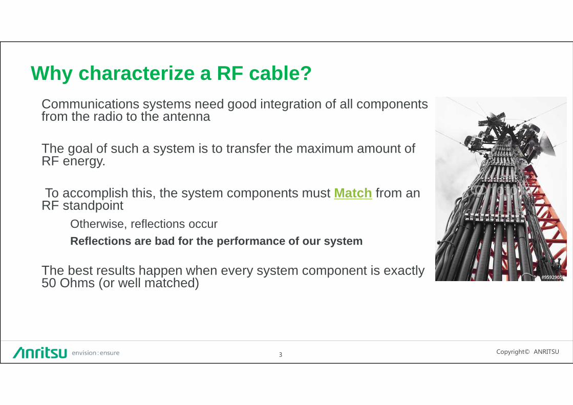
Why characterize a RF cable?Communications systems need good integration of all components from the radio to the antenna
The goal of such a system is to transfer the maximum amount of RF energy.
To accomplish this, the system components must Match from an RF standpoint
Otherwise, reflections occurReflections are bad for the performance of our syst em
The best results happen when every system component is exactly 50 Ohms (or well matched)

Copyright© ANRITSU4
The ideal world of transmission lines• Ideally a device has exactly it‘s characteristic impedance (e.g. 50 Ohm)
• Transmission Line• Transmitter
• Receiver
• Impedance matching enables maximum power transmission
Input Output
50 Ohm
50 Ohm
TransmissionLine
TransmitPower
ReceivedPower
≈
Maximum power transmission

Copyright© ANRITSU5
The real world of transmission lines• DUT (Device under Test) has an impedance different to the characteristic impedance
• Reflection coefficient r = V refl / Vtrans
• Transmission coefficient Pout / Pin
ReflectedPower P refl
Input Output
TransmissionLine Received
Power P out
TransmitPower P in
≈
Z ≠ 50 Ohm

Copyright© ANRITSU6
Coaxial cablesImpedance of coaxial transmission lines
• Relationship between inner- and outer diameter defines impedance of a coaxial cable
• Dielectric material
• Propagation velocity
Examples of coaxial cables used in communication systems
• Aircore dielectric
• Extremely low loss
• Coaxial cables
• Polyethylene solid
• Polyethylene foam
• Teflon (PTFE)
• Radiating cables
• Underground radio communication
• Impedance mostly 50 Ohm
• 75 Ohm for video cables and satellite IF cables
• 100 Ohm (Twisted Pair, Ethernet, symetrical transmission lines)
Inner diameter D ofouter conductor
Outer diameter d ofcenter conductor

Copyright© ANRITSU7
Why Z = 50 Ohms?
Good compromise

Copyright© ANRITSU8
Upper useable frequencyDominant propagation mode for electromagnetic waves in coaxial cable is TEM mode
Since a coaxial cable supports TEM, TE and TM electromagnetic wave propagation modes, the TE and TM modes will come into existent for sufficiently high operating frequency

Copyright© ANRITSU9
R e t u r n L o s s a n d V S W R

Copyright© ANRITSU10
The basic reflectometerReturn Loss measurement require a reflectometer
• Distinguish between transmitted and reflected waves
Generator
Vefl
DUTS11
Vtransmit
Directional Coupler,Bridge
≈
r = Vrefl / Vtransmit
Z ≠ Z0
Vrefl
Vtransmit
No reflectometer is ideal → Calibration necessary
Copyright© ANRITSU11
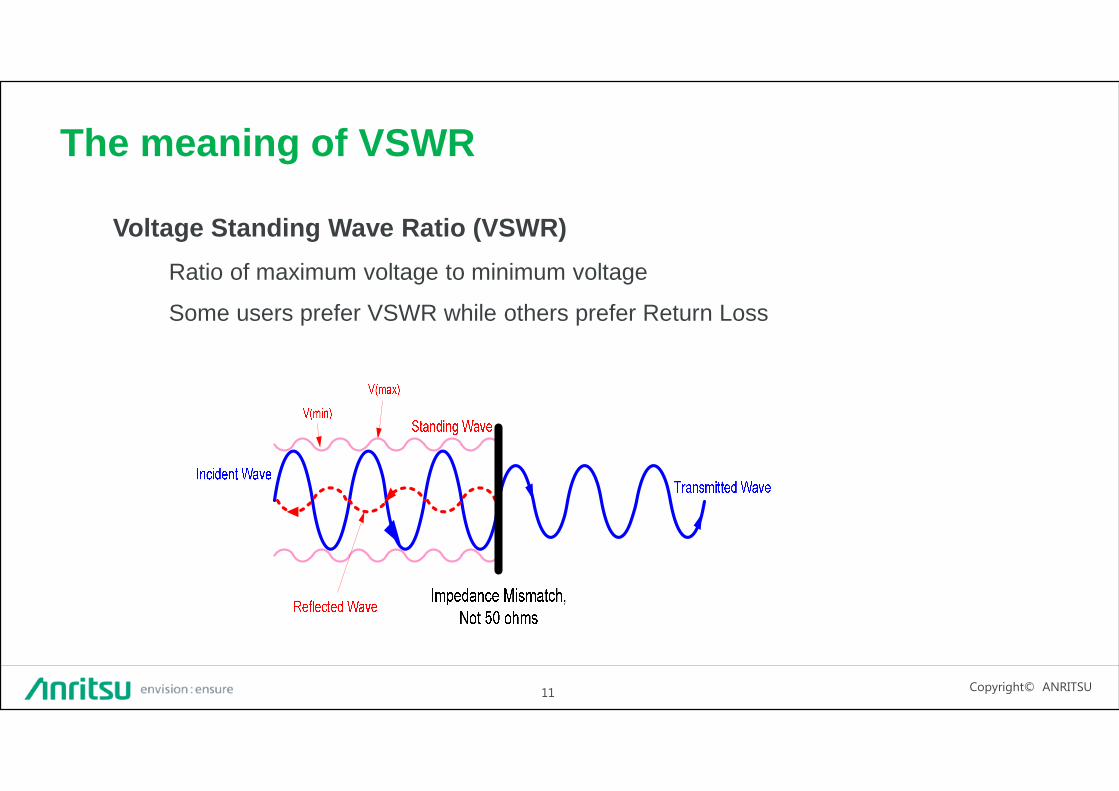
The meaning of VSWR
Voltage Standing Wave Ratio (VSWR)
Ratio of maximum voltage to minimum voltage
Some users prefer VSWR while others prefer Return Loss

Copyright© ANRITSU12
Return Loss or VSWR: What is better?
Reflection Coefficient: r = Vrefl / Vforward
r = (VSWR-1) / (VSWR+1)
Return Loss: RL[dB] = - 20 x log ( r )
(V)SWR (Voltage Standing Wave Ratio) VSWR = ( 1 + r ) / ( 1 - r )
Rho (linear reflection) ρ = Z - Z0 / Z + Z0
What do you prefer?Both gets the job done

Copyright© ANRITSU13
VSWR vs Return Loss
VSWR Return Loss (dB) Description 1.0:1 ∞ Perfect match. Cannot be done.
1.2:1 21 Very good match, very little reflection. (Often a design goal)
1.4:1 15 Acceptable match, acceptable amount of reflection.
3:1 6 Terrible match, significant reflections. Something is definitely wrong.
∞:1 0 Total Reflection. No signal is getting past the reflection point.
Comparison of VSWR and Return Loss

Copyright© ANRITSU14
Typical coaxial cable parameters
Copyright© ANRITSU15
Return Loss: Just connect the cable?
So you have bought a nice Anritsu VNA and now want to measure your cable...

Copyright© ANRITSU16
Return Loss: Just connect the cable?
Is this the correct Return Loss of a 50m cable?
Copyright© ANRITSU17
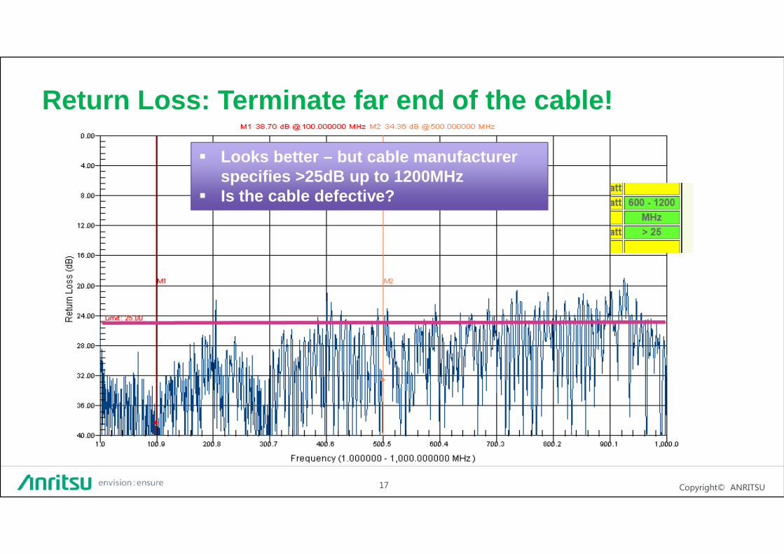
Return Loss: Terminate far end of the cable!
Looks better – but cable manufacturer specifies >25dB up to 1200MHz
Is the cable defective?

Copyright© ANRITSU18
Return Loss = Sum of all reflection vectors
+ +
=
Connector ConnectorCable
Complete Assembly

Copyright© ANRITSU19
Cable without connectors: Distance to Fault & Gatin g
Cable is in Spec! We have to remove influence of connectors to see
true behaviour of the cable Complicated measurement with Time Domain and Gating

Copyright© ANRITSU20
What‘s this noise on the RL measurement? No noise! True behavious of a long cable...
You even can calculate the lenght of the cable by the distance of the ripples

Copyright© ANRITSU21
Measured S11 as a function of frequency

Copyright© ANRITSU22
Smith Chart: Another way to display Impedances
M1: 3.50MHz, Z = 23.3 Ω – j2.6 Ω
M1: 3.50MHz, Z = 59.8 Ω – j85.7 Ω
Smith Chart is often used for Impedance Matching
Copyright© ANRITSU23
C a b l e L o s s
Slide Title or URL23
Copyright© ANRITSU24
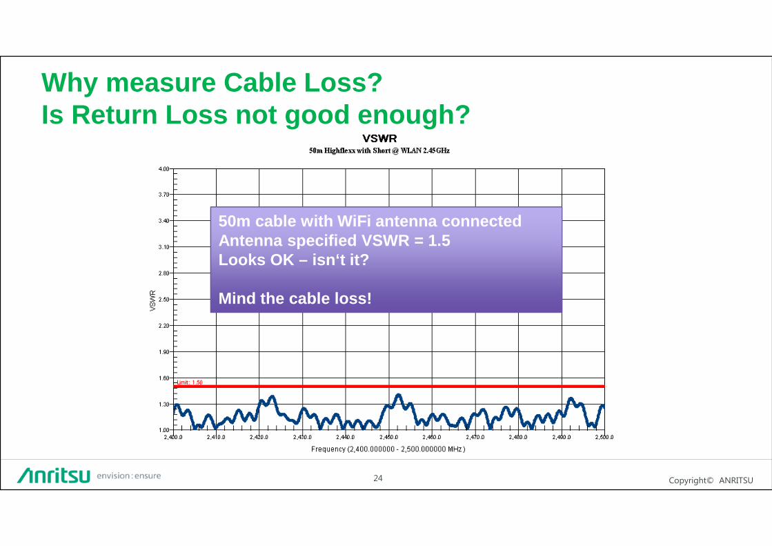
Why measure Cable Loss? Is Return Loss not good enough?
50m cable with WiFi antenna connectedAntenna specified VSWR = 1.5Looks OK – isn‘t it?
Mind the cable loss!
Copyright© ANRITSU25
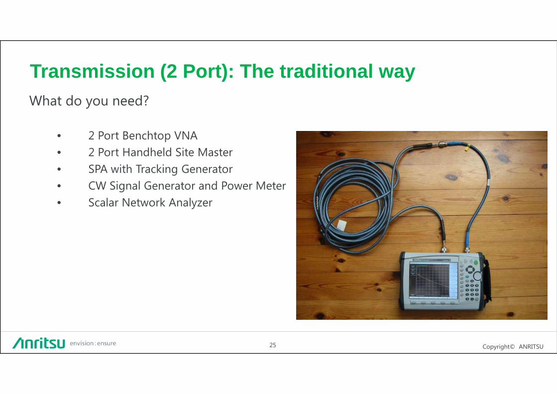
Transmission (2 Port): The traditional wayWhat do you need?
• 2 Port Benchtop VNA
• 2 Port Handheld Site Master
• SPA with Tracking Generator
• CW Signal Generator and Power Meter
• Scalar Network Analyzer

Copyright© ANRITSU26
Transmission (2 Port): The traditional wayWhat do you get?
• Normally excellent results for cable loss
• ... and Return Loss (1 Path 2 Port Cal)
Copyright© ANRITSU27
Transmission (2 Port): The problem!
Can‘t reach the far end of the cable• Cable already installed in a building, vehicle, aircraft,
tower, ship, etc.
What to do?• Buy a looooooong testport cable?
• Use another measurement methode?

Copyright© ANRITSU28
Method I - 1 Port Cable LossMain application: Insertion Loss of low loss cables in antenna systems
• Calculation based on Return Loss measurement
• Divides Return Loss value by factor 2
• Far end of cable must be terminated with Short (or Open)
Urefl
Short
S11Uhin
Directional Coupler,Bridge
Generator
≈ Cable
Insertion Loss
Insertion Loss
S11 = RL = 2 x Insertion Loss

Copyright© ANRITSU29
1 Port Cable Loss vs. 2 Port Transmission
1 Port Cable Loss: Mainly used for low loss feeder cables from BTS to Antenna

Copyright© ANRITSU30
1 Port Cable Loss
Works best with low loss cables
• If return loss values (with short) become similar to terminated return loss than „noise“ is superimposed to cable loss measurements
Cable terminated with load
Cable terminated with short

Copyright© ANRITSU31
Method II: External Transmission Sensor
Like in the good old days of Scalar Analyzers...

Copyright© ANRITSU32
Method II: External Transmission SensorComparable results to a traditional 2 Port measurements

Copyright© ANRITSU33
T i m e D o m a i n
Slide Title or URL33

Copyright© ANRITSU34
Time DomainAdditional measurement to VSWR/Return Loss
• Can‘t replace a Return Loss measurement!
Information where the reflection happens
Different names are often used:
• Time Domain• TDR Measurement• Distance to Fault (DTF)• FFT Measurement• FDR
Time/Lenght
Am
plitu
de (
dB)
0dB = total reflection
-30dB = input connector

Copyright© ANRITSU35
Limitations of VSWR/RL measurementVSWR/RL measurement does not show the location of reflexions
Connector tight Connector loose
Example: 2 x 6m cable with connector in the center
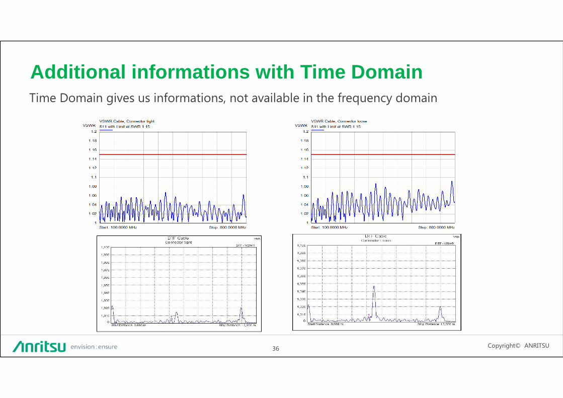
Copyright© ANRITSU36
Additional informations with Time DomainTime Domain gives us informations, not available in the frequency domain

Copyright© ANRITSU37
TDR versus FDRAnritsu VNAs are using FDR technique (Frequency Domain Reflectometry)
Frequency
SourceSpectralDensity
f1 f2
FDR
TDR
Less than 2% of the TDR pulse power is in the operation frequency range
Copyright© ANRITSU38
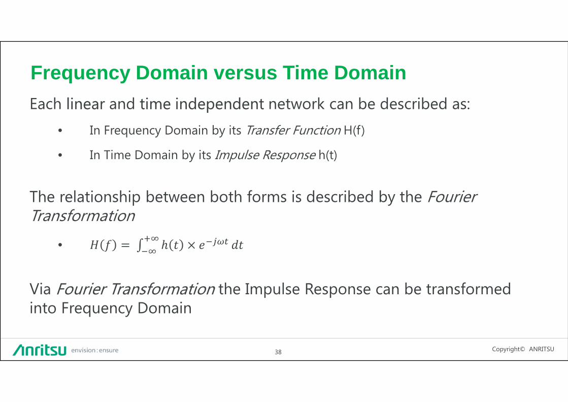
Frequency Domain versus Time Domain
Each linear and time independent network can be described as:
• In Frequency Domain by its Transfer Function H(f)
• In Time Domain by its Impulse Response h(t)
The relationship between both forms is described by the Fourier Transformation
• = ℎ ×
Via Fourier Transformation the Impulse Response can be transformed into Frequency Domain
Copyright© ANRITSU39
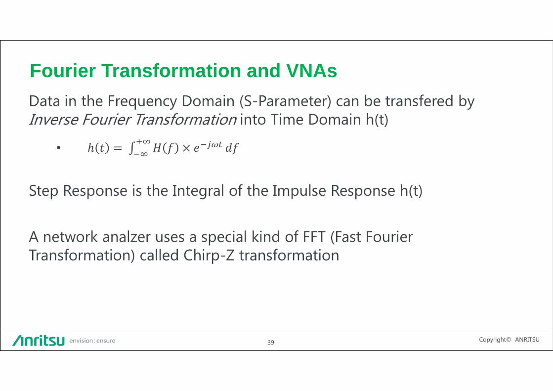
Fourier Transformation and VNAs
Data in the Frequency Domain (S-Parameter) can be transfered by Inverse Fourier Transformation into Time Domain h(t)
• ℎ = ×
Step Response is the Integral of the Impulse Response h(t)
A network analzer uses a special kind of FFT (Fast Fourier Transformation) called Chirp-Z transformation

Copyright© ANRITSU40
Time Domain: The data flow
RL / VSWR DataFrequency
Domain
WindowFunction
Inverse Fourier-transformation
( IFT )
Data inTime Domain
f1 f2
VS
WR
Time Domain
= Frequency Domain
Copyright© ANRITSU41
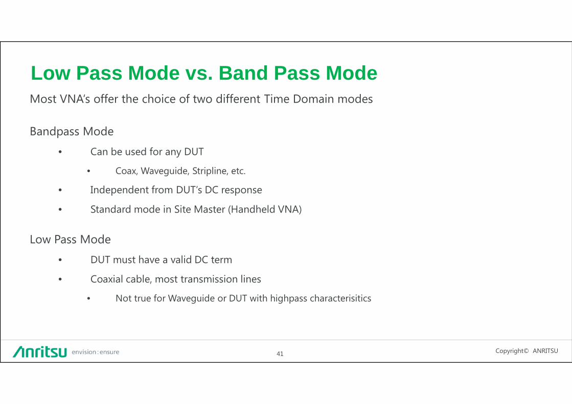
Low Pass Mode vs. Band Pass ModeMost VNA‘s offer the choice of two different Time Domain modes
Bandpass Mode
• Can be used for any DUT
• Coax, Waveguide, Stripline, etc.
• Independent from DUT‘s DC response
• Standard mode in Site Master (Handheld VNA)
Low Pass Mode
• DUT must have a valid DC term
• Coaxial cable, most transmission lines
• Not true for Waveguide or DUT with highpass characterisitics
Copyright© ANRITSU42
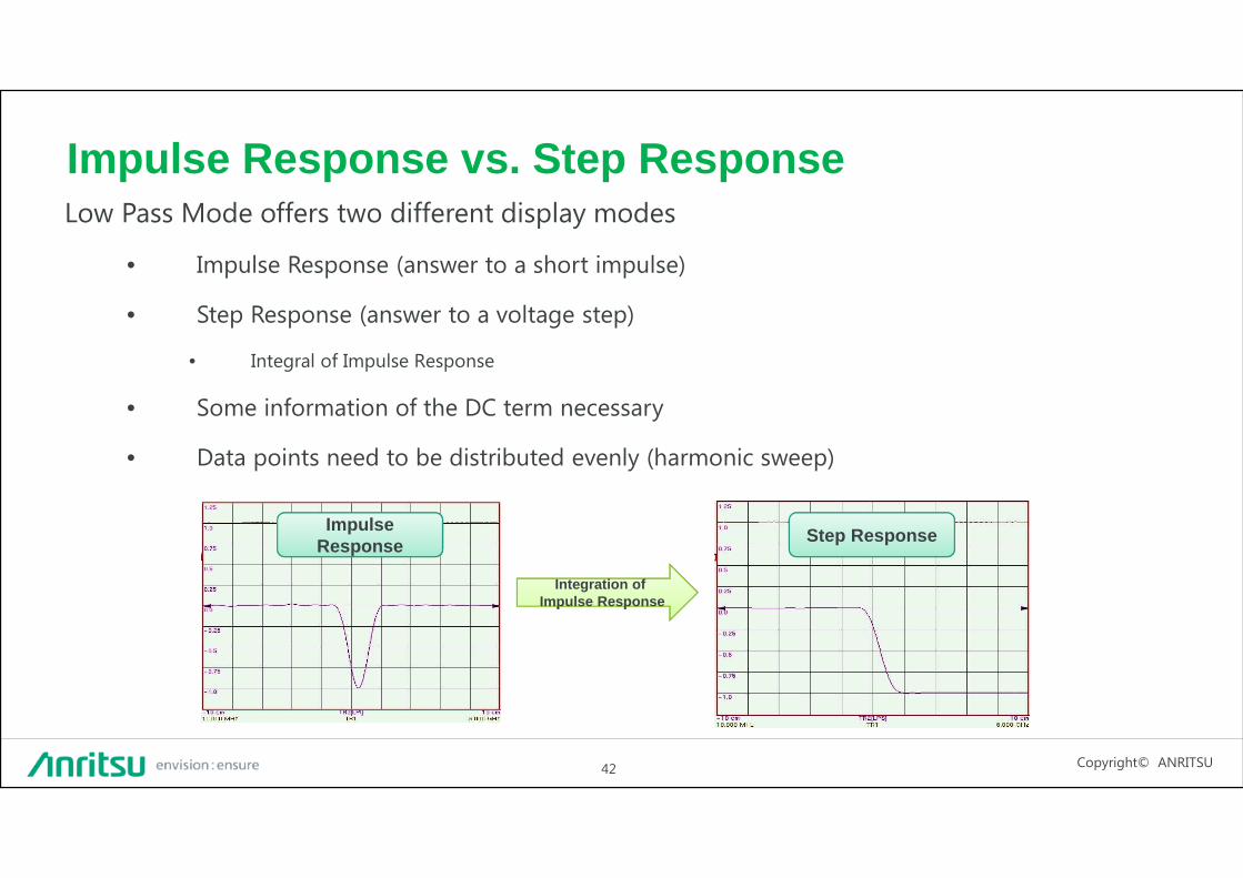
Impulse Response vs. Step ResponseLow Pass Mode offers two different display modes
• Impulse Response (answer to a short impulse)
• Step Response (answer to a voltage step)
• Integral of Impulse Response
• Some information of the DC term necessary
• Data points need to be distributed evenly (harmonic sweep)
Integration ofImpulse Response
Integration ofImpulse Response
Impulse Response Step Response
Copyright© ANRITSU43
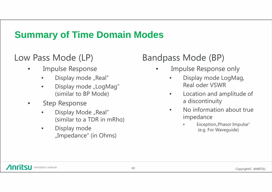
Low Pass Mode (LP)• Impulse Response
• Display mode „Real“
• Display mode „LogMag“ (similar to BP Mode)
• Step Response
• Display Mode „Real“ (similar to a TDR in mRho)
• Display mode „Impedance“ (in Ohms)
Bandpass Mode (BP)• Impulse Response only
• Display mode LogMag, Real oder VSWR
• Location and amplitude of a discontinuity
• No information about true impedance• Exception„Phasor Impulse“
(e.g. For Waveguide)
Summary of Time Domain Modes

Copyright© ANRITSU44
Beatty Standard (Stepped Airline)
25Ω50Ω 50Ω
• Often used as example to demonstrate time domain functionality
Copyright© ANRITSU45
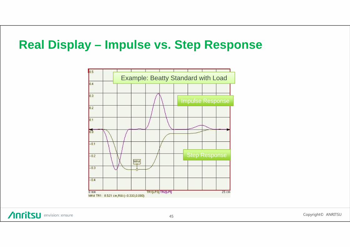
Real Display – Impulse vs. Step Response
Example: Beatty Standard with Load
Impulse Response
Step Response

Copyright© ANRITSU46
Real Display vs. LOG Display – Impulse Response
Impulse Response LOG MAG
Example: Beatty Standard with Load

Copyright© ANRITSU47
Impedance display – Step Response
Step Response withdirect Impedance reading
Example: Beatty Standard with Load

Copyright© ANRITSU48
Time Domain: Practical hints for coax cables
Important parameters for fault location on cables
• Cable parameter• Propagation Velocity: Vrel• Loss: dB/m
• Frequency range
• Windowing

Copyright© ANRITSU49
DTF: Just connect the cable?Perform a Full Reflection Calibration
(OSL)
Switch to DTF Return Loss/Time Domain
Connect the cable....
Is this my cable?Looks weird?
Distance (0.00 – 60.0m)
DT
F-R
L (d
B)
Copyright© ANRITSU50
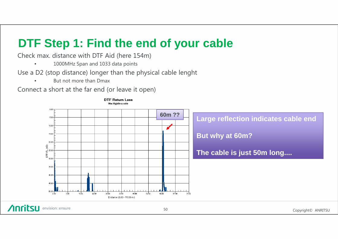
DTF Step 1: Find the end of your cableCheck max. distance with DTF Aid (here 154m)
• 1000MHz Span and 1033 data points
Use a D2 (stop distance) longer than the physical cable lenght• But not more than Dmax
Connect a short at the far end (or leave it open)
Large reflection indicates cable end
But why at 60m?
The cable is just 50m long....
60m ??
Copyright© ANRITSU51
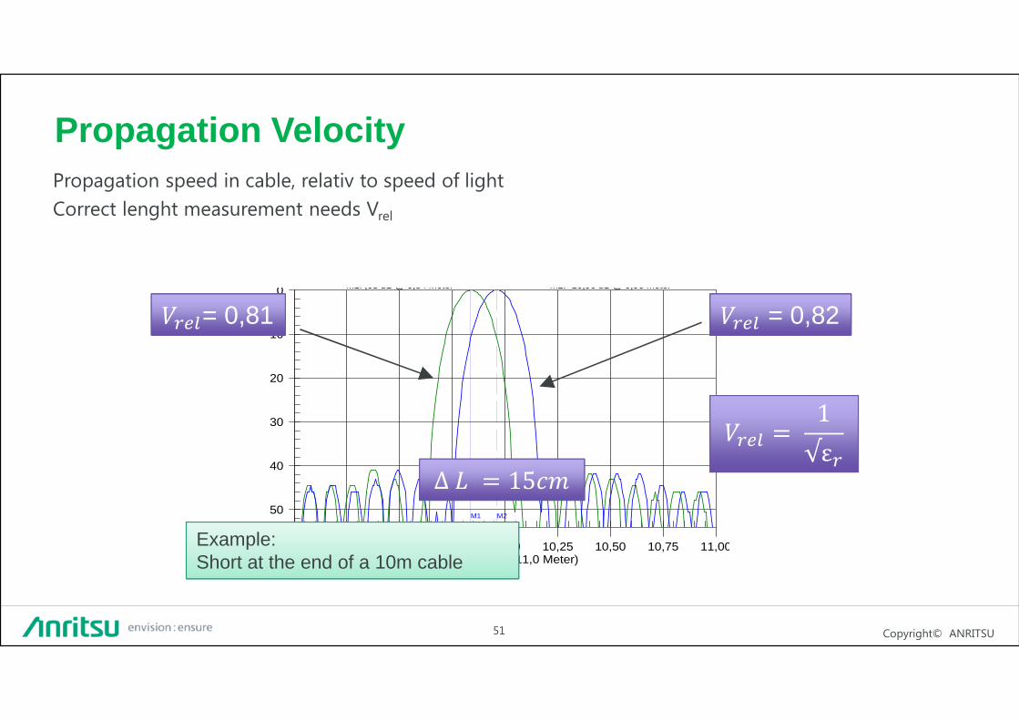
Propagation VelocityPropagation speed in cable, relativ to speed of light
Correct lenght measurement needs Vrel
-50
-40
-30
-20
-10
0
9,00 9,25 9,50 9,75 10,00 10,25 10,50 10,75 11,00
Vergleich
DTF ZOOM 3
M1 M2
Distance (9,0 - 11,0 Meter)
M1: ,03 dB @ 9,84 Meter M2: -10,96 dB @ 9,96 Meter
= 0,81 = 0,82
∆ = 15∆ = 15Example:Short at the end of a 10m cable
= 1√ε = 1√ε

Copyright© ANRITSU52
DTF Step 2: Set the Prop VelocityInstrument sets propagation velocity to 1 (air)
• Propagation in cable is always slower than speed of light
• Use cable from cable list
• Enter Prop. Velocity manually (here 0.83)
Cable end now @ 50m
But why is amplitude at 13dB (short = 0dB)?
-13dB ??
Copyright© ANRITSU53
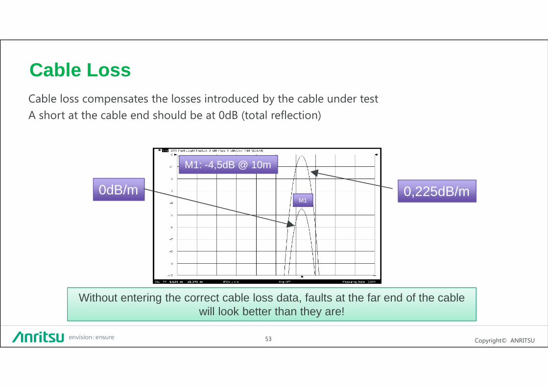
Cable LossCable loss compensates the losses introduced by the cable under test
A short at the cable end should be at 0dB (total reflection)
0dB/m 0,225dB/m
Without entering the correct cable loss data, faults at the far end of the cable will look better than they are!
M1: -4,5dB @ 10m
M1

Copyright© ANRITSU54
DTF Step 3: Set the Cable LossInstrument sets cable loss to 0dB/m
• Cable attenuation needs to be taken into account
• Use cable from cable list
• Enter cable loss manually (here 0.13dB/m)
Cable end @ 50m
Short @ 0dB
0dB @ 50m !!!
Copyright© ANRITSU55
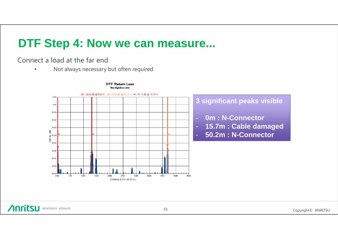
DTF Step 4: Now we can measure...Connect a load at the far end
• Not always necessary but often required
3 significant peaks visible
- 0m : N-Connector- 15.7m : Cable damaged- 50.2m : N-Connector
Copyright© ANRITSU56
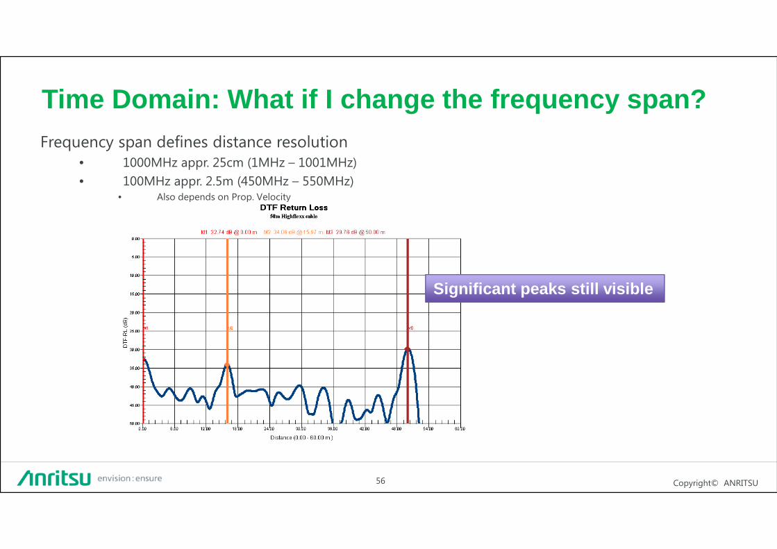
Time Domain: What if I change the frequency span?Frequency span defines distance resolution
• 1000MHz appr. 25cm (1MHz – 1001MHz)
• 100MHz appr. 2.5m (450MHz – 550MHz)• Also depends on Prop. Velocity
Significant peaks still visible

Copyright© ANRITSU57
Frequency range determines distance resolution
!"#$%&#'()"'% ≈ 1
+$%,"!"#$%&#'()"'% ≈
1
+$%,"
6GHz Span
1,5GHz Span
3GHz Span
Example: Beatty Standard with Load
Frequency Domain
Time Domain

Copyright© ANRITSU58
Distance Resolution
-#'()"'% ≈ 150
/&012$%34-#'()"'% ≈ 150/&012$%34
-')%5&"2 -("'% -#'()"'% = 0,577∆/-')%5&"2 -("'% -#'()"'% = 0,577∆/
= 37109∆/ = /: ;< − /: >
= 37109 m/s∆/ = /: ;< − /: > [Hz]
z.B. Span = 6GHz → 25mm Resolution (LP Mode, Air)
Copyright© ANRITSU59
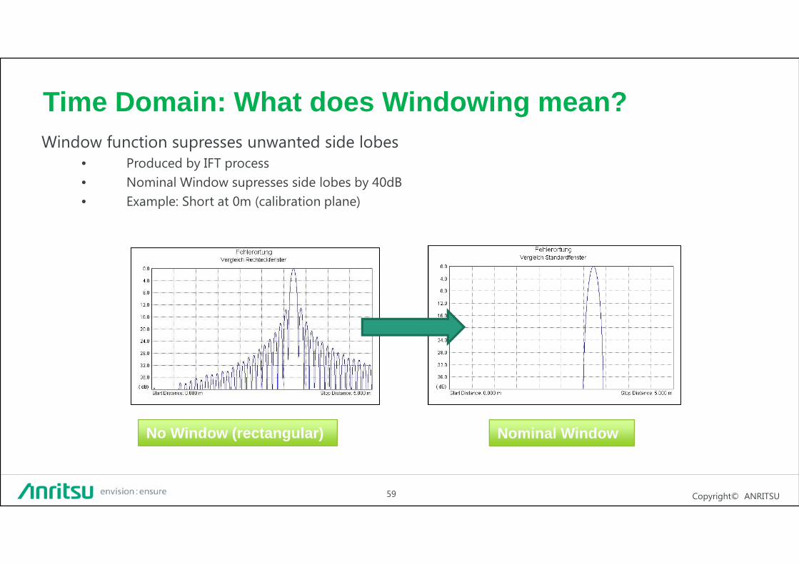
Time Domain: What does Windowing mean?Window function supresses unwanted side lobes
• Produced by IFT process
• Nominal Window supresses side lobes by 40dB
• Example: Short at 0m (calibration plane)
No Window (rectangular) Nominal Window

Copyright© ANRITSU60
Which Window Function to choose?Compromise between distance resolution and sidelobe supression
• Typical Window functions in a VNA
Rectangular Window
Nominal Sidelobe
Low Sidelobe

Copyright© ANRITSU61
Which Window Function to choose?Side Lobes with rectangular window could be seen as discontinuities......
Rectangular Window
Nominal Sidelobe
Example: Beatty Standard withLoad
Nominal Window is best compromise

Copyright© ANRITSU62
Data PointsNumber of data points does not have influence of distance resolution!
200 Data Points2000 Data Points
Example: 20dB Offset Load at end of 10m cable
∆F = 2000MHz