Public Access CopyDO NOT REMOVEfrom room 208.

STATE OF DELAWAREUNIVERSITY OF DELAWARE

DELAWARE GEOLOGICAL SURVEY

Robert R. Jordan, State Geologist

BULLETIN No. 14

HYDROLOGY OF THE COLUMBIA (PLEISTOCENE) DEPOSITSOF DELA~~ARE: AN APPRAISAL OF AREGIONAL

WATER-TABLE AQUIFER

BY

RICHARD Ht JOHNSTONHYDROLOGIST, U. S. GEOLOGICAL SURVEY

NEWARK, DELAWARE

JUNE, 1973

STATE OF DELAWAREUNIVERSITY OF DELAWARE

DELAWARE GEOLOGICAL SURVEY

Robert R. Jordan, State Geologist

BULLETIN No. 14

HYDROLOGY OF THE COLUMBIA (PLEISTOCENE) DEPOSITSOF DELAWARE: AN APPRAISAL OF AREGIONAL

WATER-TABLE AQUIFER

BY

RICHARD H. JOHNSTONHYDROLOGIST, U. S. GEOLOGICAL SURVEY

PREPARED BY THE UNITED STATES GEOLOGICAL SURVEYIN COOPERATION WITH THE

DELAWARE GEOLOGICAL SURVEY

NEWARK, DELAWARE

JUNE, 1973

CONTENTS

Page

vi

1124

55

• 812

12• 16• 21• 24

• 27

• ~1

• 34• 35

4046

• 484849

• 52

• 52• 56

• 63

65

• 75

•

••

•

•

•

•

•

•••

•

••

•

•

•• • •

. .....of the Investigation

HYDROGEOLOGY OF THE COLUMBIA (PLEISTOCENE) DEPOSITS.Lithologic Character and Stratigraphy.Areal Extent and Saturated Thickness •Hydraulic Characteristics. • • • •

Transmissivity and Storage CoefficientDetermined by Aqui.fer Tests.. ••••

Houston .aquifer test. • •• ••••Middletown aquifer test • •• •Milton aquifer test • • •• ••••

Aquifer Coefficients Estimated by ReconnaissanceMethods.. •• •• ••

Areal Distribution of Transmissivity andHydraulic Conductivity.. •••

GROUND-WATER HYDROLOGY • • • • • • • • • •Changes in Storage (Water-Level Fluctuations). •Ground-Water Discharge. • •Ground-Water Recharge • ••• •

GROUND-WATER DEVELOPMENT.. • •Yield and Specific Capacity of Wells. • • • •Current withdrawals. •Potential Development. • • • • • • •

General Availability of Water from theColumbia Deposits • •• ••

Availability of Large Ground-Water Supplies. •

QUALITY OF WATER AND GROUND-WATER CONTAMINATION. •

APPLICATION OF FINDINGS • ••• •••

REFERENCES •• •

ABSTRACT. • •

INTRODUCTION.Scope and PurposeAcknowledgments •Previous Work.

iii

ILLUSTRATIONS

Figure 1. Locations of wells and stream-gagingstations referred to in the text

2. Structure contour map of the base ofthe Columbia ,(Pleistocene) deposits

3. Saturated thickness map of theColumbia (Pleistocene) deposits inDelaware • • • • •

4. Section through Houston aquifer-testsite showing lithology, wellconstruction, and well spacing •

5. Logarithmic plot of drawdown againsttime for~id-aquifer observationwell (Md24-l) at Houston aquifertest, May 17-19, 1971 •

6. Logarithmic plot of drawdown againsttime for observation well Md24-2(near base of aquifer) at Houstonaquifer test, May 17-19, 1971

7. Logarithmic plot of drawdown againsttime for observation well Fb34-l7(base of aquifer) at Middletownaquifer test, May 7-8, 1970. •

8. Logarithmic plot of drawdown againsttime for mid-aquifer observationwell (Ng55-3) at Milton aquifertest, Dec. 8-10, 1970 •

9. Transmissivity map of the Columbia(Pleistocene) deposits in Delaware.

10. Hydrograph of water level in shallowobservation well, Md22-l, andprecipitation at Milford, Del.,1962-1971 •

11. Hydrographs of water levels in fourobservation wells tapping theColumbia deposits under differenthydrogeologic conditions •

12. Ground-water runoff and overlandrunoff at Stockley Branch, ascompared to ground-water levels,May - Sept., 1971

13. Specific-capacity frequency graph forlarge-diameter wells tapping theColumbia deposits

14. Drawdown around a hypothetical pumpedwell discharging at 500 gallons perminute from Columbia deposits ofaverage transmissivity. .

iv

•

Page

3

9

11

17

18

20

23

26

32

36

38

42

50

53

Figure 15. Hydrologic conditions in part ofBeaverdam Creek basin nearMilton, Del••

TABLES

Page

59

Table 1. Correlation chart showing stratigraphicnomenclature used for the Pleistocenedeposits of Delaware and adjacentMaryland

2. Summary of aquifer tests of theColumbia deposits in Delaware

3. Aquifer coefficients estimated byreconnaissance methods.

4. Streamflow and ground-water runofffrom six basins in central andsouthern Delaware

5. Estimated pumpage of water from tneColumbia deposits in Delawareduring 1970. • • •

6. Chemical constituents in water from19 wells tapping the Columbiadeposits

7. Yield and specific capacity oflarge-diameter wells tapping theColumbia (Pleistocene) deposits andestimated transmissivity of theaquifer. •

v

6

14

30

44

51

64

68

HYDROLOGY OF THE COLUMBIA (PLEISTOCENE) DEPOSITS

OF DELAWARE: AN APPRAISAL OF A REGIONAL

WATER-TABLE AQUIFER

by

Richard H. Johnston

ABSTRACT

The Columbia (Pleistocene) deposits of Delaware form aregional water-table aquifer, which supplies about half theground water pumped in the State.

The aquifer is composed principally of sands which occuras channel fillings in northern Delaware and as a broad sheetacross central and southern Delaware. The saturated thick­ness of the aquifer ranges from a few feet in many parts ofnorthern Delaware to more than 180 feet in southern Delaware.Throughout 1,500 square miles of central and southernDelaware (75 percent of the State's area), the saturatedthickness ranges from 25 to 180 feet and the Columbiadeposits compose all or nearly all of the water-table aquifer.

The transmissivity of the aquifer varies greatly reflec­ting local changes in lithology (from fine sand to coarsesand and gravel) and changes in saturated thickness. However,the hydraulic data indicate that the Columbia depositseffectively act as a medium to coarse sand aquifer. Theaverage transmissivity in central and southern Delaware isabout 7,000 ft 2/day (53,000 gpd/ft), and the average hydraulicconductivity is about 90 ft/day. Six areas of above-averagetransmissivity have been identified in central and southernDelaware, where transmissivity ranges from 10,000 ft 2/day

(75,000 gpd/ft) to 22,000 ft 2/day (170,000 gpd/ft). Thesehigh transmissivity tracts correspond to "troughs" in astructure contour map on the base of the Columbia deposits,as well as sites of above-average saturated thickness. Thehighest transmissivity values occur where the saturatedsection contains primarily "clean" coarse sand and inter­bedded gravel and not necessarily where the saturatedsections are thickest.

The small Coastal Plain streams of central and southernDelaware are incised into the upper part of the Columbia

vi

deposits and derive about three-quarters of their flow fromground-water discharge. Much of the time, the streams simplyact as shallow drains from the aquifer. Separation ofstreamflow hydrographs indicate that the average ground-waterrunoff from the Columbia deposits is about 800 mgd (milliongallons per day). The average rate of recharge to theaquifer (computed from ground-water runoff values during thenongrowing season) is approximately 1 billion gallons per day(equivalent to 13-14 inches annually).

Present pumpage (33 mgd) is small compared to thenatural discharge from the aquifer. The aquifer is capableof yielding a much greater quantity of water~ however, largewithdrawals will be accompanied by corresponding decreases instreamflow (unless tha pumped water is returned to thestreams or the aquifer).

The specific capacity of large-diameter wells rangesfrom about 5 to 100 gpm/ft (gallons per minute per foot ofdrawdown) and averages 28 gpm/ft. Throughout most of centraland southern Delaware, it is possible to construct large­diameter wells capable of producing 500 gpm or more for shortperiods of time. However, the best method of obtainingdependable water supplies in excess of 1 mgd is to locatewells in areas of high transmissivity adjacent to streamscharacterized by high base flow. Such wells may obtain largeamounts of water by diverting the natural discharge from theaquifer to the stream as well as by diverting water alreadyin the stream through the streambed into the aquifer.

Water from the Columbia deposits is generally soft,slightly acidic, and characterized by low dissolved-solidcontent. High iron content and low pH are the only naturalcharacteristics that may require treatment. However, theposition of the Columbia deposits near land surface makes theground water particularly susceptible to contamination.Instances of contamination reported to date have resultedfrom salt-water intrusion in a few coastal areas, effluentfrom septic tanks, leachates from landfills, and accidentalspills.

vii

INTRODUCTION

Scope and Purpose of the Investigation

The Columbia deposits of Delaware form a regionalwater-table aquifer which is the State's most importantground-water resource. The aquifer supplies about half thecurrent ground-water pumpage in the State and is capable ofsupplying a much greater amount of water.

The purpose of the investigation described in thisreport was to make a quantitative hydrologic appraisal ofthe Columbia (Pleistocene) deposits in Delaware. Specif­ically, it was hoped to better define the hydrauliccharacteristics of this regional water-table aquifer, toestimate recharge to and discharge from tr~ aquifer, and toascertain the long-term availability of water from theaquifer. The lithologic character and thickness of theColumbia deposits were reasonably well known from previousstudies~ however, the aquifer coefficients (transmissivityand storage coefficients) were known at only a few isolatedaquifer test sites. A major aim of the study was to obtainadditional values of aquifer coefficients by reconnaissancetechniques and to compare them with values obtained at afew selected aquifer test sites.

Early in the study it became evident that the relationof ground water to surface water would have to be investi­gated. It was determined that the streams in central andsouthern Delaware obtained most of their flow from ground­water discharge (considered equivalent to base flow) ratherthan from overland runoff. Much of the time the streamssimply acted as drains from the aquifer~ therefore,estimates of long-term discharge from the aquifer could bedetermined from base-flow data. Furthermore, a closecorrelation was established between ground-water levels andbase flow in several small basins. Lowering of ground­water levels by pumping water from the aquifer wouldundoubtedly reduce streamflow. Thus, any statement as tothe long-term availability of ground water must considerthe effect on streamflow. It was decided to study therelation of ground water to surface water in several smallbasins and apply the results of these studies to a state­wide appraisal of the shallow aquifer-stream system. Thestudies of small basins are summarized in a short paper(Johnston, 1971) and will be described in detail in anotherpaper, as yet unpublished.

The transmissivity of the Columbia deposits and,therefore, the yield and specific capacity of wells was

1

known to vary widely throughout the Delaware Coastal Plain.The preparation of a statewide transmissivity map was givenhigh priority during this study. In preparing such a map,it was hoped to make use of reconnaissance techniques(utilizing base-flow recession and ground-water-levelrecessions) to estimate transmissivity. If the attemptwere successful, these techniques could also be useful infuture prospecting for large ground-water supplies inDelaware.

The area investigated included all the Coastal Plainof Delaware. However, particular emphasis was placed oncentral and southern Delaware, where the Columbia depositsform a regional water-table aquifer. This area of emphasisincludes all of Sussex County and most of Kent County(Figure 1). The locations of counties and major towns inDelaware, as well as streams, gaging stations, observationwells, production wells, and aquifer test sites referred toin the text are shown in Figure 1.

Acknowledgments

-The writer wishes to express his appreciation toRobert R. Jordan, State Geologist and cooperator in thisstudy, for providing much assistance, especially during thefield phases of the investigation. Kenneth D. Woodruff andJohn C. Miller, hydrogeologists with the Delaware GeologicalSurvey, assisted during pumping tests, and Mr. Woodruffgeophysically logged several test holes. In addition,exploratory holes were drilled and piezometer tubes wereinstalled using a University of Delaware combination augerand rotary drill rig operated by Boris J. Bilas of theDelaware Geological Survey.

Many individuals aided the writer during the study.It is not possible to single out everyone by name 1 however,special thanks are given to Mr. and Mrs. James B. Carpenter,who permitted construction of wells on their property foran aquifer test. Thanks are also given to Paul E. White andSons, Inc. and Delmarva Drilling Company for providing manywell logs and pumping-test data.

The writer also wishes to thank his colleagues in theU. S. Geological Survey 1 Philip Pfannebecker, R. H. Simmons,E. M. Cushing, K. R. Taylor, and I. H. Kantrowitz forsuggestions made during the study and for supplying unpub­lished basic data.

The investigation and report preparation were under thedirection of W. F. White, District Chief, U. S. GeologicalSurvey.

2

O"d22~1

OBSERVATION WELL

o 4 ISMILESf .. !

EXPLANA TlON

.4870

STREAM-GAGING STATION

a1lldM-1 TO.

WELL WITH AQUIFER TEST DATA LISTED IN TABLE It

.LdS3-1

MODERATE TO LARGE CAPACITY WELL;CONSTFEATURES. YIELD. AND SPECIFICCAPACITY LISTED INTABLE 7.

!rIO'

18'lS'

!rIO'

11'00' 0 1I~

\II 0

\'<-??~

~...

lI'4S'

1t'.I'

FIGURE I. LOCATIONS OF WELLS AND STREAM-GAGING STAnONS REFERRED TO IN THETEXT.

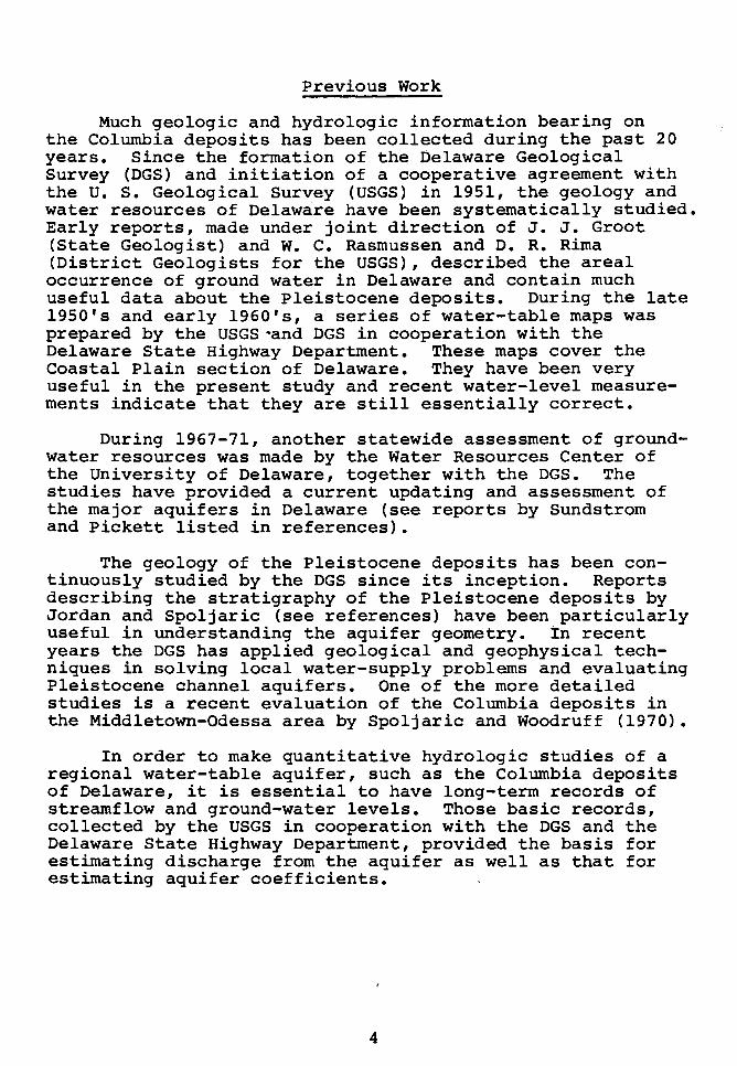
Previous Work

Much geologic and hydrologic information bearing onthe Columbia deposits has been collected during the past 20years. Since the formation of the Delaware GeologicalSurvey (DGS) and initiation of a cooperative agreement withthe U. S. Geological Survey (USGS) in 1951, the geology andwater resources of Delaware have been systematically studied.Early reports, made under joint direction of J. J. Groot(State Geologist) and W. C. Rasmussen and D. R. Rima(District Geologists for the USGS), described the arealoccurrence of ground water in Delaware and contain muchuseful data about the Pleistocene deposits. During the late1950's and early 1960's, a series of water-table maps wasprepared by the USGS·and DGS in cooperation with theDelaware State Highway Department. These maps cover theCoastal Plain section of Delaware. They have been veryuseful in the present study and recent water-level measure­ments indicate that they are still essentially correct.

During 1967-71, another statewide assessment of ground­water resources was made by the Water Resources Center ofthe University of Delaware, together with the DGS. Thestudies have provided a current updating and assessment ofthe major aquifers in Delaware (see reports by Sundstromand Pickett listed in references).

The geology of the Pleistocene deposits has been con­tinuously studied by the DGS since its inception. Reportsdescribing the stratigraphy of the Pleistocene deposits byJordan and Spoljaric (see references) have been particularlyuseful in understanding the aquifer geometry. In recentyears the DGS has applied geological and geophysical tech­niques in solving local water-supply problems and evaluatingPleistocene channel aquifers. One of the more detailedstudies is a recent evaluation of the Columbia deposits inthe Middletown-Odessa area by Spoljaric and Woodruff (1970).

In order to make quantitative hydrologic studies of aregional water-table aquifer, such as the Columbia depositsof Delaware, it is essential to have long-term records ofstreamflow and ground-water levels. Those basic records,collected by the USGS in cooperation with the DGS and theDelaware State Highway Department, provided the basis forestimating discharge from the aquifer as well as that forestimating aquifer coefficients.

4

HYDROGEOLOGY OF THE COLUMBIA (PLEISTOCENE) DEPOSITS

Lithologic Character and Stratigraphy

Surficial sands of presumed Pleistocene age mantle theolder (Cretaceous and Tertiary) sediments nearly everywherein the Coastal Plain of Delaware. These sands form an uncon­fined aquifer of regional extent throughout the DelmarvaPeninsula. Because of their large areal extent and becauseseveral environments of deposition are represented, authorshave designated the Pleistocene deposits by several names.Some of the more recent nomenclature is listed in Table 1.

However, for the purpose of this report, a detailedstratigraphic nomenclature is not needed. The general term,"Columbia deposits," is used here and refers to all surficialsand and associated gravel, clay, and silt beds of presumedPleistocene age in Delaware. The term Columbia deposits, asused in this report, is synonymous with such terms asPleistocene deposits or Pleistocene aquifer. Use of theterm "Columbia" follows Jordan (1962), who proposed the nameColumbia Formation for the fluvial Pleistocene deposits ofnorthern and central Delaware and, where the deposits aresubdivisible into two formations in southern Delaware, thename Columbia Group (Table 1). A discussion of the histor­ical precedence for use of the term Columbia is given byJordan (1962). All recent reports of the Delaware Geolog­ical Survey have used the terms Columbia Group or Formationas have several recent reports of the Maryland GeologicalSurvey and the USGS (see for example: Back, 1966; Hansen,1966; and Otten, 1970). However, some objection has beenraised to use of the term "Columbia" for all the Pleistocenesediments in Delaware. Based on a recent geologic mapping,J. P. Owens of the USGS (oral communication, Oct. 1972,Table 1) believes that the Pleistocene deposits of northernand southern Delaware are too dissimilar in lithology andgenesis for use of one inclusive stratigraphic term such asColumbia Group.

The orange to reddish-brown sand beds which Rasmussenand others (1960) termed the Brandywine Formation ofPliocene (?) age and Hansen (1966) called the red gravellyfacies of the Salisbury Formation (Pleistocene), are con­sidered to be part of the Columbia (Pleistocene) depositsin this report. As noted by Jordan (1962), there is nodefinitive evidence for the age of these 'beds and recentgeologists have considered the unit as part of thePleistocene deposits. In general, the stratigraphic nameslisted in Table 1 are not used throughout this report. Anexception is the Beaverdam Sand - a readily identifiablewhite, medium sand found throughout southern Delaware.

5

en

RASMUSSEN AND JORDAN (1962) HANSEN (1966) OWENS (ORAL THIS REPORTOTHERS (1960) COM MUNICATION,

SUSSEX CO., DELAWARE DELAWARE SALISBURY, MD. AREAOCTOBER, 1972 )

DELAWARE

SERIES FORMATION SERIES FORMATION OR GROUP SERIES FORMATION OR 'FACIES' SERIESFORMATION OR 'FACIES' SERIES AOUIFER

N. DELAWARE S.DELAWARE N.DELAWARE S.DELAWARE

PARSONBURGSAND z 0::0 WALSTON ILl

~CLAY ti3 ~ -(I)ct

PAMLICO ~ :e0:: 1U

FORMATION 0:: ctcte:>0 ZCD ct (I)Z IL

0 ZIIL ~

.... 0- 0:: PARSONBURG=>~ (I)

ILl WALSTON IU ct => ct eX 0Z

SILTZ

~0 2 SAND Z ...J 0-

ILl IU 0:: 0 0 CD ILl0 0 0:: (!) ..... - 00 0 0 0- ~ .....~

u, ct~ Z ILl => ILl ct ILl IU(J) (I) CD 0 Z 0 Z ~ Z Z- ctILl IU 2 ~ 1U0::

(J) ILl 0:: IU IU...J ...J CD => ct o (!)

IU 0 0 0 0a. a. ~ ...J ~ 0 0 0 u, 0 0

=> 0 0:: ~ct Z ct .... Z ~ ~

...J (I) - 0 u, (J) Z 0 (I) (I)BEAVERDAM 0 e _CD IU0 ILl 2 ti :E ILl ~ ~ IU ILl

SAND 02 ...J=> ct ...J => ct ...J ...J

ct 0- ...J ~ 0 0- ct 2 0- 0-0 --0 0:: 0:: (I) 0::

0:: 0 0 ILl Z 0 ct-- u,IU~ IU u,

> CDct >- ILl

0- :E 2IU 0:: CD ct =>CD => 0 ...J- - CD 0:: 0

(I.. (I) IU 0

ILl ...J" RED ~

Z BRANDYWINE BRANDYWINE ct IUILl (?)

(I)GRAVELLY CD

0 FORMATION FORMAT ION (?)0 FACIES"...J0-

TABLE I. CORRELATION CHART SHOWING STRATIGRAPHIC NOMENCLATURE USED FOR THEPLEISTOCENE DEPOSITS OF DELAWARE AND ADJACENT MARYLAND.

The Columbia deposits are composed principally ofsands which occur in channel fillings in northern Delawareand as a broad sheet across central and southern Delaware.In addition to sand, the Columbia sediments containsubordinate amounts of gravel, clay, and silt. In centraland southern Delaware, where the Columbia deposits con­stitute a major regional aquifer, the deposits are composedmostly of fine to coarse'moderately well sorted quartz sand.As noted by Jordan (1964), the mass of the Pleistocenesediment may be "accurately described as a medium sand."Evidence presented later in the report will show that,hydrologically, the Columbia deposits are effectivelyacting as a medium to coarse sand aquifer.

In the areas of. highest transmissivity (for example atSmyrna and near Houston, as shown in Figure 9), theColumbia deposits consist of well sorted coarse sand withor without bands of gravel. Locally gravel may constitutea sizable fraction of the sediments. Spoljaric andWoodruff (1970) determined that gravel constitutes 30percent of the sediments in the Middletown-Odessa area.However, the presence of gravel does not necessarilyindicate maximum transmissivity. For example, a lID-footthick section of gravel, with interbedded fine to coarsesand (apparently poorly sorted), near Milton has lowertransmissivity than 90-foot sections of predominantlycoarse sand at Smyrna and Houston (see Table 2).

The Columbia deposits differ widely in color, rangingfrom reddish brown and purplish black through shades ofbrown to tan, yellow, or light gray. The color of thesediments is related to the amount of iron present, asshown by Spoljaric (1971). According to Spoljaric, darkbrown sand contains greater than 4 percent ferric iron,whereas the yellow and light gray sand contains less than1 percent ferric iron. The purplish black color occasion­ally seen in ironstone beds is probably due to manganeseoxides.

The differentiation of the Columbia deposits fromunderlying units can be made on a lithologic basis in muchof northern and central Delaware. However, in southernDelaware, where Miocene sands may directly underliePleistocene sands, the differentiation is often difficult.This is particularly true in the case of the MioceneManokin aquifer, which underlies the Pleistocene through­out a 7-mile-wide belt extending southwest across Delawarefrom Milton to Laurel (see Figure 2, Sundstrom and Pickett,1970). The difficulty arises because of the similarity ofthe white fine to coarse sand of the Beaverdam Sand(Pleistocene) and the gray medium-coarse sand of the under­lying Miocene age Manokin aquifer. As pointed out by

7

Sundstrom and Pickett (1970), the Manokin sands are generallygrayer and better sorted than the Pleistocene sands. Thisrather subjective criterion was used by the writer in iden­tifying the base of the Columbia deposits from well logs insouthern Delaware. In central Delaware, the subcroppingMiocene beds often consist of gray silty clay or sand withabundant shell material, and the base of the Pleistocene canbe identified with more confidence. However, drillers' logsoccasionally report thick sections of "white or tannish graysand." In such cases, the base of the Pleistocene was arbi­trarily placed at the uppermost occurrence of a thick grayor "blue" clay bed. Thus, some of the upper Miocene sands,particularly in the Manokin aquifer, may have been includedwith the Columbia deposits. However, hydrologically thesands are acting as an'aquifer unit. Microfossils are oftenuseful in identifying the ~1iocene-Pleistocene contact:however, geologists of the Delaware Geological Survey reportthat good index fossils are difficult to obtain from coresand drill cuttings.

Areal Extent and Saturated Thickness

The Columbia (Pleistocene) deposits occur as channelfillings and thin isolated patches in New Castle County andas a broad sheet across most of Kent and Sussex Counties(Figure 3). The Pleistocene sediments are generally con­sidered to be fluvial in origin and, according to Jordan(1964), were deposited by streams entering Delaware from thenortheast and spreading south and southeast across Delaware.The narrow channels of northern New Castle County coalesceinto a system of braided channels in the southern part ofthe county (Spoljaric, 1967). From the Kent-New CastleCounty line south, the Columbia deposits are basically asheet of sand, which thickens southward across Kent andSussex Counties. In extreme southern Delaware, thesedeposits were probably reworked by transgressing-regressingseas (Jordan, 1964). Jordan describes beach, dune,estuarine, offshore bar, and lagoonal facies within thearea of marine transgression. These facies of the Columbiasediments, as well as the configuration of the channels,are related to the aquifer transmissivity as will be dis­cussed later.

Figure 2 shows a structure contour map of the base ofthe Columbia deposits in Delaware (except for northern NewCastle County). The map is intended to show the basalconfiguration of the Pleistocene sediments where they con­stitute an important regional aquifer - namely central andsouthern Delaware. For a description of the Pleistocenechannels of northern Delaware, see Spoljaric (1967).

8

II''''' 11'10' 11'15'

It'lr

39'10'

It'll'

59'00'

18'4l'

"10'

V A N I~_--__AI

~...~ ...QY CRYSTAWNE ROCKS

/;/II

I

I

~+~~I1>1

~ \ .+1

Z,0 1

~~ (\ jlllRRIGTOI~, ·-1I +11-

~ -.--T -14+11_

II

\II

~-44II

\

PLEISTOCEIE OEPllIITS AlE IISSIIG II !lA11 AIIEA$. G11l1f1C.111TlECnOIS 0' PUISTOCElE DEPOSITS AlE COIFlIED TOLOCAL CHAIIELS 11TH IASAL ALTlTUOES RAlGIIG fIOIAIOUT - 10fEET TO +40 FEET II£FEIRED TO lEAl SEALEVEll. SEE SPOUARIC 119GIl 'OR DESCRIPTIOI OFPLEISTOCEIE CHAlIELS.

EXPLANATION

.-11

WELL. NUMBER IS ALTITUDE OF THEBASE OF THE PLEISTOCENE,IN FEET.OATUM IS MEAN SEA LEVEL.

---7e---SHOWS ALTITUDE OF STRUCTURECONTOUR ON THE BASE OF THEPLEISTOCENE. OASHED WHEREAPPROXIMATELY LOCATED. CONTOURINTERVAL - 2e FEET. DATUM ISMEAN SEA LEVEL.

0>.,....

FIGURE 2. STRUCTURE CONTOUR MAP OF THE BASE OF THE COLUMBIA (PLEISTOCENE)DEPOSITS IN DELAWARE.

9

.......

In general the base of the Pleistocene deposits slopesto the southeast. Altitudes range from about 25 to 50 feetabove mean sea level in southern New Castle County to morethan 150 feet below sea level in southern Delaware. The25-foot contours (necessitated by available well data) areinsufficient to define the many paleostream channels markingthe base of the Pleistocene. However, a few regional troughs(containing former stream channels or groups of channels?)are apparent in Figure 2. A trough extends southeastwardfrom Smyrna and turns eastward toward the Delaware Bay northof Dover. Another trough, possibly containing two majorchannels, trends northeast from Milton along the present-daycourse of the Broadkill River. An apparent major troughextends southward from a point midway between Bridgevilleand Georgetown through Laurel toward the Delaware-Marylandstate line. These troughs are the sites of highly permeablePleistocene deposits, as will be discussed later in thereport.

The saturated thickness of the Columbia deposits rangesfrom a few feet in many parts of New Castle County and inthe northeast corner of Kent County to more than 180 feet insouthwestern Sussex County. Figure 3 shows the saturatedthickness of the Columbia deposits throughout Delaware(except for northern New Castle County). The north to southincrease in saturated thickness is evident from the map.Several regional troughs (corresponding to the troughs inthe Pleistocene base map) are characterized by saturatedsections thicker than those in the immediately surroundingarea.

About 1,500 square miles of Delaware (75 percent of theState's area) are underlain by moderately thick to verythick (25 to 180 feet) sections of saturated aquifer. Theareas, by county, underlain by significant saturatedsections of aquifer are as follows:

Area underlain by25 to 180 feet of

Total saturatedCounty area Columbia deposits

(sq mi) (sq mi)

New Castle 437 21

Kent 595 538

Sussex 946 946

Statewide 1978 1505

Percentage of areaunderlain by 25 to180 feet ofsaturatedColumbia deposits

5

90

100

75

10

15'15'

101

........

EXPLANATION

--'00---LINE OF EQUAL SATURATEDTHICKNESS. DASHED WHEREAPPROXIMATELY LOCATED.THICKNESS INTERVAL - 2~ FEET.

.11

WELL. NUM&ER IS SATURATEDTHICKNESS, IN FEET.

PlEISTIleEIE DEPOSITS ARE IISSIIS OR SATURATEn TH~"ESS

IS SmRALLY LESS THAI 25 fEET PLE,STIleEIE CHA"nsOf llllTED EllUT lEAR DElAIARE CITY AID lEI CASTLECOITAII IDlE THAI !l) fm Of SATURATED AOUlft!.SEE SPOlJAR'C 1191/1 AID SUIDSTRO. AID ~CI£TT ISIIIfDR OETAllElI THICUESS lAPS-

SUSSEX

••

1~ .83'

<",1'"IRIOSEYILlE,J

';9- 1.ul.1lS>

'\4 .11-.....4C'

r-- 7/JlIUSIDlO &ill II

\ " ?r., 45+ '

I LAUREL ~.\ '\.

\~•• loo~'~a,.110 ·n. '/t1J IZIl"'--;fI 1II••Il ' ~ ...l- Il.l' DflUR 140? .92 .11I ~ II IilJYYILlE

--~---------------~------

:ro.

\

NEW CASTLE

I COUNTY, •.c ... D[l ...t.I.~l",·="","'==_,clll"tt-

~VAN'Ay-----~

~...CloY'''' CRYSTALUNE ROCKS

,;'

,I

~& ....I

~IJ~' .w~ \ .21

ZI39'00' 0,

1M'

WID'

S,'3O'

SI'4S

FIGURE 3. SATURATED THICKNESS MAP OF THE COLUMBIA (PLEISTOCENE) DEPOSITS INDELAWARE.

II

The thickness values listed for Kent and Sussex Countieswere obtained from Figure 3 and the value for New CastleCounty was estimated from a saturated thickness mappresented by Sundstrom and Pickett (1971)

Within the 1,500 square mile area underlain by 25 to180 feet of saturated section, the Columbia deposits areessentially the water-table aquifer, or represent the mostpermeable section of the water-table aquifer. In Kent andSussex Counties, the Columbia deposits are underlain eitherby Miocene clay beds or one of several Miocene sand aquifers.In general, the pleistocene sands are thicker and morepermeable than the subcropping Miocene sands. With a fewlocal exceptions, the water-table aquifer in central andsouthern Delaware can be considered as the saturated sectionof the Columbia deposits.

Hydraulic Characteristics

Transmissivity and Storage CoefficientDetermined by Aquifer Tests

Aquifer tests involving a pumping well and nearby obser­vation wells are commonly used to obtain the aquifercoefficients: transmissivity (T), permeability or hydraulicconductivity (K), and storage coefficient (S). However,aquifer tests of the unconfined Pleistocene deposits havemany drawbacks. Properly made aquifer tests are relativelyexpensive and time-consuming, and too often the actualhydrogeologic conditions at the site depart markedly fromthe idealized conditions required by the equations used toanalyze the test results. Close proximity of the pumpedwell to sources of recharge (streams and lakes), failure topipe water beyond the cone of influence of the pumped well(to avoid recycling of water), and rain during the tests maygive unusable results. On the other hand, recent advancesin ground-water hydrology have made it possible to analyzetest data that is affected by delayed yield from storageabove the water table, differences in horizontal andvertical conductivity (anisotropy), and partial penetrationof the aquifer by the pumped well or observation wells.

Logarithmic plots of drawdown versus time for pumpingtests of the Columbia deposits typically have an "s" shapedconfiguration. The early time data (0-5 minutes) oftenproduces a curve that closely matches the nonleaky artesian­type curve of Theis (1935). This early time response isprobably caused by depletion of artesian-type storage belowthe water table. The middle section of the "s" curve ischaracteristically flat and may result from delayeddrainage above the lowered water table and from vertical

12

flow components due to partial penetration of the pumpedwell and anisotropy in the aquifer. The flat section of thecurve may also be produced by nearby sources of recharge orby recycling of pumped water, either of which may render thetest data unusable. The late section of the time-drawdownplots (a few hours to a few days after pumping begins) oftendisplays an upward curvature due to completion of delayeddrainage. In the past, many hydrologists have simplymatched the late data against the Theis artesian type curveto compute T and S assuming that vertical drainage wascomplete, or nearly so. However, the combined effects ofanisotropy in the aquifer and partial penetration of wellsplus continued effects of delayed drainage may produce atime-drawdown plot that cannot be realistically matched tothe Theis artesian type curve. Recently Boulton (1963) haspresented type curves that account for delayed yield fromstorage, and Stallman (1965) has presented type curves thatconsider yertical flow components caused by partially pene­trating wells and differences in horizontal and verticalconductivity. Boulton's and Stallman's type curves, aspresented by Lohman (1972), as well as the Theis artesiantype curve, have been used to analyze data from the threetests described in this section. For a thorough discussionof these and other methods of aquifer test analysis, thereader is referred to Stallman (1971) and Lohman (1972).

Table 2 lists aquifer coefficients determined fromaquifer tests on the Columbia deposits for which usabledata were available. Except for the HOllston, Middletown,Milton and, possibly, the Smyrna test, the aquifer coeffi­cients listed should be considered rough approximations.The Houston and Milton tests were made in areas underlainby thick sections (86 and 110 feet) of sand and gravel, andthe values of transmissivity (T) and hydraulic conductivity(Kr) obtained are above average for the Columbia deposits.The Middletown test was made in an area underlain by amoderately thick saturated section (42 feet) of medium tocoarse sand and the T and Kr values obtained are moretypical of the Columbia deposits on a statewide basis.

The values of storage coefficient (S) listed intable 2 (0.01 to 0.07) are within the range generally con­sidered characteristic of unconfined aquifers. However,these S values were obtained from relatively short aquifertests and do not represent the true specific yield of theaquifer -- which would be effective for long periods ofpumping. After a long period of draining (several months),the specific yield is probably close to 0.14 - the averagevalue obtained by a reconnaissance method discussed in alater section.

13

....:-c:. .i

TABLE 2 - Summary of Aquifer Tests of t he Columbia Deposits in Delaware

Location Owner Date of Pumping Wells Pumping Lithology Saturated Transmissivity Hydraulic Storage Remarks(nearest Test Period P=pumped wel l Rate Thickness (T) Conductivity Coefficient

town) (hours) O=observation (gpm) (b) (Kr) (S)Well (feet) (ft/day)

Dover Papen Farms 5/1 0/68 3 Y2 [d 21-2 (P) 750 Fine to 42 3,100 ft Z /day 70 ? Distance-drawdown plot

3 observation coarse (23,000 gpd/ft) gives T=23,000 gpd/ft .

we lls sand Drawdown-ti me plotmatched against Th eisartesian type curve givesT=33 ,000 gpd/ft. Testtoo short for accuratedeterm inat ion of T and

- S.

Glasgow E. I. du Pont 7/12- 95 Db 31-35 (P) 500 Medium (?) 75 . 1,200 ft Z /day 15 ? Complicating factors in-de Nemo urs 7/16/69 Db 31-28 (0) sand (9, 000 gpd/ft) c1ude part ia lly penetra-

& Co . Db 31 -37 (0) ting pumped well, sub-stantial dewatering of

Db 31-39 (0) aquifer, and possible re-Db 31-40 (0) cycling of pumped water

after 6 hrs. Most pro b-ab le value of T is 9 ,000gpd/ft obtained withearly corrected draw-downs and Theis arte-sian type curve.

Houston U. S. Geo l. 5/17- 48 Md 24- 3 (P) 305 Coarse 86 22,000 ft Z /day . 250 0 .05 See discussion in text.Survey and 5/21/71 24- 1 (0) sand (165,000 gpd/ft)Delaware 24- 2 (0) withGeol. Survey 24- 4 (0) gravel

lenses

Lewes Town of 12/54 Five tests Ni 51 -16 to Different Coarse 130 15,000 ft Z /day 110 .01 Values of T range fro mLewes of 51-20 (P) rates in sand (110,000 gpd/ft) to 84,000 to 135,000

variab le Ni5 1-1 to five tests .02 gpd/ft for 5 pumping

duration 51-11 (0) tests, as reported by W.C. Rasmussen inU.S.G.S. files.

Midd le town University 5/7- 24 Fb 34-16 (P) 60 Coarse 42 4,500 ft Z /day 107 .05 See Spoljaric and Wood-of 5/8/70 34-17 (0) to (33,000 gpd/ft) ruff (1970, p. 96-100)

Delaware 34-18 (0) medium and discussion in text.

sand Conductivity ratio(Kz/Kr)=0.25

14

TABLE 2 - (contin ued)

Locati o n Ow ner Date of Pumping Wells Pumping Lit hol ogy Saturat ed Transmissivity Hydrauli c Storage Rem ar ks(nearest Test Period P=p umped wel l Rate Thi ckn ess (T) Conducti vity Coeffi cienttow n) (ho urs) Os ob ser vation (gpm) (b) (Kr) (S)

Well (fee t ) (ft /day)

Milton U.S. Geol. 12/ 8 - 48 Ng 55- 4 (P) 200 Fin e to 110 14 ,000 f t2/da y 130 0.02 See discu ssion in text.Survey and 12 /1 2170 55- 3 (0) coarse (104,000 gpd /ft ]Dela ware sand andGeol . gravelSurvey.Wells arelocated onproperty ofJames B.Carpenter

Rehoboth Town of 1952 ? Oi 24- 1 (P) ? Fin e to 120 . 7 ,300 ft 2/day 60 .01 Reported values of TBeach Rehoboth 34- 1 (0 ) coar se (55 ,000 gpd/ft ] and S in U.S .G.S .

Beach sand file s.

Sm yrna Cit y of 3/25 /58 13 Hc 34-22 (P) 1 ,000 Coarse 79 16,000 ft 2/day 200 .02 Boul ton delayed-yieldSm yrna 34-23 (0 ) san d (120, 000 gpd/ft) to type curve ma tch point

34-24 (0) .07 gives T=19,000 f t2/dayand S= .02 . Stallmanpa rtial-penetration typecurve match point givesT=12,000 ft2/day,S=0.07 , and conductivi tyratio (K2/ Kr)=0.1

I,

15

Houston aquifer test

The Houston aquifer test site is about midway betweenHarrington and Milford, Del. as shown by the aquifer testsymbol on Figure 1. At the pumped well, the Columbiadeposits consist of coarse sand and interbedded gravel bedswhich extend to a depth of 90 feet and are underlain byMiocene clay which acts as,a lower confining bed. When thetest was made in May 1971, the water table was about 4 feetbelow land surface and the saturated thickness (b) was,therefore, 86 feet. A lithologic log at the site and thespacing and construction of wells are shown in Figure 4.As shown in the sketch, the pumped well is screened nearthe base of the aquifer (70-80 feet), and three observationwells screened near the top, middle and base of the aquiferare located 80-100 feet from the pumped well. Thus, theobservation wells are located at a distance from the pumpingwell about equal to the saturated thickness (b).

Well Md24-3 was pumped at a constant rate of 305 gpmfor 48 hours, and recovery measurements were made for 48hours after cessation of pumping. The orifice method wasused to maintain a constant discharge of 305 gpm (+ 5percent). Complicating factors included rain during thelast hours of recovering, which precludes use of the finalrecovery measurements, and a slight decline in the dischargerate (to 290-300 gpm) during the final 8 hours of pumping.Pumped water was removed from the site by 600 feet of irri­gation pipe and a ditch to Beaverdam Branch a quarter of amile away.

The drawdown in the three observation wells (after 48hours of pumping) was relatively small (1.1 to 1.2 feet)compared with the saturated thickness (86 feet). Therefore,it was not necessary to correct observed drawdowns fordewatering of the aquifer, as discussed by Jacob (1963).

Figure 5 shows a logarithmic plot of drawdown (s)against time (t) for the mid-aquifer observation well,Md24-l. The plot has been analyzed by Boulton's (1963)model, which accounts for delayed yield from storage. Theplot was superimposed on Boulton's delayed-yield type curve(as presented by Lohman, 1972, plate 8) to obtain the matchpoint and five parameters shown in Figure 5. Transmissivity(T) is calculated as follows:

16

PUMPEDWELL

LI THOLOGIC LOG Md24-3

OBSERVATION WELLS

Md24-1 Md24-4 Md24-2

r : 81 FT.

r : 100 FT.

.ILl..JCU..

o

60-1 ~o~

:i>

80

20

...ILlILl

40-t II.

!

r : 97 FT.

WATER-TABLE AQUIFER(COLUMBIA DEPOSITS)

- - - PREPUMPINGWATER-TABLE- - --I..,:~

••

SCREEN

o· ••

0.0.0-0·0.

• .......,".1• 0

o· •

0.0

·0·0

.0·0

••• 0

....... o· •

•••

• II .- •· . . .• ••

;,:.:~0.0.0·0···0·0·0 ·0 •

0.0.0·0 0 •.. .........••• • 0.1·.. .·-.....-..• o·e •~

SILTY SANDAND GRAVEL

COARSEWELL SORTED

SAND WITHGRAVEL BEDS

COARSE SANDWITH THIN

GRAVEL BEDS

....,

.. ......SILTY CLAY

-.­· .............­--­_.-- ........... -CONFINING BED (MIOCENE)

o 20 40 60 80 100, , I I , I

HORIZONTAL SCALE, IN FEET

100

Figure 4. Section through Houston aquifer-test site showing lithology,well construction, and well spacing.

10. , iii ,

BOULTON DELAYED-YIELD TYPE CURVe: riB =0.1

\ I ..-.I.A-••••~ ....----~ _~_"'--"-"IIoo_ 41 __

TYPE CURVE

---- T"'W'......' .•••••...... '

••••• •

MATCH POINT •

----..-"-""'...-

".............K THE~8 ART£SIAN".

"./

//

DlLAYID-YIILD TYN CUftVE ~ /

_ ...... 1 .... _ • _ I'I

II

II

4. TI/Q a 1.0tt----------­ 4 I , rr: _I- I.U

r/' a 0.1I a 0.21 I'T.t. 0.0 MIN.

1.0

~WW11..

~~

Z•8•

=I

CJ» s0.1

r =81 FT.

0.01' I 1 1 I ,

10 100 1,000 10,000

TIME, IN MINUTES

Figure 5. Logarithmic plot of drawdown against t~me for mid-aquiferobservation well (Md24-1) at Houston aquifer test,May 17-19, 1971.

T = 1.00"47TS

T = (1.0) (305 gal/min) (1,440 min/day)(4) (3.14) (0.21 ft) (7.48 gal/ft 3 )

T = 22,000 ft 2/day or 165,000 gpd/ft

Storage coefficient is calculated as follows:

4TtS = r2 (1.0)

S = (4) (22,000 ft 2/day) (5 min)(6,600 ft 2 ) (1,440 min/day)

S = 0.05

This value for storage coefficient is low compared with thevalue of S = 0.13 obtained by the hydrologic budget methoddescribed in the following section. It seems probable thatdrainage from above the lowered water table was incompleteafter the 48 hours of pumping, as attested to by the factthat the very late data on the time-drawdown plot is justapproaching the configuration of the Theis artesian typecurve (Figure 5).

The aquifer at the Houston site is undoubtedly aniso­tropic, as shown by the lithologic log and also by the factthat delayed drainage persisted for at least 48 hours.

Figure 6 shows a logarithmic plot of drawdown againsttime for observation well Md24-2, which is screened nearthe base of the aquifer. Superposition of this plot onBoulton's delayed-yield type curve (r/B = 0.1) produces thematch point and associated parameters shown in Figure 6.The calculated value of T = 23,000 ft 2/day (175,000 gpd/ft)is about the same as obtained for observation well Md24-l.However, the value of S = 0.03 seems anomalously low •

. Weeks (1969) has presented a method for determiningthe ratio of horizontal (Kr) to vertical conductivity (Kz)from drawdowns observed in partially penetrating observa­tion wells. Further, Weeks (written commun., April 1972)suggested using the observed drawdown in the shallow anddeep observation wells . (Md24-2 and 4) to determine the

19

10,0001,00010010

BOULTON DELAYED-YIELD TYPE CURVE rIB =0.1

\ --) ...... -..1Tfl·,...·~-_.... ------- :;: ••-r • • ........ -...... ......--.......... .............-...

......." ......... .. " ..~ THEis ARTESIAN TYPE CURVE

.. .. .".

".".

./,,-MATCH POINT [3 ,,-

/DELAYED-YIELD TYPE CURVE /4". TI 10 =1.0 j,

I4 Tt Ir ZSf: 1.0 /. /rIB =0.1 /I =0.20 FT. /t =5.0 MIN. I

II

r =100 FT.

I

I

1.0

10

0.0

....wwu,

Z

Z~0a~

I\) ~

0 a:a O.

TI ME, IN MINUTES.

Figure 6. Logarithmic plot of drawdown against time for observation wellMd24-2 (near base of aquifer) at Houston aquifer test,May 17-19, 1971.

distance at which the observed drawdowns would have occurredif the aquifer were isotropic. From this distance the ratioof horizontal to vertical conductivity may be calculated.However, due to a poorly defined prepumping water-leveltrend, accurate drawdowns could not be calculated in theshallow well (Md24-4), and the method could not be used.

Weeks (1969, Table 1) has listed drawdown correctionfactors for partially penetrating observation wells ofdifferent depths near a pumping well that penetrates variouspercentages of aquifer thickness. For a mid-aquifer observa­tion well at a distance of lb from a pumped well that tapsthe lower 10 percent of an aquifer, the drawdown correctionis almost zero. This situation describes the relation ofobservation well Md24-loto the pumping well (Figure 4).Thus, the value of T = 22,000 ft 2/day as calculated at wellMd24-l, is probably the most realistic value for trans­missivity of the aquifer at the Houston site. Based on asaturated thickness of 86 feet, the horizontal conductivity(Rr) is about 250 ft/day -- similar to that expected for a"clean" coarse sand or coarse sand with gravel lenses(Lohman, 1972, Table 17).

Middletown aquifer test

The Middletown aquifer test site is about half a mileeast of Middletown, Del., as shown on Figure 1. The testis described in detail in a report on the geology andhydrology of the Columbia sediments in the Middletown-Odessaarea (Spoljaric and Woodruff, (1970, p. 96-100). At thepumped well, Pleistocene sand and interbedded gravel extendto a depth of 76 feet. The saturated section (34 to 76 feet)is reportedly coarse to medium sand. Underlying thePleistocene deposits are "greensands" of the Rancocas Forma­tion (Paleocene and Eocene Age), which probably act as aleaky confining bed. The test was made by Renneth Woodruffand other members of the DGS with participation by thewriter.

The pumped well (Fb34-l6) is screened in the lower halfof the aquifer (54-74 ft). Two observation wells (Fb34-l7and 18), both screened near the base of the aquifer (64-74ft), are located, respectively, 26 and 103 feet from thepumped well.

Well Fb34-l6 was pumped for 24 hours, and recoverymeasurements were made for 22 hours. Discharge was main­tained constant at 60 gpm using the orifice method ofmeasurement.

21

The measured drawdown in the near observation well(Fb34-17) was 1.5 feet at the end of pumping. As thesaturated thickness (b) was 42 feet, no correction wasapplied for dewatering of the aquifer. The water level inthe distant observation well (Fb34-18) responded sluggishlyto pumping and the drawdown data could not be analyzed.

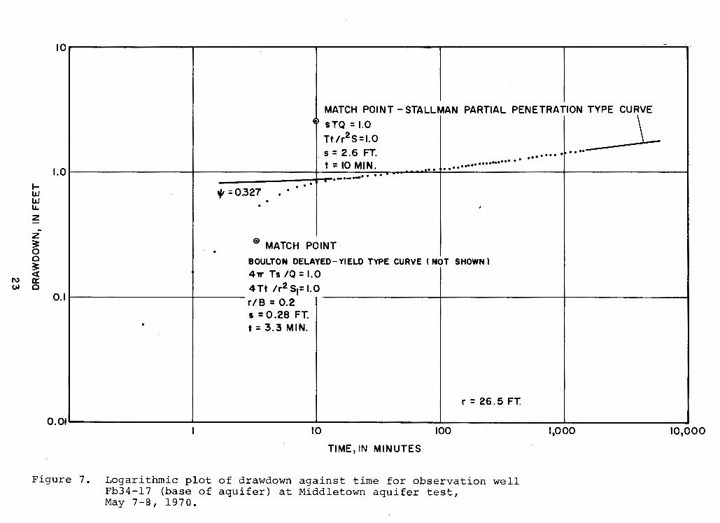
Figure 7 shows a logarithmic plot of drawdown againsttime for observation well Fb34-17 (r = 26.5 feet). Stallman(1965) has prepared type curves for analyzing drawdownsobserved in partially penetrating observation wells near apumped well penetrating the lower three-tenths of an aquifer.At the Middletown site, the pumped well is screened in thelower half of the aquifer and observation well Fb34-17 isscreened near the base,of the aquifer -- approximating theconditions of one of Stallman's models. As can be seen inFigure 7, the time-drawdown plot for observation wellFb34-17 exactly matches Stallman's type curve for $ = 0.327(Plate 7E in Lohman, 1972) from about 15 minutes to 1,440minutes (end of the test). Using the match point and asso­ciated parameters for Stallman's type curve, transmissiv~ty

is calculated as follows:

T = 1.0 Qs

T = (1.0) (60 gpm) (1,440 min/day)(2.6 f t.) (7.48 gal/ft 3

)

T = 4,500 ft 2/day or 33,000 gpd/ft

Using the same match point, storage coefficient is:

S = Tt

1.0 r 2

= (4,500 ft 2/day) (10 min)

(702 ft 2) (1,440 min/day)

S = 0.05 (rounded)

Spoljaric and Woodruff (1970, Figure 18) calculated a trans­missivity of 37,000 gpd by matching the later part of thetime-drawdown plot to the Theis artesian type curve. Thisvalue is not significantly different from the T calculatedwith the Stallman type curve. On the other hand, Woodruffcalculated a storage coefficient value of 0.006 which isless realistic for an unconfined aquifer than the S valuenoted above.

22

lor---------T----~----r---------r---------r---------=--.......I I I I - I

@ MATCH POINTI

BOULTON DELAYED-YIELD TYPE CURVE (NOT SHOWN),4.". Ts /Q =1.0

4 Tt /r2 Sf= 1.01...----------+-1---- r/ B =0.2 I 1 I I

s =0.28 FT.t =3.3 MIN.

....----. .

PARTIAL PENETRATION TYPE CURVE

\~.. . .. ..

MATCH POINT - STALLMAN~STQ=1.0 .

Tt /r2 S =1.0s =2.6 FT.t =10 MIN.

. ..'" =0.327

:- .Jj=.=.-----_ ...1.0

I-LLJLLJu,

2:~

2:3:003:<t

I\) ll::01 0

0.1

r =26.5 FT.

10 100 1,000 10,000

TlME,IN MINUTES

Figure 7. Logarithmic plot of drawdown against time for observation wellFb34-17 (base of aquifer) at Middletown aquifer test,May 7-8, 1970.

The time-drawdown plot was also matched againstBoulton's delayed-yield type curve (lower match point inFigure 7). The resulting value of transmissivity was some­what lower (25,000 gpd/ft) and S was about the same (0.04),as obtained from the Stallman type curve. Inasmuch asobservation well Fb34-l7 is only a short distance from thepumping well (about 0.6b), vertical flow components due topartial penetration and the effects of anisotropy in theaquifer are probably considerable. For this reason andbecause of the very close curve match, the values of T andS obtained in the Stallman type curve are considered to bethe most valid aquifer coefficients at the Middletown site.

Based on a saturated thickness of 42 feet and trans-missivity of 4,500 ft:/day, the horizontal conductivity(Kr) is 107 ft/day. Such a value is typical of medium tocoarse sand. The ratio of vertical to horizontal conduc­tivity (Kz/Kr) may be calculated with the parametersobtained from the match point on Stallman's type curve(Figure 6) as follows:

or

= PO.327) (42 ft)J2 =t 26.5 ft

0.25

Thus, the horizontal conductivity (Rr) is four times asgreat as the vertical conductivity (Kz), which is therefore27 ft/day. By comparison, at the Smyrna aquifer test site(Table 2), Kr is 10 times as great as Kz. At the Middletownsite, the aquifer is basically a coarse to medium sand inthe zone of saturation (see log in Spoljaric and Woodruff,1970, p. 118). However, at the Smyrna site, the aquifer isa coarse sand of high conductivity (200 ft/day) which isoverlain by beds of silty medium sand. Thus, the greaterratio of Kr to Kz at Smyrna seemS realistic. Conductivityratios are generally not available in published reports onthe Coastal Plain sand aquifers. However, for comparison,Weeks (1969) reported conductivity ratios of 2 to 20 forfive aquifer tests of glacial outwash in Wisconsin.

Milton aquifer test

The Milton aquifer test was made on the property ofMr. and Mrs. James H. Carpenter, about 3 miles southeast ofMilton, Del., as shown in Figure 1. The pumping well tapsone of the thickest known sand and gravel sections in

24

j ,

Delaware (see brief lithologic log in Figure 15). Further­more, as will be discussed in a later section, the drainingstream, Beaverdam Creek, has the highest base flow inDelaware. At the pumped well, Pleistocene fine to coarsesand extends to a depth of 50 feet and poorly sorted fineto coarse sand and gravel beds to a depth of 132 feet. Alower confining bed of clayey silt occurs from 132 to 150feet: however, the Miocene Manokin aquifer (medium to coarsesand) occurs below 163 feet. At the time of the aquifertest, the water table was 22 feet below land surface and thesaturated thickness of the Pleistocene deposits was, there­fore, 110 feet. The pumped well (Ng55-4) is screened nearthe middle of the aquifer (from 60 to 70 feet). One obser­vat ion well (Ng55-3), 98 feet away, is also screened nearthe middle of the aquifer (65 to 68 feet).

Well Ng55-4 was pumped for 48 hours and recoverymeasurements were made for 48 hours after the pumping period.A constant discharge of 198 gpm was maintained for 48 hoursusing the orifice method (variation less than 5 percent).The pumped water was discharged by irrigation pipe and aditch to Beaverdam Creek, about 1,200 feet from the site.

The measured drawdown in observation well Ng55-3 wassmall (1.32 feet) compared to the saturated thickness (110feet). Thus, no correction was needed to account fordewatering of the aquifer.

Figure 8 shows a logarithmic plot of drawdown againsttime for observation well Ng55-3. This plot can be closelymatched with Boulton's delayed-yield type curve riB = .2(Plate 8 in Lohman, 1972). As shown on Figure 8, the time­drawdown plot follows the delayed-yield type curve from 10to 1,000 minutes, and the later points closely follow theTheis artesian type curve. Using the match point andassociated parameters given in Figure 8, transmissivity (T)was calculated to be 14,000 ft 2/day (or 104,000 gpd/ft).Based on a saturated thickness of 110 feet, horizontal con­ductivity (Kr) is about 130 ft/day. This value is repre­sentative of coarse to medium sand (Lohman, 1972, Table 17)or "dirty" gravel.

The storage coefficient (8) was calculated to be 0.02,which is rather low for an unconfined aquifer. However,the fact that the late time-drawdown data ,closely match theTheis type curve suggests that delayed drainage was nearlycomplete and that the calculated 8 is valid.

25

10 i I I I I i

_-1__ -:-._....• •..

MATCH POINT G>

. ;:.;.. --............~ ......--.~ ~.".,..• .-- •• 1-.------",/'" ",I~THEIS ARTESIAN TYPE CURVE

./ './'

././

DELAYED-YIELD TYPE CURVE 1//

"rt Ir~ 5.= i.0 //

//

//

/

/

BOULTON DELAYED-YIELD TYPE CURVE riB =0.2 I _---I I __ ~ -.

4.". Ts IQ =1.0i 4 T ~. .

riB =0.2I =0.22 FT.t =4.3 MIN.

1.0

~1LIUJIL.

Z

..IZ

~00

I\) ~en Q:0 0.1

r =97.5 FT.

10 100 1,000

TIME, IN MINUTES

Figure 8. Logarithmic plot of drawdown against time for mid-aquiferobservation well (Ng55-3) at Milton aquifer test,Dec. 8-10, 1970.

Aquifer Coefficients Estimated by Reconnaissance Methods

Aquifer coefficients (transmissivity: T; storagecoefficient: S; and hydraulic diffusivity: TIS) were esti­mated by several reconnaissance methods. Transmissivity (T)was estimated from the specific capacity'of wells based ondrillers' reports. Transmissivity values also were estimatedfrom well logs by estimating values of hydraulic conductivity(K) for the materials penetrated. Storage coefficient (S)

was estimated by a hydrologic-budget technique involvingground-water level changes as compared to runoff and precip­itation. Hydraulic diffusivity (TIS) was estimated fromground-water level fluctuations using methods presented byRorabaugh (1960, 1966) and Stallman and Papadopulos (1966).

The advantages and disadvantages of these methods andtheir applicability to the Delaware Coastal Plain will bediscussed in a report, as yet unpublished, by the writer.The methods were used in the present study primarily toprepare a statewide map of the transmissivity of theColumbia deposits. The applicability of these methods forthis purpose is discussed briefly here.

Most of the values of transmissivity uSed to preparethe transmissivity map (Figure 9') were obtained fromspecific-capacity data. The specific-capacity data arebased on reported drawdowns in wells after short periods ofpumping (generally 2 to 8 hours)., Specific capacity wasconverted to transmissivity by equations and a chartpresented by Theis (1963) for water-table aquifers. Con­version factors used to compute T from specific capacityranged from 1,400 to 1,800 depending upon the well diameterand period of pumping. For example, specific capacityexpressed in gallons per minute per foot of drawdown, times1,500 equals transmissivity expressed in gallons per dayper foot of aquifer; gpd/ft. Transmissivity valuesobtained by this method, and by aquifer test analysis, arelisted in Table 7. Transmissivities calculated fromspecific capacity must be considered rough estimates. Inparticular, the length of well screen and well efficiencywere not considered in these calculations. However, morethan half the T values listed in Table 7, and shown inFigure 9, were obtained from fully penetrating large­diameter wells, and the efficiency of such wells would beexpected to be high initially. Where well efficiency ismuch less than 100 percent and the well screen penetratesa small part of the aquifer, the transmissivity values cal­culated from specific-capacity data will be erroneously low.However, no wells constructed with very short screens orwells with casing diameters less than 8 inches were used tocompute transmissivity. Specific capacity is discussed

27

further in the later section on the availability of water,and a frequency graph (Figure 13) of specific capacity forwells tapping the Columbia deposits is presented.

Transmissivity has been estimated from geologic logsof several test holes. In using this method, an averagehydraulic conductivity (K) is assigned to each lithologicinterval penetrated by the ,hole. The average K is multi­plied by the thickness of the interval and the sum of thesevalues provides an estimated T for the well. The values ofK used for this method are average values obtained from theaquifer tests listed in Table 2 as follows:

coarse sand with gravel beds. 250 ft/daysilty ("dirty") gravel. · . . 125 - 150 ft/daycoarse sand ~ 200 ft/day· . . · · · · · · . .coarse to medium sand · · · · 100 ft/dayfine to coarse sand · · · · · 50 - 75 ft/daymedium sand · · • · • 50 ft/dayfine sand . · . . · • • • 10 - 20 ft/day

These values of K are generally in agreement with K valueslisted in Lohman (1972, Table 17). Estimating T by thismethod is subject to considerable error because the methodinvolves the geologist's judgment of average effectivegrain size. For this reason, only a few values of Testimated from well logs were used to prepare the statewidetransmissivity map (Figure 9).

The values of transmissivity obtained from pumping-testdata, specific-capacity data, and estimates from geologiclogs are local values applying to a small segment of theaquifer. On the other hand, values of T obtained by methodsthat consider discharge from the aquifer to draining streams,as measured by water-level declines in wells, are averagevalues for a larger sample of the aquifer. The areal valuesof T are, of course, highly useful in preparing a statewidetransmissivity map.

Rorabaugh (1960) has shown that ground-water levelswill decline exponentially with time (after a critical timeperiod elapses), according to the hydraulic diffusiviti(T/S) of the aquifer and the square of the distance (a )from the draining stream to the ground-water divide. Valuesof T/S obtained by Rorabaugh's method are listed for severalwells in Table 3. The applicability of Rorabaugh's methodto the Coastal Plain of Delaware and a graphical example ofthe solution for T/S will be presented in a companion reportby the writer, as yet unpublished. In the case of wellMd24-1, listed in Table 3, there is close agreement betweenthe T/S value (175,000 ft 2/day) obtained with Rorabaugh's

28

method and the TiS value (170,000 ft 2/day) obtained usingthe transmissivity from the pumping test and long-termspecific yield (S = 0.13) listed in Table 3.

Stallman and Papadopulos (1966) have presented a methodfor determining TiS from the decline in water level at awell tapping a wedge-shaped aquifer drained by two streams.Values of TiS for two wells obtained with this method arelisted in Table 3. This method should be highly useful forevaluating the Pleistocene water-table aquifer. However,the method requires a continuous record of water-levelfluctuations in a well; whereas observation well data avail­able in Delaware are generally limited to monthly measure­ments.

Storage coefficient was estimated at several wells bymeans of simplified water-budget approach. The storagecoefficient (S) is considered to be equivalent to the long­term specific yield. Specific yield is generally definedas the change in the amount of water in storage per unitarea of aquifer that occurs as a result of a unit change inhead. However, the change in storage is gradual after achange in head in a water-table aquifer. This delayeddrainage causes specific yield calculated after a day or twoof drainage to be less than after several weeks or monthsdrainage. For this reason, the S values computed from shortaquifer tests (Table 2) are not representative of thespecific yield effective during long periods of aquiferdrainage (particularly the summer-fall period). The long­term specific yield was calculated for periods of soil­moisture surplus (winter periods), based on the assumptionthat all precipitation during such periods either enteredthe aquifer as recharge or left the area as stream runoff.Evapotranspiration is thus considered to be negligible.Actually some evapotranspiration does occur during thewinter months but the rates are less than 0.25 inch permonth during December, January, and February (Mather, 1969).

The simplified equation for computing specific yieldis as follows:

Runoff includes both direct runoff and ground-water runoff.In applying the equation, periods of 5 to 10 days followinga heavy rain were selected. The values of specific' yieldcalculated from the equation assume that delayed yield iscomplete at the end of the period. Also it assumed that thenet water-level change measured in an observation well isindicating the average net change in aquifer storage in the

29

TABLE 3 - Aquifer Coefficients Estimated by Reconnaissance Methods

wo

Well No.and

Location

Db24-l0(nearChristiana,Del. )

Hb14-l(nearBlackbird,Del. )

Md22-l(nearWilliams­ville, DeL; )

Md24-lnearHouston,Del. )

Ngll-l(nearMilton,Del. )

HydraulicDiffusivity

(T/S)(ft 2/day)

2,700

7,100

65,000

150,000

175,000

24,000

Transmissivity(T)

7,100 ft 2/day

54,000 gpd/day

r19,000 ft 2/day

lJ.45,000 gpd/ft

r2l,000 ft 2/day

1160,000 gpd/ft

3,400 ft 2/day

25,000 gpd/ft

StorageCoef­

ficient(S)

0.11

0.13

0.14

HydraulicConductivity

(K)

95 ft/day700 gpd/ft 2

Average K =230 ft/day

1,700 gpd/ft 2

70 ft/day500 gpd/ft 2

Remarks

Average T/S calculated byRorabaugh's method using water­level recessions in 1964 and1968. Thin saturated section(12 ft).

Average T/S calculated byRorabaugh's method using water­level recessions in 1963, 1964,and 1968. Thin saturatedsection.

Average T/S calculated byRorabaugh's method using water­level recessions in 1963, 1964,1965, and 1968. S calculated byhydrologic-budget method, using1967-69 water-level data.

T/S=150,000 ft 2/day by Stallman­Papadopulos method using 1970water-level data. T/S=175,000ft 2/day by Rorabaugh's methodusing 1970 water-level data.S=0.13 using hydrologic-budgetmethod

Average T/S calculated byRorabaugh's method using water­level recessions in 1963, 1964,1965, and 1968. S calculated byhydrologic-budget method using1969 water-level data.

Nc45-l 4,500 780 ft 2/day 0.17 10? ft/day Average T/S calculated by(near 5,800 gpd/ft Rorabaugh's method using water-Greenwood, level recessions in 1964 andDel. ) 1968. S calculated by hydro-

logic-budget method using1963-64 and 1966-67 water-leveldata. Anomalously low "T" con-firmed by driller's report.

Pf24-2 32,000 4,800 ft 2/day 0.15 64 ft/day T/S calculated by Stallman-(near 36,000 gpd/ft 540 gpd/ft 2 Papadopulos method using 1970Stockley, water-level data. S calculatedDe!.) by hydrologic-budget method

using 1970 water-level data.

area. The values of S obtained by this method range from0.11 to 0.17 and average 0.14. Values of S calculated bythis method as well as values of T/S and T calculated withthe Rorabaugh and stallman-Papadopulos methods are listed inTable 3.

Areal Distribution of Transmissivityand Hydraulic Conductivity

Figure 9 shows the distribution of transmissivity (T) inthe Columbia deposits throughout Delaware. The map is basedprimarily on transmissivity values estimated from the specificcapacities of large-diameter wells. Accurate control pointswere provided by the T values obtained from the aquifer testsand the T values obtained by analyses of water-level reces­sions (using the methods of Rorabaugh, 1960 and Stallman­Papadopulos, 1966). A few transmissivity values estimatedfrom geologic logs are shown on the map. However, becausethese estimates were highly subjective, only a few such Tvalues are shown.

Because of the spotty nature of the well data, a rela­tively large interval of 5,000 ft 2/day is shown for the linesof equal transmissivity in Figure 9. It is readily apparentfrom the map that large changes in T occur in relatively shortdistances. These changes in T reflect changes in lithology(from fine to medium sand to coarse sand and gravel, forexample) as well as changes in saturated thickness. Comparisonof the transmissivity map with the saturated aquifer thicknessmap (Figure 3) indicates a general increase in transmissivityand saturated thickness from north to south across Delaware.

Six areas have been outlined on Figure 9 where thetransmissivity is known to exceed 10,000 ft 2/day (75,000gpd/ft). Within these areas, transmissivities are as much as170,000 gpd/ft (22,000 ft 2/day). The highest transmissivitiesdo not necessarily correspond to the sites of thickest satu­rated section.

Four of the high transmissivity areas occur in thefluvial facies of the Pleistocene aquifer -- north of apresumed former shoreline, which Jordan (1964) postulated asextending along "a west-southwest axis running roughly fromLewes through Seaford." These high T areas are most likelyunderlain by stream channel deposits and the transmissivitiesindicate that the average effective grain size is about thatof a coarse sand. Comparison of the structure contour map onthe base of the Pleistocene (Figure 2), the saturated thick­ness map (Figure 3), and the transmissivity map (Figure 9)suggests that:

31

l5'45' 11'30' /S'I!'

.IS4lO4100

llOGe:FIAIUlIIlIIIlIII

EXPLANATION

-10,000----

LINE OF EQUAL TRANSMISSIVITY.DASHED WHERE APPROXIMATELYLOCATED. INTERVAL; e.ooo FEETSQUARED PER DAY.

TRANSMISSIVITY VALUES INFEET SQUARED PER DAY.

10TE:TRAISIISSIVITl II FEET SQUAREll P9 DATlFT;DA!1IlILTlPllED ., 1I EQUAlS TRAISIII$IVITl •GAUOIS PElDA' PER FOOT (;po/Fn. AlII ElMlPlE10.000 fTl/DA' • 'S,OOO GPDIFT.

SOURCE OF TRANSMISSIVITY VALUE:

• ANALYSIS OF AQUIFER TEST DATA

o ESTI MATEO FROM SPECIFIC CAPACITY DATA

C ESTIMATED FROM WATER LEVEL FLUCTUATIONS

• ESTIMATED FROM WELL LOGS

JERSEY

SUSSEX

COUNTY

·3100

oZ:De-...1'00 °SIOD O~_

o 8,000-­4200

COUNTY

1100•

o3300

KENT

\ ITOO~SEAFOR1l1 1400 2100 3000

1\ 0 5TOO;:OO

~O.IIO

\ IO.DOO\\.~'~IUREl

\

21.oao ~-' ~

1000 11000\ Iz.o:O,I ) 13.000 \I / • \ ._

I / 44110' .10.000L--__ ---SL..:_____. lIDD!!SllfLITWlW ...Illl.. ---------- -------

I

\1I

t--~--:~\ ao O·I1

II

\

" \._"-~/_ 4y-- -~~..

~y CRYSTAU.INE ROCKS

,

;'

31'30'

FIGURE 9. TRANSMISSIVITY MAP OF THE COLUMBIA (PLEISTOCENE) DEPOSITS INDELAWARE.

(1) The high transmissivity area at Smyrna ispart of a southeast trending channel whichmay turn eastward and include the high Tarea northeast of Dover.

(2) The high transmissivity area at Milton mayinclude two channels which coalesce andhead northeast along the present-day courseof the Broadkill River.

(3) The high transmissivity area betweenHarrington and Milford may possibly be partof a southeast trending channel (or channels).

Two of the high transmissivity areas occur in the near­shore (beach, estuarine, neritic, and lagoonal) facies of theColumbia deposits. Correlation of the high T areas with theindividual facies is rather tenuous. The high transmissivityarea south of Laurel may be related to very thick Pleistocenechannel fill deposits just south of the Delaware state line-- about 2 miles north of Salisbury, Maryland. As mapped byHansen (1966), this so-called paleochannel contains sand andgravel attaining a maximum thickness of 220 feet. Morerecently, Weigle (1972) has mapped a tributary channel extend­ing northward toward the Delaware line just east of Delmar.If extended, this channel would intersect the l83-foot valueshown southeast of Laurel on the saturated thickness map(Figure 3). Actually all the area south of Seaford (includ­ing Laurel) to the Maryland line is characterized by a verythick saturated section and above average transmissivity.The area is probably a complex mixture of beach sand andstream channel deposits which can only be delineated by muchexploratory drilling.

Some of the transmissivity values shown for southeasternDelaware (Figure 9) seem to be anomalously low in view of thefact that the saturated thickness in that area generallyexceeds 75 feet. However, as mapped by Jordan (1962), alarge part of southeastern Sussex County is underlain by finesand and silt which Jordan termed the Qmar Formation. Thesesand and silt beds could be expected to have hydraulic con­ductivities of less than 10 to 20 ft/day. Rasmussen andothers (1960) applied the terms "Pamlico and Talbot Forma­tions" and "Walston silt" to describe these fine sands andsilts. Owens (oral communication, Oct. 1972) considers thesefine-grained sediments as part of a "back barrier facies"which occur in a continuous narrow belt extending from south­eastern Delaware to Virginia parallel to the coastline. Inany case, below average values of transmissivity can beexpected in parts of southeastern Delaware where these fine­grained deposits make up a sizable part of the saturatedsection of the Pleistocene deposits.

33

Laboratory determinations of hydraulic conductivity, asreported by Rasmussen and others (1960), indicate largevariations in values. Samples collected from shallow pitshad conductivities ranging from less than 1 to about 200 ft/day. Samples collected from well Qd2l-2 at Laurel (in thehigh transmissivity area) had conductivities ranging from125 to 500 ft/day.

The average transmissivity (T) of the Columbia depositsis about 7,000 ft 2/day (53,000 gpd/ft) in central andsouthern Delaware (based on T values shown in Figure 9).Within this area, the average saturated thickness of theaquifer is about 75 feet and, therefore, the average hydraulicconductivity (K) is about 90 ft/day. Such a K value is char­acteristic of medium t9 coarse sand. Jordan (1964) also con­cluded that the Columbia deposits are mainly medium sand,based on geologic studies. Therefore, both the geologicstudies and hydraulic data support the conclusion that theColumbia deposits are effectively a medium to coarse sandaquifer.

In those parts of Delaware where the Columbia depositsare known to consist of medium or medium to coarse sand, ahydraulic conductivity (K) of 50 to 100 ft/day may be assumed.In areas where the aquifer is mostly "clean" coarse sand andinterbedded gravel (as at the Houston and Smyrna aquifer testsites), K can be assumed to be 200-250 ft/day. In areaswhere the aquifer is predominantly coarse sand (as at Lewes)or "dirty" gravel (as at the ~ilton test site), the averageK can be assumed to be 100-150 ft/day.

GROUND-WATER HYDROLOGY

The Columbia deposits are part of an interdependentstream-aquifer system in the Delaware Coastal Plain. TheColumbia deposits comprise the uppermost and most permeablesection of saturated sand in the water-table aquifer through­out most of Delaware. In fact, the water-table aquifer iscomposed essentially of Columbia (Pleistocene) "deposits inabout 75 percent of Delaware (1,500 square miles). ThePleistocene deposits receive most recharge reaching the watertable and are the outlet for most ground-water discharge.

The small Coastal Plain streams are incised into theupper part of the Columbia deposits and derive much of theirflow (50-90 percent) from ground-water runoff. Except forperiods of overland runoff, these streams act as shallowdrains from the aquifer. precipitation and evapotranspirationrates determine the recharge rate to the aquifer and, in turn,

34

changes in storage in the aquifer closely control base flowof the draining streams. The rate at which the aquifer dis­charges water to the draining streams is also influenced bythe aquifer's hydraulic characteristics (Johnston, 1971).

Underlying the Columbia deposits of central andsouthern Delaware are Miocene deposits which contain severalsand aquifers. In much of ,the area, the Miocene sands areseparated from the Columbia deposits by confining beds ofsandy clay. Locally there are small differences in hydraulichead between the Columbia and Miocene aquifers. However, thequantity of leakage is considered to be very small relativeto the recharge and discharge to streams from the Columbiadeposits.

The following section will consider changes in storagein the Columbia deposits, and by analysis of base flow data,present estimates of recharge to and discharge from theColumbia deposits.

Changes in Storage (Water-level Fluctuations)

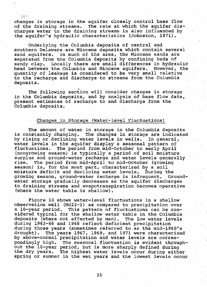
The amount of water in storage in the Columbia depositsis constantly changing. The changes in storage are indicatedby rising or declining water levels in wells. In general,water levels in the aquifer display a seasonal pattern offluctuations. The period from mid-October to early April(nongrowing season) is typically a period of soil moisturesurplus and ground-water recharge and water levels generallyrise. The period from mid-April to mid-October (growingseason) is, for the most part, characterized by a soilmoisture deficit and declining water levels. During thegrowing season, ground-water recharge is infrequent. Ground­water storage gradually decreases as the aquifer dischargesto draining streams and evapotranspiration becomes operative(where the water table is shallow).

Figure 10 shows water-level fluctuations in a shallowobservation well (Md22-l) as compared to precipitation overa 10-year period. This pattern of fluctuations can be con­sidered typical for the shallow water table in the Columbiadeposits (where not affected by man). The low water levelsduring 1962-66 and 1968 reflect deficient precipitationduring those years (sometimes referred to as the mid-1960'sdrought). The years 1967, 1969, and 1971 were characterizedby above-normal precipitation and water levels are corres­pondingly high. The seasonal fluctuation is evident through­out the 10-year period, but is more sharply defined duringthe dry years. The highest water levels occur during eitherspring or summer in the wet years and the lowest levels occur

35

OBSERVATION WELL Md 22-10

ILl0 • .

~c( .\ • • \ • 1\ •....IlL • I \ I' !\1\ILIa: 1\ , I· \ i\ I>;:) • , . ,\ / .lLIeI) I ., I • • • • • t, ,\j .,. : •• /I • • • \ 1\....10 5 . , \ 1\ 1 \1 " \ I \ , ~, • \, \!a: Z I •• I .. \ ••1LIe( • \ \ I \ I· • • I ,. v : \/~....I

, \,

• , • • \ ! ~, \ I \/e(~ I • , , , \ I \ ,\~o

, , \ /I • I· \,.

0....1 • I • \ , • \ \ I I\ . • I •~ILI ', I •../ • • • • I \ •III ,:J:~ 10 • • I • I ,,. •~ILI ../ •.. / • ..,.Q. ILI •~IL.

Z

Ie' I I , " I I I 'I I , " " I I I I I I , I , I 'I , I , , I I , I I I " " I I , I , I I I , I I I , I I I , I , I I " I " , I , I , I , I I , «' I I I I I I I I I I « I , I I I I I I '" I I I I I , , , , I , , , , , , , I

01en

1962 1963 1964 1965 1966 1961 1968 1969 1910 1971

ANNUAL PRECIPITATION, IN INCHES:

37.5 39.3 34.6 28.6 31.? 48.9 28.1 54.8 40.2 41.6u) 20ILl:J:o .z....I- ILl 15z~-0zl:2:2 10lii~~2

ii: ... 5oe(ILla:Q.

01962 1963 1964 1965 1966 1961 1968 1969 1910 1971

Figure 10. Hydrograph of water level in shallow observationwell Md22-1 and precipitation at Milford, Del. ,1962-1971.

in the fall of the dry years (1965 and 1968, for example).However, no long-term decline or rise in the water table isapparent.

The saturated thickness of the aquifer at well Md22-lis 70 to 80 feet. Thus, the seasonal water-level fluctua­tions indicate a change of about 10 percent of the water instorage in the aquifer. In northernmost Kent County andmost of New Castle County, where the saturated thickness isless than 25 feet, seasonal fluctuations of the water tablechange the amount of water in storage by a greater percent­age. In eastern and southern Sussex County, where thesaturated thickness exceeds 100 feet, seasonal water-levelfluctuations change the amount of water in storage by approx­imately 5 percent.

Changes in storage in the aquifer, as measured by waterlevels in a specific well, are caused by several factorsincluding:

(1) Location of the well with respect to theground-water divide and the draining stream(wells close to the divide show largerwater-level fluctuations and wells close tostreams show smaller fluctuations).

(2) Hydraulic characteristics of the aquifer,particularly the hydraulic diffusivity (T/S).

(3) Thickness and character of the unsaturatedzone (which influences the rate and timingof recharge).

(4) Relation.of water-table altitude to artesianheads in underlying aquifers.

Figure 11 shows hydrographs of water levels in fourobservation wells, representing different combinations of thehydrologic factors cited above. The locations of these wellsare shown in Figure 1.

The uppermost hydrograph (Md24-l) shows water-levelfluctuations in an area characterized by a relativelyshallow water table and a sand and gravel aquifer of veryhigh transmissivity and diffusivity (T = 22,000 ft 2/day andT/S = 180,000 ft 2/day). Infiltration is apparently rapidand, during the winter and spring, water levels begin risingwithin a few hours after the start of a heavy rain.

Well Md24-l is relatively close to the draining stream(1,200 feet away), and part of the rise may be due to bank-

37

OBSERVATION WELLMd24-1

SHALLOW WATER TABLEIN SAND AND GRAVEL OF

VERY HIGH TRANSMISSIVITY.

7.0,..

6.0 ,..

5.0,..

3.0.....-------------------------------------,/.\

I •. \ /.,/. I \ I

4.0"'! \ 1 • \ • ...._., • I' •\ \ \ I

• /., , \ I •\ \1· \ }, I • \ ",.· l ., i" \ I\, .

\ ......\ I \ .\ 1\ •• • I 1• I "'. • •\. 1 \./

'\ ,·,1

•

OBSERVATION WELLPf24-2

AVERAGE DEPTH TOWATER TABLE IN SANDSOF AVERAGE TRANSMISS­IVITY.

II.O~

8.0L.--------------------------------------'

8.0.....------------------------------------....../ ..... j\ ;\• \ , I '.

9.0- 1\ j · \ /\ ' -.__.• I • • • ,\ \I I\. . ., \ 1 ' ......

10.0 - \ i . I.... I \ •

•\ I J~. ~.. /'. ......'-./

21.0'"

22.0f-

23.0

OBSERVATION WELLNg55-3

WATER TABLE AT ABOVEAVERAGE DEPTH IN SANDAND GRAVEL OF ABOVEAVERAGE TRANSMISSIVITYWITH SUBCROPPINGMIOCENE AGE MANOKINAQUIFER.

30.0.....--------------------------------------,OBSERVATION WELL

Fb34-17

DEEP WATER TABLE INSANDS OF AVERAGETRANSMISSIVITY WITHSUBCROPPING PALEOCENEAND EOCENE AGERANCOCAS AQUIFER.

34.0 I I I I I

J A SON

1970

I I I I

D J F MI I I I I I I I I

AMJ JASOND

1971

Figure 11. Hydrographs of water levels in fourobservation wells tapping theColumbia deposits under differenthydrogeologic conditions.

38

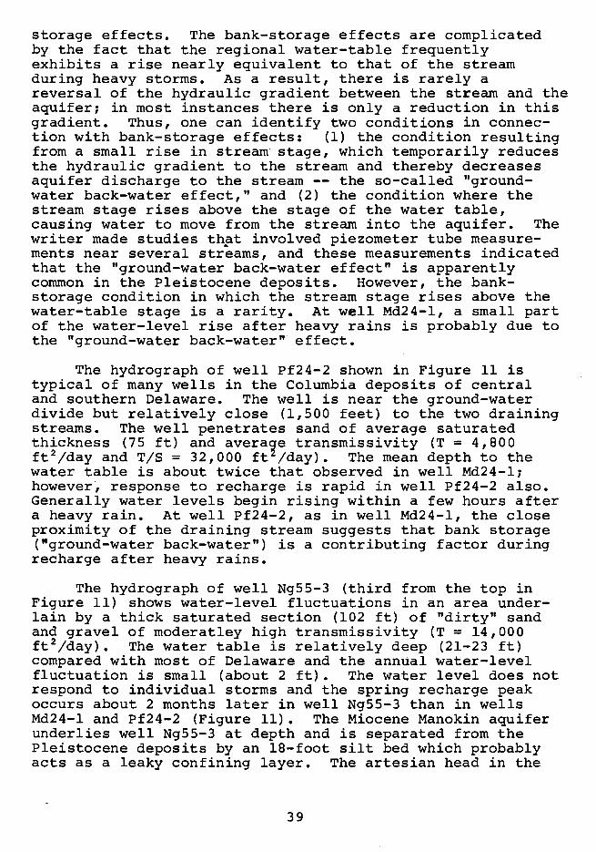
storage effects. The bank-storage effects are complicatedby the fact that the regional water-table frequentlyexhibits a rise nearly equivalent to that of the streamduring heavy storms. As a result, there is rarely areversal of the hydraulic gradient between the stream and theaquifer; in most instances there is only a reduction in thisgradient. Thus, one can identify two conditions in connec­tion with bank-storage effects: (1) the condition resultingfrom a small rise in stream stage, which temporarily reducesthe hydraulic gradient to the stream and thereby decreasesaquifer discharge to the stream -- the so-called "ground­water back-water effect," and (2) the condition where thestream stage rises above the stage of the water table,causing water to move from the stream into the aquifer. Thewriter made studies thpt involved piezometer tube measure­ments near several streams, and these measurements indicatedthat the "ground-water back-water effect" is apparentlycommon in the Pleistocene deposits. However, the bank­storage condition in which the stream stage rises above thewater-table stage is a rarity. At well Md24-l, a small partof the water-level rise after heavy rains is probably due tothe "ground-water back-water" effect.

The hydrograph of well Pf24-2 shown in Figure 11 istypical of many wells in the Columbia deposits of centraland southern Delaware. The well is near the ground-waterdivide but relatively close (1,500 feet) to the two drainingstreams. The well penetrates sand of average saturatedthickness (75 ft) and avera~e transmissivity (T = 4,800ft 2/day and T/S = 32,000 ft /day). The mean depth to thewater table is about twice that observed in well Md24-l;however, response to recharge is rapid in well Pf24-2 also.Generally water levels begin rising within a few hours aftera heavy rain. At well Pf24-2, as in well Md24-l, the closeproximity of the draining stream suggests that bank storage("ground-water back-water") is a contributing factor duringrecharge after heavy rains.

The hydrograph of well Ng55-3 (third from the top inFigure 11) shows water-level fluctuations in an area under­lain by a thick saturated section (102 ft) of "dirty" sandand gravel of moderatley high transmissivity (T = 14,000ft 2/day). The water table is relatively deep (21-23 ft)compared with most of Delaware and the annual water-levelfluctuation is small (about 2 ft). The water level does notrespond to individual storms and the spring recharge peakoccurs about 2 months later in well Ng55-3 than in wellsMd24-l and Pf24-2 (Figure 11). The Miocene Manokin aquiferunderlies well Ng55-3 at depth and is separated from thePleistocene deposits by an l8-foot silt bed which probablyacts as a leaky confining layer. The artesian head in the

39

Manokin is unknown at well Ng55-3, but the head is probablyhigher than the water-table altitude (8-10 ft above mean sealevel). Probably there is substantial leakage from theManokin (which obtains recharge some distance away) into thePleistocene sand, thus explaining the 2-month delay inrecharge response. Furthermore, the water level in wellNg55-3 displays barometric fluctuations (more typical of anartesian aquifer than the unconfined Pleistocene sand),suggesting hydraulic connection with the Manokin aquifer.

The lower hydrograph in Figure 11 shows water-levelfluctuations in well Fb34-l7 which taps a 42-foot thicksaturated section of Pleistocene sand of average transmis­sivity (T = 4,500 ft 2/day). The water table at the well isexceptionally deep (30-33 ft) for the Delaware Coastal Plain.Directly underlying tha Pleistocene sands are "greensands"of the Paleocene and Eocene Rancocas aquifer and the twoaquifers are probably hydraulically connected. As shown inFigure 11, the normal October water-level rise (as seen inwells Md24-l and Pf24-2) did not occur in well Fb34-l7 untilMarch, 1971. Furthermore, during the wet year of 1971, thenormal summer water-level decline is almost nonexistent, andthe water level shows a generally rising trend throughout theyear. The combination of a thick unsaturated zone (whichdelays recharge) and hydraulic connection with the Rancocasaquifer (which may be receiving recharge at some distance) isprobably responsible for the water-level trend seen inFigure 11.

Well Fb34-l7 does not show the normal seasonal water­level fluctuations but, rather, is responding to long-termchanges in precipitation. The year 1970 was characterizedby below-normal precipitation (34 inches at Middletown),whereas 1971 was characterized by exceptionally high precip­itation (56 inches), and the~changes in ground-water storageobserved in well Fb34-l7 simply reflect this year-to-yeardifference.

Ground-Water Discharge

Ground-water discharges continuously from the Columbiadeposits to the small streams draining the Delaware CoastalPlain as well as directly to the Delaware Bay and AtlanticOcean. A small amount of ground water also evaporates andtranspires. That part of the streamflow supplied by ground­water discharge is referred to as ground-water runoff.During periods when a stream is supplied largely by ground­water discharge, it is said to be at base flow. Actually,the small nontidal streams in the Delaware Coastal Plain aresupplied entirely by ground-water seepage during base-flow

40

conditions (Johnston, 1971). After a rainless period of afew days, base-flow conditions prevail and the total dischargeof a stream represents ground-water runoff. However, ground­water runoff persists during periods of heavy rainfall andmay, in fact, be higher than during later periods of baseflow (Figure 12).

At streams where continuous gaging stations are operated,it has been possible to determine ground-water discharge byseparation of the streamflow hydrographs into the componentsof ground-water runoff and overland runoff. Determination ofground-water runoff from streamflow hydrographs assumes thatthe gaging station is measuring the total runoff from thebasin. In most cases this is true. However, discrepanciesmay occur between the ~easured runoff and the actual runoffbecause of either man-made effects such as withdrawal ofwater and operation of dams, or natural effects such as move­ment of ground water into or out of deep artesian aquifers.By selecting basins where the man-made effects are known tobe minimal and where inter-aquifer movement of water isnegligible, a fairly accurate estimate of ground-water runoffcan be made by hydrograph separation. Assuming that the rateof ground-water discharge is the same in the gaged areas asin the ungaged areas (including tidal streams and areas dis­charging directly to the Delaware Bay and the ocean), it ispossible to estimate the total ground-water runoff from thewater-table aquifer.

As mentioned in an earlier section, the water-tableaquifer consists largely or entirely of the Columbia depositsthroughout an area of abou~ 1,500 square miles in Delaware.The ground-water runoff of the streams draining this 1,500square mile area, therefore, represents the ground-water dis­charge minus evapotranspiration from the Columbia deposits inDelaware.

The streamflow hydrographs were separated into theground-water and overland-runoff components by using a masterbase-flow recession curve as described by Riggs (1963).Preparation of the base-flow recession curves and the assump­tions upon which they are based, are discussed in an as yetunpublished report by the writer.

Figure 12 shows an example of hydrograph separation forStockley Branch -- a small stream in southern Delaware(Figure 1). In making the separ~tion, the master recessioncurve is superimposed on the streamflow hydrograph at thebest fit~ all streamflow above the curve is considered over­land runoff, whereas all flow below the curve is ground-waterrunoff. The segments of the master recession curve used to

41

A. GROUND-WATER LEVEL IN OBSERVATION WELL Pf 24 -2, STOCKLEY, DEL.

50J---------+--------+-----'------+--------1---------1

---GROUND-WATER RUNOFF

5 10

'IGURE: 12. GROUND-WATER RUNOFF AND OVERLAND RUNOFF AT STOCKLEY BRANCHCOMPARED TO GROUND-WATER LEVELS, MAY- SEPTEMBER 1971.

42

......... /"> . -.,., • ">,1.-...! ...........,

i .,<,

-:..... .-.-................. ( .--

.......<,.......... .. r -.-... I

-I '.--. •-. /............

.11.5

12.0

8.0

IIIII~»t.

I ~ 20J-----4i-----+--------+--------+--------il--I---------1

~IIJ

I~iii ' 10.----E::::::=r---e,..---------+--------+-------~t----f:::*----1

I~

IIfitQ

IIII

I ~ 8.5.~

.J a: 9.0

~~a: z 9.5

~~ 10.0

~~

~~ 105

o u, 11.0z

make the separation are shown by dashed lines in the stream­flow hydrograph in Figure l2(B). The master curve is movedsideways on the streamflow hydrograph after each ground-waterrecharge event. These events are indicated by periods ofrising ground-water levels, as shown in the observation wellhydrograph in the upper part of Figure 12. The peak ground­water stage during such recharge events is assumed to coin­cide with a ground-water-runoff peak. The observation wellin this case is about 1,500 ft from Stockley Branch and is agood indicator of changes in ground-water storage.

As discussed earlier, rises in ground-water levels mayresult not only from recharge but also from bank storage(the so-called "ground-water back-water effect"). However,bank-storage effects are probably minimal at well Pf24-2,which is about 1,500 ft from the stream. This is indicatedby the fact that during some of the overland-runoff peaksseen ~n Figure 12 (July 2 and 19, 1971, for example), thereis no corresponding rise in ground-water level.

During periods of heavy overland runoff and frequentrecharge to the water-table aquifer (particularly during thewinter and spring), rating curves of base flow againstground-water stage were used t~estimate ground-water runoff.Such curves are presented and discussed in another report bythe writer, as yet unpublished, on ground water-surface waterrelations. The relationship between ground-water stage andbase flow is variable, however, being dependent upon thecurrent evapotranspiration rate and time since last recharge(see papers by Rorabaugh, 1960 and 1966). For example, asshown in Figure 12, on July 5, a ground-water level of 9.75feet was equivalent to a base flow of 3 cfs (cubic feet persecond), whereas on September 25 a similar stage of 9.75 feetwas equivalent to a base flow of about 4 cfs. Presumably thehigher evapotranspiration rate in July is responsible for thelower base flow occurring at the same ground-water stage asthe higher base flow in September. Also, the base flow onSeptember 25 closely followed a time of recharge and ground­water levels were declining at a faster rate than on July 5,a month after the last recharge (see Rorabaugh, 1960 and196~). Both the master recession curves and ground-waterstage base flow rating curves are approximations. However,the estimates of ground-water runoff obtained by use of thesecurves are probably accurate within 10-15 percent.

Ground-water runoff was determined for six streamsdraining the Pleistocene aquifer by the same method describedfor Stockley Branch. The drainage areas, average discharges,and ground-water runoff of these six streams are listed inTable 4. The 3-year period (1968-70) was selected for deter­minations of ground-water discharge because precipitation was

43

TABLE 4 - Streamflow and Ground-Water Runoff from Six Basinsin Central and Southern Delaware

Drainage Areas StreamflowGround-Water Runoff

Stream and (1968-70)location Surface Ground-water Average Average Average Averageof gaging drainage basin discharge discharge ground-water ground-waterstation area area (long term) (1968-70) runoff runoff

(mi 2) (mi 2) (cfs) 1/ (cfs) (winter period)

Beaverdam 2.82 2.85 3.49 3.72 2.91 cfs 3.50 cfsBranch at (12 years) (1.02 cfsm) 2/ (1.23 cfsm)Houston, Del.

Murderki11 13.6 15.6 17.4 I 20.3 10.7 cfs 13.7 cfsRiver near (12 years) (0.69 cfsm) (0.88 cfsm)Felton, DeL

Nanticoke 75.4 72.5 90.6 9L6 76 cfs 86 cfsRiver near (27 years) (1.05 cfsm) (1.19 cfsm)

,j:>,Bridgeville,

,j:>, Del.

St. Jones 31.9 31.5 29.8 31.5 16.1 cfs 23.3 cfsRiver at (12 years) (0.51 cfsm) (0.74 cfsm)Dover, Del.

Sowbridge 7.08 8.0 9.55 8.38 6.57 cfs 7.37 cfsBranch near (14 years) (0.82 cfsm) (0.92 cfsm)Milton, Del.

Stockley 5.24 5.6 6.89 6.09 4.84 cfs 5.90 cfsBranch at (27 years) (0.86 cfsm) (1.05 cfsm)Stockley, Del.

Totals 136.0 136.0 157.7 161.6 117.0 cfs 139.8 cfs

Mean - - - 1.19 cfsm 0.86 cfsm 1.03 cfsm

1/ Cubic feet per second

~ Cubic feet per second per square mile

near normal and streamflow was about average during the 3years. As shown in Table 4, the combined average dischargefrom the six basins was 161.6 cfs during 1968-70 comparedwith 157.7 cfs for the period of record at the six gagingstations.

Observation well data were available in four of the sixbasins listed in Table 4, ,and it was possible to obtain areasonably accurate determination of ground-water runoff fromthe streamflow hydrographs. However, for two of the sixstreams (St. Jones River and Murderkill River), observationwell data were unavailable and the base flow values listed inTable 4 are estimates. During the long summer-fall base flowrecession, these estimates are reasonable accurate. However,during periods of considerable overland runoff and frequentground-water recharge·(winter and spring), the ground-waterrunoff values for these two streams are only rough estimates.

Note that the drainage areas used to calculate ground­water runoff per square mile are the areas of the ground­water basin (as determined from water-table maps) and not thesurface-drainage areas. However, although the surface- andground-water drainage areas of individual basins may varyconsiderably, the total surface- and ground-water drainageareas for the six streams are the same (136 square miles).

The average ground-water runoff of the six streamslisted in Table 4 is 0.86 cfsm (cubic feet per second persquare mile), or 550,000 galjdayjsq mi (gallons per day persquare mile), as compared with the average discharge (1.19cfsm). Ground-water discharge, therefore, constitutes about72 percent of the total flow of these streams. Using theaverage ground-water runoff rate of 550,000 galjdayjsq mi,the total ground-water discharge from the Columbia depositshas been estimated. This estimate is based on the followingassumptions:

(1) Ground-water runoff occurs at the same ratein the ungaged areas as in the six drainagebasins listed in Table 6.

(2) Direct outflow to the Delaware Bay andAtlantic Ocean, which could not be determineddirectly, also occurs at the same rate asground-water runoff in the six basins.

These assumptions are considered plausible because long-termrates of precipitation and evapotranspiration are similarthroughout the 1,500 square miles where the Columbia depositsconstitute the water-table aquifer. Also, the aquifer char­acteristics in the six basins are typical of the 1,500 square

45

mile extent of the Columbia deposits in Delaware. Based onthese assumptions, the average ground-water discharge fromthe Columbia deposits in Delaware is about 800,000,000 gallday (or 800 mgd).

After reaching the water table and before discharge fromthe Columbia deposits, some water moves into and out of theunderlying Tertiary artesian aquifers. Locally, the amountof this leakage may be considerable (see, for example, thediscussion of Beaverdam Creek basin in the later section onthe availability of large water supplies). However, suchleakage does not change the estimate of discharge given abovebecause the Columbia deposits are the final discharge outlet.

~

Ground-Water Recharge

Recharge to the Columbia deposits takes place primarilyduring the nongrowing season from about mid-October to earlyApril. During this period, frequent pulses of rechargegradually raise ground-water levels as well as the base flowof streams. Throughout the growing season, from April tomid-October, recharge is less frequent. A soil-moisturedeficit exists much of the time and ground-water levelsgradually decline. Heavy rains resulting from thundershowersand tropical storms are occasionally sufficient to overcomethe soil moisture deficiency and to provide surplus waterwhich infiltrates to the water table. Figure 10, showing the10-year hydrograph of ground-water levels in shallow observa­tion well Md22-l, illustrates the typical pattern of recharge.Except for the wet summers of 1967 and 1969, nearly allrecharge occurred during the winter.

Over the long term, there has been no change in theamount of water in storage in the Columbia deposits, as notedpreviously. Therefore, the long-term average recharge rateis equal to the discharge from the aquifer. Inland from thecoast, the discharge is the sum of the ground-water runoffand ground-water evapotranspiration.

The average rate of recharge is difficult to determineat a given site. Some investigators have determined rechargeby multiplying the average specific yield of an aquifer bythe net water-table rise during a long period of time (see,for example, Rasmussen and Andreasen, 1959). However, thismethod requires a large number of observation wells locatedin areas characterized by different infiltration rates.Furthermore, specific yield is dependent upon time and othervariables and estimates of the average effective specificyield are problematical. The effective specific yield duringa period of recharge will also depend upon the moisture

46

content above the water table at the time of recharge, whichvaries according to the time since the previous period ofrecharge. This time factor in the effective specific yieldis influenced by the particle size and other variables. Inaddition, the rise in ground-water levels observed in a wellmay include bank-storage components as well as ground-waterrecharge.

Although recharge occurs primarily during the winter,there is little difference between the mean ground-waterstage during the summer and winter. A hydrograph showingthe average depth to water level in 13 water-table wells inDelaware has been presented by Boggess and others (1964) forthe l2-year period, mid 1950 to July, 1962. During thesummer (May-September), the mean depth to water level isslightly lower (0.46 foot) than during the winter (November­March). This small difference is probably caused by evapo­transpiration directly from the aquifer. Shallow observa­tion wells in the Beaverdam Branch, Nanticoke River, andStockley Branch basins (listed in Table 4) are characterizedby summer water levels averaging 0.2 to 0.4 foot lower thanin the November-March period. However, a shallow well justoutside Sowbridge Branch basin (also listed in Table 4) ischaracterized by a mean summer water level about 0.6 foothigher than the mean winter water level. The reason for thehigher summer water level may be the relatively low hydraulicdiffusivity (TiS) in the basin, which results in slow drain­age of the Pleistocene deposits in the summer and perhaps isdue also to upward leakage from the Miocene deposits duringthe summer. These explanations are conjectural and, in anycase, the observation well near the Sowbridge basin isatypical of those tapping the Columbia deposits.

Inasmuch as the ground-water discharge varies directlywith ground-water stage, the ground-water discharge duringthe summer (ground-water runoff plus ground-water evapo­transpiration) is not 'substantially less than the ground­water discharge during the winter (all ground-water runoff).Because there has been no long-term change in ground-waterstorage, the long-term rates of ground-water discharge andrecharge are equal. Based on the premise that the winterand summer rates of ground-water discharge are similar, theground-water runoff during winter is approximately equal tothe average year-round recharge rate. Note that a largepart of the recharge during the winter is carried over inaquifer storage and later discharged during the summer. Thesmall amount of summer recharge provides only part of thesummer ground-water runoff and evapotranspiration.

The average rate of recharge in the 1,500 square milearea where the Columbia deposits constitute the water-table

47

aquifer, is assumed to be the same as in the 136 square milearea drained by the six streams listed in Table 4. Withinthis 136 square mile area (where the difference between themean summer and winter ground-water levels is less than 0.4foot), the average rate of ground-water recharge is approx­imately equivalent to the ground-water runoff during thewinter. The average recharge is, therefore, approximately1 cfs per square mile or 650#000 gallons per day per squaremile. The total recharge to the Columbia deposits throughoutits 1,500 square mile extent in Delaware is, thus, about 1billion gallons per day.

GROUND-WATER DEVELOPMENT.Yield and Specific Capacity of Wells

The yields of wells tapping the Columbia deposits varywidely. Reported yields range from a few gallons per minutefor small diameter 2 to 4 inch shallow wells sufficient fordomestic use to more than 1,000 gpm for some large diameterirrigation and public supply wells.

The specific capacity of a well is more meaningful thana simple statement of yield. Specific capacity is the yieldper unit of drawdown and is generally expressed as gallonsper minute per foot of drawdown (gpm/ft). Specific capacitydepends upon well construction and the transmissivity of theaquifer. Construction features such as casing diameter,length of well screen or slotted casing, slot size, type ofgravel pack, and effectiveness of well development have amarked effect on specific capacity. Drilling mud may tem­porarily clog the voids in the Columbia sand and the openingsin the well screen or slotted casing. To obtain maximumspecific capacity, drilling mud as well as silt and fine sandin the aquifer immediately outside the well is removed bywell development. Pumping, surging, and back washing areeffective methods of developing wells in the Columbiadeposits. Note that, whereas transmissivity determines themaximum specific capacity that may be obtained at a givenwell site, the construction and development of the welldetermine the specific capacity actually obtained.

The yield, specific capacity, and construction featuresof selected large diameter wells tapping the Columbia(Pleistocene) deposits are listed in Table 7 and the welllocations are shown in Figure 1. Table 7 indicates theshort-term well yields and specific capacities which may beexpected in many locations in Delaware assuming similar wellconstruction.

48

The probable range of specific capacities of wells canbe estimated from a frequency graph. Figure 13 is a frequencygraph for most of the wells listed in Table 7. The graphshows specific capacity plotted against percentage of wells.The specific capacities were calculated from drillers' reportsof yield and drawdown at the end of relatively short periodsof pumping (generally 2 to 8 hours). All the wells consideredhave casings larger than 8 ,inches in diameter, and about 50percent of the wells exceed 12 inches in diameter. Data fromwells with very short well screens or short slotted casingswere not considered in preparing Figure 13. It is assumedthat the wells were properly developed before testing.

Figure 13 shows that specific capacities range from about3 to 100 gpm/ft. The median specific capacity is 23 gpm/ft~

that is 50 percent of the wells have specific capacitiesexceeding 23 gpm/ft. The median specific capacity is lessthan the mean~ in fact, 63 percent of the wells have a lowerspecific capacity than the mean value of 28 gpm/ft. Thisdistribution of values indicates that a small number of wellsof high specific capacity are affecting the mean. Consideringthe areal distribution of transmissivity in the Columbiadeposits, this is not surprising. The concept of a fewtroughs of high transmissivity surrounded by larger areas ofmore moderate transmissivity (as shown in Figure 9), indicatesthat a few wells of high specific capacity compared with manywells of low to moderate specific capacity could be expected.

Most of the wells used to prepare Figure 13 are locatedin central and southern Delaware. Figure 13 shows that thechances of obtaining a well with specific capacity of morethan 10 gpm/ft are very good throughout the area. Actually80 percent of the wells may be expected to have specificcapacities in the range of 10 to 55 gpm/ft.

Current Withdrawals

Approximately 33 million gallons of water per day waspumped from the Columbia deposits in 1970 - the latest yearfor which pumpage figures are available. Table 5 shows thedistribution of pumpage by county and use. The table indi­cates that water is used about equally for industrial,municipal, and rural-agricultural purposes. Pumpage isgreatest in Sussex County where the Columbia deposits con­stitute the major aquifer. Pumpage is least in New CastleCounty where the Columbia deposits are confined to localchannels and where surface sources and Cretaceous-Tertiaryaquifers supply most of the water. The 33 mgd withdrawn fromthe Columbia deposits represented about half of total ground­water pumpage (64 mgd) in Delaware during 1970.

49

99.9910 20 30 40 50 60 70 80 90 95 98

PERCENTAGE OF WELLS WITH EQUAL OR GREATER SPECIFIC CAPACITY

I ---<,~

I

':;:K.",

~MEAN =28 GPM/FT/ ,MEDIAN =23 GPM/FT<,

I r-,•

~'<,

I -,r-,

.....

""'"<,<,

<,

"""'-""",--I

I0.01 0.1

3

5

10

50

20

100I•~~....~0:l&J~

l&J....~Z:E0:l&Ja.

(Jl (f)

0 z0...J...J<{(!)

z~....0<{~<{0

0LL.

0l&Je,(f)

FIGURE 13. SPECIFIC-CAPACITY FREQUENCY GRAPH FOR LARGE-DIAMETER WELLSTAPPING THE COLUMBIA DEPOSITS.

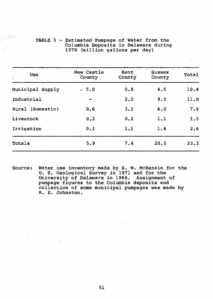
TABLE 5 - Estimated Pumpage of Water from theColumbia Deposits in Delaware during1970 (million gallons per day)

Use New Castle Kent Sussex TotalCounty County County

Municipal Supply .. 5.0 0.9 4.5 10.4

Industrial 2.0 9.0 11.0

Rural (domestic) 0.6 3.2 4.0 7.8

Livestock 0.2 0.2 1.1 1.5

Irrigation 0.1 1.1 1.4 2.6

Totals 5.9 7.4 20.0 33.3

Source: Water use inventory made by S. W. McKenzie for theU. S. Geological Survey in 1971 and for theUniversity of Delaware in 1966. Assignment ofpumpage figures to the Columbia deposits andcollection of some municipal pumpages was made byR. H. Johnston.

51

Pumpage from the Columbia (Pleistocene) deposits inDelaware was 16.1 mgd in 1953, according to Marine andRasmussen (1955, Table 7). Thus, pumpage has more thandoubled in the l7-year interval from 1953 to 1970.

Pumpage for irrigation varies greatly in Delaware fromyear to year depending upon precipitation during the summer.In 1970, a year of average precipitation, pumpage for irri­gation was a modest 2.6 mgd as shown in Table 5. However,in 1966, a very dry year, pumpage for irrigation was con­siderably higher as reported by Sundstrom and Pickett (1968,1969, 1970, and 1971).

Potential Development

General Availability of Water from theColumbia Deposits

The current pumpage from the Columbia deposits (33 mgd)represents only about 4 percent of the natural dischargefrom the aquifer (800 mgd). Therefore, it is apparent thata much greater amount of water can be withdrawn from theaquifer. The question is how much greater can pumpage bewithout producing undesirable effects? The term "safe yield"has been used in the past to describe the amount of waterthat can be withdrawn from an aquifer on an indefinitely longbasis. However, the interpretation of what is "safe yield"is controversial among hydrologists. Probably the mostpractical definition of safe yield has been given by Lohman(1972) as follows: "the amount of water one can withdrawwithout getting into trouble." What constitutes "trouble"in pumping from the Columbia deposits of Delaware? Toanswer this question it is necessary to review briefly thehydrologic effects of withdrawing large amounts of water fromwells.

In what has become a classic paper in hydrology, Theis(1940) has described the essential factors involved in theresponse of an aquifer to pumping from wells. As noted byTheis, all water discharged by wells must be balanced by aloss of water somewhere. Initially, there will be a loss ofwater from storage in the aquifer. Later, as the cone ofdepression expands, recharge must increase ·(if recharge waspreviously rejected), or the natural discharge to streamsmust decrease, in order to balance the loss of water.

Figure 14 shows the manner in which the cone of depres­sion theoretically expands around a well pumping at a con­tinuous rate of 500 gpm from the Columbia deposits. In

52

TRANSMISSIVITY rn : 7000 FT.2/0AY (53,000 GPOI FT.)STORAGE COEFFICIENT (S) : 0.15

a

2

4I I

61~o{

b ,Qi+'

8'

O(!)~O

...lLIlLI 10IL

Z..Z

01 •01 0

0• 14<I:0:0

16

221 I I II&J..J

2

enI&J

~ I2C\I

24 , 10 100 1,000

DISTANCE FROM PUMPED WELL, IN FEET

10,000 100,000

Figure 14. Drawdown around a hypothetical pumped well discharging at 500 gallonsper minute from Columbia deposits of average transmissivity.

preparing Figure 14, the average transmissivity (7,000ft 2/day) and the average (long-term) specific yield (0.15)for the Columbia deposits in central and southern Delawarewere applied to the Theis (1935) equation to compute thedrawdown shown. It is evident from Figure 14 that the coneof depression will extend about 600 feet from the well after1 day of pumping and, theoretically, will extend about 2miles from the well after 1 year of continuous pumping. Asobserved by the writer, the average distance from perennialstreams to the ground-water divide in central and southernDelaware is about 4,000 feet. Therefore, the cone of depres­sion will probably intersect a stream before a year of pump­ing elapses. Initially some water that would naturallydischarge to the stream. will be diverted to the well. Laterwater may percolate through the streambed into the aquiferand be diverted to the well. Although the streams arepartially penetrating, vertical head losses within theColumbia aquifer are usually very small, and the streams canbe treated as fully penetrating when considering their inter­action with well pumpage.

In addition, lowering of the water table may reducedirect evapotranspiration from the aquifer immediatelyadjacent to the stream (where the water table is normallyshallow), and additional water will be diverted to the well.

In some parts of Delaw~re, upward leakage into theColumbia deposits or downward leakage into the Mioceneaquifers is substantial under natural conditions. In theseareas, pumping a well in the Columbia deposits will causeeither an increase in upward leakage or a decrease in down­ward leakage. The term capture has been applied to anydecrease in natural discharge from an aquifer (direct evapo­transpiration, ground-water runoff to streams, or leakage)brought about by pumping (Lohman and others, 1972).

When the amount of the captured water from all sourcesequals the pumping rate of the well, the sy.stem will be inequilibrium and there will be no further expansion of thecone of depression. pumping from additional wells willdisturb the equilibrium and require expansion of the com­posite cones of depression to capture more water. Anothereffect produced by pumping is reduction of the saturatedthickness of the aquifer which, in turn, reduces the trans­missivity. The result of a reduction in transmissivity isthat a deepening of the cone of depression is required tomaintain the same pumping rate.

The relative importance of each of the sources con­tributing water to a pumped well should be considered in

54

assessing the availability of water from the Columbia deposits.Reduction in direct ground-water evapotranspiration (ET) isprobably not an important source of "captured" water movingtoward a pumped well. There is not a great difference betweenthe mean annual base flow (0.86 cfsm) and the mean winter baseflow (1.03 cfsm) of streams draining the aquifer (Table 4).There are several factors ,which could be responsible for thisdifference, one of which is direct ET from the water tablenear streams. Even if it assumed that the entire base flowdifference is due to direct ET and if the unlikely assumptionis made that all this water loss could be captured, therewould not be a substantial contribution to a pumping well.Inducing an appreciable amount of water to move upward fromthe Miocene artesian aquifers, across confining clay beds, istheoretically possible but difficult to achieve in practice.Appreciable upward movement will occur only if there is asubstantial head difference (between the water table in theColumbia deposits and the potentiometric surface in theartesian aquifer) over a large area. As shown in Figure 14,the drawdown around a well pumping from the Columbia depositsis relatively small (less than 10 feet) at distances greaterthan a few hundred feet from the well. In summary, it isprobable that most of the water diverted to a well pumpingfrom the Columbia deposits (after the initial period ofreduction in aquifer storage) is water that would naturallydischarge to streams. Therefore, large long-term withdrawalsof water from the Columbia deposits will probably be balancedby nearly equal reductions in the base flow of streams.

Returning to the question of what is the "safe yield" ofthe aquifer, it is apparent that the "trouble" that must beconsidered is reduction of streamflow. As noted earlier,ground-water runoff constitutes about 72 percent of the totalstreamflow. Therefore, if 100 mgd were continuously with­drawn from the Columbia deposits, the total ground-waterrunoff (800 mgd) would be reduced by 12 percent and the totalstreamflow would be reduced by 9 percent. In practice, then,the "safe yield" of the Columbia deposits is that amount ofreduction in streamflow that is permissible. Of course, ifwater pumped from the aquifer is returned to the drainingstream and not "consumed" or transported out of the basin,there is no stream depletion problem. Surface water is notused for public water supplies in central and southernDelaware. However, uses of surface water include smallwithdrawals for industrial purposes and a small amount forirrigation plus use of the streams for recreational purposesand sewage dilution. The decision as to the amount ofstreamflow depletion permissible really becomes a local basinproblem. Where a small basin is underlain by a highly trans­missive aquifer and the surface water is not used, a largereduction in streamflow might be permissible. On the other

55

hand, if the surface water is used and the aquifer trans­missivity is low, it might be undesirable to reduce stream­flow; the low transmissivity probably would make it costlyand impractical to do so anyway.

Sundstrom and Pickett (1968, 1969, and 1970) estimatedthat 320 mgd of ground water is available from the water­table aquifer in central and southern Delaware. However,note that withdrawal of 320 mgd, if balanced by an equalreduction in ground-water discharge, would result in a30percent decline in total streamflow. On the other hand, ifa large part of the 320 mgd were returned to streams directlyor by way of the Pleistocene deposits, as would be expected,the 30 percent decline in total streamflow would be reducedproportionately. To mi~imize the effect on streamflow,Sundstrom and Pickett (1970) suggested planning ground-waterwithdrawals to capture as much evapotranspiration as possiblein areas of high water table or swamps. However, as notedpreviously, rates of ground-water evapotranspiration appearto be low in most areas, and this method of "capturing" wateris probably not feasible except in swampy areas. Sundstromand Pickett (1970) also suggested using ground-water pumpagefor supplementing the base flow of streams during droughts.This could readily be accomplished by returning a large partof the normal ground-water pumpage directly to streams.

In summary, the amount of possible withdrawal of waterfrom the Columbia deposits in central and southern Delawareis limited to the ground-water runoff to the streams (about800 mgd). However, the desirable or aractical rate of with­drawal is less than this amount depen ing upon: (1) thedesired rate of streamflow in any particular area, and (2)the amount of ground-water pumpage returned to the streamsor the aquifer.

Availability of Large Ground-Water Supplies

The need for large ground-water supplies in central andsouthern Delaware falls into two general categories:

(1) High-capacity wells that can be pumped atrates of 500 gpm or more for relativelyshort periods. Such wells are used byseasonal resorts, particularly duringsummer weekends and for irrigation.

(2) High-capacity wells that can be pumpedcontinuously to supply the year-roundneeds of industries and public watersupplies.

56

In the first case, it is desirable to construct a wellin a thick saturated section of Columbia sand characterizedby high transmissivity. As noted earlier, the avera~e trans­missivity of the Columbia deposits is about 7,000 ft /day(53,000 gpd/ft) and the average saturated thickness is about75 feet. Figure 14 shows the drawdown around a pumping welltapping the Columbia deposits, assuming average transmis­sivity. It is apparent from Figure 14 that wells constructedin such an aquifer can readily yield 500 gpm, with relativelysmall drawdown for short periods of time. Pumped water willcome primarily from storage in the aquifer, which is readilyreplaced during the nonpumping period (the winter-springperiod of ground-water recharge).

Within the areas of high transmissivity shown in Figure 9(T greater than 10,000· ft 2/day), properly constructed wellsshould produce 500 gpm with little drawdown. For shortperiods, 1,000 to 2,000 gpm can be obtained from these wells.Note that 25 wells with reported short-term yields exceeding1,000 gpm are listed in Table 7.

Actually throughout central and southern Delaware, wherethe average saturated thickness of the Columbia deposits is75 feet, properly constructed large-diameter wells shouldproduce 500 gpm or more in most areas. To obtain a yield of500 gpm from such an aquifer, a specific capacity of about10 gpm per foot of drawdown is needed. As shown in Figure 13,almost 90 percent of the large-diameter wells tapping theColumbia deposits in Delaware have specific capacitiesexceeding 10 gpm per foot.

Obtaining high-capacity wells capable of continuouslyyielding 500 gpm or more requires consideration of factorsother than the transmissivity and saturated thickness of theaquifer. This is particularly true if a well field is neededthat will continuously yield several million gallons per day.As noted in the previous section, most water obtained from acontinuously pumped well in the Columbia deposits is (aftera long period) water that would naturally discharge to streams~

An ideal method of obtaining very large supplies of waterfrom the Columbia deposits is to locate wells in highly trans­missive sand and gravel adjacent to a stream characterized byhigh base flow. Such wells may obtain large amounts of waterby diverting water that naturally discharges from the aquiferto the stream, as well as diverting water already in thestream through the streambed into the aquifer. The hydrologicsituation in two areas that meet these requirements will bediscussed here. One if a proven area near Salisbury, Md., andthe other is an undeveloped area near Milton, Del., which wasinvestigated during this study.

57

Channel-fill deposits of Pleistocene age, located betweenSalisbury, Md. and the Delaware-Maryland state line, areideally situated for development of a large water supplyutilizing streambed infiltration. These highly permeablesand and gravel beds attain a maximum thickness of 220 feet(Hansen, 1966) and the transmissivity as determined from a30-day aquifer test is 400,000 gpd per ft (Mack and Thomas,1972). Under natural conditions, the Pleistocene depositsdischarge about 7 cfs (3,100 gpm) into two streams: LittleBurnt Branch and the North Prong Wicomico River. During theaquifer test, one well, near Little Burnt Branch, was pumpedcontinuously at 4,000 gpm. After 30 days of pumping Mack andThomas (1972) concluded that the well was obtaining somewater that had been discharging naturally to the two streamsand some water that was already in the streams. The flow inLittle Burnt Branch declined sharply and had the test con­tinued 3 or 4 more days, the stream would have gone dry.According to Mack and Thomas (1972), at pumping rates lessthan 400 gpm, the pumped water would initially come fromaquifer storage and later would be derived from water intransit to the stream plus some from local recharge. However,when the pumping rate is increased from about 400 gpm to4,000 gpm, water in Little Burnt Branch moves through thestreambed into the aquifer. Note that the Pleistocenechannel aquifer near Salisbury has the highest known trans­missivity on the Delmarva Peninsula. However, it is theclose proximity of the draining streams and the highlypermeable streambed in Little Burnt Branch that make possiblethe large amounts of water available from wells in thisaquifer.

Beaverdam Creek basin near Milton, Del. has hydrologiccharacteristics favorable for the development of a largewater supply by diversion of streamflow. Figure 15 showspertinent hydrologic features in the downstream part of thebasin including water-table contours, ground-water pickupalong the stream, and a brief lithologic log. As shown inthe log, the Columbia deposits contain 132 feet of sand andgravel (110 feet of which is saturated). The transmissivityof the Columbia deposits is about 100,000 gpd per ft basedon a 48-hour aquifer test (see discussion of this test inthe section on aquifer coefficients). Beaverdam Creek ischaracterized by the highest base flow per square mile inDelaware. During 1970, a year of slightly below-averageprecipitation, the average ground-water runoff was 11.8 cfs(7.6 mgd) which is equivalent to 1.65 cfs per square mile,almost twice the average ground-water runoff (0.86 cfsm)listed for other Delaware streams in Table 4. There issubstantial ground-water discharge to the stream in thestretch from Hunter's Mill Pond to the gaging station, asshown by a seepage run made in April, 1969 (Figure 15).

58

N

f

COLUMBIA(PLEISTOCENE)

DEPOSITS

o 1000 2000 FEET

LITHOLOGIC LOGAT WELL Ng55-4(SEE FIGURE I.)

0....,.,...,-,-,-,::::. ::. e._.:.. -0-•e. : "0.:C;.~. "..° 0 °.~ .. '?cp c;~o· o·.0"o· o.0:0 ;'-.0 •

: c..~'0 ••••

::~: CONFINING BED,:,"",.-.:':".:::; MANOKIN AQUIFER

I

/ ~PPROXIMATE BOUNOARY/ OF GROUND-WATER BASIN

_TEA -TABLE CONTOUR(FEET ABOVE MEAN SEA LEVEL)

/

"­"­

"-\.

\.\.

\.\.

\.\.

\

\\ \

)ROUTE 2!59---

I

\;,

' ./;~:SED SITE OF./WELL FIELD SUPPLIED

BY STREAM INFILTRATION

/

(0.76 CFS I M1 2)

/ ­......--./...../'

./

/'!IJSTR[A~ DiSCHARGE MEASUREMENTS MADE ON APRIL 17. 1969 UNDER LOW BASE FLOW CONDITIONS.WATER-TA8LE CONTOURS AFTER BOGGESS, ADAMS AND COSKERY (1964).

Figure 15. aydrologic conditions in part of Beaverdam Cre~k

Basin near Milton, Del.59

Similar quantities of ground-water inflow were computedusing airborne radiometric temperature measurements, asreported by Hollyday (1970).

The very high base flow in Beaverdam Creek (1.65 cfsm)cannot be accounted for by discharge from the Columbiadeposits alone. The test drilling disclosed that permeablesands of the Miocene Manokin aquifer underlie the Columbiadeposits with only a thin (IS-ft) confining bed (silt)separating the two aquifers. It seems probable that upwardleakage from the Manokin contributes to the exceptionallyhigh base flow of Beaverdam Creek (Johnston, 1971).

Seve~al factors affect the yield of a well field suppliedby water diverted fromoa stream. These factors have beensummarized by Rorabaugh (1963). In Beaverdam Creek basin,the ultimate yield of a well field will depend primarily on:

(1) the ability of the streambed to transmitwater (vertical hydraulic conductivity ofthe sand and silt constituting thestreambed),

(2) the transmissivity of the aquifer,

(3) the average base flow of the stream, and

(4) the ability of wells to capture groundwater en route to the stream.

Figure 15 indicates that the greatest ground-waterpickup occurs between Hunter's Millpond and Route No. 260.Wells in this area would be expected to have the greatestchance of capturing ground water before it discharges to thestream. On the other hand, a well field located downstreamnear the gaging station would be in a position to divert theentire flow of the stream, if necessary.

The most important factor in selecting the location ofwells to be supplied by streambed infiltration may be thehydraulic conductivity of the silty layer on the streambed.A line of shallow observation wells constructed at rightangles to a stream is probably the best approach to eval­uating the hydraulic nature of the silty layer. If thewater table profile has a gradual slope and is continuouswith the stream surface, the silty layer is probably not aneffective barrier. If the water table is above or below thestream surface immediately adjacent to the stream, the siltylayer is an effective seal.

A line of piezometer tubes constructed at right anglesto the stream at the Beaverdam Creek gaging station indicated

60

a steeply sloping water table. At a tube 20 feet from thestream, the water table is 0.5 to 1.0 foot above the stream.In addition, small seeps occur in the stream bank a few feetabove the stream surface. All these data suggest that thesilt bed is probably an effective barrier near the gagingstation.

A suggested location for a well field to be supplied bystreambed infiltration iS'shown in Figure 15. The site isin the downstream part of the reach of greatest ground-waterpickup and is within a quarter of a mile of the aquifer testsite where high transmissivity has been confirmed. Theground-water runoff of the stream at the proposed well fieldis about 80 percent of that measured at the gage. Thus,ground-water runoff during 1970 would have been 9.4 cfs or6.1 mgd. The 6 mgd figure gives an approximate indicationof the amount of water that could be pumped continuously atthe proposed well field. Lowering of the water table mightinduce additional water to move up from the Manokin aquifer;however, the amount of such additional water cannot beestimated with present information. It is unlikely thatadditional water can be obtained by reduction of evapotran­spiration as the water table is lowered. The water table is20 feet below land surface a short distance from the streamand ground-water evapotranspiration is probably very smallat present.

The fact that the part of Beaverdam Creek basin shownin Figure 15 is less than 10 miles from Lewes and RehobothBeach (see Figure 1) suggests that the area could be a usefulfuture source of water for the fast-developing seashore area.At present, combined pumpage of ground water along theDelaware Atlantic seashore (Lewes, Rehoboth Beach, BethanyBeach, etc.) is about 4 mgd (Miller, 1971). This water issupplied by a large number of wells, and some salt-watercontamination has occurred in shallow wells near the beaches.In contrast, three or four properly constructed large-diameterwells located in the Beaverdam Creek basin should readilyyield 4 mgd, and the location about 7 miles inland wouldminimize the possibility of salt-water encroachment.

The advantages of a well field supplied by streambedinfiltration over a well field supplied only from aquiferstorage may be summarized as follows:

(1) By utilizing induced infiltration, arelatively large supply of water can beobtained from a few wells at one site.In contrast, many wells, more widelyspaced, would be needed to supply thesame quantity of water from the Columbiadeposits if the wells were not near astream.

61

(2) Objectionable characteristics of surfacewater, such as turbidity and inconsistenttemperature, are usually removed orattenuated during percolation through theaquifer.

The major disadvantage of an induced-infiltration supply isthat streamflow is reduced and the stream can go dry undermaximum pumpage.

Wells suppled by river infiltration have been developedin many areas, including the Ohio, Mississippi, and MohawkRiver valleys. In some of those areas, very large watersupplies have been developed by horizontal-type collectorwells, which are effective in increasing rates of infiltra­tion through the streambed. However, large infiltrationsupplies have also been-obtained by conventional verticalwells in Louisville, Ky. and Schenectady, N.Y.

Wells obtaining water by streamflow infiltration arenot common in Delaware at present. In the Seaford area,where about 4 mgd is withdrawn from the Columbia deposits, alarge part of the pumpage is probably ground water thatnaturally discharges into the Nanticoke River and some ofthe water may be obtained from streambed infiltration. AtSmyrna, Del., a supply well at the Delaware State Hospitaland one of the town supply wells tap a permeable sandaquifer within 200 feet of Lake Como. At high sustainedpumping rates, those wells may obtain water by infiltrationfrom the lake.

The potential for developing very large infiltrationsupplies in the Delaware Coastal Plain is limited becausethe area is drained by many small streams. The two largeststreams, the Nanticoke River and Marshyhope Creek, whosedrainage areas are 75 and 44 square miles, respectively,have sufficient base flow to support large supplies derivedfrom stream.infiltration. The Columbia deposits have anaverage thickness of about 50 feet in the Marshyhope basin.However, almost nothing is known of the aquifer transmis­sivity in this basin. In the Nanticoke basin, the range oftransmissivity is wide (6,000 to 80,000 gpd per ft), and thepossibility exists that a site suitable for a large infiltra­tion supply can be found.

A few smaller basins probably have the potential fordeveloping infiltration supplies. In each case, a prelim­inary study, such as was made in the Beaverdam Creek basin,would be needed to assess the area as a possible infiltrationsupply. The study ideally would include test drilling,seepage runs along the stream, and a preliminary aquifer test.

62

QUALITY OF WATER AND GROUND-WATER CONTAMINATION

Water from the Columbia deposits is generally "soft,"slightly acidic, and characterized by low dissolved-solidcontent. High iron content and low pH are the only naturalcharacteristics of the water that commonly require treatment.However, local problems of ground-water contamination haveoccurred in recent years due to salt-water intrusion in afew coastal areas, waste disposal, and accidental spills.

Table 6 lists the major chemical constituents in groundwater from the Columbia deposits. The table is based onchemical analyses made by the U. S. Geological Survey onsamples from 19 wells. Several additional analyses were notincluded because of known or suspected contamination by salt­water encroachment or waste disposal. Table 6 is, therefore,an attempt to show the "natural" chemical quality of theground water. The principal constituents, as shown in Table6, are calcium, sodium potassium, silica, bicarbonate, sulfate,chloride, and nitrate. Hardness (both the calcium magnesiumand noncarbonate varieties) is generally low and treatment isusually not necessary.

High iron content is a common water-quality problem inthe Columbia deposits. About one-third of the wells listedin Table 6 produced water containing more than 0.3 mg/l --the maximum recommended for drinking water by the U. S. PublicHealth Service (1962). Such water will cause reddish-brownstaining and produce iron scale which may clog pipes or wellscreens. However, iron may be removed by several methodsincluding aeration and filtration and treatment with lime orpolyphosphates.

The occurrence of iron in the Columbia deposits issporadic. The highest reported iron concentrations occur atRehoboth Beach and Selbyville (Rasmussen and others, 1960),and the lowest occur northwest of Seaford (Woodruff, 1970).The iron-rich water at Selbyville is the subject of a currentgeochemical investigation by John C. Miller of the DGS.

The position of the Columbia deposits near land surfacemakes the aquifer particularly susceptible to contaminationby leachates from landfills and dumps, effluent from septictanks, and accidental spills. In a recent survey of ground­water contamination in the northeastern states, 9 of 12 casescited for Delaware involved the Columbia (Pleistocene)deposits. Contamination of the ground water by effluent fromseptic tanks or cesspools reportedly has occurred at Dover,St. Georges, and Laurel. In one of those areas, located justsouth of Dover, Miller (1972) determined that the water in 6of 13 domestic wells sampled contained nitrate concentrations

63

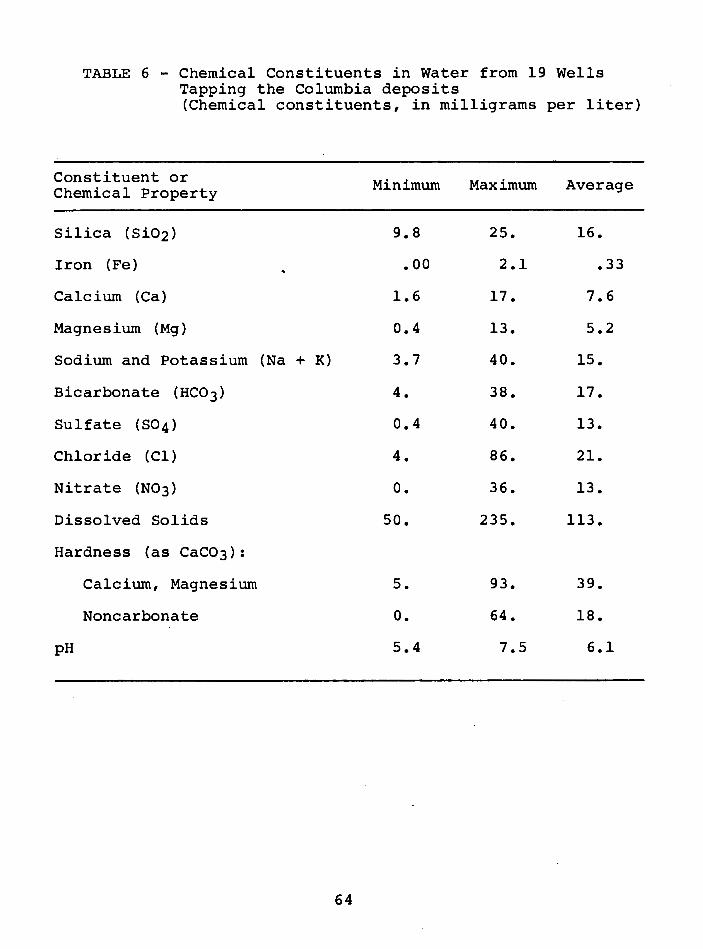
TABLE 6 - Chemical Constituents in Water from 19 WellsTapping the Columbia deposits(Chemical constituents, in milligrams per liter)

Constituent or Minimum Maximum AverageChemical Property

Silica (Si02) 9.8 25. 16.

Iron (Fe) .00 2.1 .33

Calcium (ca) 1.6 17. 7.6

Magnesium (Mg) 0.4 13. 5.2

Sodium and Potassium (Na + K) 3.7 40. 15.

Bicarbonate (HC03) 4. 38. 17.

Sulfate (S04 ) 0.4 40. 13.

Chloride (Cl) 4. 86. 21.

Nitrate (N03) o. 36. 13.

Dissolved Solids 50. 235. 113.

Hardness (as CaC03):

Calcium, Magnesium 5. 93. 39.

Noncarbonate o. 64. 18.

pH 5.4 7.5 6.1

64

exceeding the maximum level of 45 mg/l recommended fordrinking water by the U. S. Public Health Service (1962).Other reported cases of ground-water contamination have beencaused by seepage of salty water from a dredging spoil areaalong the Chesapeake and Delaware Canal, seepage of saltywater from an uncovered salt pile near Christiana, andleakage from gasoline storage tanks near Laurel.

Salt-water contamination of the Columbia deposits is alocal, but not as yet serious, problem in the coastal areasof Delaware. During the 1940's, salty ground water appearedin wells used by the towns of Lewes, New Castle, andRehoboth Beach. For Lewes and Rehoboth Beach, it was nec­essary to drill new wells farther inland from the beach.

The salt-water problem was not investigated in thecurrent hydrologic appraisal of the Columbia deposits.However, any projected large withdrawals of water from thisaquifer in the coastal zone ideally would include a localsite investigation of salt-water encroachment. The salt­water problem has been reviewed in general terms by Sundstromand Pickett (1970) and a detailed discussion of salt-waterencroachment at Lewes is given by Rasmussen and others (1960).

APPLICATION OF FINDINGS

The findings of this report should be helpful in thedevelopment of large ground-water supplies in central andsouthern Delaware. The important factors to be kept in mindwhen developing water supplies from the Columbia (Pleistocene)deposits are as follows:

(1) Water in the Columbia deposits and much ofthe water in streams is, in effect, "onewater." This conclusion is based on thefact that discharge of ground water fromthe Columbia deposits supplies about three­quarters of the streamflow. In contrast,overland runoff supplies only one-quarterof the streamflow. Therefore, if largeamounts of ground water are pumped, it mustbe anticipated that declines in streamflowwill occur (unless the pumped ground wateris returned to streams or the ,aquifer).Conversely, if water is to be withdrawnfrom a stream, ground water cannot also bepumped on a large scale.

65

(2) Large supplies of ground water (morethan 1 mgd) can be most easily andeconomically obtained by constructingwells in areas of high transmissivity(shown in Figure 9) adjacent to streamscharacterized by high base flow. Wellsat such sites may obtain large amounts ofwater by diverting ground water thatnaturally discharges to a stream and,also, by diverting water already in thestream to move through the streambed intothe aquifer.

(3) The 800 mgd of water that discharges fromthe Columbia deposits is not the "safeyield" of the· aquifer. TJi'I'S water providesthe fair-weather (base flow) of streams incentral and southern Delaware as well asground-water pumpage from the aquifer.

The discussion of Beaverdam Creek basin near Miltonprovides an example of how to identify an area of highground-water potential. A gaging station provided the nec­essary streamflow record from which it was determined thatthe stream had very high base flow. High transmissivity wassuspected based on nearby well logs, geologic data, and base­flow data. Exploratory drilling and a pumping test confirmedthe existence of a thick section of Columbia deposits andhigh transmissivity. The maps of saturated thickness andtransmissivity (Figures 3 and 9) presented in the report areintended to help those interested in identifying similarareas in the future.

Note that high transmissivity alone will not insure thepermanence of a large ground-water supply. High T meansthat, initially, well yields and specific capacity will behigh. However, unless the draining stream or streams arecharacterized by high base flow, the wells are dependentprimarily on aquifer storage, and as pumping proceeds,yields may decline.

An area southwest of Houston (Figure 1) is a case inpoint. At this site, the Columbia deposits have the highesttransmissivity (22,000 ft 2/day or 165,000 gpd/ft) known todate in Delaware. The site is very near the divide betweenthe drainage areas of the Chesapeake and Delaware Bays. Thenearby stream, Beaverdam Branch, drains less than 3 squaremiles and the total base flow is small. Within this smallbasin a ground-water supply of about 1.5 mgd can be effi­ciently and economically developed from one or two high­capacity wells. However, despite impressive yields from

66

one or two wells, this small basin will never provide a verylarge supply of ground water.

In addition to providing suggestions for the futuredevelopment of large ground-water supplies from the Columbiadeposits, this report is intended to supply technical datafor more sophisticated hydrologic studies. Ideally suchstudies would take the form of digital or electric analogmodels of the stream-aquif~r system. These model studiescan provide an understanding of the workings of the systemand can also be used as water-management tools.

67

TABLE 7 - Yield and specific capacity of lat ge-diameter wel ls tapping the

Columbia (Pleistocene) deposists and estimated transmissivity of the aquifer

Screened Yie ld Specific Estimated transmissivityWell -Ow ner Depth Diameter interval (ga llons capac ity

number (feet) (inches) (feet) per minute) (gpm/ft) gal /day/ft T ft2 /da y

Cd 42-13 Artesian Water Co. 73 17 49 73 570 38 60,000 8,000

Cd 43 -6 Atlas Chemical Ind ust r ies, Inc. 71 26 52 67 600 27 40,000 5,300

Cd 51 -1 Artesian Water Co. 47 17 24 - 47 350 10 18,000 2,400

Db 31 -19 E. I. du Po nt Co . 65 10 53 - 65 100 8 14,000 1,900

Db 31-35 E. I. du Pont Co . 80 8 70 - 80 500 11 9,000 1,200

Dc 53 -5 Getty Oi l Co. 90 8 70 - 90 525 48 72,000 9,600

Eb 55-4 Baker Brothers 40 17 16 - 40 600 19 30,000 4,000

Eb 55 -5 Warren Baker 45 17 17 - 45 450 24 36,000 4,800

Ec 41-7 Fred Haas 93 17 29 - 89 220 4 6,000 800

Fb 23-6 Fred Wicks 71 8 30 - 70 100 8 .3 12 ,000 1,600

Fb 34-16 Un iversity of De laware 74 8 54 - 74 110 3.5 33,000 4,500

Fb 51-4 George & Sam Brooks 44 17 24 - 44 520 19 29,000 4,000

Fb 51-5 George & Sam Bro o ks 44 17 16 - 44 620 20 30,000 4,000

Fb 51-6 Norman & Sam Bro o ks 54 17 300 12 19,000 2,500

Fb 53-7 Chris Wicks 80 17 21 - 80 580 9 14,000 1,900

Ga 15-4 Gerald Zeh 63 17 30 - 60 1,120 51 76 ,000 10,000

Hc 32-5 City Products Corp. 56 10 43 - 56 325 20 36,000 4,800

68

TABLE 7 - (continued)

Screened Yield Specific Estimated transmissivityWell _ Owner Depth Diameter interval (gallons capacity

number (feet) (inches) (feet) per minute) (gpmjft) galjdayjft I ft 2 jday

Hc 32-12 W. L. Wheatley, Inc. 77 12 780 14 25,000 3,300

Hc 34-3 City of Smyrna 100 10 70 - 100 550 30 54,000 7,200

Hc 34-22 City of Smyrna 96 12 55 - 85 1,100 54 120,000 16,000

Hc 43-3 George Wicks 115 10 1,020 82 150,000 20,000

Hc 44-3 George Wicks 133 12 75 - 132 1,050 88 160,000 21,000

Hc 55-1 Walter Gibe 120 10 90 - 120 1,000 52 93,000 12,000

Ie 32-4 Frank Johnson 48 12 350 ? 5 9,000 1,200

Id 24-4 Philip Cartanza 157 17 25 - 157 1,050 20 30,000 4,000

Ie 31-1 Joseph Zimmerman 94 17 16 - 94 940 19 28,000 3,700

Ie 43-2 Philip Cartanza 106 17 16 - 103 1,400 50 75,000 10,000

Ie 53-2 Alfred Bilbrough 114 17 21 - 113 700 54 82,000 11,000

Ie 53-3 Alfred Bilbrough 72 17 36 - 72 750 17 25,000 3,300

Ie 53-4 Alfred Bilbrough 70 17 13 - 69 720 21 32,000 4,200

Jc 34-1 Joseph Wild 97 17 20 - 96 900 17 25,000 3,300

Jd 12-2 Eugene Gagan 104 17 40 - 96 1,300 22 33,000 4,400

Jd21-2 Papen Farms 96 17 40 96 760 17 23,000 3,100

Jd41-1 Libby, McNeil, & Libby, Inc . 125 10 87 - 109 400 9 15,000 2,000

69

TABLE 7 - (conti ll ued'

Screen ed Yi eld Specif ic Estim ated transmissivi ty\\' l'i I 0 v, ncr Depth Diameter interval (gaII()ns capacity

IlU mb er (feet) (inches) (feet) per minute) (gpm,lft ) gdlj ddy j ft f t 2 j day

[d 54- 1 Joseph [ackewi ez 118 17 26 · 118 1,260 21 38 ,000 5,100

Je 12-2 Jacob Zimmerm an 72 10 600 16 24 ,000 3,200

Je 13-1 A lfred Bilbro ugh 70 17 18 66 780 21 31,000 4,200

Kd 24-2 Joseph Kowalski 134 13 38 134 1,050 21 31,000 4,200

Ke 12-2 Kenneth Bergold 146 17 30 - 74 ; 1,600 44 67,000 9,000122 - 146

Ld 33-1 Walter Wink ler 64 17 20 · 56 ; 1,400 39 60,000 8,00060 - 64

Le 22-2 Charles West 73 8 13 73 400 11 17,000 2,300

l.e 23-3 Char les West 74 13 22 · 74 380 9 14,000 1,900

Le 51-2 Flo yd Blessing 105 17 1,200 64 96 ,000 13,000

Md 15-8 Libb y , McNeil , & L ibby , Inc. 67 10 41 67 280 + 22 40,000 5,300

Md 24-3 U. S. Geological Survey - DelawareGeological Survey 80 8 70 - 80 300 + 10 165,000 22 ,000

Md 54-2 John Ann et 82 17 30 - 82 1,180 53 80 ,000 11 ,000

\\e 24-5 Cit y of Mi lfor d 80 8 400 18 26 ,000 3,500

,\ 1e 24-6 Cit y of Milf ord 69 12 39 - 59 520 29 42 ,000 5,600

\1<: 33-3 Donald Calhoun 74 17 38 70 700 30 45 ,000 6,000

Me 54-5 Delmarva Nursery 90 8 58 90 500 20 30,000 + 4,000 +

iO

TABLE 7 - (cont inur d )

Screened Yield Specific Estimated tr ansmi ssivit yWell Owner Depth Diamet er int erval (gallo ns capa city

number (feet ) (inches) (fee t ] per minute] (gpm jft ) gal jdayjft ft2 jday

Mf 11-6 Cit y of Milford 67 220 25 44 ,000 5,900

Mf 21 -1 Diamond State Nur series 63 8 18 0 15 27,000 3,600

Mf 22-4 Brown Thawley 131 17 44 - 106 1,400 80 120,000 16,000

Mg 42-13 Draper Foods, Inc . 89 8 69 - 89 150 + 35 50,000 6 ,700

Nc 25-19 Bramble Canning Co . 84 1,300 24 36,000 4 ,800

Nc 53-3 O. A. Newton & Sons 100 12 1,080 22 33,000 4,400

Nd 33 -1 J. Howard Lyons 92 17 1,200 30 45,000 6,000

Ng 12 -1 Carlton Clifton 61 6 300 17 31,000 4,100

Ng 31-1 Willard Workman 122 17 900 74 110,000 "' 5 ,000

Ng 41-2 Willard Workman 112 17 1,080 32 48,000 6,400

Ng 42 -1 Town of Milton 68 6 200 31 56,000 + 7,500 +

Ng 42-15 Draper Canning Co . 13 1,300 65 100,000 13 ,000

Ng 42-16 Draper Canning Co. 84 13 1,020 49 73,000 10,000

Ng 55-4 U. S. Geological Survey - DelawareGcological Survey 70 8 60 - 70 200 + 7 104,000 14 ,000

Ni 31-3 Lewes Dairy 60 8 100 + 14 25,000 3,300

71

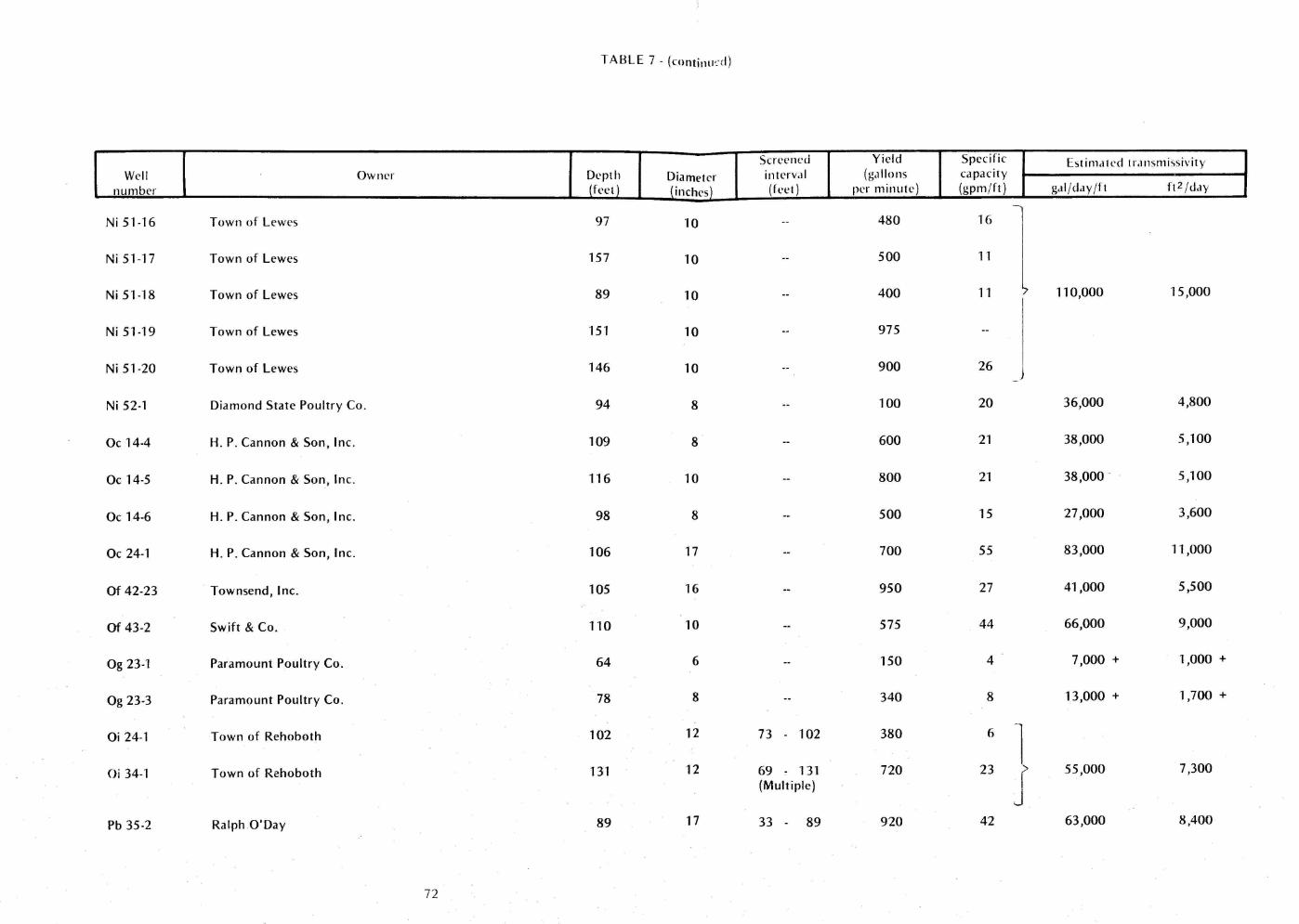
TABLE 7 - (continu'_'d )

Screened Yield Specific Estimated transmissivityWell Owner Depth Diameter interval (gallons capacity

number (feet) (inches) (feet) per minute) (gprn /ft ) gal/day /ft ft 2 /day

Ni 51 -16 Town of Lewes 97 10 480 16 lNi51 -17 Town of Lewes 157 10 500 11I

Ni 51 -18 Town of Lewes 89 10 400 11 l 110,000 15 ,000

Ni 51-19 Town of Lewes 151 10 975

Ni 51-20 Town of Lewes 146 10 900 26

Ni 52-1 Diamond State Poultry Co, 94 8 100 20 36,000 4,800

Oc 14-4 H. P. Cannon & Son, Inc. 109 8 600 21 38,000 5 ,100

Oc 14-5 H. P. Cannon & Son, Inc . 116 10 800 21 38,000 . 5,100

Oc 14-6 H. P. Cannon & Son, Inc . 98 8 500 15 27 ,000 3,600

Oc 24-1 H. P. Cannon & Son, Inc . 106 17 700 55 83 ,000 11,000

Of 42-23 Townsend, Inc. 105 16 950 27 41,000 5,500

Of 43-2 Swift & Co. 110 10 575 44 66 ,000 9,000

Og 23 -1 Paramount Poultry Co. 64 6 150 4 7,000 + 1,000 +

Og 23-3 Paramount Poultry Co. 78 8 340 8 13 ,000 + 1,700 +

Oi 24 -1 Town of Rehoboth 102 12 73 - 102 380 6 -112Oi 34-1 Town of Rehoboth 131 69 - 13 1 720 23 > 55 ,000 7,300

(Multiple) JPb 35-2 Ralph O'Day 89 17 33 - 89 920 42 63 ,000 8,400

72

T ABL E 7 - (c o rn inued]

Ser et.'n cd Yie ld Sp ecifi c [ .,Iim.lll'd tr.l/l smi ssivil\Well Ow ncr Depth Diameter int orva l Ig.d lo ns ca p.rcit ,:

number i fl'c t ) (inches j (f eel I pel min ute ) (gplll /ft ) g,d 'd.!y,!"t t t 2 id ,I\ ', ,

Pc 23-3 Cit y of Seaford 95 10 800 28 50,000 (" ,DO

Pc 33 -5 E. I. du Po nt Co . 98 10 540 12 21,000 2,800

Pc 33 -9 E. I. du Po nt Co . 83 10 640 24 43,000 5 ,700

Pc 33-10 E. I. du Pont Co . 78 10 600 24 43,000 5 ,700

Pc 33- 11 E. I. du Po nt Co. 101 10 620 13 23,000 3,000

Pc 44 -4 Ra lph Given s 109 17 65 - 109 300 + 40 60,000 8 ,000

Pc 54-1 Fred O'Neal 100 17 16 . 100 900 65 100,000 13 ,000

Pd 53-1 Emory Sp icer 164 17 44 - 160 950 38 57 ,000 7,600

Pf 23 -2 H. Kruger, Inc. 180 17 40 - 180 1,200 29 51,000 6,800

Pg 53-8 Town of Millsboro 83 8 250 9 14 ,000 1,900

Pg 53 -9 Town of Millsboro 84 8 180 7 11,000 1,500

Pg 54-1 Millsboro Poultry Co . 105 8 400 12.5 19,000 2,500

Qb 44-5 Howard Rider 111 17 1,070 40 60,000 8 ,000

Qc 14-5 Col eman Wheat ley 98 17 830 49 74,000 10,000

Qc 14-6 Col eman Wheatley 90 17 550 32 48 ,000 6,400

Qc 24-6 Emory Spicer 121 17 1,400 107 160 ,000 2 1,000

Qc 34-1 Pa ul Spear 86 17 78 - 86 1,300 36 54,000 7 ,200

Qh 5 1-7 Town of Frankford 100 8 80 - 100 100 + 22 .5 36,000 4 ,XOO

7 '), J

TABLE 7 - (continued)

Screened Yield Specific Est imat ed t ransmissivityWell . Owner Depth Diameter interval (gallon s capac ity

number (feet) (inches) (feet) per minu te) (gprn /ft ] gal/daY/f t ft2 /da y

Qh 51-10

Qh 51-1 4

Rd 31-11

Rh 32-9

Delmarva Poultry Co.

Town of Frankford

Town of Delmar

Town of Selbyville

74

105

101

139

125

8

8

8

8

80 - 101

105 - 125

240

350 +

300

24

40

18.4

9

38 ,000

64 ,000

33 ,000 ?

16 ,000

5 ,100

8,500

4 ,400

2,100

REFERENCES

Back, William, 1966, Hydrochemical facies and ground-waterflow patterns in northern part of the Atlantic CoastalPlain: U. S. Geol. Survey Prof. Paper 498-A.

Boulton, N. S., 1963, Analysis of data from non-equilibriumpumping tests allowing for delayed yield from storage:Inst. Civil EngineersProc. (London), v. 26, p. 469-482.

Boggess, D. H., Adams, J. K., and Coskery, O. J., 1964,Water-table, surface-drainage, and engineering soilsmap of the Milton quadrangle, Delaware: U. S. Geol.Survey Hydrol. Inv. Atlas HA-102, scale 1:24,000.

Ferris, J. G., and others, 1962, Theory of aquifer tests:U. S. Geol. Survey Water-Supply Paper l536-E, p. 69-174.

Hansen, H. J., 1966, Pleistocene stratigraphy of the Salis­bury area, Maryland: Maryland Geol. Survey Rept. ofInv. No.2, 56 p.

Hollyday, E. F., 1970, Use of infrared radiometry in measur­ing ground-water inflow to streams, Delmarva Peninsula,Maryland and Delaware, in Hydrology and oceanography,second annual earth resources aircraft program statusreview, v. 3: Natl. Aeronautics and Space Adm. MannedSpacecraft Center, Houston, Tex., p. 44-1 to 44-14.

Jacob, C. E., 1943, Correlation of ground-water levels andprecipitation in Long Island, New York: Am. Geophys.Union Trans., v. 24, pt. 2, p. 564-573.

Johnston, R. H., 1971, Base flow as an indicator of aquifercharacteristics in the Coastal Plain of Delaware: U.S. Geol. Survey Prof. Paper 750-D, p. D2l2-D2l5.

Jordan, R. R., 1962, Stratigraphy of the sedimentary rocksof Delaware: Delaware Geol. Survey Bull. 9, 51 p.

, 1964, Columbia (Pleistocene) sediments of Delaware:--~Delaware Geol. Survey Bull. 12, 69 p.

, 1967, Atlantic Coastal Plain Geol. Assoc. 8th Ann.----F=ield Conf. Guidebook, 21 p.

Lohman, S. W., 1972, Ground-water hydraulics: U. S. Geol.Survey Prof. Paper 708, 70 p.

Lohman, S. W., and others, 1972, Definitions of selectedground-water terms -- revisions and conceptual refine­ments: U. S. Geol. Survey Water-Supply Paper 1988.

75

Mack, F. K., and Thomas, W.O., Jr., 1972,channel-fill deposits near Salisbury,determined by a 30-day pumping test:Survey Bull. 31, pt. 1.

Hydrology ofMaryland asMaryland Geol.

Marine, I. W., and Rasmussen, W. C., 1955, Preliminary reporton the geology and ground-water resources of Delaware:Delaware Geol. Survey Bull. 4, 336 p.

Mather, J. R., 1969, Factors of the climatic water balanceover the Delmarva Peninsula: C. W. ThornthwaiteAssociates Pubs. in Climatology, v. XXII, no. 3, 129 p.

Miller, J. C., 1971, Ground-water geology of the DelawareAtlantic seashore: Delaware Geol. Survey Rept. of Inv.No. 17, 33 p. •

, 1972, Nitrate contamination of the water-table---aquifer in Delaware: Delaware Geol. Survey Rept. ofInv. No. 20, 36 p.

Otten, E. G., 1970, Geologic and hydrologic factors bearingon subsurface storage of liquid wastes in Maryland:Maryland Geol. Survey Rept. of Inv. No. 14, 39 p.

Rasmussen, W. C., and others, 1957, The water resources ofnorthern Delaware: Delaware Geol. Survey Bull. 6, 223 p.

, 1960, Water resources of Sussex County, Delaware:----~Delaware Geol. Survey Bull. 8, 228 p.

Rasmussen, W. C., and Andreasen, G. E., 1959, Hydrologicbudget of the Beaverdam Creek basin Maryland: U. S.Geol. Survey Water-Supply Paper 1472, 106 p.

Rima, D. R., and others, 1964, Ground-water resources ofsouthern New Castle County, Delaware: U. S. Geol.Survey Water-Supply Paper 1756, 54 p.

Riggs, H. C., 1963, The base-flow recession curve as anindicator of ground water: Internat. Assoc. Sci.Hydrology Pub. 63, p. 352-363.

Rorabaugh, M. I., 1960, Use of water levels· in estimatingaquifer constants in a finite aquifer: Internat. Assoc.Sci. Hydrology Pub. 52, p. 314-323.

, 1963, Streambed percolation in development of water----~supplies in: U. S. Geol. Survey Water-Supply Paper

l544-H, p-.H47-H62.

76

Rorabaugh, M. I., and others, 1966, Exploration of methodsrelating ground water to surface water, Columbia Riverbasin -- first phase: U. S. Geol. Survey open-filerept., 124 p.

Spoljaric, Nenad, 1967, Pleistocene channels of New CastleCounty, Delaware: Delaware Geol. Survey Rept. of Inv.No. 10, 15 p.

, 1971, Origin of colors and ironstone bands in the-----=Columbia Formation, Middletown-Odessa area, Delaware:

Southeastern Geology, v. 12, no. 4, p. 253-266.

Spoljaric, Nenad, and Woodruff, K. D., 1970, Geology,hydrology, and geophysics of Columbia sediments in theMiddletown-Odessa area, Delaware: Delaware Geol. SurveyBull. 13, 156 p. •

Stallman, R. W., 1965, Effects of water-table conditions onwater-level changes near pumping wells: Water ResourcesResearch, v. 1, no. 2, p. 295-312.

, 1971, Aquifer-test design, observation, and data-----a-nalysis: U. S. Geol. Survey Techniques of Water­

Resources Inv., book 3, chap. Bl, 26 p.

Stallman, R. W., and Papadopulos, I. S., 1966, Measurement ofhydraulic diffusivity of wedge-shaped aquifers drainedby streams: U. S. Geol. Survey Prof. Paper 514, 50 p.

Sundstrom, R. W., and Pickett, T. E., 1968, The availabilityof ground water in Kent County, Delaware, with specialreference to the Dover area: Univ. of Delaware WaterResources Center rept., 123 p.

, 1969, The availability of ground water in eastern-----=Sussex County, Delaware: Univ. of Delaware Water

Resources Center rept., 136 p.

____-=, 1970, The availability of ground water in westernSussex County, Delaware: Univ. of Delaware WaterResources Center rept., 118 p.

____-=, 1971, The availability of ground water in New CastleCounty, Delaware: Univ. of Delaware Water ResourcesCenter rept., 156 p.

Theis, C. V., 1935, The relation between the lowering of thepiezometric surface and the rate and duration of dis­charge of a well using ground-water storage: Am.Geophys. Union Trans., v. 16, p. 519-524.

77

Theis, C. V., 1940, The source of water derived from wells:Civil Eng., v. 10, no. 5, p. 277-280.

____~' 1963, Estimating the transmissibility of a water­table aquifer from the specific capacity of a well, inBentall, Ray, compiler, Methods of determining permea­bility, transmissibility, and drawdown: U. S. Geol.Survey Water-Supply Paper l536-I, p. 332-336.

U. S. Geological Survey, Surface Water Records, pt. 1 ofWater Resources Data for Maryland and Delaware:Published yearly from 1961 to 1970.

U. S~ Public Health Service, 1962, Drinking water standards,1962: U. S. Public Health Service Pub. No. 956, 61 p.

Weeks, E. P., 1969, Determining the ratio of horizontal tovertical permeability by aquifer-test analysis: WaterResources Research, v. 5, no. 1, p. 196-214.

Weigle, J. M., 1972, Exploration and mapping of Salisburypaleochannel, Wicomico County, Maryland: MarylandGeol. Survey Bull. 31, pt. 2.

Woodruff, K. D., 1969, The occurrence of saline ground waterin Delaware aquifers: Delaware Geol. Survey Rept. ofInv. No. 13, 45 p.

, 1970, General ground-water quality of fresh-water----~aquifers in Delaware: Delaware Geol. Survey Rept. of

Inv. No. 15, 22 p.

78