Biostatistics

Lecture 17 6/15 & 6/16/2015

Chapter 17 – Correlation & Regression

• Correlation (Pearson’s correlation coefficient)

• Linear Regression• Multiple Regression

Introduction

• To determine whether there is an association between two variables (one independent and one dependent)

• If so, what is the association?• Can we use it to predict the weight of a male

bear given his body length?

Lengths and Weights of Male Bearsx Length

53.0 67.5 72.0 72.0 73.5 68.5 73.0 37.0

y Weight

80 344 416 348 262 360 332 34

Correlation

• A “correlation” can help determining whether there is a “statistically significant” association between two variables.

• A scatter plot can help visually assessing whether the paired data (x, y) might be correlated.

• Such correlation could be “linear” or in other nonlinear forms (such as exponential, etc.)

Linear correlation

• The linear correlation coefficient r measures the strength of the linear association between the paired x- and y-quantitative values in a sample.

• It is sometimes called Pearson product moment correlation coefficient.

• r ranges between -1 and 1.

Basic requirements before computing r

1. paired data (x, y) are randomly sampled.

2. visual scatter plot be approximately a straight line.

3. outliners be firstly removed

Example 1

Given the following 4 paired data, compute the correlation coefficient r.

x 1 1 3 5

y 2 8 6 4

• It looks like a low negative correlation.

• r = -0.1348

>> x=[1 1 3 5];y=[2 8 6 4];n=4;>> r=(n*sum(x.*y)-sum(x)*sum(y))/sqrt((n*sum(x.*x)-sum(x)^2)*(n*sum(y.*y)-sum(y)^2))

r = -0.1348

>>

Interpreting r

• r is between -1 (perfect negative correlation) and +1 (perfect positive correlation).

• r = 0 means no correlation.• Then what defines a “strong” correlation?• The absolute value of r should be no less

than a critical value?• Is r a random variable having its own

probability density function?

Hypothesis testing for r

• H0: no significant linear correlation

• Test statistic:• This is a 2-tailed t test• DF = n-2• = 0.05 (usually)• p-value can be computed based on

computed t on a t distribution of specific DF.

• Reject if p <= 0.05.

2

1 2

n

r

rt

Back to example 1

• A critical t value that cuts 0.025 off the left tail of tDF=2 is “tinv(0.025, 2) = -4.3027”.

• The t-statistic computed based on previously computed r = -0.1348 now becomes -0.1925.

• -0.1925 is not as extreme or more extreme than -4.3027. We thus do not reject the null hypothesis of no significant linear correlation.

• P-value = 2*tcdf(-0.1925,2)=0.8652, much greater than =0.05.

>> x=[1 1 3 5];y=[2 8 6 4];>> n=4;>> r=(n*sum(x.*y)-sum(x)*sum(y))/sqrt((n*sum(x.*x)-sum(x)^2)*(n*sum(y.*y)-sum(y)^2))

r = -0.1348

>> t=r/sqrt((1-r^2)/(n-2))t = -0.1925

>> 2*tcdf(t,2)ans = 0.8652

Example 2

• Find the linear correlation coefficient r for the following data.

• Determine whether the correlation is significant or not by computing a critical r value and a p-value.

Lengths and Weights of Male Bearsx Length

53.0 67.5 72.0 72.0 73.5 68.5 73.0 37.0

y Weight

80 344 416 348 262 360 332 34

• The computed r = 0.8974.• The computed t-statistic = 4.9807.• DF=8-2=6• A critical r cutting off 0.025 of the right tail

of tDF=6 is “tinv(0.975, 6)=2.4469”. This is smaller than 4.9807. So our t-statistic is more extreme than expected.

• P-value = “2*(1-tcdf(4.9807,6))=0.0025”.• We thus reject the null hypothesis,

suggesting a significant linear correlation exists between the length and weight for male bears.

>> y=[80 344 416 348 262 360 332 34];y=[80 344 416 348 262 360 332 34];n=8;>> r=(n*sum(x.*y)-sum(x)*sum(y))/sqrt((n*sum(x.*x)-sum(x)^2)*(n*sum(y.*y)-sum(y)^2))r = 0.8974

>> t=r/sqrt((1-r^2)/(n-2))t = 4.9807

>> 2*(1-tcdf(t,6))ans = 0.0025>>

Using MATLAB’s “corrcoef” function>> x=[53 67.5 72 72 73.5 68.5 73 37];

>> y=[80 344 416 348 262 360 332 34];

>> [R, P] = corrcoef(x,y)

R =

1.0000 0.8974

0.8974 1.0000

P =

1.0000 0.0025

0.0025 1.0000

Pearson coefficient

P-value in supporting the linear correlation at =0.05.

Linear Regression

• To find a graph and an equation of the straight line that represents the association.

• The straight line is called “regression line”.

• The equation is called “regression equation”.

It’s all above finding the slope m and the y-intercept c of the straight line.

Example 3

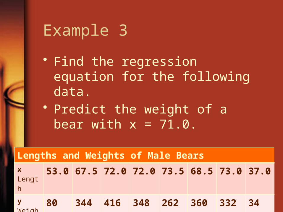
• Find the regression equation for the following data.

• Predict the weight of a bear with x = 71.0.

Lengths and Weights of Male Bearsx Length

53.0 67.5 72.0 72.0 73.5 68.5 73.0 37.0

y Weight

80 344 416 348 262 360 332 34

MATLAB’s “polyfit” (based on minimizing the least-squares of the errors) will serve the purpose.

>> x=[53 67.5 72 72 73.5 68.5 73 37];>> y=[80 344 416 348 262 360 332 34];>> polyfit(x,y,1)ans = 9.6598 -351.6599>>

The equation is y = 9.6598x – 351.6599

MATLAB’s “polyval” can be used to evaluate a value of a polynomial function.

>> x=[53 67.5 72 72 73.5 68.5 73 37];>> y=[80 344 416 348 262 360 332 34];>> polyfit(x,y,1)ans = 9.6598 -351.6599>> polyval(polyfit(x,y,1), 71.0)ans = 334.1849

>>

Multiple regression

• Two or more independent variables.Data from Male Bearsy Weight 80 344 416 348 262 360 332 34x2 Age 19 55 81 115 56 51 68 8x3 Head L 11.0 16.5 15.5 17.0 15.0 13.5 16.0 9.0x4 Head W 5.5 9.0 8.0 10.0 7.5 8.0 9.0 4.5x5 Neck 16.0 28.0 31.0 31.5 26.6 27.0 29.0 13.0x6 Length 53.0 67.5 72.0 72.0 73.5 68.5 73.0 37.0x7 Chest 26 45 54 49 41 49 44 19

y = b1 + b2*x2 + b3*x3 + … + b7*x7

Example 4

• Find b1, b3 and b6.Data from Male Bearsy Weight 80 344 416 348 262 360 332 34x2 Age 19 55 81 115 56 51 68 8x3 Head L 11.0 16.5 15.5 17.0 15.0 13.5 16.0 9.0x4 Head W 5.5 9.0 8.0 10.0 7.5 8.0 9.0 4.5x5 Neck 16.0 28.0 31.0 31.5 26.6 27.0 29.0 13.0x6 Length 53.0 67.5 72.0 72.0 73.5 68.5 73.0 37.0x7 Chest 26 45 54 49 41 49 44 19

y = b1 + b3*x3 + b6*x6

b1 + b3*x3 + b6*x6 = y

b1 + 11.0*b3 + 53.0*b6 = 80b1 + 16.5*b3 + 67.5*b6 = 344b1 + 15.5*b3 + 72.0*b6 = 416b1 + 17.0*b3 + 72.0*b6 = 348b1 + 15.0*b3 + 73.5*b6 = 262b1 + 13.5*b3 + 68.5*b6 = 360b1 + 16.0*b3 + 73.0*b6 = 332b1 + 9.0*b3 + 37.0*b6 = 341 11.0 53.0 801 16.5 67.5 3441 15.5 72.0 b1 4161 17.0 72.0 b3 3481 15.0 73.5 b6 2621 13.5 68.5 3601 16.0 73.0 3321 9.0 37.0 34

=

or AX = y

AX = y[8 by 3][3 by 1] = [8 by 1]

• The problem is – matrix A is not square. We cannot find its inverse and solve the equation as X=A-1y.

X = pinv(A)y[3 by 1] = [3 by 8] [8 by 1]

• I need to have a “3 by 8” matrix which serves like a inverse of A. We call it a pseudo-inverse of matrix A, or pinv(A) = (AtA)-1At .

• See Appendix for the definition of pinv(A)

Pseudo-inverse of matrix A

>> y=[80 344 416 348 262 360 332 34]’;>> x3=[11 16.5 15.5 17 15 13.5 16 9]’;>> x6=[53 67.5 72 72 73.5 68.5 73 37]’;>> A=[ones(size(x3)) x3 x6]

A =

1.0000 11.0000 53.0000 1.0000 16.5000 67.5000 1.0000 15.5000 72.0000 1.0000 17.0000 72.0000 1.0000 15.0000 73.5000 1.0000 13.5000 68.5000 1.0000 16.0000 73.0000 1.0000 9.0000 37.0000

[8 by 3]

Note that y, x3 and x6 must be column vectors.

>> A'*Aans = 1.0e+004 * 0.0008 0.0114 0.0517 0.0114 0.1667 0.7565 0.0517 0.7565 3.4526>> pinvA=inv(ans)*A'

pinvA =0.8763 -0.2719 -0.2571 -0.4628 -0.2293 0.1123 -0.3528 1.5853-0.0983 0.1962 -0.0209 0.1501 -0.1123 -0.1686 0.0132 0.04050.0100 -0.0370 0.0105 -0.0239 0.0302 0.0373 0.0045 -0.0315

>> b=pinvA*yb = -374.3035 18.8204 5.8748>>

[3 by 8] [8 by 3] = [3 by 3]

[3 by 8] = [3 by 3] [3 by 8]

[3 by 1] = [3 by 8] [8 by 1]

y = -374.3035 + 18.8204*x3 + 5.8748*x6

pinv(A) = (AtA)-1At

>> y=[80 344 416 348 262 360 332 34]’;>> x3=[11 16.5 15.5 17 15 13.5 16 9]’;>> x6=[53 67.5 72 72 73.5 68.5 73 37]’;>> A=[ones(size(x3)) x3 x6];>> b=regress(y, A)b = -374.3035 18.8204 5.8748>>

MATLAB’s “regress”

Note that y, x3 and x6 must be column vectors in order to build the 8x3 matrix A.

APPENDIX – LEAST SQUARE METHOD FROM LINEAR ALGEBRA

32

6.4 Least-Squares Curves • We have seen that the system Ax = y of n equations in n

variables, where A is invertible, has the unique solution x = A1y.

• However, if the system has n equations and m variables, with n > m, the system does not, in general, have a solution and it is said to be over-determined.

• A is not a square matrix, thus A1 does not exist.• We will introduce a matrix called the pseudoinverse of A, denoted pinv(A), that leads to a least-squares solution x = pinv(A)y for an over-determined system.

• This is not a true solution, but in some sense the closest we can get in order to have a true solution.

33

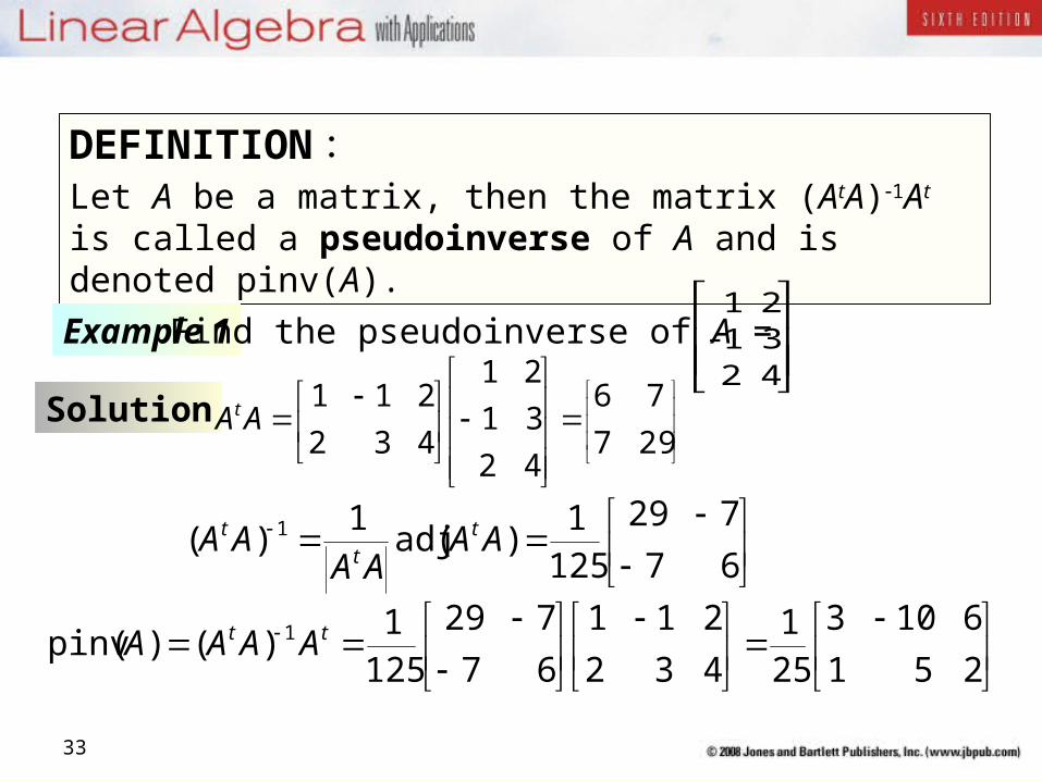
DEFINITION ： Let A be a matrix, then the matrix (AtA)1At is called a pseudoinverse of A and is denoted pinv(A).

Example 1 Find the pseudoinverse of A =

423121

Solution

297

76

42

31

21

432

211AAt

67

729

1251

)(adj1

)( 1 AAAA

AA tt

t

251

6103

251

432

211

67

729

1251

)()(pinv 1 tt AAAA

34

Ax = y x = pinv(A)ysystem least-squares solution

Let Ax = y be a system of n linear equations in m variables with n＞ m, where A is of rank m.

(1) This system has a least-squares solution.

(2) If the system has a unique solution, the least –squares solution is that unique solution.

(3) If the system is over-determined, the least-squares solution is the closest we can get to a true solution.

(4) The system cannot have many solutions.

System of Equations Ax = y

35

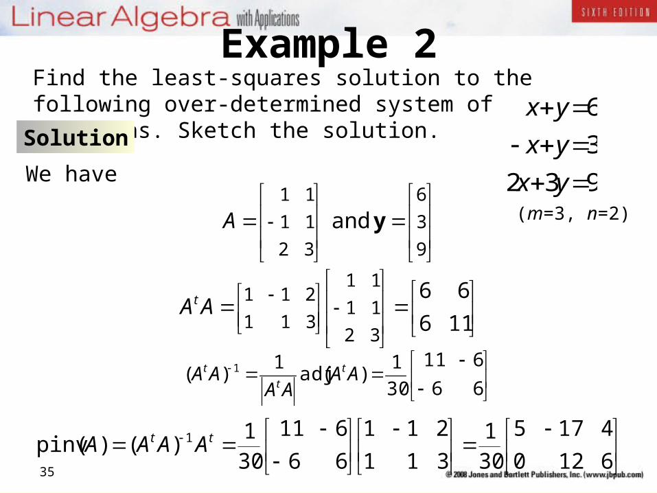
Example 2Find the least-squares solution to the following over-determined system of equations. Sketch the solution.

Solution

932

3

6

yx

yx

yx

We have

9

3

6

32

11

11

and yA

116

66

32

11

11

311

211AAt

66

611

30

1)(adj

1)( 1 AA

AAAA t

t

t

6120

4175

301

311

211

66

611

301

)()(pinv 1 tt AAAA

(m=3, n=2)

36

Then the least-squares solution is

The solution is shown below as point

3

2/1

9

3

6

6120

4175

30

1)(pinv yA

).3 ,(2

1P

37

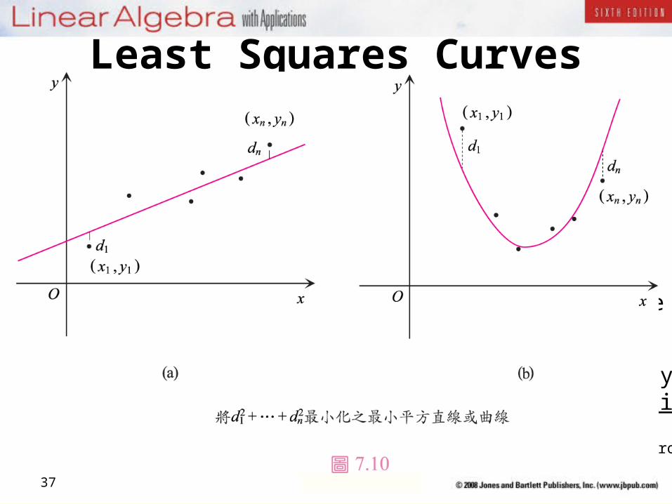
Least Squares Curves

The least squares line or curve can be found by solving a over-determined system. This is found by minimizing the sum ofd1

2 + d22 +…+ dn

2 That’s where we get the name “least squares” from.

Least Squares Line Least Squares Curve

38

Example 3Find the least-squares line for the following data points.

(1, 1), (2, 2.4), (3, 3.6), (4, 4)SolutionLet the equation of the line be y = a + bx. Substituting for these points into the equation, we get an over-determined system:

44633422

1

ba.ba.ba

ba

To solve for the least-squares solution, we have

4

6.3

4.2

1

and

41

31

21

11

yA

Thus

6226

1001020

201

)()(pinv 1 tt AAAA

39

And the least-squares solution is

Thus a = 0.2, b = 1.02.And the equation is

y = 0.2 + 1.02x

02.12.0

62261001020

201

])[(46.34.21

1 ytt AAA

x

y

(1, 1)

(2, 2.4)

(3, 3.6)(4, 4)

40

Example 4Find the least-squares parabola for the following data points.

(1, 7), (2, 2), (3, 1), (4, 3)Solution

Let the parabola be y = a + bx + cx2. Substituting data points:

31641932427

cbacbacbacba

3

1

2

7

and

1641

931

421

111

yA

We have

5555

19272331

152515451

201

)()(pinv tt AAAA

41

Finally we have the solution

Thus a = 15.25, b = 10.05, c = 1.75.

Or

y = 15.25 – 10.05x + 1.75x2

75.1

05.10

25.15

3

1

2

7

5555

19272331

152515451

201

])[( ytt AAA

y = 15.25 – 10.05x + 1.75x2