Singapore Med J 2005; 46(4) : 153

Biostatistics 304.Cluster analysisY H Chan

Faculty of MedicineNational University

of SingaporeBlock MD11Clinical Research

Centre #02-0210 Medical DriveSingapore 117597

Y H Chan, PhDHeadBiostatistics Unit

Correspondence to:Dr Y H ChanTel: (65) 6874 3698Fax: (65) 6778 5743Email: medcyh@nus.edu.sg

CME Article

B a s i c S t a t i s t i c s F o r D o c t o r s

In Cluster analysis, we seek to identify the “natural”structure of groups based on a multivariate profile,if it exists, which both minimises the within-groupvariation and maximises the between-group variation.The objective is to perform data reduction intomanageable bite-sizes which could be used in furtheranalysis or developing hypothesis concerning thenature of the data. It is exploratory, descriptive andnon-inferential.

This technique will always create clusters, be it rightor wrong. The solutions are not unique since theyare dependent on the variables used and how clustermembership is being defined. There are no essentialassumptions required for its use except that there mustbe some regard to theoretical/conceptual rationale uponwhich the variables are selected.

For simplicity, we shall use 10 subjects todemonstrate how cluster analysis works. We areinterested to group these 10 subjects into compliance-on-medication-taking (for example) subgroups basingon four biomarkers, and later to use the clusters todo further analysis – say, to profile compliant vsnon-compliant subjects. The descriptives are givenin Table I, with higher values being indicative ofbetter compliance.

Table I. Descriptive statistics of the biomarkers.

Descriptive statistics

N Minimum Maximum Mean Standarddeviation

x1 10 79.2 87.3 83.870 2.6961

x2 10 73.2 83.3 77.850 3.6567

x3 10 61.8 81.1 72.080 6.4173

x4 10 44.5 51.5 48.950 2.5761

Valid N (listwise)

SPSS offers three separate approaches toCluster analysis, namely: TwoStep, K-Means andHierarchical. We shall discuss the Hierarchicalapproach first. This is chosen when we have little ideaof the data structure. There are two basic hierarchicalclustering procedures – agglomerative or divisive.Agglomerative starts with each object as a clusterand new clusters are combined until eventually allindividuals are grouped into one large cluster. Divisiveproceeds in the opposite direction to agglomerativemethods. For n cases, there will be one-cluster ton-1 cluster solutions.

In SPSS, go to Analyse, Classify, Hierarchical Clusterto get Template I

Template I. Hierarchical cluster analysis.

Put the four biomarkers into the Variable(s) option.If there is a string variable which labels the cases(here “subno’ contains the labels A to J), put “subno”in the Label Cases by option - otherwise, leave it empty.Presently, as we want to cluster the Cases, leave thebullet for Cases checked. Leave the Display for theStatistics and Plots checked. Click on the Statisticsfolder to get Template II.

Singapore Med J 2005; 46(4) : 154

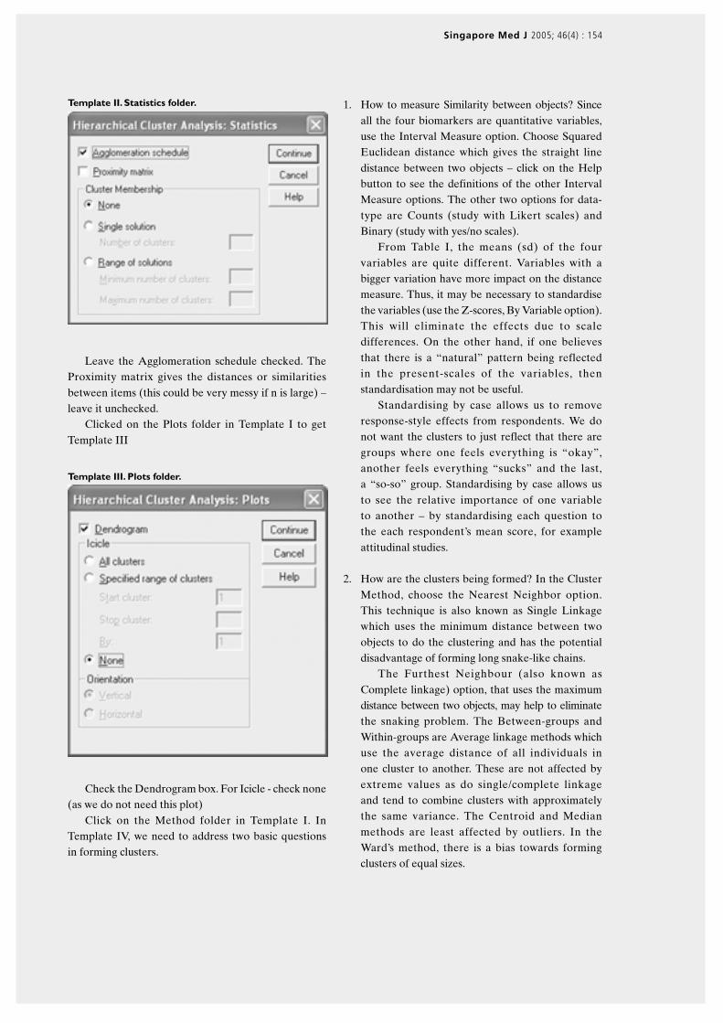
Template II. Statistics folder.

Leave the Agglomeration schedule checked. TheProximity matrix gives the distances or similaritiesbetween items (this could be very messy if n is large) –leave it unchecked.

Clicked on the Plots folder in Template I to getTemplate III

Template III. Plots folder.

Check the Dendrogram box. For Icicle - check none(as we do not need this plot)

Click on the Method folder in Template I. InTemplate IV, we need to address two basic questionsin forming clusters.

1. How to measure Similarity between objects? Sinceall the four biomarkers are quantitative variables,use the Interval Measure option. Choose SquaredEuclidean distance which gives the straight linedistance between two objects – click on the Helpbutton to see the definitions of the other IntervalMeasure options. The other two options for data-type are Counts (study with Likert scales) andBinary (study with yes/no scales).

From Table I, the means (sd) of the fourvariables are quite different. Variables with abigger variation have more impact on the distancemeasure. Thus, it may be necessary to standardisethe variables (use the Z-scores, By Variable option).This will eliminate the effects due to scaledifferences. On the other hand, if one believesthat there is a “natural” pattern being reflectedin the present-scales of the variables, thenstandardisation may not be useful.

Standardising by case allows us to removeresponse-style effects from respondents. We donot want the clusters to just reflect that there aregroups where one feels everything is “okay”,another feels everything “sucks” and the last,a “so-so” group. Standardising by case allows usto see the relative importance of one variableto another – by standardising each question tothe each respondent’s mean score, for exampleattitudinal studies.

2. How are the clusters being formed? In the ClusterMethod, choose the Nearest Neighbor option.This technique is also known as Single Linkagewhich uses the minimum distance between twoobjects to do the clustering and has the potentialdisadvantage of forming long snake-like chains.

The Furthest Neighbour (also known asComplete linkage) option, that uses the maximumdistance between two objects, may help to eliminatethe snaking problem. The Between-groups andWithin-groups are Average linkage methods whichuse the average distance of all individuals inone cluster to another. These are not affected byextreme values as do single/complete linkageand tend to combine clusters with approximatelythe same variance. The Centroid and Medianmethods are least affected by outliers. In theWard’s method, there is a bias towards formingclusters of equal sizes.

Singapore Med J 2005; 46(4) : 155

Template IV. Method folder.

The output of the above analysis will only haveone table (Table II) and one figure (Fig. 1)

Table II shows the Agglomeration schedule,using Squared Euclidean distance (standardised)measure and Nearest-Neighbor (Single linkage)cluster. This displays the cases or clusters combinedat each stage, the distances between the cases orclusters being combined, and the last cluster levelat which a case joined the cluster.

Under the Cluster Combined columns, the firsttwo subjects to be clustered are 5 & 10, then 3 & 6,then 1 & 7, then (3 & 6) with subject 2, etc. TheCoefficients column shows the distance where theclusters were being formed. The information givenin the Stage Clusters First Appears columns justindicates when an object is joining an existingcluster or when two existing clusters are beingcombined. This table shows the numerical illustrationof the clustering.

The dendrogram (Fig. 1) is the graphical equivalentof the Agglomeration schedule.

Table II. Agglomeration schedule, nearest neighbor (single linkage) and squared euclidean distance (standardised).

Agglomeration schedule

Cluster combined Stage cluster first appears

Stage Cluster 1 Cluster 2 Coefficients Cluster 1 Cluster 2 Next stage

1 5 10 .689 0 0 8

2 3 6 1.046 0 0 4

3 1 7 1.724 0 0 7

4 2 3 1.920 0 2 5

5 2 4 2.150 4 0 6

6 2 8 3.338 5 0 7

7 1 2 3.376 3 6 8

8 1 5 4.818 7 1 9

9 1 9 7.451 8 0 0

Fig. 1 Dendrogram using single linkage.

Rescaled distance cluster combine

Singapore Med J 2005; 46(4) : 156

A picture tells a thousand words! The dendrogramshows that we have an outlier (subject 9, label I) – known asa Runt or Entropy group, which is completely on its own.

The third and final question in Cluster Analysis is:how many clusters are to be formed?

A possible three cluster solution is subject 9(label I) with two clusters, [B,C,F,D,A,G,H] and [E,J].Another possibility is four clusters with [I], [A,G] , [E,J]and [B,C,F,D,H]. We can save the cluster membershipby clicking on the Save folder in Template I – seeTemplate V. If we decide to have four clusters afterstudying the dendrogram, choose the Single solutionand Number of clusters = 4. SPSS will create a newvariable CLU4_1 in the dataset. Perhaps, we want todo further exploration with different cluster solutions;we could use the Range of solutions option: Minimum= 2 and Maximum = 4, for example. SPSS will createthree new variables CLU4_1, CLU3_1 and CLU2_1for the 4, 3 & 2 cluster memberships, respectively.

Are we done? Things are not that simple (that’slife!) What happens if we decide to use anotherprocedure to form the clusters, say, Furthest Neighbour(also known as Complete Linkage) and stick to theSquared Euclidean distance measure? We will onlyshow the dendrogram solution (Fig. 2)

A completely different set of solutions!It is probably clear by now that the selection of the

final cluster solution is dependent on the researcher’sjudgment, given that the relevant variables havebeen used! One could try the other possibilities ofsimilarity measures and cluster-linkage options toexplore the data.

Cluster analysis could also be performed on thevariables instead of objects. In Template I, choose theCluster Variables option. Fig. 3 shows the dendrogramwith Standardised Eluclidean distance and NearestNeighbour for the clustering of the variables.

Fig. 2 Dendrogram using complete linkage.

Rescaled distance cluster combine

Template V. Saving the cluster membership.

Singapore Med J 2005; 46(4) : 157

The K-Means (also known as Quick Cluster) analysiscould be used if we know the number of clusters to beobtained. This technique is non-hierarchical whichdoes not involve the dendrogram-type of construction.Each cluster has an initial centre and objects withina pre-specified distance are included in the resultingcluster. Clusters’ centres are updated, objects may bereassigned, and the process continues until all objectsare duly classified to a cluster.

Template VI shows the options for a K-Meansclustering. Number of clusters = 4 (say), choose Iterateand classify Method to allow for the objects to be“reclassified” during the clustering process. Leave the“Cluster Centres: Read initial from” unchecked – thiswill let the program to choose its own random clusterinitial centre. Different results could be obtained whendifferent cluster initial centres are being used! Note thatK-Means do not standardise the variables for us. Wewill have to do it on our own using Analyze, DescriptiveStatistics, Descriptive – save standardised values asvariables option.

Template VI. K-Means cluster analysis.

Click on Iterate folder to specify the number ofiterations required (Template VII).

Template VII. Maximum number of iterations declared.

Click on the Save folder for Cluster membership(Template VIII).

Template VIII. K-Means: saving cluster membership.

Click on the Option folder in Template VI. Checkall the boxes for Statistics, and Exclude cases pairwisefor Missing Values (this will make use of all availablenon-missing data), see Template IX.

Fig. 3 Dendrogram for cluster of variables – single linkage, standardised squared euclidean distance.

Rescaled distance cluster combine

Singapore Med J 2005; 46(4) : 158

Template IX. K-Means options.

Tables IIIa-g show the outputs in a K-Meansanalysis. Table IIIa shows the starting cluster initialcentres with Table IIIb showing that the iterationcompleted at the second run (where all the numbersare small). When we have more cases to be clustered,the iteration process may take longer and we have tochange the maximum of number of iterations inTemplate VII to a higher number. We could also savethe last unconverged cluster centres in a file to beserved as the initial cluster centres for the next run ofthe process - this is done by checking the “Clustercentres: Write final as” button in Template VI.

The following results (Tables IIIc-g) could only beused when the iteration process converges. TableIIIc shows the cluster membership with Table IIIdspecifying the final cluster centres. Table IIIe showsthe Squared Euclidean distances (the only optionavailable in K-Means) between the clusters. TableIIIf shows which variables are significantly differentamongst the clusters and Table IIIg gives the numberof objects in each cluster.

Table IIIa. Initial cluster centres.

Initial cluster centres

Cluster

1 2 3 4

x1 82.5 79.2 86.9 86.1

x2 76.1 73.2 80.3 83.3

x3 61.8 72.3 71.5 81.1

x4 51.0 44.5 49.0 51.0

Table IIIb. Iteration history.

Iteration history

Change in cluster centres

Iteration 1 2 3 4

1 3.294 3.903 2.032 4.055

2 .000 .000 .000 .000

Table IIIc. K-Means: cluster membership.

Cluster membership

Case number Subno Cluster Distance

1 A 1 3.323

2 B 3 2.032

3 C 3 2.032

4 D 4 4.055

5 E 4 6.005

6 F 4 4.127

7 G 1 3.294

8 H 1 3.976

9 I 2 3.903

10 J 2 3.903

Table IIId. Final cluster centres.

Final cluster centres

Cluster

1 2 3 4

x1 84.2 80.2 85.5 85.0

x2 76.5 73.4 80.9 80.2

x3 63.9 73.7 72.4 79.0

x4 49.2 48.0 48.0 50.0

Table IIIe. Distances between final cluster centres.

Distances between final cluster centres

Cluster

Cluster 1 2 3 4

x1 11.064 9.632 15.525

x2 11.064 9.254 10.069

x3 9.632 9.254 6.960

x4 15.525 10.069 6.960

Table IIIf. ANOVA table for each variable by clusters.

ANOVA

Cluster Error

Mean df Mean df F Sig.square square

x1 11.934 3 4.936 6 2.418 .165

x2 26.845 3 6.635 6 4.046 .069

x3 115.593 3 3.976 6 29.070 .001

x4 2.353 3 8.778 6 .268 .846

Singapore Med J 2005; 46(4) : 159

Table IIIg. Number of cases in each cluster.

Number of cases in each cluster

Cluster 1 3.000

2 2.000

3 2.000

4 3.000

Valid 10.000

Missing .000

The Two-Step Cluster (see Template X) analysisallows us to have a combination of continuous andcategorical variables which both hierarchical andK-means procedures do not cater for. It also allowsus to specify the number of clusters required or tolet the program to decide the optimal numberof clusters.

When all the variables are continuous, theEuclidean Distance Measure is used. These variableswill be standardised during the analysis. When acombination of continuous and categorical variablesare used, the Log-likelihood distance measure haveto be used. This likelihood distance measure assumesthat variables in the cluster model are independentwith all continuous variables assumed to have anormal distribution and all categorical variables tohave a multinomial distribution. Fortunately theTwo-Step procedure is fairly robust to violations ofboth the assumption of independence and thedistributional assumptions.

We will not generate any output results for thisprocedure. Those who are interested could click on

the Help button in Template X to see a completeillustration of cluster analysis using the Two-Stepprocedure.

Template X. Two-step cluster analysis.

In conclusion, we have to bear in mind that Clusteranalysis is an exploratory technique where we hopeto find distinct groups based on a multivariate profile.It is an art rather than a science. However, it can bean invaluable tool to identify latent patterns in a hugedataset that could not be discerned by any othermultivariate statistical method.

SINGAPORE MEDICAL COUNCIL CATEGORY 3B CME PROGRAMMEMultiple Choice Questions (Code SMJ 200504A)

True False

Question 1. Which cluster-linkage method in the hierarchical technique has a potential to produce snakelike clusters?(a) The Single linkage. � �(b) The Complete linkage. � �(c) The Ward’s linkage. � �(d) The Centroid linkage. � �

Question 2. Which cluster-linkage method in the hierarchical technique is not affected by outliers?(a) The Single linkage. � �(b) The Complete linkage. � �(c) The Average linkage. � �(d) The Centroid linkage. � �

Question 3. Which technique provides a dendrogram?(a) The Hierarchical technique. � �(b) The K-means technique. � �(c) The Two-Step technique. � �(d) All of the above. � �

Question 4. Which technique could determine the optimal number of clusters for us automatically?(a) The Hierarchical technique. � �(b) The K-means technique. � �(c) The Two-Step technique. � �(d) All of the above. � �

Question 5. Which of the following statements are true?(a) K-Means is a non-hierarchical technique. � �(b) Results from Cluster analysis are unique. � �(c) Continuous variables must be standardised before clustering. � �(d) Clusters will always be created. � �

Doctor’s particulars:

Name in full: _______________________________________________________________________________________

MCR number: ______________________________________ Specialty: ______________________________________

Email address: ______________________________________________________________________________________

Submission instructions:A. Using this answer form1. Photocopy this answer form.2. Indicate your responses by marking the “True” or “False” box �3. Fill in your professional particulars.4. Either post the answer form to the SMJ at 2 College Road, Singapore 169850 OR fax to SMJ at (65) 6224 7827.

B. Electronic submission1. Log on at the SMJ website: URL http://www.sma.org.sg/cme/smj2. Either download the answer form and submit to smj.cme@sma.org.sg OR download and print out the answer form for this

article and follow steps A. 2-4 (above) OR complete and submit the answer form online.

Deadline for submission: (April 2005 SMJ 3B CME programme): 12 noon, 25 May 2005Results:1. Answers will be published in the SMJ June 2005 issue.2. The MCR numbers of successful candidates will be posted online at http://www.sma.org.sg/cme/smj by 20 June 2005.3. Passing mark is 60%. No mark will be deducted for incorrect answers.4. The SMJ editorial office will submit the list of successful candidates to the Singapore Medical Council.

✓

Singapore Med J 2005; 46(4) : 160