biogenic volatile organic compoud emissions in some...
TRANSCRIPT

Biogenic volatile organic compound emissions in grassland and forests in China
(I) and Variations of trace gases and particulate matter at Xinglong station (II)
Bai Jianhui1, Guenther Alex2,3, Turnipseed Andrew2
, Duhl Tiffany2, Greenberg James2, Wan Xiaowei1, van der A Ronald4, Yu Shuquan5
, Wang Bin5, Hao Nan6, Wang PuCai1 1. LAGEO, Institute of Atmospheric Physics, Chinese Academy of Sciences, Beijing 100029 2. National Center for Atmospheric Research, Boulder, CO 80307, USA 3. Now at Pacific Northwest National Laboratory, Richland WA 99352, USA and Washington State University, Pullman WA
99164, USA 4. KNMI, Utrechtseweg 297, 3731GA De Bilt, The Netherlands. 5.School of Forestry & Bio-technology Zhejiang Agriculture and Forestry University,Hangzhou 311300. 6. German Aerospace Center (DLR), 82234, Wessling, Germany.

1. Introduction BVOC emissions (I)
BVOCs play important roles in: O3 photochemistry the formation of secondary organic aerosols (SOA,PM2.5) the Carbon budget BVOCs’ oxidation influences OH radicals and O3 BVOCs take part in chemical and photochemical reactions in the atmosphere, consume solar UV and visible radiation directly and/or indirectly
BVOC emission studies in some ecosystems in China are summarized, so as to understand their emission characteristics. More studies are needed in the future.

1) Changbai Mountain temperate forest (42o24’N,128o6’E, 738m
asl), jilin province, in 2010 and 2011 growing seasons REA (Relaxed Eddy Accumulation) technique Dominant trees:
Pinus koraiensis, Tilia amurensis, Quercus mongolica, Fraxinus mandshurica, Acer mono. Dominant Shrubs:
Deutzia amurensis, Acer pseudosieboldiarum, A. Tegmentosum, Corylus mandshurica.
2) Subtropical bamboo forest at Taihuyuan (30o18’N, 119o34’E) in
Linan city, Zhejing province, from July 2012 to January 2013. REA technique Dominant species: Phyllostachysviolascens or Lei bamboo
2. BVOC flux measurements in some ecosystems in China 2.1 Site description

3) Inner Mongolia grassland (43o26’- 44o08’N,116o04’ - 117o05’E) Ecosystem Research Station, CAS, in 2002 and 2003 growing seasons. Chamber method: 90cm×90cm×35cm Dominant species: A. chinense, Achnatherum sibiricum, S. grandis, Carex appendiculata, K. cristata, C. squarrosa, A. senescens, and A. tenuissimum.
4) Qianyanzhou subtropical forest (26o44’N, 115o03’E) in Taihe county, Jiangxi province from Jan., 2013 to Dec., 2015.
REA technique
Dominant species :
Pinus elliottii, Pinus massoniana · ·
· ·

Changbai Mountain temperate forest Qianyanzhou subtropical forest
LinAn subtropical bamboo forest
O3 analyzer
Solar radiation system

• Measuring time period: Growing seasons (e.g., 28 June to 25 August, 2010 in Changbai
temperate forest). • Air sample collections: 1) diurnal variation:6,9,12,15,18; 2) day-day variation: around noon • Sample analysis: The sampled cartridges were analyzed by GC-FID and GC-MS. Flux calculation: F = bσw(Cup-Cdown) (1) b: a proportionality factor; σw: standard deviation of the vertical
wind speed; Cup-Cdown : concentration difference between the updraft and downdraft cartridges over a period of 30 min.
2.3 Measurement of Solar radiation
2.2 Observation and analysis of BVOCs
Global solar radiation (Q): 270-3200 nm Direct radiation (D): 270-3200 nm Scattered radiation (S): Q - D PAR (photosynthetically active radiation): 400-700 nm (Licor)

1) Main VOC species in Changbai temperate forest: isoprene, αpinene,βpinene, camphene, sabinene, myrcene, carene, limonene, ocimene, terpinene, cymene, terpinolene, tricyclene.
The mean isoprene emission flux (mgm-2h-1) was 0.889, mean total monoterpene emission flux was 0.143 in 2011 summer.
2.4 Measuring results
-1
0
1
2
3
4
5
6
2011-06-1913:00
2011-06-2014:00
2011-06-2106:00
2011-06-2112:00
2011-06-2118:00
2011-06-2413:30
2011-06-2611:30
2011-06-2613:30
2011-06-2814:30
2011-06-3009:00
2011-06-3015:30
2011-07-1014:30
2011-07-1109:00
2011-07-1115:00
2011-07-1212:00
2011-07-1313:00
2011-07-1411:00
2011-07-1413:00
2011-07-1514:00
2011-07-1516:00
2011-07-1609:00
2011-07-1615:00
2011-07-2213:00
2011-07-2314:00
2011-07-2406:00
2011-07-2412:00
2011-07-2418:00
2011-07-2509:00
2011-07-2511:00
2011-07-2614:30
2011-07-2815:00
2011-07-2909:00
2011-07-2915:00
2011-09-0506:00
2011-09-0509:00
2011-09-0512:00
2011-09-0515:00
2011-09-0517:30
2011-09-0610:00
2011-09-0614:00
2011-09-0709:00
2011-09-0715:00
2011-09-0811:00
2011-09-0814:00
Date Time
Isop
rene
em
issi
on f
lux
(mgm-2
h-1),
PA
R (
mol
m-2)
0
5
10
15
20
25
30
35
T (℃
)
isoprene PAR T
Fig.1 Isoprene emission flux, PAR,T in 2011 summer at a temperate forest in China

2) Main VOC species in a subtropical Lei bamboo forest The mean isoprene emission flux was 0.95 mgm-2h-1(maximum-10.32), the total monoterpene emission flux was 0.012 mgm-2h-1 from 7 July, 2012 to 19 Jan., 2013. α-pinene (-0.34 - 0.12), longifolene (-0.01-0.03), α-cadrene (-0.004 - 0.001) mgm-2h-1
-2
0
2
4
6
8
10
12
2012
-07-
0714
:00
2012
-07-
0809
:00
2012
-07-
0814
:00
2012
-07-
0911
:00
2012
-07-
0913
:00
2012
-07-
1006
:00
2012
-07-
1012
:00
2012
-07-
1018
:00
2012
-07-
1112
:30
2012
-07-
1213
:30
2012
-07-
1215
:30
2012
-07-
1309
:00
2012
-07-
1315
:00
2012
-08-
2009
:00
2012
-08-
2011
:00
2012
-08-
2013
:00
2012
-08-
2015
:00
2012
-08-
2211
:00
2012
-08-
2213
:00
2012
-08-
2311
:00
2012
-08-
2313
:00
2012
-08-
2411
:00
2012
-08-
2506
:00
2012
-08-
2512
:00
2012
-08-
2518
:00
2012
-08-
2609
:00
2012
-08-
2615
:00
2012
-09-
2516
:00
2012
-09-
2608
:00
2012
-09-
2610
:00
2012
-09-
2612
:00
2012
-09-
2614
:00
2012
-09-
2616
:00
2012
-09-
2706
:00
2012
-09-
2712
:00
2012
-09-
2718
:00
2012
-09-
2812
:30
2012
-09-
2910
:30
2012
-09-
3009
:00
2012
-09-
3015
:00
2012
-10-
0114
:00
2012
-10-
2812
:00
2012
-10-
2814
:00
2012
-10-
3114
:00
2012
-11-
0112
:00
2012
-11-
0114
:00
2012
-11-
0116
:00
2012
-11-
0210
:00
2012
-11-
0212
:00
2012
-11-
0214
:00
2012
-11-
0312
:00
2012
-11-
0512
:30
2012
-11-
0514
:00
2013
-01-
1809
:00
2013
-01-
1812
:30
2013
-01-
1814
:30
2013
-01-
1912
:00
2013
-01-
1914
:00
Date and Time
Emiss
ion
flux
(mgm-2
h-1) ISOmea
Fig. 2 The measured emission fluxes of isoprene at a subtropical Lei bamboo forest in China

3. Empirical models and their simulations 3.1 Empirical models of isoprene and monoterpene emissions PAR/cosZ = A1’e-k1Etm + A2’e-kwm + A3’e-S/Q + A0’ (2) (1) e-k1Etm: PAR attenuation by isoprene/monoterpene through OH radical during the photochemical reactions. (2) e-K2Wm: PAR absorption and/or utilization by gases, liquids, particles (GLPs) trough OH radicals. (3) e-S/D: Total scattering effects by GLPs in the atmosphere. Ai’ are empirical coefficients (i=1,2,3,0). Isoprene and monoterpene emission flux can be calculated by: e-k1Etm = A1PAR/cosZ + A2e-kwm + A3e-S/Q + A0 (3)

Fig. 3 Observed and calculated (‘obs’and ‘cal’, respectively) isoprene emission fluxes in Changbai temperate forest
Fig. 4 Observed and calculated mean "diurnal variation" of isoprene for 2010 and 2011 growing seasons in Changbai temperate forest
0
0.5
1
1.5
2
2.5
3
2010-0
7-0
9 1
2:3
0
2010-0
7-2
4 1
2:0
0
2010-0
7-2
9 1
2:3
0
2010-0
7-3
0 0
9:3
0
2010-0
8-1
2 0
9:3
0
2010-0
8-1
7 1
4:0
0
2010-0
8-2
5 1
3:0
0
2011-0
6-2
0 1
4:3
0
2011-0
6-2
1 1
2:3
0
2011-0
6-2
4 1
4:0
0
2011-0
7-1
0 1
4:3
0
2011-0
7-1
2 1
2:3
0
2011-0
7-1
4 1
2:0
0
2011-0
7-1
4 1
4:0
0
2011-0
7-2
4 1
5:3
0
2011-0
7-2
8 1
5:3
0
2011-0
9-0
6 1
2:3
0Date Time
Em
issi
on f
lux (
mgm-2
h-1
)
Isoprene calIsoprene obs
00.5
11.5
22.5
3
6:3
0
9:3
0
11
:30
12
:00
12
:30
13
:00
13
:30
14
:00
14
:30
15
:00
15
:30
Time
Em
issi
on
flu
x (
mg
m-2h
-1)
Isoprene calIsopreno obs
3.2 Simulation results
• Isoprene model can capture most diurnal variation patterns of isoprene

-1
0
1
2
3
4
5
06-
19 0
6:00
06-
20 0
6:00
06-
21 0
6:00
06-
22 0
6:00
06-
23 0
6:00
06-
24 0
6:00
06-
25 0
6:00
06-
26 0
6:00
06-
27 0
6:00
06-
28 0
6:00
06-
29 0
6:00
06-
30 0
6:00
07-
01 0
6:00
07-
02 0
6:00
07-
03 0
6:00
07-
04 0
6:00
07-
05 0
6:00
07-
06 0
6:00
07-
07 0
6:00
07-
08 0
6:00
07-
09 0
6:00
07-
10 0
6:00
07-
11 0
6:00
07-
12 0
6:00
07-
13 0
6:00
07-
14 0
6:00
07-
15 0
6:00
07-
16 0
6:00
07-
17 0
6:00
07-
18 0
6:00
07-
19 0
6:00
07-
20 0
6:00
07-
21 0
6:00
07-
22 0
6:00
07-
23 0
6:00
07-
24 0
6:00
07-
25 0
6:00
07-
26 0
6:00
07-
27 0
6:00
07-
28 0
6:00
07-
29 0
6:00
07-
30 0
6:00
07-
31 0
6:00
08-
01 0
6:00
08-
02 0
6:00
08-
03 0
6:00
08-
04 0
6:00
08-
05 0
6:00
08-
06 0
6:00
08-
07 0
6:00
08-
08 0
6:00
08-
09 0
6:00
08-
10 0
6:00
08-
11 0
6:00
08-
12 0
6:00
08-
13 0
6:00
08-
14 0
6:00
08-
15 0
6:00
08-
16 0
6:00
08-
17 0
6:00
08-
18 0
6:00
08-
19 0
6:00
08-
20 0
6:00
08-
21 0
6:00
08-
22 0
6:00
08-
23 0
6:00
08-
24 0
6:00
08-
25 0
6:00
08-
26 0
6:00
08-
27 0
6:00
08-
28 0
6:00
08-
29 0
6:00
08-
30 0
6:00
08-
31 0
6:00
09-
01 0
6:00
09-
02 0
6:00
09-
03 0
6:00
09-
04 0
6:00
09-
05 0
6:00
09-
06 0
6:00
09-
07 0
6:00
09-
08 0
6:00
Date Time
Emis
sion
(mgm
-2)
Iso 3F Iso 2F Iso obs Iso M
Fig. 5 Isoprene simulations by using empirical models (3-Factor, 2-Factor ), MEGAN model (Iso 3F, Iso 2F, Iso M) and measured emissions (Iso obs) in 2011 growing season in Changbai temperate forest. • Mean hourly emissions in 2010 and 2011 growing seasons: 1.71 and 1.55 mgm-2h-1 for isoprene, 0.48 and 0.47 mgm-2h-1 for monoterpenes.
3.2 Simulation results:hourly emission

-0.4
-0.2
0
0.2
0.4
0.6
0.8
1
1.2
1.4
1.6
2011-0
6 01:0
0
2011-0
6 05:0
0201
1-06 0
9:00
2011-0
6 13:0
0201
1-06 1
7:00
2011-0
6 21:0
0201
1-07 0
1:00
2011-0
7 05:0
0201
1-07 0
9:00
2011-0
7 13:0
0
2011-0
7 17:0
0201
1-07 2
1:00
2011-0
8 01:0
0201
1-08 0
5:00
2011-0
8 09:0
0201
1-08 1
3:00
2011-0
8 17:0
0201
1-08 2
1:00
2011-0
9 01:0
0201
1-09 0
5:00
2011-0
9 09:0
0
2011-0
9 13:0
0201
1-09 1
7:00
2011-0
9 21:0
0
Date Time
Isopre
ne em
ission
(mgm
-2 )
Iso 2FIso 3FIso M
Fig. 6 Monthly mean diurnal variations of isoprene emission in 2011 growing season in Changbai Mountain temperate forest
3.2 Simulation results: monthly mean diurnal variation
• Total emission in growing season:
isoprene=1239.1, MT=340.4 (2011); isoprene=1283.5, MT=349.7 mgm-2 (2010)
The emission decreases of isoprene and monoterpenes (MT) from 2010 to 2011 associated with the temperature decreasing by -6.6% and water vapor decreasing by -7.6%, PAR increasing by 8.5% and S/Q increasing by 3.8%.
• Similar simulations of isoprene and monoterpene emissions were obtained in subtropical bamboo forest as Changbai Mountain temperate forest.

3.4 Isoprene emission model in the Inner Mongolia grassland
e-k1Et/m = -0.12 PAR +0.07 e-k2wm -0.003e-S/D +0.96 (4)
-500
0
500
1000
1500
2000
2002
-06-26
09:00
2002
-06-26
11:00
2002
-06-26
13:00
2002
-06-26
15:00
2002
-06-27
08:00
2002
-06-27
10:00
2002
-06-27
12:00
2002
-06-27
14:00
2002
-06-28
08:00
2002
-06-28
10:00
2002
-06-28
12:00
2002
-06-28
14:00
2002
-08-13
08:40
2002
-08-13
11:00
2002
-08-13
13:00
2002
-08-15
08:50
2002
-08-15
11:00
2002
-08-15
13:00
2002
-08-15
15:00
2002
-08-16
08:30
2002
-08-16
11:00
2002
-08-16
13:00
2002
-08-16
15:00
2002
-08-31
08:40
2002
-08-31
11:00
2002
-08-31
13:00
2002
-08-31
15:00
2002
-09-02
08:50
2002
-09-02
11:00
2002
-09-02
13:00
2002
-09-03
08:30
2002
-09-03
11:00
2002
-09-03
13:00
2003
-09-02
11:00
2003
-09-02
12:38
2003
-09-02
14:20
2003
-09-02
16:09
2003
-09-03
11:10
2003
-09-03
13:10
2003
-09-03
15:10
Date-time
Emiss
ion flu
x (μg
C m-2
h-1) calculated
measured
Fig. 7 The calculated and measured emission fluxes of isoprene in 2002 and 2003 in the Inner Mongolia grassland
• Simulation result: the relative biases of 65% estimated emissions were within 50% of measured fluxes.
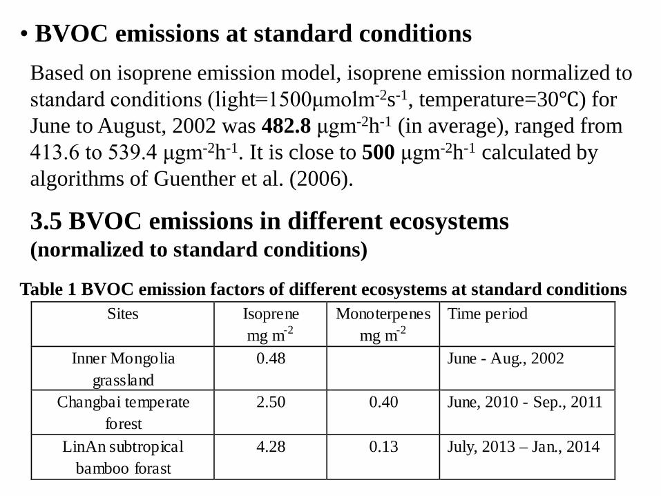
• BVOC emissions at standard conditions
Sites Isoprene mg m-2
Monoterpenes mg m-2
Time period
Inner Mongolia grassland
0.48
June - Aug., 2002
Changbai temperate forest
2.50 0.40 June, 2010 - Sep., 2011
LinAn subtropical bamboo forast
4.28 0.13 July, 2013 – Jan., 2014
3.5 BVOC emissions in different ecosystems (normalized to standard conditions)
Based on isoprene emission model, isoprene emission normalized to standard conditions (light=1500μmolm-2s-1, temperature=30℃) for June to August, 2002 was 482.8 μgm-2h-1 (in average), ranged from 413.6 to 539.4 μgm-2h-1. It is close to 500 μgm-2h-1 calculated by algorithms of Guenther et al. (2006).
Table 1 BVOC emission factors of different ecosystems at standard conditions

4. GC-FID system/technique for BVOC analysis (collaborated with James Greenberg, NCAR, USA)

y = 23.717xR2 = 0.9829
0
100000
200000
300000
400000
500000
0 5000 10000 15000 20000
Area
Con
cent
ratio
n*V
olum
e
Fig. 8 Concentration*Volume vs area using heptane as a standard gas, Response factor=23.717
4.1 Response factor was determined by analyzing heptane and diluting it from 10.4 ppm to different concentrations

4.2 Good reproducibility was obtained by analyzing isoprene and monoterpene mixtures
Run 1
Run 2
Isoprene α- pinene
β-pinene
camphene
limonene
Fig. 9 Gas chromatogram of BVOCs

Species Retention Time
Peak Area Run 1
Peak Area Run 2
Ratio of peak area Run2/Run1
Isoprene 5.557 66792 66222 0.991 α-pinene 14.143 51676.1 51395.7 0.995 camphene 14.574 60780 60633.1 0.998 β-pinene 15.115 62743.7 62623.8 0.998 limonene 15.955 118999 120311 1.011
• Reproducibility of identified BVOCs by using GC-FID
• BVOC emissions emitted form Qianyanzhou subtropical plantations limonene
Isoprene
• Higher limonene emission than isoprene.
• Dominant trees: pinus elliottii, Pinus massoniana.
Table 2. Retention time, peak areas of BVOCs and their ratios for 2 runs
Fig. 10 Gas chromatogram of BVOCs in Qianyanzhou forest

5. Routine observations of trace gases, solar radiation, meteorological parameters, particles, AOD
1) Trace gases – (O3, NO, NO2, SO2), solar radiation (including solar global radiation, solar direct and scattered radiation, UV, PAR, etc.), meteorological parameters, particles (PM2.5), AOD were carried out at some sites in China.
These sites include Xinglong station and Xianghe station in Hebei province. Changbai Mountaians forest in Jilin province, Linan bamboon forest in Zhejiang province, Qianyanzhou forest in Jiangxi province. 2) Some surface measurements of trace gases and particles were provided for the validation
of models. Good results were achieved.
Qianyanzhou station Qianyanzhou station Xinglong station
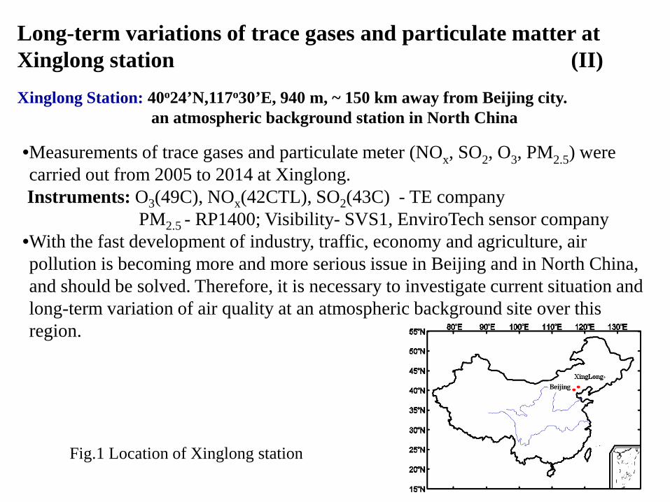
•Measurements of trace gases and particulate meter (NOx, SO2, O3, PM2.5) were carried out from 2005 to 2014 at Xinglong.
Instruments: O3(49C), NOx(42CTL), SO2(43C) - TE company PM2.5 - RP1400; Visibility- SVS1, EnviroTech sensor company •With the fast development of industry, traffic, economy and agriculture, air pollution is becoming more and more serious issue in Beijing and in North China, and should be solved. Therefore, it is necessary to investigate current situation and long-term variation of air quality at an atmospheric background site over this region.
Long-term variations of trace gases and particulate matter at Xinglong station (II) Xinglong Station: 40o24’N,117o30’E, 940 m, ~ 150 km away from Beijing city. an atmospheric background station in North China
Fig.1 Location of Xinglong station
0
10
20
30
40
50
60
70
80
90
100
0
5
10
15
20
25
200505
200509
200601
200605
200609
200701
200705
200709
200801
200805
200809
200901
200905
200909
201001
201005
201009
201101
201105
201109
201201
201205
201209
201301
201305
201309
201401
201405
201409
201501
O3 (ppb)
NO,NO2,SO2 (ppb)
Year month
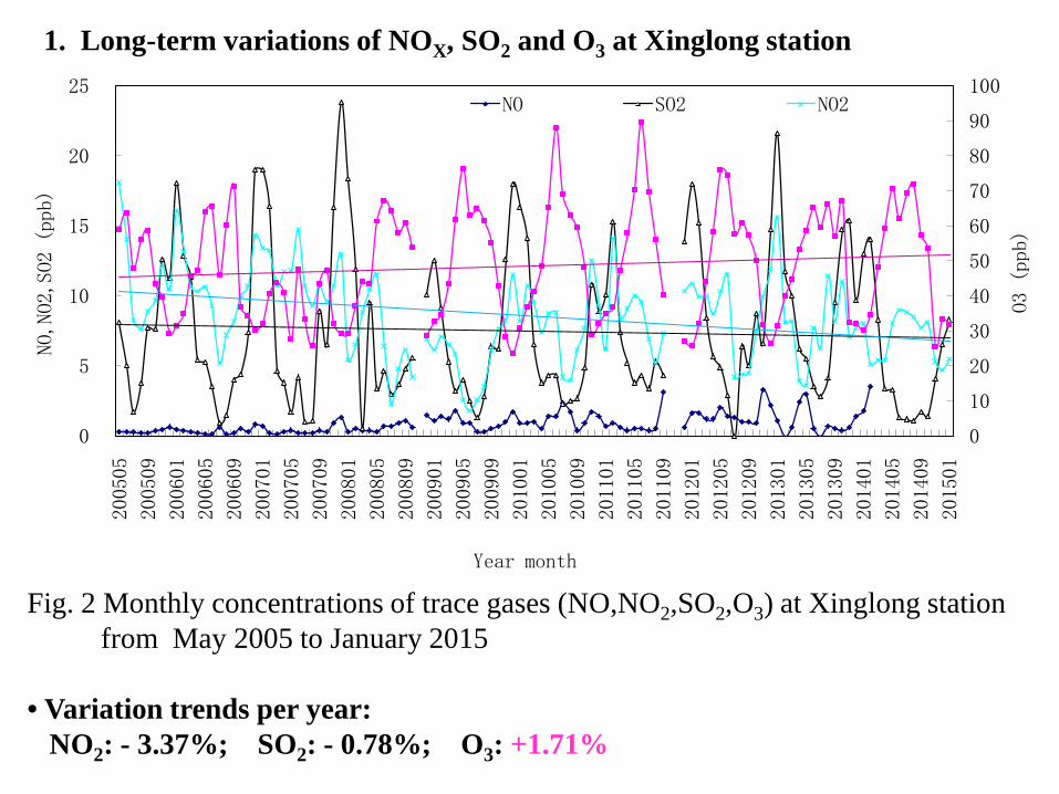
NO SO2 NO2
Fig. 2 Monthly concentrations of trace gases (NO,NO2,SO2,O3) at Xinglong station from May 2005 to January 2015 • Variation trends per year: NO2: - 3.37%; SO2: - 0.78%; O3: +1.71%
1. Long-term variations of NOX, SO2 and O3 at Xinglong station

Fig. 3 Annual mean concentrations of particulate mater(PM2.5)at Xinglong station from 2009 to 2015 • PM2.5 indicated an increase trend at the rate of 0.91% per year.
y = 0.3562x + 39.21
R² = 0.0247
25
30
35
40
45
50
200
9
201
0
201
1
201
2
201
3
201
4
PM (μ
g·m
-3)
Year
2. Long-term variations of particulate mater(PM2.5)at Xinglong station

3. Mechanism analysis: why NO2 and SO2 decrease, PM2.5 increase? AVOCs+BVOCs + OH + other GLPs (NO2,SO2…) → New GLPs(O3, PAN, PM2.5…) • To control air pollution in Beijing and North China, we should 1) control all source emissions of anthropogenic volatile organic
compounds (AVOCs) primarily 2) control all source emissions of NOx and SO2, so as to decrease
the reactants taking part in the chemical and photochemical reactions in the atmosphere and the formation of secondary pollutants, e.g., O3 and PM2.5.
Fig. 4 The car number and planting area in Beijing region from 1978 to 2014 0.0E+00
2.0E+09
4.0E+09
6.0E+09
8.0E+09
1.0E+10
1.2E+10
0.0E+00
1.0E+06
2.0E+06
3.0E+06
4.0E+06
5.0E+06
6.0E+06
1978
1981
1984
1987
1990
1993
1996
1999
2002
2005
2008
2011
2014
Planting area (m2 )
Car number
Year
Car number
Planting Area

-2000
0
2000
4000
6000
8000
10000
12000
0
20
40
60
80
100
120
2005
05
2005
09
2006
01
2006
05
2006
09
2007
01
2007
05
2007
09
2008
01
2008
05
2008
09
2009
01
2009
05
2009
09
2010
01
2010
05
2010
09
2011
01
2011
05
2011
09
2012
01
2012
05
2012
09
2013
01
2013
05
2013
09
2014
01
2014
05
2014
09
2015
01
O3×
NO
2×SO
2
O3 (
ppb)
PM
(μg·
m-3
)
Year month
O3 PM O3×NO2×SO2
Fig. 4 Monthly average of O3×NO2×SO2 and monthly concentrations of PM2.5 and O3 at Xinglong station from May 2005 to January 2015 • There were similar variations of monthly PM2.5 and O3×NO2×SO2; • It is essential to control the emissions of main pollutants (including
primary and secondary pollutants) in controlling PM2.5 pollution. • O3 photochemical pollution should be controlled, especially in summer.
4. Relations of O3×NO2×SO2 and PM2.5 at Xinglong station
-2000
0
2000
4000
6000
8000
10000
12000
0
20
40
60
80
100
120
2005
05
2005
09
2006
01
2006
05
2006
09
2007
01
2007
05
2007
09
2008
01
2008
05
2008
09
2009
01
2009
05
2009
09
2010
01
2010
05
2010
09
2011
01
2011
05
2011
09
2012
01
2012
05
2012
09
2013
01
2013
05
2013
09
2014
01
2014
05
2014
09
2015
01
O3×
NO
2×SO
2
O3 (
ppb)
PM
(μg·
m-3
)
Year month
O3 PM O3×NO2×SO2

• List of Publications •Bai Jianhui, 2014. Isoprene and its energy role in the atmospheric photochemical processes, Advances in Geosciences, 4, 319-334.
•Bai Jianhui. 2015. Estimation of the isoprene emission from the Inner Mongolia grassland, Atmospheric Pollution Research, 6, 406-414, doi: 10.5094/APR.2015.045.
•Bai Jianhui, Alex Guenther, Andrew Turnipseed, Tiffany Duhl, 2015. Seasonal and interannual variations in whole–ecosystem isoprene and monoterpene emissions from a temperate mixed forest in Northern China. Atmospheric Pollution Research. 6.
•Bai Jianhui. 2015. Study on Solar Spectral Radiation and Calculating Method of Photosynthetically Active Radiation at Baikal Lake. Advances in Geosciences, 33-42. DOI:10.12677/AG.2015.52005.
•Bai Jianhui,Wu Yimei,Chai Wenhai,Wang Pucai,Wang Gengchen. Long-term variation of trace gases and particulate mater at an atmospheric background station in North China. Advances in Geosciences (Accepted).
•Bai Jianhui, Andrew Turnipseed, Tiffany Duhl, Nan Hao. Biogenic volatile compound emissions from a temperate forest, China: model simulation. Journal of Atmospheric Chemistry (Accepted).

Conclusions
1) BVOC emission studies were carried out in some ecosystems in China
2) BVOC emission fluxes were obtained
3) Empirical emission models of BVOCs were developed, the simulated BVOC emissions were in agreement with the observations and MEGAN model.
4) Long-term variations of trace gases and particulate mater in recent 10 years at Xinglong station were analyzed, we propose suggestions to control particulate mater and O3 pollution.

Talking with nature Be friend with nature