bilinear flow in horizontal wells in a homogeneous ... · pdf filebilinear flow in horizontal...
TRANSCRIPT
IMPERIAL COLLEGE LONDON
Department of Earth Science and Engineering
Centre for Petroleum Studies
Bilinear Flow in Horizontal Wells in a Homogeneous Reservoir: Huntington Case Study
By
Wei Cher Feng
A report submitted in partial fulfilment of the requirements for
the MSc and/or the DIC
September 2013

II Bilinear Flow in Homogeneous Reservoir
DECLARATION OF OWN WORK
I declare that this thesis
Bilinear Flow in Horizontal Wells in a Homogeneous Reservoir: Huntington Case Study
is entirely my own work and that where any material could be construed as the work of others, it is fully cited and
referenced, and/or with appropriate acknowledgement given.
Signature:
Name of student: Wei Cher Feng
Name of supervisor: Dr. Peyman Nurafza (E.ON UK E&P Ltd)
Basil Al-Shamma (E.ON UK E&P Ltd)
Prof. Alain C. Gringarten (Imperial College London)
Bilinear Flow in Homogeneous Reservoir Study III
ABSTRACT
Bilinear flow with a clear one-quarter (¼) slope in the pressure derivative was observed in horizontal well tests in
the Huntington field. This is different from the typical linear flow with a half (½) slope expected for horizontal
wells during intermediate-times.
A number of plausible explanations of this pressure behavior were investigated in this study: rate history or
production-time effects; transition between the early and late time derivative radial flow stabilizations which could
yield a ¼ slope straight line on the derivative for specific combinations of horizontal and vertical permeabilities,
well length and reservoir thickness; geological conditions such as high-permeability streaks, the presence of shale
barriers, and layering with varying permeability.
It is found from numerical simulations that the best match with well test data was obtained by assuming a uniform
horizontal permeability and a non-uniform vertical permeability increasing from a lower value at the bottom of the
reservoir to a higher value at the top.
This is consistent with the geology of the Huntington field, where the depositional sequence is dominated by high-
density turbidity currents. At each sedimentation pulse, heavier pebble/gravel lags were deposited first at the base
of channels followed by finer particles which may have formed thin shale drapes. Cementation of pebble/gravel
lags might also have occured due to diagenesis. The non-uniform and non-laterally extensive occurrence of the
cemented pebble/gravel lags and thin shale drapes act as local baffles to vertical flow but not to horizontal flow,
explaining the uniform horizontal permeability and non-uniform vertical permeability.

IV Bilinear Flow in Homogeneous Reservoir
ACKNOWLEDGEMENTS
I would like to thank Dr Peyman Nurafza, Basil Al Shamma, Peter Diepeveen, Azra Kovac, Paul Arkley (E.ON
UK E&P Ltd) and Professor Alain Gringarten (Imperial College London) for providing the support and guidance
for this study. Most important of all, I would like to acknowledge their insight and discussion which made this
study possible.
I am also grateful to E.ON UK E&P Ltd and their partners Premier Oil PLC, Norwegian Energy Company
(Noreco) ASA and Iona Energy Inc for their valuable field data.
Finally, I wish to thank my family for their support and encouragement during my study at Imperial College
London.

Bilinear Flow in Homogeneous Reservoir Study V
Table of Contents DECLARATION OF OWN WORK ............................................................................................................................................ II
ABSTRACT .................................................................................................................................................................................III
ACKNOWLEDGEMENTS ........................................................................................................................................................ IV
Abstract ......................................................................................................................................................................................... 1
Introduction ................................................................................................................................................................................... 1
Rate History and Production Time Effects on Well Data ............................................................................................................. 2
Transition Effect of Characteristic Flow Regimes ........................................................................................................................ 3
Numerical Simulation of Geological Effects ................................................................................................................................ 4
Input Data for Numerical Model ............................................................................................................................................... 5
Reservoir Connectivity.......................................................................................................................................................... 5
Areal Anisotropy ................................................................................................................................................................... 6
Base Model Construction and Verification ............................................................................................................................... 6
Numerical Modeling of Geological Features and Comparison to Well Data ............................................................................ 7
Horizontal well intersecting a High-Permeability Streak ...................................................................................................... 7
Dual layer formation with Higher-Permeability layer overlying Lower-Permeability layer ................................................ 7
Laterally extensive Low-Permeability thin layer underlying Horizontal Well ..................................................................... 8
Multi-layered formation with varying Vertical Permeability ................................................................................................ 9
Discussion ..................................................................................................................................................................................... 9
Effect of Harmonic-Averaged Vertical Permeability, kVE ......................................................................................................... 9
Sensitivity to Layer Thickness and Permeability .....................................................................................................................10
Analytical Solution to Bilinear Flow Regime ..........................................................................................................................11
Finite-Conductivity Fracture Model.....................................................................................................................................11
Transient Double-Porosity Model ........................................................................................................................................12
Relation to Geological Context ................................................................................................................................................12
Conclusion ...................................................................................................................................................................................14
Suggestions for Further Work ......................................................................................................................................................15
Nomenclature ...............................................................................................................................................................................15
References ....................................................................................................................................................................................15
Appendix A: Critical Milestones .................................................................................................................................................16
Appendix B: Critical Literature Review ......................................................................................................................................18
Appendix C: Conventional Well Test Analysis on Available Well Data .....................................................................................29
C.1 Well V2 Vertical Well Test Analysis: ...............................................................................................................................29
C.2 Well V3 Vertical Well Test Analysis: ...............................................................................................................................30
C.3 Well A Horizontal Well Test Analysis: .............................................................................................................................30
C.4 Well B Horizontal Well Test Analysis: .............................................................................................................................31
C.5 Well C Horizontal Well Test Analysis: .............................................................................................................................31
C.6 Well D Horizontal Well Test Analysis: .............................................................................................................................32
C.7 Summary: ..........................................................................................................................................................................32
Appendix D: Modified Pulse Tests ..............................................................................................................................................33
Appendix E: Areal Anisotropy Calculations ................................................................................................................................35
Appendix F: Base Model Behavior ..............................................................................................................................................36

VI Bilinear Flow in Homogeneous Reservoir
Appendix G: Sensitivity Analysis of Numerical Simulation Results ...........................................................................................37
G.1 Horizontal well intersecting a High-Permeability Streak ..................................................................................................37
G.2 Dual layer formation with Higher-Permeability layer overlying Lower-Permeability layer .............................................38
G.3 Laterally extensive Low-Permeability thin layer underlying Horizontal Well..................................................................40
G.4 Multi-layered formation with varying Vertical Permeability ............................................................................................41
Appendix H: Analytical Solutions to Bilinear Flow Regime .......................................................................................................45
H.1 Finite Conductivity Fracture Model: .................................................................................................................................45
H.2 Transient Double Porosity Model: ....................................................................................................................................46
Appendix I: ECLIPSE100 Simulation Code Example .................................................................................................................48
List of Figures (Main Text) Figure 3: (Left) Sensitivity of kV/kH on transition effect from early-time radial flow stabilization to late-time pseudo-radial
stabilization. (Right) Sensitivity of zw/h to transition effect from early-time radial flow to hemiradial flow. .............................. 4 Figure 4: Map of Huntington field and locations of wells. Wells V1 and V2 are vertical, Wells A, B, C and D are horizontal. . 5 Figure 5: (Left) Seismic impedance map overlaid with location map of wells showing general channel direction of NW-SE.
(Right) Two possible minimum permeability, kX direction, one lying approximately NW-SE and the other NE-SW (more likely
geologically). ................................................................................................................................................................................ 6 Figure 7: (Left) High permeability streak simulation data match with Well C. (Top-Right) Snapshot of model showing the
high-permeability streak. (Bottom Right) Pressure distribution during intermediate-times shows a clear bilinear flow regime,
where primary linear flow is dominated by the high-permeability streak. .................................................................................... 7 Figure 9: Simulation data match with well data, where a low permeability thin layer is underlying a horizontal well. (Inset)
Graphical representation of dimensions and well parameters used in the simulation model. ....................................................... 8 Figure 10: Simulation data of 3 layer model with varying kV matching almost perfectly with well data. (Inset) Graphical
representation of dimensions and well parameters used in the simulation model. ........................................................................ 9 Figure 12: (Left) Sensitivity to L1 thickness. (Right) Sensitivity to L2 permeability. .................................................................10 Figure 13: Simulation data of 3 layer model with varying kV and kY/kX = 5 matching almost perfectly with well data. (Inset)
Graphical representation of dimensions and well parameters used in the simulation model. ......................................................11 Figure 15: (Left) Translation of the finite-conductivity model parameters in a vertical plane to a horizontal plane. (Right)
Streamline simulation of the 3-layer, uniform kH but varying kV model in intermediate-time show the occurrence of bilinear
flow regime. .................................................................................................................................................................................12 Figure 16: (Top Left) Diagram showing the characteristics of a high-density turbidite current that dominates the depositional
environment in the Huntington field (Haughton et al., 2009). (Bottom Left) Diagram pointing to a mid-fan channelized
submarine deposit which characterizes the Huntington field (SEPM STRATA, 2013). (Right) Photographs of core samples
from the bottom to top of reservoir showing the coarse to fine transition. Arrows point to pebbles present in the reservoir. .....13 Figure 18: Matching of the simulation results of homogeneous model with well A. ...................................................................14
Figure 19: (Left) Matching of the simulation results of a 3-layer uniform kH but varying kV model with well B. (Right)
Matching of the simulation results of a 2-layer uniform kH but varying kV model with well D ………………………………..……....14
List of Tables (Main Text) Table 1: Input Parameters for Numerical Model used for all simulations. ................................................................................... 5 Table 2: Modified Pulse Test Analysis Results as compared to Well Test Analysis .................................................................... 5 Table 3: Model Dimensions .......................................................................................................................................................... 6

Bilinear Flow in Homogeneous Reservoir Study VII
List of Figures (Appendices) Figure C-2: (Left) Log-log plot and (Right) History plot of well V2. ..........................................................................................29 Figure C-3: (Left) Log-log plot and (Right) History plot of well V3. ..........................................................................................30 Figure C-4: (Left) Log-log plot and (Right) History plot of well A. ............................................................................................30 Figure C-5: (Left) Log-log plot and (Right) History plot of well B. ............................................................................................31 Figure C-6: (Left) Log-log plot and (Right) History plot of well C. ............................................................................................31 Figure C-7: (Left) Log-log plot and (Right) History plot of well D. ............................................................................................32 Figure D-2: History plot of modified pulse test between Well D (Active) and Well C (Observation). .......................................33 Figure D-3: History plot of modified pulse test between Well B (Active) and Well D (Observation). .......................................34 Figure D-4: History plot of modified pulse test between Well B (Active) and Well C (Observation). .......................................34 Figure E-1: (Left) Definition of parameters in anisotropic reservoir. (Right) Outline of method to solve the simultaneous
equations. .....................................................................................................................................................................................35 Figure F-1: Definition of well parameters in simulation. .............................................................................................................36 Figure F-2: Comparison of base model behavior with analytical solution by Ozkan & Raghavan, 1991 (Black-dots) ...............36 Figure G-1: Sensitivity to change in the order of permeability contrast magnitude in high-permeability streak model. .............37 Figure G-2: Sensitivity to change in the width of the high-permeability streak model. ...............................................................37 Figure G-3: Sensitivity to change in kV/kH of the 100ft-wide 10-10,000mD high-permeability streak model. ............................38 Figure G-4: Sensitivity to change in permeability contrast between the 2 layers. .......................................................................38 Figure G-5: Sensitivity to change in thickness of the 2 layers. ....................................................................................................39 Figure G-6: Sensitivity to change in kV/kH of the model. .............................................................................................................39 Figure G-7: Sensitivity to permeability of thin layer. ..................................................................................................................40 Figure G-8: Sensitivity to thickness of the overlying and underlying layers. ..............................................................................40 Figure G-9: Sensitivity to thickness of thin layer. ........................................................................................................................41 Figure G-10: Sensitivity to kV/kH of model. .................................................................................................................................41 Figure G-11: Sensitivity to L2 thickness of the model.................................................................................................................42 Figure G-12: Sensitivity to L3 thickness of the model.................................................................................................................42 Figure G-13: Sensitivity to L1 vertical permeability. ..................................................................................................................43 Figure G-14: Sensitivity to L3 vertical permeability. ..................................................................................................................43 Figure G-15: Sensitivity to kH while maintaining same ratio of kV variation. ..............................................................................44
Figure H-1: Translation of parameters from finite-conductivity fracture model to horizontal well with varying kV model. .......45 Figure H-2: Graphical representation of dimensions and well parameters used in the 3-layer, uniform kH, varying kV model. ..46
List of Tables (Appendices) Table C-1: Input data for Well Test Analysis ..............................................................................................................................29 Table C-2: Homogeneous Model match results with data from Well V2. ...................................................................................30 Table C-3: Homogeneous Model match results with data from Well V3. ...................................................................................30 Table C-4: Homogeneous Model match results with data from Well A. .....................................................................................30 Table C-5: Homogeneous Model match results with data from Well B. .....................................................................................31 Table C-6: Homogeneous Model match results with data from Well C. .....................................................................................31 Table C-7: Homogeneous Model match results with data from Well D. .....................................................................................32 Table C-8: Summary of well test results. .....................................................................................................................................32 Table C-8: Summary of well test results. .....................................................................................................................................32 Table E-1: Results of calculation for areal anisotropy. ................................................................................................................35 Table H-1: Calculation of kVE using modified Finite Conductivity Fracture model .....................................................................45 Table H-2: Calculation of km using modified Transient Double Porosity model .........................................................................47

MSc in Petroleum Engineering 2012-2013
Bilinear Flow in Horizontal Wells in a
Homogeneous Reservoir: Huntington Case Study Student Name: Wei Cher Feng
External Supervisors: Peyman Nurafza, Basil Al-Shamma, E.ON UK E&P Ltd
Internal Supervisor: Alain Gringarten, Imperial College London
Abstract Bilinear flow with a clear one-quarter (¼) slope in the pressure derivative was observed in horizontal well tests in the
Huntington field. This is different from the typical linear flow with a half (½) slope expected for horizontal wells during
intermediate-times.
A number of plausible explanations of this pressure behavior were investigated in this study: rate history or production-time
effects; transition between the early and late time derivative radial flow stabilizations which could yield a ¼ slope straight line
on the derivative for specific combinations of horizontal and vertical permeabilities, well length and reservoir thickness;
geological conditions such as high-permeability streaks, the presence of shale barriers, and layering with varying permeability.
It is found from numerical simulations that the best match with well test data was obtained by assuming a uniform horizontal
permeability and a non-uniform vertical permeability increasing from a lower value at the bottom of the reservoir to a higher
value at the top.
This is consistent with the geology of the Huntington field, where the depositional sequence is dominated by high-density
turbidity currents. At each sedimentation pulse, heavier pebble/gravel lags were deposited first at the base of channels
followed by finer particles which may have formed thin shale drapes. Cementation of pebble/gravel lags might also have
occured due to diagenesis. The non-uniform and non-laterally extensive occurrence of the cemented pebble/gravel lags and
thin shale drapes act as local baffles to vertical flow but not to horizontal flow, explaining the uniform horizontal permeability
and non-uniform vertical permeability.
Introduction Horizontal wells are increasingly the norm in many oilfield developments as they increase reservoir contact, allow to penetrate
multiple reservoir targets with a single well and to drain a broad area from small centralized surface facilities. Well test
analysis of horizontal wells in homogeneous reservoirs has long been studied by Clonts and Ramey (1986), Goode and
Thambynayagam (1987), Daviau et al. (1988), Ozkan et al. (1989), Odeh and Babu (1990) and Kuchuck et al. (1991). All the
studies point out at least 3 characteristic flow regimes for horizontal wells:
Early-time radial flow in the vertical plane,
Intermediate-time linear flow when the upper and lower limits are reached where L/h is large, and
Late-time pseudo-radial flow in the horizontal plane.
In horizontal wells, it is not surprising for well test responses not to exhibit all the three characteristic flow regimes. This could
be due to effects of wellbore storage masking the early-time radial flow stabilization or simply due to test durations required
for pseudo-radial flow stabilization being too long to be justified economically. However, the intermediate-time linear flow is
usually visible in horizontal wells in homogeneous reservoirs. In the present study, the focus is on the intermediate-time period
where linear flow is expected but bilinear flow has been observed in well test data of the Huntington field.
The Huntington field is a sandstone reservoir with a maximum oil column thickness of 120ft, located within a sand-rich
turbidite system in the Central North Sea that developed during the Palaeocene uplift of the shoulders of the developing North
Atlantic rift (Ahmadi et al., 2003). Vertical appraisal wells show a largely homogeneous reservoir with average porosities of
20%, net-to-gross ratio of 80-90% and average permeabilities of 30-60mD. Core-samples do not indicate any inherent natural
fractures, hence fractured reservoir models can be excluded from this study. The reservoir contains undersaturated light oil of
43° API, 0.3cP, and bubble-point pressure of 2,200psig at reservoir pressure of 4,000psig and temperature of 250°F. Well tests
of two vertical wells match a homogeneous reservoir model but four horizontal producers drilled in this reservoir exhibited a
¼ slope straight line in the pressure derivative, stretching up to 2 log cycles during intermediate-time (Appendix C).
Bilinear flow is usually associated with finite conductivity fractures where two linear flows occur simultaneously, with a linear

2 Bilinear Flow in Homogeneous Reservoir
incompressible flow within the fracture and a linear compressible flow in the formation (Cinco-Ley and Samaniego-V, 1981).
This is recognized by a quarter-slope (¼) in a log-log plot of the pressure and derivative.
Du and Stewart (1992) illustrated how bilinear flow in a horizontal well can arise in a transient dual-porosity multi-layered
reservoir. It is explained that in the case of a horizontal well within a thin high-permeability layer overlying a low-permeability
layer, linear horizontal flow in the high-permeability layer is being supported by linear vertical flow in the low-permeability
layer during intermediate-time. This is analogous to a dual-porosity system where two regions of different storativity and
mobility exist. The region of high mobility (high-permeability layer) carries the reservoir fluid into the horizontal well while
being fed by the region with high storativity (low-permeability layer).
However, deviations from this theory have been reported in other publications. Verga et al. (2001) showed that despite
permeability contrasts between layers exceeding two orders of magnitude, bilinear flow could not be reproduced in a reservoir
simulation. Instead, it was found that bilinear flow is formed when a high-permeability sub-vertical zone is intercepted by the
horizontal well. It was explained that the bilinear flow is a result of linear flow in the high-permeability sub-vertical zone and
linear flow in the surrounding low-permeability zone feeding into the high-permeability zone. Briceño et al. (2002) attributed
the presence of a ¼ slope straight line in the pressure derivative of a well in the Zuata field to transient dual-porosity behavior
caused by the single well overlying or underlying shale barriers which possess different permeabilities and porosities.
Jelmert and Vik (1995, 2000) theorized that flow in the regions beyond the tips of the horizontal well may contribute to
production during intermediate-times despite the conventional assumption of only linear flow perpendicular to well. Hence,
there are possibilities of bilinear flow forming in either the horizontal or vertical plane. In the horizontal plane, linear flow
perpendicular to the well is expected to be dominant but if flow in the side region is near linear, it is expected that the result is
bilinear. In the case of a vertical plane, an initial elliptical or pseudoradial flow in the vertical plane may result in pressure
disturbance travelling further in the horizontal than in the vertical direction due to the directional permeability, thus inducing
bilinear flow. The theory was further developed analytically by modifying the bilinear equations from Cinco-Ley and
Samaniego-V (1981). Baba et al. (2002) applied the bilinear flow in horizontal plane analytical solutions to three well tests in
the Hassi-Messaoud field.
The main objective of this study is to explain the bilinear flow behavior in the horizontal wells of the Huntington field. The
well data are first checked for rate history or production time effects which could potentially alter the pressure derivative
response. Transition between characteristic flow regimes in horizontal wells is also investigated. Next, possible geological
effects are numerically simulated to see if they could reproduce well test data. Finally, the various options are matched with
geological reality to identify the most likely explanation for this field, to be used for future field performance evaluation.
Rate History and Production Time Effects on Well Data
Figure 1: Comparing log-log plot of original rate history and estimated rate history in well B.
Before embarking on a more in-depth analysis of the origins of the bilinear flow, a quality-check was performed on the well
data provided. Daungkaew et al. (2000) proved that incomplete rate history can mask pressure derivative response due to the
Bilinear Flow in Homogeneous Reservoir Study 3
use of superposition time in pressure build-up analysis. In this case, the well tests were performed immediately after clean-up
but rate histories of the clean-up period were missing. However, the clean-up period is small, standing at less than 10% of the
total drawdown period. With rate estimations of the clean-up period, it is found that there is a very slight change in the log-log
plot and the ¼ slope straight line still exists (Figure 1).
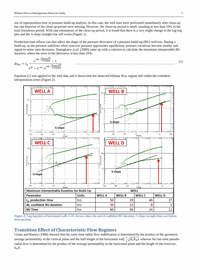
Production time effects can also affect the shape of the pressure derivative of a pressure build-up (BU) well test. During a
build-up, as the pressure stabilizes when reservoir pressure approaches equilibrium, pressure variations become smaller and
signal-to-noise ratio decreases. Daungkaew et al. (2000) came up with a criterion to calculate the maximum interpretable BU
duration, where the error in the derivative is less than 10%:
…………………………….………………………………………… (1)
Equation (1) was applied to the well data and it shows that the observed bilinear flow regime fall within the confident
interpretation zones (Figure 2).
Figure 2: Log-log plots of horizontal wells A-D. Arrows show the end of confident BU duration. ¼ slope straight-lines are before
these periods.
Transition Effect of Characteristic Flow Regimes Clonts and Ramey (1986) showed that the early-time radial flow stabilization is determined by the product of the geometric
average permeability in the vertical plane and the half-length of the horizontal well,
√ whereas the late-time pseudo-
radial flow is determined by the product of the average permeability in the horizontal plane and the height of the reservoir,
.

4 Bilinear Flow in Homogeneous Reservoir
Hence, it is possible that with certain combinations of vertical permeability anisotropy ratio, kV/kH, this could lead to a
transition effect from early-time radial flow stabilization to late-time pseudo-radial stabilization that may appear as a ¼ slope
straight line on the pressure derivative during intermediate-times.
A sensitivity analysis of the vertical permeability anisotropy ratio, kV/kH effect on the pressure derivative during intermediate-
times was performed on a homogeneous reservoir model based on computational methods detailed by Ozkan and Raghavan
(1991) integrated into the well test analysis software, Saphir (Ecrin 4.20.05) by KAPPA Engineering. It was found that with a
short effective well length, L of 500ft and a small kV/kH of 0.05, a quarter (¼) slope was observed in the pressure derivative.
However, the derivative slope quickly deviates away from ¼ when kV/kH decreases to 0.01 or increases to 0.1 (Figure 3). It is
also noted that the ¼ slope straight line in this case only appeared for duration of less than one log cycle whereas the observed
well test data extends up to two log cycles.
Figure 3: (Left) Sensitivity of kV/kH on transition effect from early-time radial flow stabilization to late-time pseudo-radial
stabilization. (Right) Sensitivity of zw/h to transition effect from early-time radial flow to hemiradial flow.
When the horizontal well is off-centered in the vertical plane, i.e. closer to either the top or bottom of the reservoir, hemiradial
flow is formed after early-time radial flow stabilization (Kuchuk et al., 1991). This will end when the flow reaches the
opposite boundary. In the case of a thin reservoir, the hemiradial flow stabilization lasts for a short period of time and then
transitions towards the linear flow, which may appear as a ¼ slope straight line straight line on the pressure derivative.
A sensitivity analysis of the distance to top boundary, zw as a function of the reservoir height, h was hence performed using the
Ozkan and Raghavan (1991) method (Figure 3). It was found that for this specific case at zw/h=0.33, a unique combination of
the transition effect from early-time radial flow stabilization to hemiradial flow stabilization; hemiradial flow stabilization to
linear flow and pseudo-radial flow stabilization resulted in a ¼ slope straight line lasting for approximately one and a half log-
cycle (1½).
Hence, it is shown here that ¼ slope straight line in the pressure derivative is not unique to bilinear flow but could be due to a
combination of the transition effects of the characteristic flow regimes in a horizontal well.
Comparing this to the well data, it is a plausible interpretation for well A but not for wells B, C and D (Figure 2) within the
constraints of the known well parameters. In wells B, C and D, the ¼ slope straight line in the pressure derivative starts earlier
and further investigation is required.
Numerical Simulation of Geological Effects Chen et al. (2012) suggested that the complexity of the depositional environment in turbidite reservoirs cannot be estimated
using conventional analytical models but can be captured by numerical simulation of the well test. In this study, a systematic
methodology for numerical simulation of the well test analysis was followed:
1. Gather input data for numerical model.
a. Verify reservoir connectivity with modified pulse tests.
b. Estimate areal anisotropy with existing well test data.
2. Build base case model in reservoir simulator (ECLIPSE100 version 2010.1 from Schlumberger).
a. Verify model behavior with existing examples in literature.

Bilinear Flow in Homogeneous Reservoir Study 5
3. Create numerical model of geological features.
4. Compare and analyze well test outputs from simulation to real well test data.
Input Data for Numerical Model Table 1: Input Parameters for Numerical Model used for all simulations.
Input Parameters Units Value Data Source
Porosity, ϕ - 0.20 Well logs
Maximum reservoir thickness, h ft 120 Well logs
Oil gravity °API 43 PVT Report
Oil viscosity, µ cP 0.3 PVT Report
Formation Volume Factor, B rb/stb 1.6 PVT Report
Gas Oil Ratio, GOR scf/stb 900 PVT Report
Bubble Point Pressure, Pb psi 2200 PVT Report
Total compressibility, ct 1/psi 2E-5 Calculated: ct = Soco+Swcw+cf
Initial Reservoir Pressure psi 4000 Huntington Field Development Report
Datum Depth ft 8600 Huntington Field Development Report
Reservoir Connectivity
Figure 4: Map of Huntington field and locations of wells. Wells V1 and V2 are vertical, Wells A, B, C and D are horizontal.
In order to establish reservoir-wide connectivity and discount any evidence of barrier effects on the well test analysis, modified
pulse tests had been performed, where a series of short production and shut-in periods were applied at the active well (during
clean-up and test) and the resulting pressure response recorded at the observation well. Three modified pulse tests were
performed in this reservoir:
Well A (Active Well) with Well C (Observation Well)
Well D (Active Well) with Well C (Observation Well)
Well B (Active Well) with Wells C and D (Observation Wells)
The results of the modified pulse tests indicate no obvious barriers between the wells and good reservoir connectivity between
all the wells (Appendix D). Further analysis of the modified pulse test data also show that the mismatch of porosity and
permeability values of the tests could potentially be due to varying reservoir thickness and porosity in the reservoir (Table 2).
Table 2: Modified Pulse Test Analysis Results as compared to Well Test Analysis
Estimated Permeability Wells B & C Wells B & D Wells D & C Wells A &C
Well k (mD) k (mD) k (mD) k (mD) k (mD)
A 39 - - - 34
B 54 25 25 - -
C 63 25 - 35 34
D 39 - 25 35 -
Porosity, ϕ 21% 7% 6% 5% 9%
Mid-Point distance between wells, ft 5,106 7,236 2,114 2,271
Time lag, hr 110 204 11 21

6 Bilinear Flow in Homogeneous Reservoir
Areal Anisotropy The modified pulse tests indicate possible reservoir heterogeneity between the wells. Based on the seismic impedance map of
the reservoir (Figure 5), it is shown that the channels typically lie in the NW-SE direction. If areal anisotropy exists in this
reservoir, the minimum permeability direction, kX should then lie perpendicular to this i.e. the NE-SW direction. In order to
verify this, an analytical solution published by Zhang and Dusseault (1996) were used, where the four possible roots of the
direction of the minimum permeability can be determined from sets of two horizontal and one vertical well tests.
The analytical solution is applied on the three pairs of horizontal wells (B & C, B & D and B & A). It is found that the results
agree with the seismic impedance map, where the minimum permeability direction, kX lies in the NE-SW direction i.e. azimuth
of 44°-61° & 224°-241° (Figure 5). It is also calculated that the permeability contrast between the maximum and minimum
horizontal permeability, kY/kX ranges from 2 – 15x (Appendix E: Table E-1).
Figure 5: (Left) Seismic impedance map overlaid with location map of wells showing general channel direction of NW-SE. (Right)
Two possible minimum permeability, kX direction, one lying approximately NW-SE and the other NE-SW (more likely geologically).
Base Model Construction and Verification Table 3: Model Dimensions
X Y Z TOTAL
Grid Size (ft) 17,208 49,153 100 8.46×1010 ft3
Grid Cells 72 39 9 25,272
In order to establish an efficient and accurate flow model, grid cells were logarithmically-spaced in the X, Y and Z direction.
Care was taken to ensure boundary effects were not encountered during the simulation. Therefore, the direction perpendicular
to the well, Y-direction stretches over a larger distance than the X-direction. Also, to ensure that the pressure changes are
accurately captured in the model, a fine grid is applied to the length of the well, leading to more cells in the X-direction of the
model. The dimensions of the base model are shown in Table 3.
Figure 6: (Left) Base model showing the logarithmically-spaced grids; vertical exaggeration 10x. (Right) Dimensionless log-log plot
comparing the simulation to analytical solutions by Odeh and Babu (1990) and Ozkan and Raghavan (1991).
Bilinear Flow in Homogeneous Reservoir Study 7
In order to validate the behavior of the base model, the simulation was compared to the analytical models by Odeh and Babu
(1990) and Ozkan and Raghavan (1991). A good match is found between the simulations with the model by Ozkan and
Raghavan (1991) but the Odeh and Babu (1990) solution does not account for the transition effect from linear flow to pseudo-
radial flow (Figure 6). Further validation of the model behavior to variations of well parameters is included in Appendix F.
Numerical Modeling of Geological Features and Comparison to Well Data Now that it is established that there are no barriers between the horizontal wells from the modified pulse tests and possible
areal anisotropy, plausible geological features in the reservoir that may lead to a bilinear flow regime can be modeled. In
turbidite reservoirs, the degree of amalgamation, dimensions of lobe size, channel width, flow barriers in the form of cemented
gravel lags or shale drapes and their coverage may affect well test data (Chen et al., 2012). The following geological features
were modeled and its pressure behavior analyzed:
Horizontal well intersecting a high-permeability streak,
Dual layer formation with higher-permeability layer overlying lower-permeability layer,
Laterally extensive low-permeability thin layer underlying horizontal well, and
Multi-layered formation with varying vertical permeability.
In all cases, a similar well profile and well parameters which approximates the well data were used. Unless mentioned
otherwise, all the following models are for a horizontal well length, L of 3000ft, an average horizontal permeability, kH of
50mD and a total reservoir thickness, h of 120ft. All models use the input data as specified in Table 1.
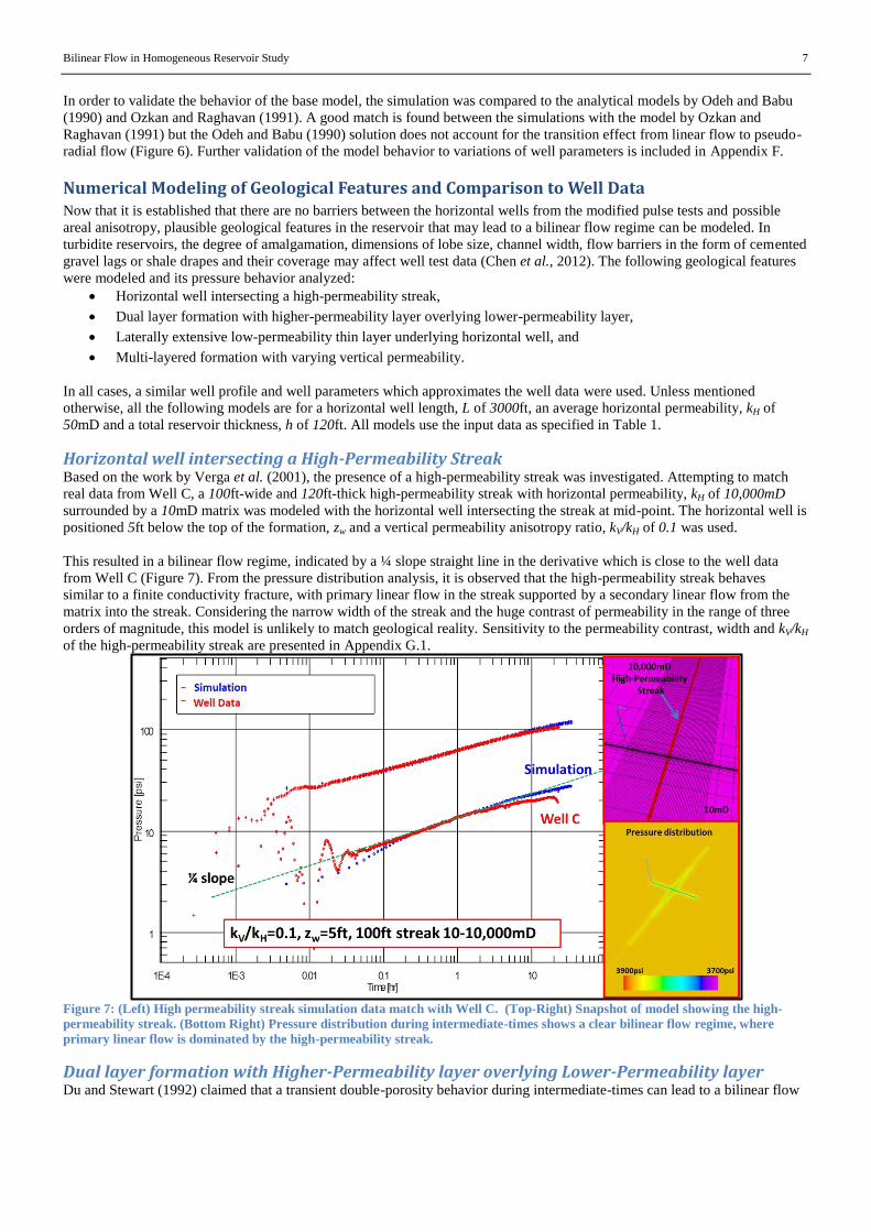
Horizontal well intersecting a High-Permeability Streak Based on the work by Verga et al. (2001), the presence of a high-permeability streak was investigated. Attempting to match
real data from Well C, a 100ft-wide and 120ft-thick high-permeability streak with horizontal permeability, kH of 10,000mD
surrounded by a 10mD matrix was modeled with the horizontal well intersecting the streak at mid-point. The horizontal well is
positioned 5ft below the top of the formation, zw and a vertical permeability anisotropy ratio, kV/kH of 0.1 was used.
This resulted in a bilinear flow regime, indicated by a ¼ slope straight line in the derivative which is close to the well data
from Well C (Figure 7). From the pressure distribution analysis, it is observed that the high-permeability streak behaves
similar to a finite conductivity fracture, with primary linear flow in the streak supported by a secondary linear flow from the
matrix into the streak. Considering the narrow width of the streak and the huge contrast of permeability in the range of three
orders of magnitude, this model is unlikely to match geological reality. Sensitivity to the permeability contrast, width and kV/kH
of the high-permeability streak are presented in Appendix G.1.
Figure 7: (Left) High permeability streak simulation data match with Well C. (Top-Right) Snapshot of model showing the high-
permeability streak. (Bottom Right) Pressure distribution during intermediate-times shows a clear bilinear flow regime, where
primary linear flow is dominated by the high-permeability streak.
Dual layer formation with Higher-Permeability layer overlying Lower-Permeability layer Du and Stewart (1992) claimed that a transient double-porosity behavior during intermediate-times can lead to a bilinear flow

8 Bilinear Flow in Homogeneous Reservoir
regime. For a horizontal well within a higher-permeability layer overlying a lower-permeability layer, this is analogous to a
dual-porosity system where two regions of different storativity and mobility exist. Since the porosity is the same in both layers,
the storativity in this case refers to the thickness of the 2 layers. The bilinear flow regime exists when the region of high
mobility (thin high-permeability layer) carries the reservoir fluid into the horizontal well while being fed by the region with
high storativity (thick low-permeability layer).
A reasonable match was found with a two-layer model consisting of a high-permeability 15ft thick layer with horizontal
permeability, kH of 250mD and a lower-permeability 105ft thick layer with kH of 25mD. The horizontal well is positioned 7.5ft
below the top of the formation, zw. The vertical permeability anisotropy ratio, kV/kH was matched at 0.03. A clear ¼ slope
straight line stretching over one log cycle is shown developing during intermediate-time (Figure 8).
Figure 8: Two-layer transient double porosity behavior simulation match with well data. (Inset) Graphical representation of
dimensions and well parameters used in the simulation model.
In order for a two-layer structure of different horizontal permeabilities, kH to exist in the formation, there has to be a clear
distinction in terms of porosity and/or grain sorting in the formation resulting in permeability contrast of more than one order
of magnitude. Correlating with the geological study, petrophysical evidence from well logs and core data, there is no
indication of a high horizontal permeability, kH contrast two-layer structure in the Huntington field. Sensitivity to the
permeability contrast, thickness and kV/kH of the 2-layer model are presented in Appendix G.2.
Laterally extensive Low-Permeability thin layer underlying Horizontal Well
Figure 9: Simulation data match with well data, where a low permeability thin layer is underlying a horizontal well. (Inset)
Graphical representation of dimensions and well parameters used in the simulation model.
Bilinear Flow in Homogeneous Reservoir Study 9
Based on the work by Briceño et al. (2002), it was reported that a bilinear flow regime is observed in well tests for horizontal
wells that are overlying or underlying formations with a shale barrier. This was attributed to the transient double porosity
behavior as explained by Du and Stewart (1992) above.
Applying the concept to this study to match the well data, a ¼ slope straight line lasting close to one log cycle was found in the
pressure derivative with a laterally extensive low-permeability 1ft thin layer of horizontal permeability, kH of 1mD and vertical
permeability, kV of 0.1mD (Figure 9). This thin low-permeability layer has an overlying 40ft thick and underlying 80ft thick
layer of horizontal permeability, kH of 50mD and vertical permeability, kV of 5mD.
Varying the vertical permeability, kV and thicknesses of the individual layers does not extend the ¼ slope straight line further
(Appendix G.3). Geological study of analogues and the core data of vertical wells also do not provide any evidence for the
existence of laterally extensive shale barriers in the Huntington field.
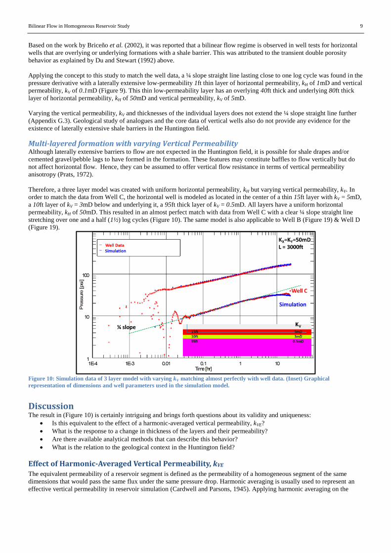
Multi-layered formation with varying Vertical Permeability Although laterally extensive barriers to flow are not expected in the Huntington field, it is possible for shale drapes and/or
cemented gravel/pebble lags to have formed in the formation. These features may constitute baffles to flow vertically but do
not affect horizontal flow. Hence, they can be assumed to offer vertical flow resistance in terms of vertical permeability
anisotropy (Prats, 1972).
Therefore, a three layer model was created with uniform horizontal permeability, kH but varying vertical permeability, kV. In
order to match the data from Well C, the horizontal well is modeled as located in the center of a thin 15ft layer with kV = 5mD,
a 10ft layer of kV = 3mD below and underlying it, a 95ft thick layer of kV = 0.5mD. All layers have a uniform horizontal
permeability, kH of 50mD. This resulted in an almost perfect match with data from Well C with a clear ¼ slope straight line
stretching over one and a half (1½) log cycles (Figure 10). The same model is also applicable to Well B (Figure 19) & Well D
(Figure 19).
Figure 10: Simulation data of 3 layer model with varying kV matching almost perfectly with well data. (Inset) Graphical
representation of dimensions and well parameters used in the simulation model.
Discussion The result in (Figure 10) is certainly intriguing and brings forth questions about its validity and uniqueness:
Is this equivalent to the effect of a harmonic-averaged vertical permeability, kVE?
What is the response to a change in thickness of the layers and their permeability?
Are there available analytical methods that can describe this behavior?
What is the relation to the geological context in the Huntington field?
Effect of Harmonic-Averaged Vertical Permeability, kVE The equivalent permeability of a reservoir segment is defined as the permeability of a homogeneous segment of the same
dimensions that would pass the same flux under the same pressure drop. Harmonic averaging is usually used to represent an
effective vertical permeability in reservoir simulation (Cardwell and Parsons, 1945). Applying harmonic averaging on the

10 Bilinear Flow in Homogeneous Reservoir
vertical permeabilities of the 3-layer model in (Figure 10) resulted in kVE = 0.61mD (Appendix I: Equation (H- 3)).
Figure 11: Log-log plot of 1-layer model with equivalent vertical permeability, kVE (Left) and 3-layer varying kV model. (Right)
Keeping all other well parameters the same, the harmonic-averaged vertical permeability was then used to model an equivalent
single-layer model which was then compared to the 3-layer model (Figure 11). It is observed that the harmonic averaged
model also produces a ¼ slope straight line but with a shorter duration of less than 1 log cycle at intermediate-times. In the 3-
layer uniform kH but varying kV model, the early-time flow stabilization is not present and pseudo-radial flow stabilization
begins later.
Sensitivity to Layer Thickness and Permeability The sensitivity to the layer thickness of the top layer (L1) in the 3-layer uniform kH but varying kV model and the permeability
of middle layer (L2) were also modeled. The results show that the ¼ slope straight line is very sensitive to small changes in
either the L1 thickness or L2 permeability (Figure 12). It is also found that the derivative is less sensitive to changes in the
middle layer (L2), bottom layer (L3) thickness and L1, L3 vertical permeability, kV. (Appendix G.4)
Figure 12: (Left) Sensitivity to L1 thickness. (Right) Sensitivity to L2 permeability.
In the earlier section, it was pointed out that there could be a possibility of the presence of areal anisotropy. Modifying the 3-
layered model with uniform kH but varying kV to one with areal permeability anisotropy ratio, kY/kX = 5; a good match with
well C was also achievable. However, this is at the expense of halving the average horizontal permeability, kH to 25mD
(Figure 13). Vertical well tests however show an average horizontal permeability, kH of 40-55mD.
It is also shown that the model behavior is insensitive to the thickness of the least permeable layer, L3 (Appendix G.4: Figure
G-14). A model with 4 layers of varying kV also provided a match with well data (Figure 14). The horizontal well is modeled
to be in the center of a thin 15ft layer with kV = 5mD, a 10ft layer of kV = 3mD below, a 55ft layer of kV = 0.5mD underlying it
and finally a 40ft layer of kV = 5mD at the bottom. All layers have a uniform kH of 50mD.

Bilinear Flow in Homogeneous Reservoir Study 11
Figure 13: Simulation data of 3 layer model with varying kV and kY/kX = 5 matching almost perfectly with well data. (Inset)
Graphical representation of dimensions and well parameters used in the simulation model.
Figure 14: Simulation data of 4 layer model with varying kV matching almost perfectly with well data. (Inset) Graphical
representation of dimensions and well parameters used in the simulation model.
Analytical Solution to Bilinear Flow Regime A streamline simulation was created to understand the flow regime during intermediate-times better. It is shown that bilinear
flow regime indeed happened during intermediate-times for the 3-layer varying kV model (Figure 15).
Two straight-line analytical solutions of √
was found to provide a close estimation of the well parameters:
Finite-Conductivity Fracture Model
Transient Double-Porosity Model
Finite-Conductivity Fracture Model
( ) ( )
………………………..…………………………….…………………… (2)
12 Bilinear Flow in Homogeneous Reservoir
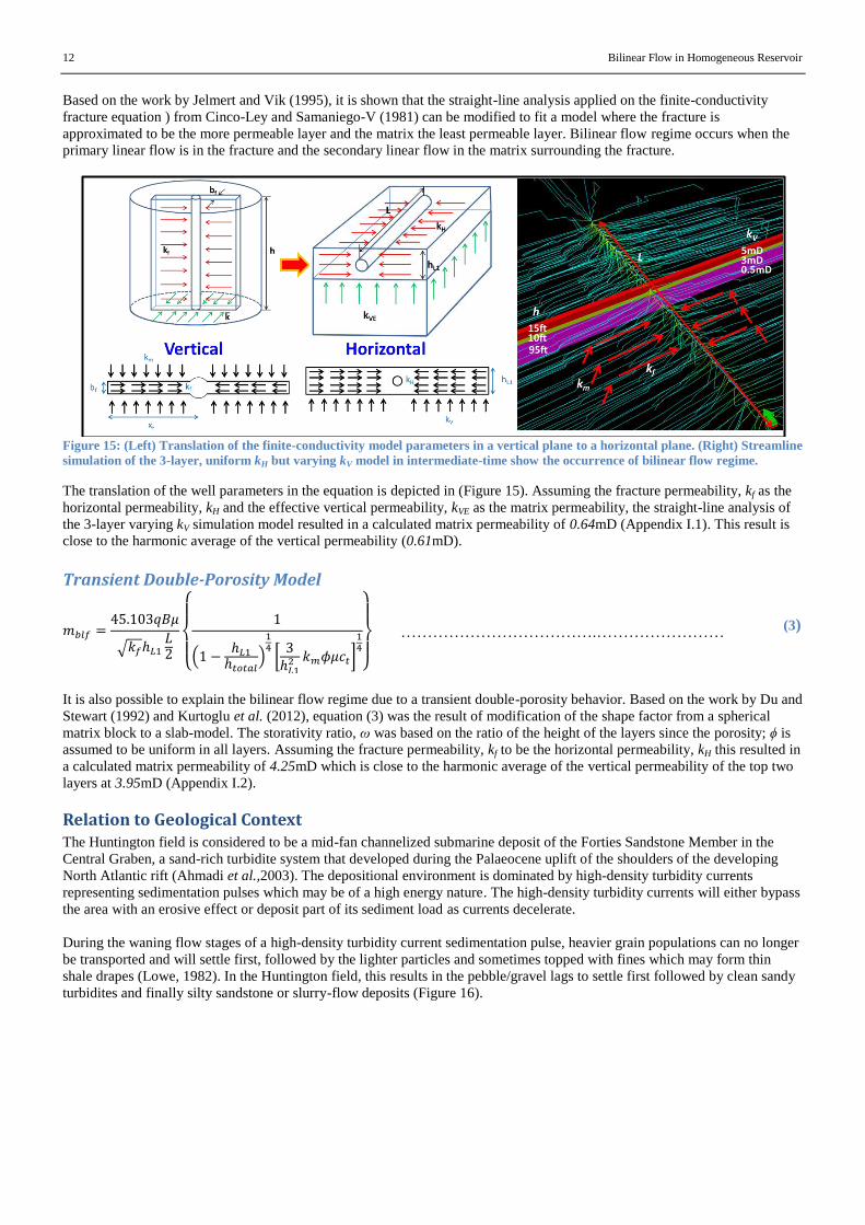
Based on the work by Jelmert and Vik (1995), it is shown that the straight-line analysis applied on the finite-conductivity
fracture equation ) from Cinco-Ley and Samaniego-V (1981) can be modified to fit a model where the fracture is
approximated to be the more permeable layer and the matrix the least permeable layer. Bilinear flow regime occurs when the
primary linear flow is in the fracture and the secondary linear flow in the matrix surrounding the fracture.
Figure 15: (Left) Translation of the finite-conductivity model parameters in a vertical plane to a horizontal plane. (Right) Streamline
simulation of the 3-layer, uniform kH but varying kV model in intermediate-time show the occurrence of bilinear flow regime.
The translation of the well parameters in the equation is depicted in (Figure 15). Assuming the fracture permeability, kf as the
horizontal permeability, kH and the effective vertical permeability, kVE as the matrix permeability, the straight-line analysis of
the 3-layer varying kV simulation model resulted in a calculated matrix permeability of 0.64mD (Appendix I.1). This result is
close to the harmonic average of the vertical permeability (0.61mD).
Transient Double-Porosity Model
√
{
(
)
[
]
}
……………………………….…………………… (3)
It is also possible to explain the bilinear flow regime due to a transient double-porosity behavior. Based on the work by Du and
Stewart (1992) and Kurtoglu et al. (2012), equation (3) was the result of modification of the shape factor from a spherical
matrix block to a slab-model. The storativity ratio, ω was based on the ratio of the height of the layers since the porosity; ϕ is
assumed to be uniform in all layers. Assuming the fracture permeability, kf to be the horizontal permeability, kH this resulted in
a calculated matrix permeability of 4.25mD which is close to the harmonic average of the vertical permeability of the top two
layers at 3.95mD (Appendix I.2).
Relation to Geological Context The Huntington field is considered to be a mid-fan channelized submarine deposit of the Forties Sandstone Member in the
Central Graben, a sand-rich turbidite system that developed during the Palaeocene uplift of the shoulders of the developing
North Atlantic rift (Ahmadi et al.,2003). The depositional environment is dominated by high-density turbidity currents
representing sedimentation pulses which may be of a high energy nature. The high-density turbidity currents will either bypass
the area with an erosive effect or deposit part of its sediment load as currents decelerate.
During the waning flow stages of a high-density turbidity current sedimentation pulse, heavier grain populations can no longer
be transported and will settle first, followed by the lighter particles and sometimes topped with fines which may form thin
shale drapes (Lowe, 1982). In the Huntington field, this results in the pebble/gravel lags to settle first followed by clean sandy
turbidites and finally silty sandstone or slurry-flow deposits (Figure 16).

Bilinear Flow in Homogeneous Reservoir Study 13
Figure 16: (Top Left) Diagram showing the characteristics of a high-density turbidite current that dominates the depositional
environment in the Huntington field (Haughton et al., 2009). (Bottom Left) Diagram pointing to a mid-fan channelized submarine
deposit which characterizes the Huntington field (SEPM STRATA, 2013). (Right) Photographs of core samples from the bottom to
top of reservoir showing the coarse to fine transition. Arrows point to pebbles present in the reservoir.
Figure 17: Core description chart of well V1 (Left) and V2 (Right), Scale 1:200MD.

14 Bilinear Flow in Homogeneous Reservoir
The presence of strongly varying vertical permeability and uniform horizontal permeability could in specific cases be
explained by the presence of cemented pebble/gravel lags which sometimes occur at the base of channel deposits due to the
process of diagenesis or by thin shale drapes formed by the settlement of the silt and clay particles during waning flow
conditions at the final stage of a sedimentation pulse. These features are however non-uniform and not laterally extensive.
Hence, they will form local baffles rather than barriers to vertical flow and do not normally obstruct horizontal flow.
Core data from two near-vertical wells, V1 and V2 (Figure 4), show good agreement with the well test data of closely located
horizontal wells A and C (Figure 17). The core of V2 near well A show very clean sand deposits with a high percentage of
sand and low percentage of clay, silt and pebble/gravel lag. This is in agreement with well test data from well A which can be
approximated by a homogeneous model (Figure 18).
Figure 18: Matching of the simulation results of homogeneous model with well A.
In comparison, core of V1 also shows a high percentage of sand but lower than V2. Most importantly, there is a higher
percentage of clay, silt and pebble lag compared to well V2. In the core log of V1 (Figure 17), there appear to be three distinct
depositional sequences:
Sequence I consists of clean; moderately to well sorted fine grained sandstone.
Sequence II consists of moderately well sorted sandstone with occasional swelling, angular mudclasts.
Sequence III consists of pebbly sandstones and locally pervasive calcite cement.
This seem to relate well with the multi-layer varying vertical permeability, kV model that matches well test data from wells B
(Figure 19), C (Figure 10) and D (Figure 19).
Figure 19: (Left) Matching of the simulation results of a 3-layer uniform kH but varying kV model with well B. (Right) Matching of
the simulation results of a 2-layer uniform kH but varying kV model with well D.
Conclusion The approach presented in this study successfully identified the plausible models for bilinear flow regime in the Huntington
field. As a result of this study, the following observations and conclusions were reached:

Bilinear Flow in Homogeneous Reservoir Study 15
Quarter (¼) slope in the derivative is non-unique to bilinear flow regimes and could be achieved due to the transition
effect between flow regimes in a horizontal well.
Bilinear flow regimes can occur in the following cases:
o Horizontal well intersecting a narrow high permeability streak, approximating a finite conductivity fracture.
o Dual-layer formation with higher permeability layer containing horizontal well overlying layer with
permeability one order of magnitude lower due to transient double-porosity behavior.
o Laterally extensive thin low-permeability layer underlying a horizontal well also due to transient double-
porosity behavior.
o Multi-layered formation of uniform horizontal permeability, kH but varying vertical permeability, kV with the
horizontal well within the higher kV layer overlying layers of progressively lower kV.
The Huntington field well test data suggests the multi-layered formation of uniform horizontal permeability, kH but
on-uniform vertical permeability, kV is the closest match to wells B (Figure 19), C (Figure 10) and D (Figure 19),
whereas Well A matches a homogeneous reservoir model (Figure 18).
The presence of strongly varying kV and uniform kH could be explained by the cemented pebble/gravel lags which
occur at the base of channel deposits or by thin shale drapes formed by the settlement of silt and clay particles during
waning flow conditions at the final stages of a high-density turbidity current sedimentation pulse. As these features
are non-uniform and not laterally extensive, they form local baffles to vertical flow but do not obstruct horizontal
flow.
Straight-line analytical solutions based on the finite conductivity model (Cinco-Ley and Samaniego-V, 1981) or the
transient double porosity model (Kurtoglu et al., 2012) can give an approximate averaged equivalent vertical
permeability, kVE solution.
Suggestions for Further Work The presence of vertical baffles to flow in the multi-layered varying vertical permeability model may be of concern as Jackson
and Muggeridge (1999) have shown that inclined and intersecting discontinuous shales on horizontal waterfloods may alter the
sweep efficiency. Integration of the findings in this study into the full-field model for the Huntington field could potentially
provide a better understanding of the reservoir dynamics and flow behavior. This could lead to better prediction and
optimization of the reservoir performance.
As it stands, the well tests data were performed right after completion and clean-up. If further well test data is available in
conjunction with production data, deconvolution can be applied to further understand the behavior of the pressure derivative in
the reservoir.
Finally, as the straight-line analytical solutions are insufficient to accurately predict the vertical permeability, kV in each
individual layer of the multi-layer varying kV model, further study is required to come up with a new analytical solution for this
model. Suzuki and Nanba (1991) published an analytical solution for stratified reservoirs by approximating stratified reservoir
behavior to horizontal well single layer solution. However, as pointed out by the author, this method is unsuitable when the
vertical permeability, kV of the layers is extremely low, where the resulting linear flow would only reflect the properties of the
sublayer containing the horizontal well.
Nomenclature ΔtBU confident build-up duration (hrs)
µ viscosity (cP)
ϕ porosity
σ shape factor
ω storativity ratio
Anoise amplitude of noise (psi)
B formation volume factor (rb/stb)
bf fracture width (ft)
cf compressibility of formation (1/psi)
co compressibility of oil (1/psi)
ct total compressibility (1/psi)
cw compressibility of water (1/psi)
h reservoir thickness (ft)
k permeability (mD)
kf fracture permeability (mD)
kH average horizontal permeability (mD)
km matrix permeability (mD)
kV vertical permeability (mD)
kVE equivalent vertical permeability (mD)
kX minimum horizontal permeability (mD)
kY maximum horizontal permeability (mD)
L effective horizontal well length (ft)
mblf slope of straight-line in plot of √
pD dimensionless pressure
q oil flow-rate (stb/d)
So oil saturation
Sw water saturation
tD dimensionless time
tP production time (hrs)
W window half-length
zw horizontal well vertical distance to top (ft)

16 Bilinear Flow in Homogeneous Reservoir
References Ahmadi, Z., Kenyon-Roberts, M., Stanworth, S., Kugler, C., Kristensen, K., & Fugelli, E. (2003). Palaeocene. In D. Evans, C.
Graham, C. Armour, & P. Bathurst (Eds.), The Millennium Atlas: Petroleum Geology of the Central and Northern
North Sea (pp. 235-260). Geological Society of London.
Baba, A., Azzouguen, A., Mazouzi, A., Tiab, D., & Aissaoui, K. (2002). Determination of the Controlling Factors and Origins
of the Bilinear Flow from Horizontal Well Transient Responses. 2002-018 Petroleum Society CIMMP, presented at
Canadian International Petroleum Conference, Calgary, 11-13 June.
Briceño, M., Summers, L., & Quijada, O. (2002). Horizontal Wells Pressure Build Up Analysis in Orinoco Heavy Oil Belt.
SPE78969, presented at SPE ITOHOS, Calgary, 4-7 November.
Cardwell, W., & Parsons, R. (1945). Average Permeabilities of Heterogeneous Oil Sands. SPE945034, Transactions of the
AIME, 160(1), 34-42.
Chen, T., Noirot, J., Khandelwal, A., Xue, G., Barton, M., & Alpak, F. (2012). Estimating Stratigraphic Parameters from Well
Test Data in Turbidite Reservoirs. SPE159090, presented at SPE ATCE, San Antonio, 8-10 October.
Cinco-Ley, H., & Samaniego-V, F. (1981). Transient Pressure Analysis for Fractured Wells. SPE7490, Journal of Petroleum
Technology, September, 1749-1766.
Clonts, M., & Ramey, H. (1986). Pressure Transient Analysis for Wells with Horizontal Drainholes. SPE15116 presented at
SPE California Regional Meeting, Oakland, 2-4 April.
Daungkaew, S., Hollaender, F., & Gringarten, A. (2000). Frequently Asked Questions in Well Test Analysis. SPE63077,
presented at SPE ATCE, Dallas, 1-4 October.
Daviau, F., Mouronval, G., Bourdarot, G., & Curutchet, P. (1988). Pressure Analysis for Horizontal Wells. SPE14251, SPE
Formation Evaluation, 716-724.
Du, K., & Stewart, G. (1992). Transient Pressure Response of Horizontal Wells in Layered and Naturally Fractured Reservoirs
with Dual-Porosity Behavior. SPE24682, presented at 67th SPE ATCE, Washington, 4-7 October.
Goode, P., & Thambynayagam, R. (1987). Pressure Drawdown and Buildup Analysis of Horizontal Wells in Anisotropic
Media. SPE14250, SPE Formation Evaluation, 683-697.
Haughton, P., Davis, C., McCaffrey, W., & Barker, S. (2009). Hybrid sediment gravity flow deposits - Classification, origin
and significance. Marine and Petroleum Geology(26), 1900-1918.
Jackson, M., & Muggeridge, A. (1999). Effect of Discontinuous Shales on Reservoir Performance during Horizontal
Waterflooding. SPE69751, presented at SPE Reservoir Simulation Symposium, Houston, 14-17 February.
Jelmert, T. (2000). Horizontal wells provide bilinear pressure signatures. Oil & Gas Journal, Volume 98(Issue 46).
Jelmert, T., & Vik, S. (1995). Producing Horizontal Wells Bilinear flow may occur in horizontal wells. Oil & Gas Journal,
Volume 93(Issue 50).
Kuchuk, F., Goode, P., Wilkinson, D., & Thambynayagam, R. (1991). Pressure-Transient Behavior of Horizontal Wells With
and Without Gas Cap or Aquifer. SPE17413, SPE Formation Evaluation, 86-94.
Kurtoglu, B., Torcuk, M., & Kazemi, H. (2012). Pressure Transient Analysis of Short and Long Duration Well Tests in
Unconventional Reservoirs. SPE162473, presented at SPE CURC, Calgary, 30 October - 1 November.
Lowe, D. (1982). Sediment Gravity Flows: II. Depositional Models with Special Reference to the Deposits of High-Density
Turbidity Currents. Journal of Sedimentary Petrology, 52(1), 279-297.
Nurafza, P., Diepeveen, P., & Arkley, P. (2013). Huntington Development Well Tests Report; E.ON UK Ltd Internal Report.
Odeh, A., & Babu, D. (1990). Transient Flow Behavior of Horizontal Wells: Pressure Drawdown and Buildup Analysis.
SPE18802, SPE Formation Evaluation, 7-15.
Ozkan, E., & Raghavan, R. (1991). New Solutions for Well-Test-Analysis Problems: Part 1 - Analytical Considerations & Part
2 - Computational Considerations and Applications. SPE18616, SPE Formation Evaluation, 359-378.
Ozkan, E., Raghavan, R., & Joshi, S. (1989). Horizontal-Well Pressure Analysis. SPE16378, SPE Formation Evaluation, 567-
575.
Prats, M. (1972). The Influence of Oriented Arrays of Thin Impermeable Shale Lenses or of Highly Conductive Natural
Fractures on Apparent Permeability Anisotropy. SPE4163, Journal of Petroleum Technology (JPT) Forum, October,
1219-1221.
SEPM STRATA. (2013, February 15). SEPM Stratigraphy Web - Ross Formation - Upper Carboniferous Deepwater
Sediments. Retrieved August 23, 2013, from http://www.sepmstrata.org/page.aspx?pageid=259
Suzuki, K., & Nanba, T. (1991). Horizontal Well Pressure Transient Behavior in Stratified Reservoirs. SPE22732, presented at
66th SPE ATCE in Dallas, 6-9 October.
Verga, F., Beretta, E., & Albani, D. (2001). Transient Dual-Porosity Behavior for Horizontal Wells Draining Heterogeneous
Reservoirs. SPE68844, presented at SPE Western Regional Meeting, Bakersfield, 26-30 March.
Zhang, L., & Dusseault, M. (1996). Anisotropic Permeability Estimation by Horizontal Well Tests. SPE37071, presented at
SPE ICHWT in Calgary, 18-20 November.

Bilinear Flow in Homogeneous Reservoir Study 17
Appendix A: Critical Milestones
Source Year Title Authors Contribution
SPE7490 1981 Transient Pressure Analysis
for Fractured Wells
H. Cinco-Ley First to introduce concept of bilinear flow
that yields a straight line on a plot of
√
. F. Samaniego-V
SPE15116 1986
Pressure Transient Analysis
for Wells with Horizontal
Drain Hole
M.D. Clonts First to analyze transient pressure behavior
of horizontal drainholes compared to
vertical fractures and defined horizontal
well characteristic flow regimes. H.J. Ramey Jr.
SPE17413 1991
Pressure Transient Behavior
of Horizontal Wells with
Gascap or Aquifer
F.J. Kuchuk
Introduced concept of hemiradial flow
when horizontal well is off-centered in the
vertical plane of a reservoir.
SPE18616 1991
New Solutions for Well-
Test-Analysis Problems: Part
1 & Part 2.
E. Ozkan Provided computational framework for
analytical solution of horizontal wells using
Bessel functions which can then be solved
using the Stehfest algorithm. R. Raghavan
SPE24682 1992
Transient Pressure Response
of Horizontal Wells in
Layered and Naturally
Fractured Reservoirs with
Dual Porosity Behavior
K.F. Du First to show how bilinear flow can arise in
the case of a horizontal well in a transient
“dual porosity” (fractured or layered)
reservoir. O. Stewart
Oil & Gas
Journal,
Volume 93,
Issue 50
1994
Producing Horizontal Wells
Bilinear Flow may occur in
Horizontal Wells
T.A. Jelmert First to show bilinear flow may occur in
homogeneous reservoirs with horizontal
wells, from linear flow opposite long
horizontal section and flow from areas
beyond the well tips.
S.A. Vik
SPE68844 2001
Transient Dual-Porosity
Behavior for Horizontal
Wells Draining
Heterogeneous Reservoirs
F.M. Verga Exhibited case of bilinear flow when
horizontal well intersects a vertical high-
permeable zone surrounded by a lower
permeability zone.
E. Beretta
D. Albani
SPE78969 2002
Horizontal Wells Pressure
Build Up Analysis in
Orinoco Heavy Belt
M. Briceño Bilinear flow observed when horizontal
well intersects compound sands consisting
of multiple parasequences (amalgated or
separated by shale barriers)
L.E. Summers
O.J. Qujida
Geological
Society of
London
Publication
2003
Chapter 14, Palaeocene; The
Millennium Atlas: Petroleum
Geology of the Central and
Northern North Sea
Z.M. Ahmadi Characterized the stratigraphy and
sedimentology of the Palaeocene
sandstones in submarine fans within the
Central North Sea where the Huntington
field is located.
M. Kenyon-Roberts
S. Stanworth
C.W. Kugler
K.A. Kristensen
E.M.G. Fugelli
SPE159090 2012
Estimating Stratigraphic
Parameters from Well Test
Data in Turbidite Reservoirs
T. Chen Demonstrated effect of shale drape
coverage in reservoir well test analysis of
turbidite reservoirs. Channel shale drape
coverage of 0.40 approximate bilinear flow
regimes.
J. Noirot
A. Khandelwal
G. Xue
M.D. Barton
F.O. Alpak
SPE162473 2012
Pressure Transient Analyses
of Short and Long Duration
Well Tests in
Unconventional Reservoirs
B. Kurtoglu Modified the work by Du and Stewart
(1992), for an analytical solution for
transient double-porosity behavior in a
horizontal well.
M.A. Torcuk
H.Kazemi

18 Bilinear Flow in Homogeneous Reservoir
Appendix B: Critical Literature Review
SPE 7490 (1981)
Title: Transient Pressure Analysis for Fractured Wells
Authors: H. Cinco-Ley, F. Samaniego-V
Contribution: First to introduce concept of bilinear flow that yields a straight line on a plot of √
for finite
conductivity vertical fracture.
Objective of Paper: Present new interpretation technique for early-time pressure data of a well intercepted by a finite-
conductivity vertical fracture.
Methodology used: Assuming small pressure gradients, negligible gravity effects and flow entering wellbore comes only
through the fracture; the diffusivity equation is used to describe the unsteady state flow in the system.
Conclusion reached: Bilinear flow occurs when 2 linear flows occur simultaneously. One flow is a linear incompressible flow
within the fracture and the other is a linear compressible flow in the formation. Bilinear flow exists whenever most of the fluid
entering the wellbore comes from the formation and fracture tip effects has not yet affected the well behavior. The paper also
presented new technique and type curves to analyze data in bilinear flow period.
Comments: This paper introduces the concept of bilinear flow and provides an equation for the slope of a straight-line in a
plot of √
.

Bilinear Flow in Homogeneous Reservoir Study 19
SPE 15116 (1986)
Title: Pressure Transient Analysis for Wells with Horizontal Drain Hole
Authors: M.D. Clonts, H.J. Ramey Jr.
Contribution: First to analyze transient pressure behavior of horizontal drainholes compared to vertical fractures.
Objective of Paper: Present a method to understand horizontal drainholes using pressure transient analysis.
Methodology used: Derive solution to pressure transient response of horizontal drainholes using instantaneous source
functions together with the Newman product method.
Conclusion reached: Two possible types of transient pressure behavior were identified depending on effective dimensionless
drainhole half-length,
√
.
LD = dimensionless drainhole half-length
m = no. of drainholes in reservoir
xf = drainhole or fracture half-length
h = reservoir height
ki = permeability in i-direction.
If LD < 10, flow is characterized by an initial radial flow perpendicular to drainhole axis followed by transition to pseudo-
radial flow period. If LD > 10, initial radial flow period ends instantaneously. Flow is then characterized by early time linear
flow followed by a transition to late-time pseudo-radial flow.
Comments: First to define the early-time radial flow and late-time pseudo-radial flow stabilization flow regimes in horizontal
wells. This is later expanded by Goode and Thambynayagam (1987), Daviau et al. (1988), Ozkan et al. (1989), Odeh and
Babu (1990) and Kuchuk et al. (1991) to include analytical solutions for the intermediate-time linear flow regime solved using
source functions and Green’s function or Laplace and Fourier transforms.

20 Bilinear Flow in Homogeneous Reservoir
SPE 17413 (1991)
Title: Pressure Transient Behavior of Horizontal Wells with Gascap or Aquifer
Authors: F.J. Kuchuck
Contribution: Introduced concept of hemiradial flow when horizontal well is off-centered in the vertical plane of a reservoir.
Objective of Paper: Present a solution for transient pressure behavior for horizontal wells based on pressure-averaging
technique taking into consideration presence of constant pressure boundaries (gascap/aquifer).
Methodology used: Using uniform-flux line-source solution, the equation was solved in the Laplace-domain. Estimation of
pressure response at the well was performed by averaging the pressure along the well length rather than an equivalent pressure
point.
Conclusion reached: New solutions that can be applied to drawdown and buildup tests from horizontal wells with and
without a constant-pressure boundary (aquifer/gas cap) were derived for efficient computer implementation of the solutions.
Due to the large number of parameters involved, it is recommended to use non-linear least-squares estimation methods for
type-curve matching.
Comments: It is shown in this study that it is possible for ¼ slope straight line to appear due to unique combination of well
parameters that led to transition effects from early-time radial flow stabilization to hemiradial flow; hemiradial flow to linear
flow and pseudo-radial flow stabilization.

Bilinear Flow in Homogeneous Reservoir Study 21
SPE 18616 (1991)
Title: New Solution for Well-Test-Analysis Problems – Part 1: Analytical Considerations & Part 2: Computational
Considerations and Applications.
Authors: E. Ozkan and R. Raghavan
Contribution: Provided computational framework for analytical solution of horizontal wells.
Objective of Paper: Present procedures for computing well responses of vertically fractured well and horizontal well in
homogeneous or naturally fractured reservoirs.
Methodology used: Convert Laplace transformations of the analytical solutions for the well responses in terms of Bessel
functions so that it can be solved using the Stehfest algorithm.
Conclusion reached: Wide variety of complex problems of interest in well test analysis can be solved by exploiting the
advantages of the Laplace-transformation techniques.
Comments: This is integrated into the horizontal well analytical solutions of well test analysis software, Saphir (Ecrin
4.20.05) of Kappa Engineering which is used for sensitivity analysis of the transition effects of the characteristic flow regimes
in horizontal wells.

22 Bilinear Flow in Homogeneous Reservoir
SPE 24682 (1992)
Title: Transient Pressure Response of Horizontal Wells in Layered and Naturally Fractured Reservoirs with Dual Porosity
Behavior
Authors: K.F. Du, O. Stewart
Contribution: First to show how bilinear flow can arise in the case of a horizontal well in a transient “dual porosity”
(fractured or layered) reservoir.
Objective of Paper: Attribute the case of bilinear flow observed in horizontal wells to the presence of transient dual-porosity
behavior in the reservoir caused by:
Multi-layered reservoir
Naturally-fractured reservoir
Fracture Face (Interporosity) Skin
Areal anisotropy
Methodology used: Using the analytical solution for a uniform flux, line-source well in an anisotropic medium; a full
analytical solution is derived for the dual-porosity system. Aguilera’s method was used to substitute the storage-term in
homogeneous reservoir solution with a term involving storativity ratio.
Conclusion reached: Bilinear flow exhibited can be attributed to the dual porosity transition which can occur at any of the 3
flow regimes present in a horizontal well: radial vertical flow, linear flow opposite completed section and pseudoradial flow at
late time, depending on the value of the interporosity flow coefficient, λL. The smaller λL is, the later the dual porosity effect
occurs.
For the layered system, 2 linear flow will occur if the horizontal well lies in a high permeability layer (linear horizontal)
supported by a tight zone (linear vertical), resulting in a bilinear flow due to the averaging of the 2 linear flows.
Comments: This paper supports a plausible interpretation for the bilinear flow observed in this case study. The analytical
solution is re-derived later by Kurtoglu et al. (2012).
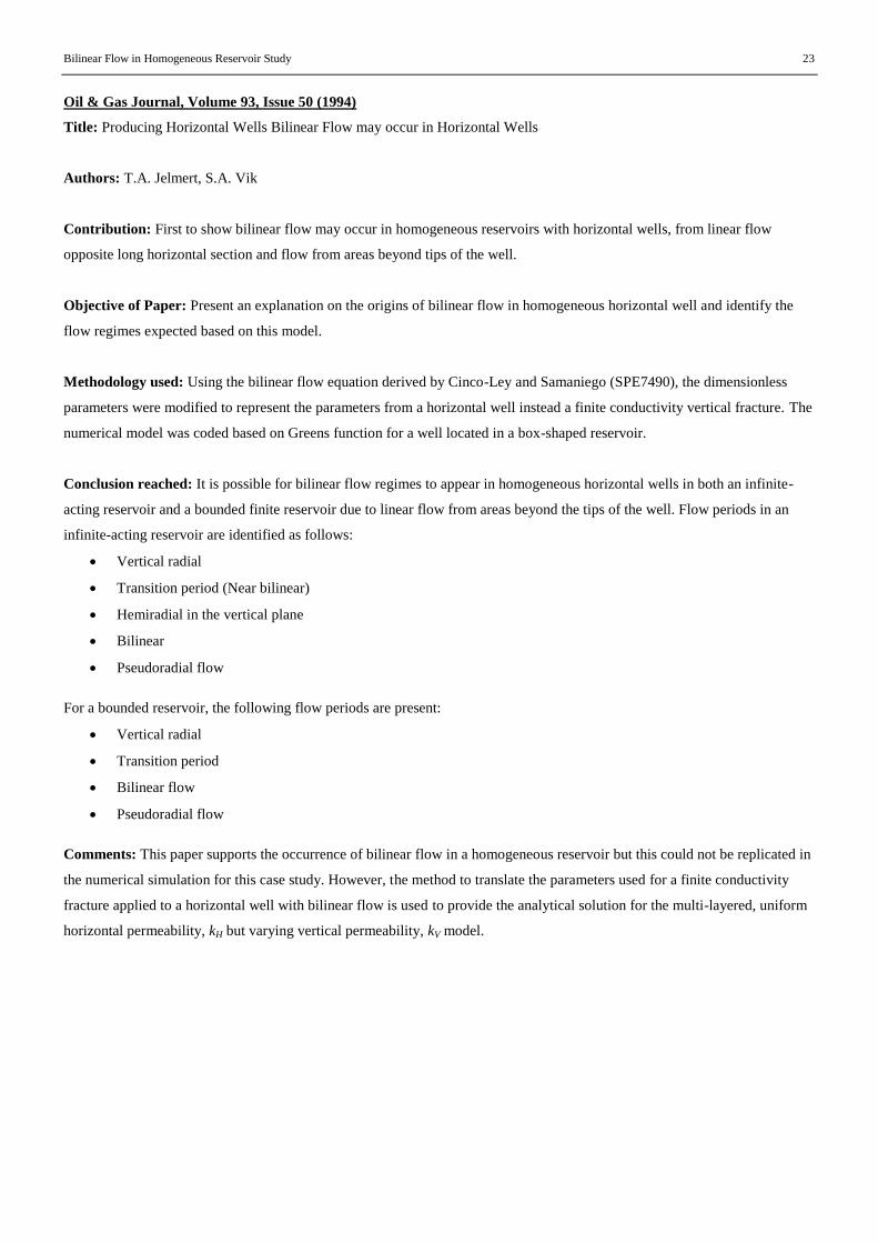
Bilinear Flow in Homogeneous Reservoir Study 23
Oil & Gas Journal, Volume 93, Issue 50 (1994)
Title: Producing Horizontal Wells Bilinear Flow may occur in Horizontal Wells
Authors: T.A. Jelmert, S.A. Vik
Contribution: First to show bilinear flow may occur in homogeneous reservoirs with horizontal wells, from linear flow
opposite long horizontal section and flow from areas beyond tips of the well.
Objective of Paper: Present an explanation on the origins of bilinear flow in homogeneous horizontal well and identify the
flow regimes expected based on this model.
Methodology used: Using the bilinear flow equation derived by Cinco-Ley and Samaniego (SPE7490), the dimensionless
parameters were modified to represent the parameters from a horizontal well instead a finite conductivity vertical fracture. The
numerical model was coded based on Greens function for a well located in a box-shaped reservoir.
Conclusion reached: It is possible for bilinear flow regimes to appear in homogeneous horizontal wells in both an infinite-
acting reservoir and a bounded finite reservoir due to linear flow from areas beyond the tips of the well. Flow periods in an
infinite-acting reservoir are identified as follows:
Vertical radial
Transition period (Near bilinear)
Hemiradial in the vertical plane
Bilinear
Pseudoradial flow
For a bounded reservoir, the following flow periods are present:
Vertical radial
Transition period
Bilinear flow
Pseudoradial flow
Comments: This paper supports the occurrence of bilinear flow in a homogeneous reservoir but this could not be replicated in
the numerical simulation for this case study. However, the method to translate the parameters used for a finite conductivity
fracture applied to a horizontal well with bilinear flow is used to provide the analytical solution for the multi-layered, uniform
horizontal permeability, kH but varying vertical permeability, kV model.

24 Bilinear Flow in Homogeneous Reservoir
SPE 68844 (2001)
Title: Transient Dual-Porosity Behavior for Horizontal Wells Draining Heterogeneous Reservoirs
Authors: F.M. Verga, E. Beretta, D. Albani
Contribution: Exhibited case of bilinear flow when horizontal well intersects a vertical highly-permeable zone surrounded by
a lower permeability zone of an order of magnitude.
Objective of Paper: Present a study of observed bilinear flow when horizontal well intersects with a high-permeability sub-
vertical zone, where linear flow occurs which is “recharged” by linear flow in the surrounding less permeable formation
approaching transient “dual-porosity” behavior.
Methodology used: Using a 3D numerical reservoir model to reproduce the reservoir internal geometry heterogeneity, the
pressure trend monitored at the wells was simulated.
Conclusion reached: Bilinear flow can arise when a horizontal well intersects a highly conductive zone which is fed by
surrounding less permeable formation, provided the permeability contrast is about one order of magnitude.
Comments: This paper indicated that even with permeability contrasts of more than 2 orders of magnitude in the layered
reservoir case introduced by Du and Stewart (1992), they were unable to replicate a ¼ slope straight line in the numerical
simulation. Similar issues were found while modeling this but this was attributed to the thickness of the higher permeability
layer, where beyond a certain thickness the bilinear flow regime is no longer exhibited. However, the authors managed to do
so by modeling the high-permeability sub-vertical zone. In this study, the ¼ slope straight line generated to match the well data
required permeability contrast of 3 orders of magnitude.

Bilinear Flow in Homogeneous Reservoir Study 25
Geological Society of London Publication: The Millennium Atlas: Petroleum Geology of the Central and Northern
North Sea (2003)
Title: “Palaeocene” chapter in “The Millennium Atlas: Petroleum Geology of the Central and Northern North Sea, pg 235-260
Authors: Z.M. Ahmadi, M. Kenyon-Roberts, S. Stanworth, C.W. Kugler, K.A. Kristensen, E.M.G Fugelli; Editors: D. Evans,
C. Graham, C. Armour, P. Bathurst.
Contribution: Characterized the stratigraphy and petroleum geology of the Palaeocene sandstones in submarine fans within
the Central North Sea where the Huntington field is located.
Objective of Paper: Present stratigraphy and petroleum geology of the Palaeocene sands in the North Sea.
Methodology used: Analysis of seismic data, well logs and geological analogues.
Conclusion reached: The Huntington field is considered to be a mid-fan channelized submarine deposit of the Forties
Sandstone Member in the Central Graben, a sand-rich turbidite system that developed during the Palaeocne uplift of the
shoulders of the developing North Atlantic rift. The depositional environment is considered to be dominated by high-density
turbidity currents which led to series of sedimentation waves as currents decelerate and heavier grain populations can no
longer be transported.
Comments: This chapter in the book is heavily referenced by all papers referring to the Palaeocene sandstones in turbidite
submarine fans within the North Sea and is used to understand the geology of the Huntington field.

26 Bilinear Flow in Homogeneous Reservoir
SPE 78969 (2002)
Title: Horizontal Wells Pressure Build Up Analysis in Orinoco Heavy Belt
Authors: M. Briceño, L.E. Summers, O.J. Qujida.
Contribution: Bilinear flow due to compound sands consisting of multiple parasequences (amalgated or separated by shale
barriers).
Objective of Paper: Present integrated analytical approach to pressure build up analysis due to geological complexity of
fluvial-deltaic reservoir sands and peculiar transient pressure behavior.
Methodology used: Using conventional analytical analysis on flow regime identification of well tests with numerical analysis
via a geological numerical simulation model, reservoir characterization of the reservoir was achieved.
Conclusion reached: Bilinear flow is identified in wells completed in sequences or amalgated parasequences of different
permeabilities. This is attributed to the complex depositional environment of the reservoir.
Comments: This paper attributed bilinear flow observed in numerical simulation and well tests to transient double-porosity
model suggested by Du and Stewart (1992). This study showed that this is indeed possible for bilinear flow regime to form
when there is a thin low permeability layer underlying the horizontal well. Although a ¼ slope straight line was reproduced in
this study, this does not match with the well data in this field.

Bilinear Flow in Homogeneous Reservoir Study 27
SPE 159090 (2012)
Title: Estimating Stratigraphic Parameters from Well Test Data in Turbidite Reservoirs
Authors: T. Chen, J. Noirot, A. Khandelwal, G. Xue, M.D. Barton, F.O. Alpak
Contribution: Demonstrated effect of shale drape coverage in reservoir well test analysis of turbidite reservoirs. Channel
shale drape coverage of 0.40 approximate bilinear flow regime.
Objective of Paper: Present well test analysis in turbidite reservoirs and demonstrate effect of fine-scale geological
parameters such as shale drape coverage on pressure transient behavior.
Methodology used: Using reservoir simulation to construct a library of numerical model to match geological features with
well test analysis.
Conclusion reached: Fine-scale stratigraphic parameters such as shale drape coverage and object dimensions (lobe size,
channel width) have a strong impact on well test pressure profiles in turbidite reservoirs.
Comments: This paper suggests that conventional analytical methods for well test analysis are not sufficient for complex
depositional environments in turbidite reservoirs hence the requirement for numerical simulations.

28 Bilinear Flow in Homogeneous Reservoir
SPE 159090 (2012)
Title: Pressure Transient Analyses of Short and Long Duration Well Tests in Unconventional Reservoirs
Authors: B. Kurtoglu, M.A. Torcuk, H.Kazemi
Contribution: Modified the work by (Du & Stewart, 1992), for an analytical solution for transient double-porosity behavior in
a horizontal well.
Objective of Paper: Present an analytical solution for bilinear flow regime due to transient double-porosity behavior in a
horizontal well.
Methodology used: Using numerical inverse Laplace transform as well as closed-form approximate solutions.
Conclusion reached: Analytical solution presented for bilinear flow regime due to transient double-porosity behavior in a
horizontal well. However, it is pointed out by the author that this solution is less reliable because the method requires more
auxiliary data e.g. matrix permeability and shape factor.
Comments: This paper applied a shape factor for spherically-based matrix block in the analytical solution for bilinear flow
due to transient double-porosity behavior in a horizontal well. In this study, the shape factor was modified to a slab model
which represents the reservoir context better.
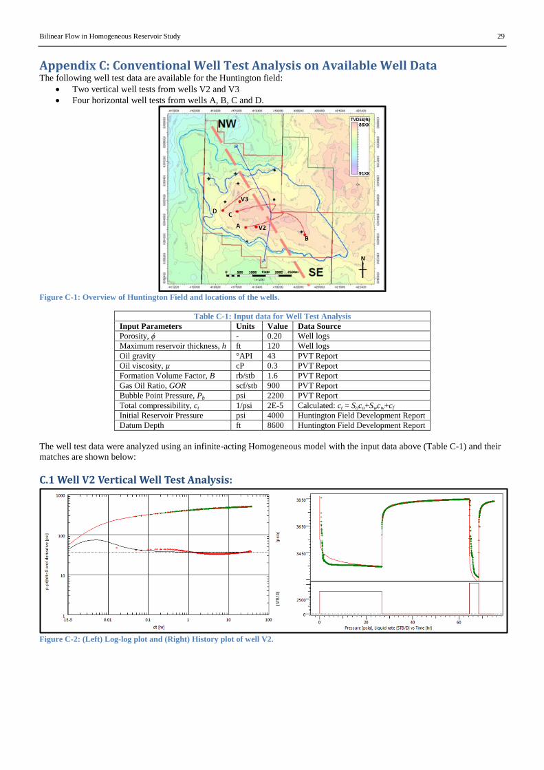
Bilinear Flow in Homogeneous Reservoir Study 29
Appendix C: Conventional Well Test Analysis on Available Well Data The following well test data are available for the Huntington field:
Two vertical well tests from wells V2 and V3
Four horizontal well tests from wells A, B, C and D.
Figure C-1: Overview of Huntington Field and locations of the wells.
Table C-1: Input data for Well Test Analysis Input Parameters Units Value Data Source
Porosity, ϕ - 0.20 Well logs
Maximum reservoir thickness, h ft 120 Well logs
Oil gravity °API 43 PVT Report
Oil viscosity, µ cP 0.3 PVT Report
Formation Volume Factor, B rb/stb 1.6 PVT Report
Gas Oil Ratio, GOR scf/stb 900 PVT Report
Bubble Point Pressure, Pb psi 2200 PVT Report
Total compressibility, ct 1/psi 2E-5 Calculated: ct = Soco+Swcw+cf
Initial Reservoir Pressure psi 4000 Huntington Field Development Report
Datum Depth ft 8600 Huntington Field Development Report
The well test data were analyzed using an infinite-acting Homogeneous model with the input data above (Table C-1) and their
matches are shown below:
C.1 Well V2 Vertical Well Test Analysis:
Figure C-2: (Left) Log-log plot and (Right) History plot of well V2.
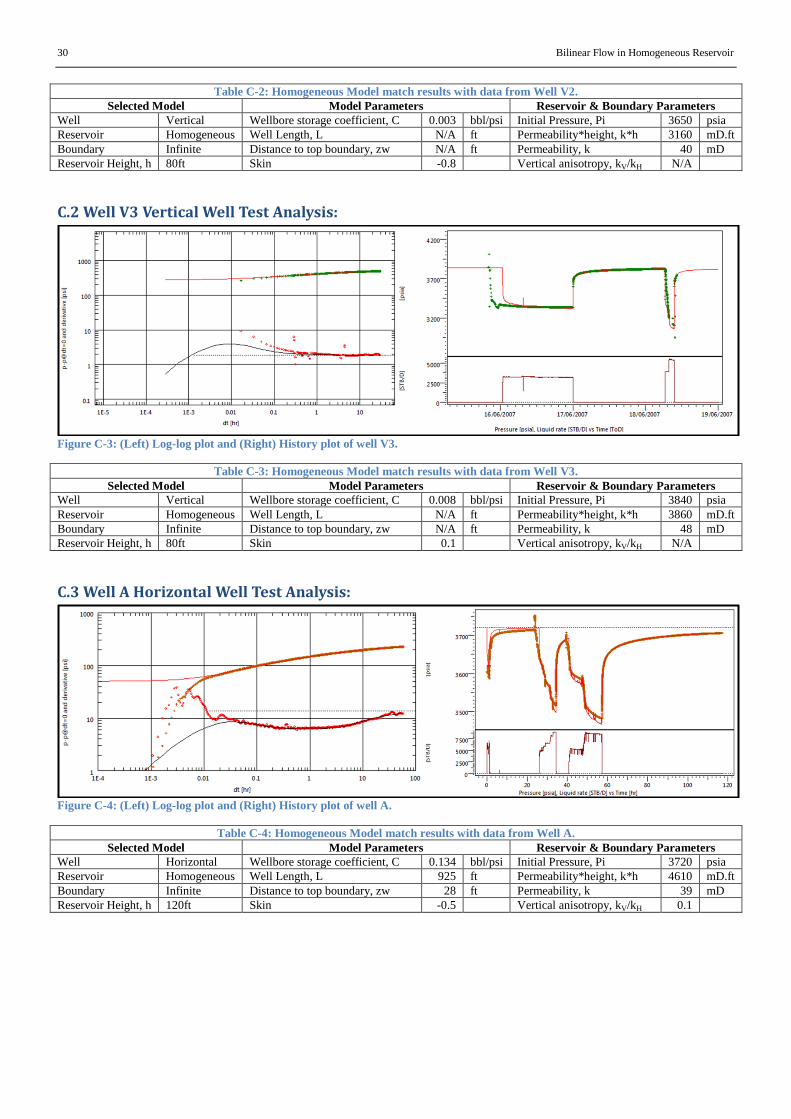
30 Bilinear Flow in Homogeneous Reservoir
Table C-2: Homogeneous Model match results with data from Well V2.
Selected Model Model Parameters Reservoir & Boundary Parameters
Well Vertical Wellbore storage coefficient, C 0.003 bbl/psi Initial Pressure, Pi 3650 psia
Reservoir Homogeneous Well Length, L N/A ft Permeability*height, k*h 3160 mD.ft
Boundary Infinite Distance to top boundary, zw N/A ft Permeability, k 40 mD
Reservoir Height, h 80ft Skin -0.8 Vertical anisotropy, kV/kH N/A
C.2 Well V3 Vertical Well Test Analysis:
Figure C-3: (Left) Log-log plot and (Right) History plot of well V3.
Table C-3: Homogeneous Model match results with data from Well V3.
Selected Model Model Parameters Reservoir & Boundary Parameters
Well Vertical Wellbore storage coefficient, C 0.008 bbl/psi Initial Pressure, Pi 3840 psia
Reservoir Homogeneous Well Length, L N/A ft Permeability*height, k*h 3860 mD.ft
Boundary Infinite Distance to top boundary, zw N/A ft Permeability, k 48 mD
Reservoir Height, h 80ft Skin 0.1 Vertical anisotropy, kV/kH N/A
C.3 Well A Horizontal Well Test Analysis:
Figure C-4: (Left) Log-log plot and (Right) History plot of well A.
Table C-4: Homogeneous Model match results with data from Well A.
Selected Model Model Parameters Reservoir & Boundary Parameters
Well Horizontal Wellbore storage coefficient, C 0.134 bbl/psi Initial Pressure, Pi 3720 psia
Reservoir Homogeneous Well Length, L 925 ft Permeability*height, k*h 4610 mD.ft
Boundary Infinite Distance to top boundary, zw 28 ft Permeability, k 39 mD
Reservoir Height, h 120ft Skin -0.5 Vertical anisotropy, kV/kH 0.1

Bilinear Flow in Homogeneous Reservoir Study 31
C.4 Well B Horizontal Well Test Analysis:
Figure C-5: (Left) Log-log plot and (Right) History plot of well B.
Table C-5: Homogeneous Model match results with data from Well B.
Selected Model Model Parameters Reservoir & Boundary Parameters
Well Horizontal Wellbore storage coefficient, C 0.406 bbl/psi Initial Pressure, Pi 3680 psia
Reservoir Homogeneous Well Length, L 974 ft Permeability*height, k*h 4190 mD.ft
Boundary Infinite Distance to top boundary, zw 59 ft Permeability, k 52 mD
Reservoir Height, h 80ft Skin -0.4 Vertical anisotropy, kV/kH 0.4
C.5 Well C Horizontal Well Test Analysis:
Figure C-6: (Left) Log-log plot and (Right) History plot of well C.
Table C-6: Homogeneous Model match results with data from Well C.
Selected Model Model Parameters Reservoir & Boundary Parameters
Well Horizontal Wellbore storage coefficient, C 0.011 bbl/psi Initial Pressure, Pi 3640 psia
Reservoir Homogeneous Well Length, L 349 ft Permeability*height, k*h 7520 mD.ft
Boundary Infinite Distance to top boundary, zw 59 ft Permeability, k 63 mD
Reservoir Height, h 120ft Skin -0.9 Vertical anisotropy, kV/kH 0.7

32 Bilinear Flow in Homogeneous Reservoir
C.6 Well D Horizontal Well Test Analysis:
Figure C-7: (Left) Log-log plot and (Right) History plot of well D.
Table C-7: Homogeneous Model match results with data from Well D.
Selected Model Model Parameters Reservoir & Boundary Parameters
Well Horizontal Wellbore storage coefficient, C 0.016 bbl/psi Initial Pressure, Pi 3654 psia
Reservoir Homogeneous Well Length, L 640 ft Permeability*height, k*h 4590 mD.ft
Boundary Infinite Distance to top boundary, zw 18 ft Permeability, k 39 mD
Reservoir Height, h 120ft Skin -0.5 Vertical anisotropy, kV/kH 0.3
C.7 Summary: In summary, except for Well A, the other horizontal wells do not match a homogeneous model very well:
Table C-8: Summary of well test results.
Well Name: Model Used: k*h (mD.ft) kH (mD) L (ft) h (ft)
V2 Homogeneous 3,160 40 - 80
V3 Homogeneous 3,860 48 - 80
A Homogeneous 4,610 39 925 120
B Homogeneous 4,190 52 974 80
C Homogeneous 7,520 63 349 120
D Homogeneous 4,590 39 690 120

Bilinear Flow in Homogeneous Reservoir Study 33
Appendix D: Modified Pulse Tests The following are the history plots of the modified pulse tests performed in the Huntington Field, showing the time lag and
pressure drop:
Figure D-1: History plot of modified pulse test between Well A (Active) and Well C (Observation).
Figure D-2: History plot of modified pulse test between Well D (Active) and Well C (Observation).
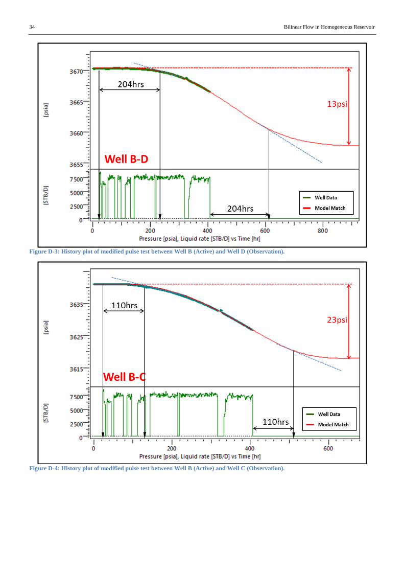
34 Bilinear Flow in Homogeneous Reservoir
Figure D-3: History plot of modified pulse test between Well B (Active) and Well D (Observation).
Figure D-4: History plot of modified pulse test between Well B (Active) and Well C (Observation).
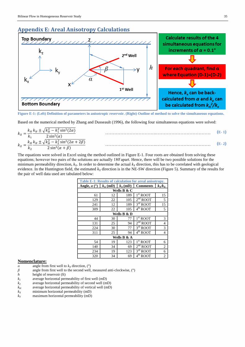
Bilinear Flow in Homogeneous Reservoir Study 35
Appendix E: Areal Anisotropy Calculations
Figure E-1: (Left) Definition of parameters in anisotropic reservoir. (Right) Outline of method to solve the simultaneous equations.
Based on the numerical method by Zhang and Dusseault (1996), the following four simultaneous equations were solved:
√
( )
( ) …………………………….……………………………… (E- 1)
√
( )
( ) …………………………….……………………………… (E- 2)
The equations were solved in Excel using the method outlined in Figure E-1. Four roots are obtained from solving these
equations however two pairs of the solutions are actually apart. Hence, there will be two possible solutions for the
minimum permeability direction, kX. In order to determine the actual kX direction, this has to be correlated with geological
evidence. In the Huntington field, the estimated kX direction is in the NE-SW direction (Figure 5). Summary of the results for
the pair of well data used are tabulated below:
Table E-1: Results of calculation for areal anisotropy.
Angle, α (°) kX (mD) kY (mD) Comments kY/kX
Wells B & C
61 12 189 1st ROOT 15
129 22 105 2nd ROOT 5
241 12 189 3rd ROOT 15
309 22 105 4th ROOT 5
Wells B & D
44 30 77 1st ROOT 3
131 25 94 2nd ROOT 4
224 30 77 3rd ROOT 3
311 25 94 4th ROOT 4
Wells B & A
54 19 123 1st ROOT 6
140 34 69 2nd ROOT 2
234 19 123 3rd ROOT 6
320 34 69 4th ROOT 2
Nomenclature: α angle from first well to kX direction, (°)
β angle from first well to the second well, measured anti-clockwise, (°)
h height of reservoir (ft)
k1 average horizontal permeability of first well (mD)
k2 average horizontal permeability of second well (mD)
kH average horizontal permeability of vertical well (mD)
kX minimum horizontal permeability (mD)
kY maximum horizontal permeability (mD)

36 Bilinear Flow in Homogeneous Reservoir
Appendix F: Base Model Behavior The analytical solutions from Ozkan and Raghavan (1991) were used to compare the base model results in order to validate the
model behavior. It is important that the model is validated so that no additional parameters will be introduced which may
affect the conclusion of this study. The following parameters were varied:
L, total length of horizontal well
kV/kH, vertical permeability anisotropy ratio in reservoir
zw, distance to top boundary of reservoir
kY/kX, areal permeability anisotropy ratio in reservoir
based on the following definitions keeping kH = 100mD, h = 100ft:
Figure F-1: Definition of well parameters in simulation.
The comparison shows that the simulation results matches well with the analytical solutions:
Figure F-2: Comparison of base model behavior with analytical solution by Ozkan & Raghavan, 1991 (Black-dots)

Bilinear Flow in Homogeneous Reservoir Study 37
Appendix G: Sensitivity Analysis of Numerical Simulation Results Specific cases where the simulation data closely matches the well data were detailed earlier in Section 4.3. This section shows
the sensitivity of the geological features being modeled as well parameters are varied.
G.1 Horizontal well intersecting a High-Permeability Streak The permeability contrast between the high-permeability streak and its surroundings is varied from 1 to 3 orders of magnitude
while maintaining the average horizontal permeability, kH = 40mD. It can be observed that the slope of the derivative flattens
in early-time as the permeability contrast is reduced (Figure G-1).
Figure G-1: Sensitivity to change in the order of permeability contrast magnitude in high-permeability streak model.
Figure G-2: Sensitivity to change in the width of the high-permeability streak model.
The sensitivity to the change in width of the high-permeability streak model was also modeled maintaining kH = 40mD and
permeability contrast of 3 orders of magnitude. It can be observed that the slope becomes steeper approaching linear flow (½
slope) as the width of the high-permeability streak is increased (Figure G-2).

38 Bilinear Flow in Homogeneous Reservoir
Figure G-3: Sensitivity to change in kV/kH of the 100ft-wide 10-10,000mD high-permeability streak model.
Finally, the sensitivity to the change in vertical permeability anisotropy ratio, kV/kH is modeled for the 100-ft wide 10,000mD
high-permeability streak surrounded by 10mD matrix. It is shown that a change in kV/kH predominantly changes the early-time
derivative behavior (Figure G-3).
G.2 Dual layer formation with Higher-Permeability layer overlying Lower-Permeability layer Du and Stewart (1992) mentioned in their paper that a permeability contrast of at least one order of magnitude is required for
the bilinear flow regime to form in a 2-layer formation with higher permeability layer overlying the lower permeability layer.
The permeability contrast of this model is varied from ½ order of magnitude to 2 orders of magnitude. It is found that the slope
of the derivative flattens as the permeability contrast is reduced (½ order of magnitude) and it steepens slightly when the
permeability contrast is increased (2 orders of magnitude) (Figure G-4).
Figure G-4: Sensitivity to change in permeability contrast between the 2 layers.

Bilinear Flow in Homogeneous Reservoir Study 39
Figure G-5: Sensitivity to change in thickness of the 2 layers.
When the thickness of the 2 layers are varied with L1 representing the top layer and L2 the bottom layer while maintaining a
total reservoir height, h of 120ft and an average horizontal permeability, kH of 50mD; it is found that a thinner L1 flattens the
derivative while a thicker L1 steepens the derivative, approaching ½ slope (Figure G-5). Note that if L1 thickness is higher,
then the ¼ slope straight line will not appear at all. This explains why Verga et al. (2001) was not able to reproduce the
transient double-porosity behavior in his simulations.
Maintaining the 2 layers to the same permeability contrast of 250-25mD and thickness of 15-105ft, the effect of the vertical
permeability anisotropy ratio, kV/kH is modeled. It is observed that as kV/kH is increased, it leads to a flattening of the derivative
and causes the linear flow regime to start earlier (Figure G-6).
Figure G-6: Sensitivity to change in kV/kH of the model.
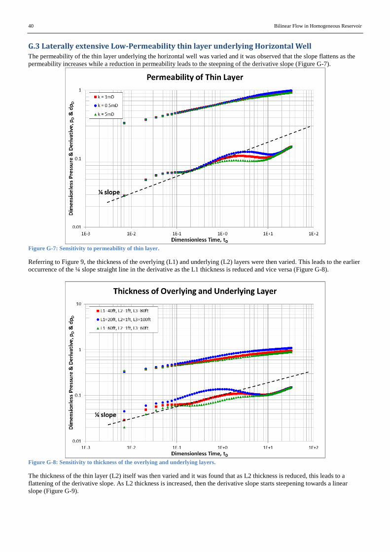
40 Bilinear Flow in Homogeneous Reservoir
G.3 Laterally extensive Low-Permeability thin layer underlying Horizontal Well The permeability of the thin layer underlying the horizontal well was varied and it was observed that the slope flattens as the
permeability increases while a reduction in permeability leads to the steepning of the derivative slope (Figure G-7).
Figure G-7: Sensitivity to permeability of thin layer.
Referring to Figure 9, the thickness of the overlying (L1) and underlying (L2) layers were then varied. This leads to the earlier
occurrence of the ¼ slope straight line in the derivative as the L1 thickness is reduced and vice versa (Figure G-8).
Figure G-8: Sensitivity to thickness of the overlying and underlying layers.
The thickness of the thin layer (L2) itself was then varied and it was found that as L2 thickness is reduced, this leads to a
flattening of the derivative slope. As L2 thickness is increased, then the derivative slope starts steepening towards a linear
slope (Figure G-9).
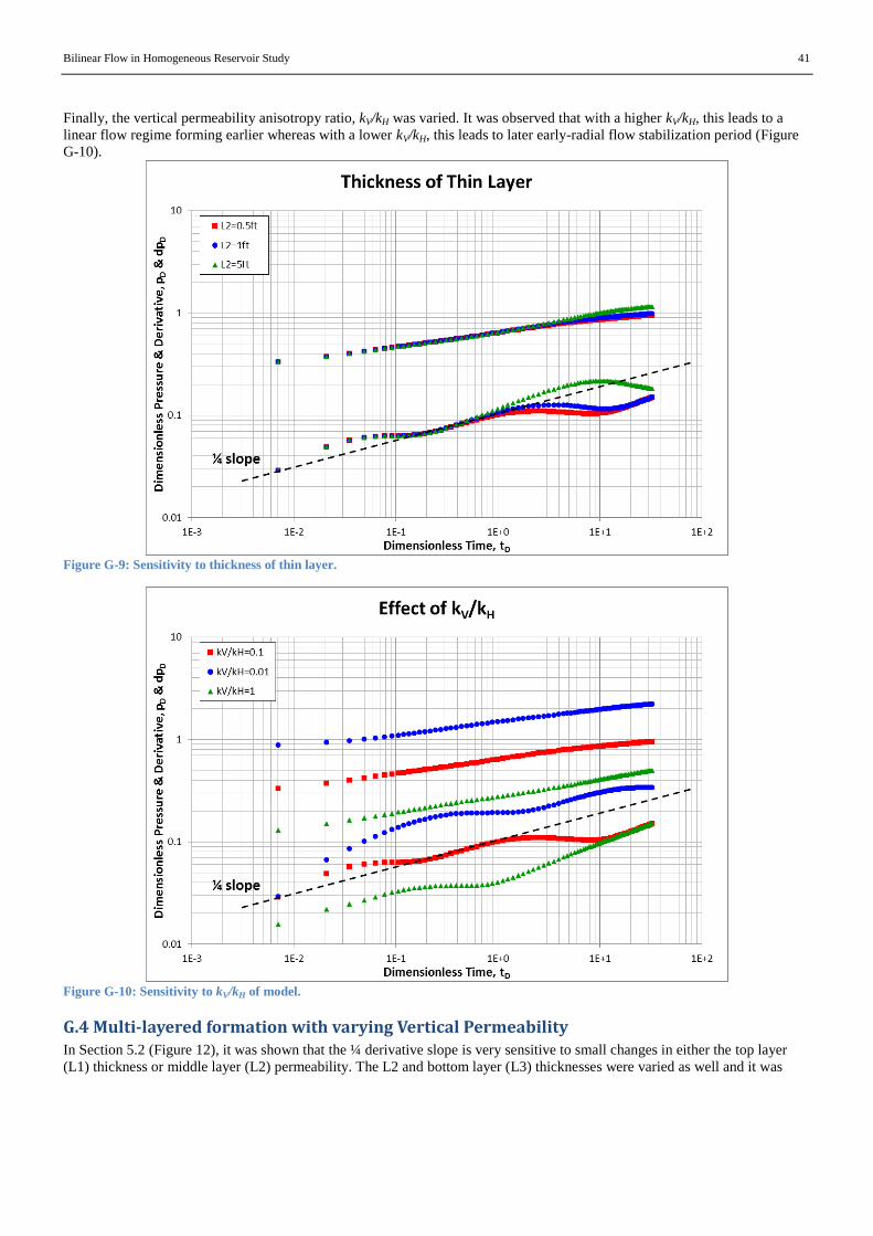
Bilinear Flow in Homogeneous Reservoir Study 41
Finally, the vertical permeability anisotropy ratio, kV/kH was varied. It was observed that with a higher kV/kH, this leads to a
linear flow regime forming earlier whereas with a lower kV/kH, this leads to later early-radial flow stabilization period (Figure
G-10).
Figure G-9: Sensitivity to thickness of thin layer.
Figure G-10: Sensitivity to kV/kH of model.
G.4 Multi-layered formation with varying Vertical Permeability In Section 5.2 (Figure 12), it was shown that the ¼ derivative slope is very sensitive to small changes in either the top layer
(L1) thickness or middle layer (L2) permeability. The L2 and bottom layer (L3) thicknesses were varied as well and it was

42 Bilinear Flow in Homogeneous Reservoir
observed that when L2 thickness is decreased, this leads to a steepening of the slope in early-time whereas an increase in L2
thickness causes a flattening of the derivative slope (Figure G-11).
However, it appears that the ¼ slope straight line is relatively insensitive to L3 thickness (Figure G-12). Even when there are
4-layers in the model, the ¼ slope straight line is also insensitive to the vertical permeability in the fourth layer (Figure 14).
Figure G-11: Sensitivity to L2 thickness of the model.
Figure G-12: Sensitivity to L3 thickness of the model.
When varying the vertical permeability, kV of the individual layers, it was also observed that the ¼ slope straight line is
relatively insensitive to the kV in L1 (Figure G-13). However, increasing kV in L3 leads to a flattening of the ¼ slope straight
line in late-intermediate time while reducing the kV in L3 causes the reverse (Figure G-14).

Bilinear Flow in Homogeneous Reservoir Study 43
Figure G-13: Sensitivity to L1 vertical permeability.
Figure G-14: Sensitivity to L3 vertical permeability.
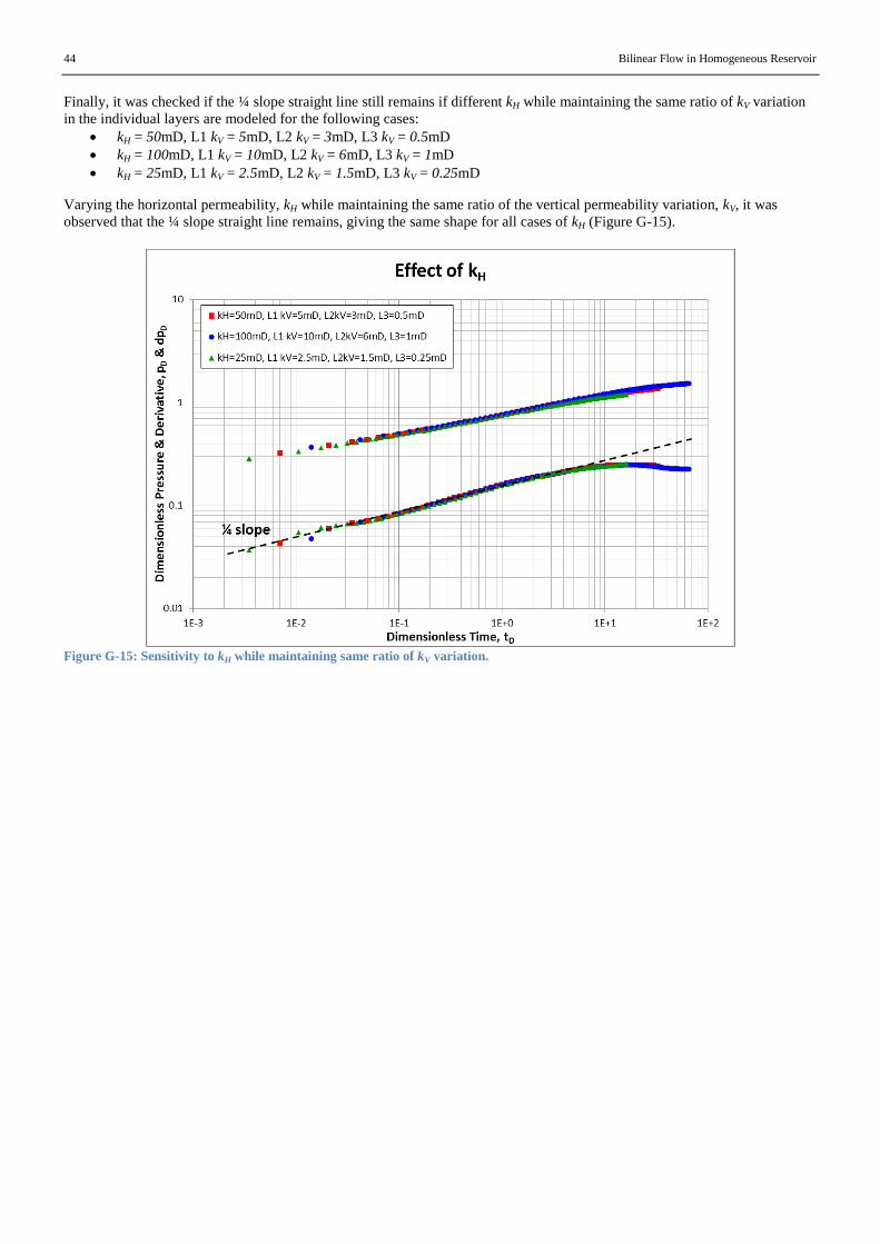
44 Bilinear Flow in Homogeneous Reservoir
Finally, it was checked if the ¼ slope straight line still remains if different kH while maintaining the same ratio of kV variation
in the individual layers are modeled for the following cases:
kH = 50mD, L1 kV = 5mD, L2 kV = 3mD, L3 kV = 0.5mD
kH = 100mD, L1 kV = 10mD, L2 kV = 6mD, L3 kV = 1mD
kH = 25mD, L1 kV = 2.5mD, L2 kV = 1.5mD, L3 kV = 0.25mD
Varying the horizontal permeability, kH while maintaining the same ratio of the vertical permeability variation, kV, it was
observed that the ¼ slope straight line remains, giving the same shape for all cases of kH (Figure G-15).
Figure G-15: Sensitivity to kH while maintaining same ratio of kV variation.

Bilinear Flow in Homogeneous Reservoir Study 45
Appendix H: Analytical Solutions to Bilinear Flow Regime Straight-line analysis of the slope of √
was used to calculate the input parameters of the simulation results from the 3-
layer, uniform kH and varying kV model of Well C. It is found that two models can be used:
Finite Conductivity Fracture Model
Transient Double-Porosity Model
H.1 Finite Conductivity Fracture Model:
The solution by Cinco-Ley and Samaniego-V (1981) for a straight-line analysis on plot of √
is:
( ) ( )
………………………..…………………………….…………………… (H- 1)
Jelmert and Vik (1995) modified the equation above so that the well parameters defining a finite conductivity fracture is
translated into the case for a bilinear flow where the primary linear flow in the layer containing the horizontal well supported
by a secondary linear flow in the supporting layer (Figure H-1).
Figure H-1: Translation of parameters from finite-conductivity fracture model to horizontal well with varying kV model.
This resulted in an equation as follows:
( ) ( )
………………………..…………………………….…………………… (H- 2)
Equation (H- 2) was used to analyze the straight-line slope with the following results:
Table H-1: Calculation of kVE using modified Finite Conductivity Fracture model
Straight-line slope, mblf 88.36
Length of well, h (ft) 3000
Height of Layer 1, hL1 (ft) 15
Oil flowrate, q (stb/d) 10500
Oil viscosity, µ (cP) 0.29
Oil formation volume factor, B(rb/stb) 1.585
Porosity, ϕ 0.2
Total compressibility, ct (1/psi) 2×10⁵
Horizontal permeability, kH (mD) 50
Equivalent vertical permeability, kVE (mD) 0.64

46 Bilinear Flow in Homogeneous Reservoir
Equation used for harmonic-averaging of the vertical permeability, for the 3-layer model, n = 3:
∑
∑
………………………..…………………………….…………………………………………….
(H- 3)
The calculated kVE of 0.64mD is very close to the harmonic averaged permeability, kV’ of the 3-layer, uniform kH and varying
kV model of 0.61mD:
Figure H-2: Graphical representation of dimensions and well parameters used in the 3-layer, uniform kH, varying kV model.
H.2 Transient Double Porosity Model: Du and Stewart (1992) introduced the concept of bilinear flow due to transient double porosity behavior in a horizontal well.
However, their derived equation results in the cancellation of the fracture permeability term:
√ {
( )
}
……………………………….…………………… (H- 4)
Kurtoglu et al. (2012) re-derived the solution and came up with the following equation but applied it using a spherical-matrix
block model to a fractured reservoir:
√ {
( ) [
( ) ]
}
……………………………….…………………… (H- 5)
In this study, as the transient double-porosity is applied to a reservoir with uniform horizontal permeability, kH; uniform
porosity, ϕ and total compressibility, ct. The storativity ratio is hence simply the ratio of the height of the more permeable layer
to the total height of the reservoir:
………………………………………………………………………………….…………………… (H- 6)
Following the rationale by Du and Stewart (1992) that a slab model better represents the bilinear flow regime in a layered
reservoir, the shape factor of a slab model was used:
………………………………………………………………………………….……………………
(H- 7)
The above equation can then be expressed as follows:
√
{
(
)
[
]
}
……………………………….…………………… (H- 8)
Assuming the fracture permeability, kf as the highest permeability i.e. the uniform horizontal permeability, kH and the averaged
vertical permeability, kV’ as the matrix permeability, km; it is found that the calculated matrix permeability is close to the
harmonic average of the top 2 layers of the model (3.95mD).
Equation (H- 8) was used to analyze the straight-line slope with the following results:

Bilinear Flow in Homogeneous Reservoir Study 47
Table H-2: Calculation of km using modified Transient Double Porosity model
Straight-line slope, mblf 88
Wellbore radius, rw (ft) 0.46
Oil flowrate, q (stb/d) 10500
Oil viscosity, µ (cP) 0.3
Oil formation volume factor, B(rb/stb) 1.6
Porosity, ϕ 0.20
Total compressibility, ct (1/psi) 2×10⁵
Height of L1, hL1 (ft) 15
Total height of reservoir, htotal (ft) 120
Length of well, L (ft) 3000
Fracture permeability, kf (mD) 50
Matrix permeability, km (mD) 4.25
Nomenclature: β β = n + 2, constant expressing the results of semi-steady-state flow in linear (n=1), radial cylindrical (n=2) and spherical (n=3).
µ viscosity (cP)
ω storativity ratio
ϕ porosity
σ shape factor
B oil formation volume factor (rb/stb)
bf width of fracture (ft)
ct total compressibility (1/psi)
h height of reservoir (ft)
hL1 height of more permeable layer (ft)
hi height of individual layer in model (ft)
htotal total height of reservoir (ft)
kf fracture permeability (mD)
kH horizontal permeability (mD)
km matrix permeability (mD)
kV’ harmonic averaged vertical permeability (mD)
kVE equivalent vertical permeability (mD)
kVi vertical permeability of individual layer in model (mD)
L length of horizontal well (ft)
q oil production rate (stb/d)
sma interporosity skin
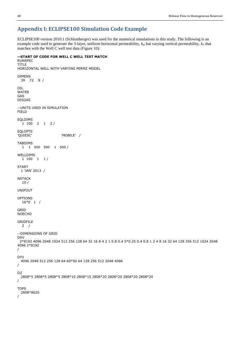
48 Bilinear Flow in Homogeneous Reservoir
Appendix I: ECLIPSE100 Simulation Code Example
ECLIPSE100 version 2010.1 (Schlumberger) was used for the numerical simulations in this study. The following is an
example code used to generate the 3-layer, uniform horizontal permeability, kH but varying vertical permeability, kV that
matches with the Well C well test data (Figure 10): --START OF CODE FOR WELL C WELL TEST MATCH RUNSPEC TITLE HORIZONTAL WELL WITH VARYING PERMZ MODEL DIMENS 39 72 9 / OIL WATER GAS DISGAS --UNITS USED IN SIMULATION FIELD EQLDIMS 1 100 2 1 2 / EQLOPTS 'QUIESC' 'MOBILE' / TABDIMS
1 1 500 500 1 500 / WELLDIMS 1 100 1 1 / START 1 'JAN' 2013 / NSTACK 10 / UNIFOUT OPTIONS 16*0 1 / GRID NOECHO GRIDFILE 2 / --DIMENSIONS OF GRID DXV 2*8192 4096 2048 1024 512 256 128 64 32 16 8 4 2 1 0.8 0.4 5*0.25 0.4 0.8 1 2 4 8 16 32 64 128 256 512 1024 2048 4096 2*8192 / DYV 4096 2048 512 256 128 64 60*50 64 128 256 512 2048 4096 / DZ 2808*5 2808*5 2808*5 2808*10 2808*15 2808*20 2808*20 2808*20 2808*20 / TOPS 2808*8620 /

Bilinear Flow in Homogeneous Reservoir Study 49
--POROSITY AND PERMEABILITY OF GRID CELLS EQUALS 'PORO' 0.2 / / PERMX 25272*50 / PERMY 25272*50 / PERMZ 2808*5 2808*5 2808*5 2808*3 2808*0.5 2808*0.5 2808*0.5 2808*0.5 2808*0.5 / INIT RPTGRID 'ALLNNC' / EDIT PROPS
INCLUDE 'MSC_PROPS.INC' / REGIONS SOLUTION RSVD 8200.0 0.878192 8900.0 0.878192 / EQUIL 8640 3890.00 8800.00 0.00000 6100.00 0.00000 1 0 10 / DATUM 8640 / RPTSOL 'SWAT' 'SGAS' 'RESTART=2' 'FIP=1' / SUMMARY FOPR FWCT FGOR FOPT TIMESTEP WBHP / WOPR / --SIMULATION SCHEDULED TO RUN A DRAWDOWN OF 24HRS FOLLOWED BY BUILDUP OF 24HRS SCHEDULE INCLUDE 'MSC_SCH.INC' / --END OF CODE *The PROPS & SCH file is included in the CD.