a triple-porosity model for fractured horizontal wells

A TRIPLE-POROSITY MODEL FOR FRACTURED HORIZONTAL WELLS

A Thesis

by

HASAN ALI H ALAHMADI

Submitted to the Office of Graduate Studies of

Texas A&M University

in partial fulfillment of the requirements for the degree of

MASTER OF SCIENCE

August 2010

Major Subject: Petroleum Engineering

A Triple-Porosity Model for Fractured Horizontal Wells

Copyright 2010 Hasan Ali H Alahmadi

A TRIPLE-POROSITY MODEL FOR FRACTURED HORIZONTAL WELLS

A Thesis

by

HASAN ALI H ALAHMADI

Submitted to the Office of Graduate Studies of

Texas A&M University

in partial fulfillment of the requirements for the degree of

MASTER OF SCIENCE

Approved by:

Chair of Committee, Robert A. Wattenbarger

Committee Members, J. Bryan Maggard

William Rundell

Head of Department, Stephen A. Holditch

August 2010

Major Subject: Petroleum Engineering

iii

ABSTRACT

A Triple-Porosity Model for Fractured Horizontal Wells. (August 2010)

Hasan Ali H Alahmadi, B.Sc., King Fahd University of Petroleum and Minerals

Chair of Advisory Committee: Dr. Robert A. Wattenbarger

Fractured reservoirs have been traditionally idealized using dual-porosity models.

In these models, all matrix and fractures systems have identical properties. However, it

is not uncommon for naturally fractured reservoirs to have orthogonal fractures with

different properties. In addition, for hydraulically fractured reservoirs that have pre-

existing natural fractures such as shale gas reservoirs, it is almost certain that these types

of fractures are present. Therefore, a triple-porosity (dual-fracture) model is developed in

this work for characterizing fractured reservoirs with different fractures properties.

The model consists of three contiguous porous media: the matrix, less permeable

micro-fractures and more permeable macro-fractures. Only the macro-fractures produce

to the well while they are fed by the micro-fractures only. Consequently, the matrix

feeds the micro-fractures only. Therefore, the flow is sequential from one medium to the

other.

Four sub-models are derived based on the interporosity flow assumption between

adjacent media, i.e., pseudosteady state or transient flow assumption. These are fully

transient flow model (Model 1), fully pseudosteady state flow model (Model 4) and two

mixed flow models (Model 2 and 3).

iv

The solutions were mainly derived for linear flow which makes this model the

first triple-porosity model for linear reservoirs. In addition, the Laplace domain solutions

are also new and have not been presented in the literature before in this form.

Model 1 is used to analyze fractured shale gas horizontal wells. Non-linear

regression using least absolute value method is used to match field data, mainly gas rate.

Once a match is achieved, the well model is completely described. Consequently,

original gas in place (OGIP) can be estimated and well future performance can be

forecasted.

v

DEDICATION

To my parents for their love, sacrifices and prayers.

To my beloved wife, Asmaa, for her love, patience and support throughout my study.

To my adorable son, Hatem, (our little Aggie who was born while I was working on this

research and turned one when I defended it), for the joy and happiness he has brought to

my life.

vi

ACKNOWLEDGEMENTS

All praises and thanks to Allah almighty, the Lord of the entire creation that

exists, for His infinite mercies and abundant blessings.

I would like to thank my committee chair, Dr. Robert Wattenbarger, for his

support, guidance and inspiration throughout this research. I was honored to work with

him.

I would also like to thank Dr. Maggard and Dr. Rundell for serving on my

advisory committee and for their constructive feedback which helps making this work

better.

In addition, I would like to express my gratitude to Saudi Aramco for giving me

the chance to pursue my advanced degree and sponsoring my study at Texas A&M

University.

Thanks to my colleagues at the Reservoir Modeling Consortium for their

informative discussions and friendship; namely, Hassan Hamam, Salman Mengal, Tan

Tran, Pahala Sinurat, Anas Almarzooq, Haider Abdulaal, Orkhan Samandarli and

Ammar Agnia.

Thanks also go to my friends, colleagues and the Petroleum Engineering

department faculty and staff for making my time at Texas A&M University a great

experience.

Finally, thanks to Saudi Students Association for their support and making

College Station our second home.

vii

TABLE OF CONTENTS

Page

ABSTRACT .............................................................................................................. iii

DEDICATION .......................................................................................................... v

ACKNOWLEDGEMENTS ...................................................................................... vi

TABLE OF CONTENTS .......................................................................................... vii

LIST OF FIGURES ................................................................................................... x

LIST OF TABLES .................................................................................................... xiii

CHAPTER

I INTRODUCTION ................................................................................ 1

1.1 Motivation ................................................................................... 2

1.2 Objectives .................................................................................... 2

1.3 Organization of the Thesis .......................................................... 3

II LITERATURE REVIEW ..................................................................... 4

2.1 Dual-porosity Models ................................................................... 4

2.1.1 Pseudosteady State Models ................................................ 4

2.1.2 Unsteady State Models ...................................................... 5

2.2 Triple-porosity Models ................................................................. 6

2.3 Linear Flow in Fractured Reservoirs ............................................ 9

III TRIPLE-POROSITY MODEL FOR FRACTURED RESERVOIRS:

NEW SOLUTIONS .............................................................................. 11

3.1 Introduction .................................................................................. 11

3.2 Linear Flow Solutions for Linear Fractured Reservoirs .............. 12

3.3 Derivations of the Triple-porosity Analytical Solutions .............. 12

3.3.1 Model Assumptions .......................................................... 13

3.3.2 Definitions of Dimensionless Variables ............................ 14

3.3.3 Model 1: Fully Transient Triple-porosity Model ............... 15

3.3.4 Model 2: Mixed Flow Triple-porosity Model.................... 18

viii

CHAPTER Page

3.3.5 Model 3: Mixed Flow Triple-porosity Model.................... 19

3.3.6 Model 4: Fully PSS Triple-porosity Model ....................... 19

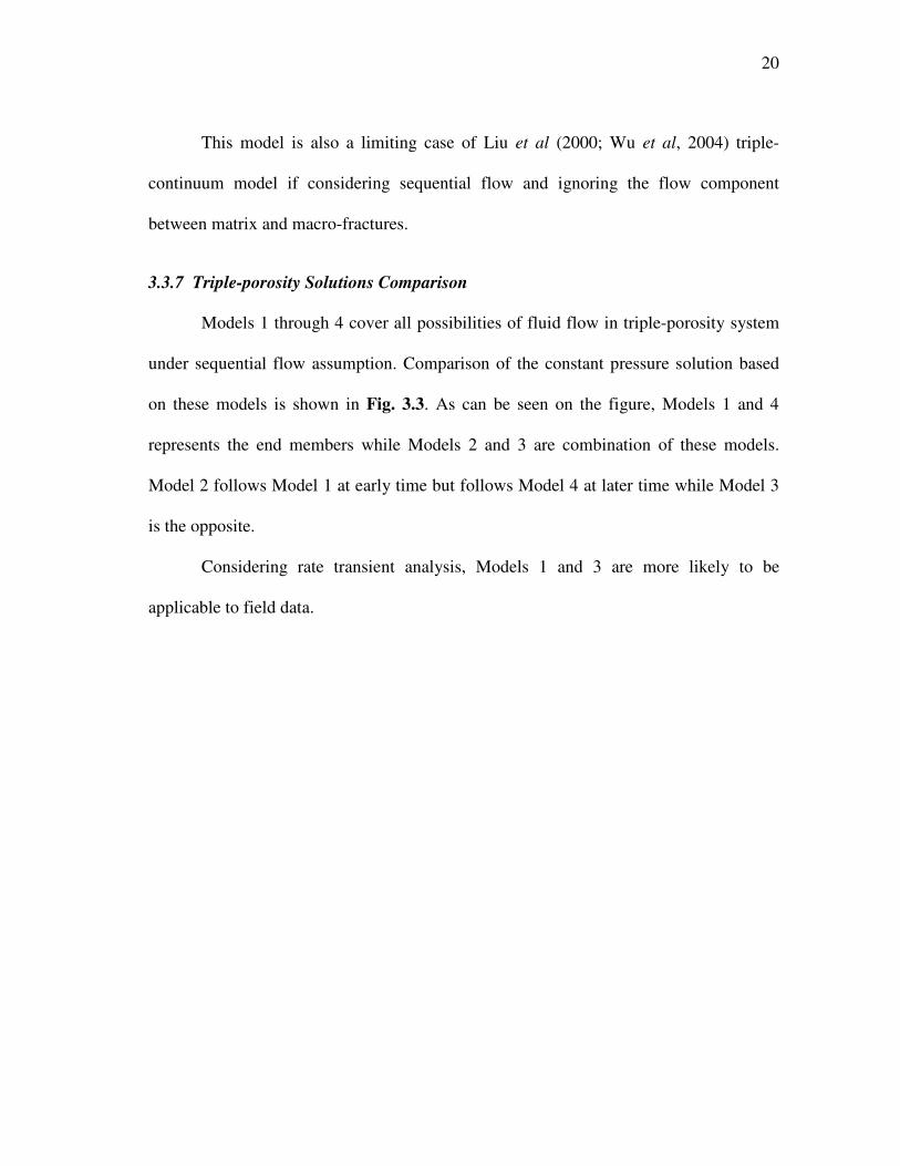
3.3.7 Triple-porosity Solutions Comparison............................... 20

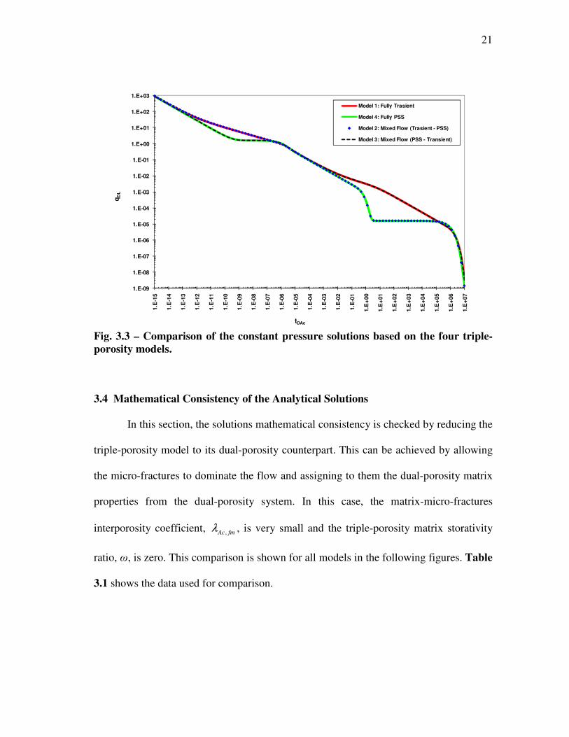
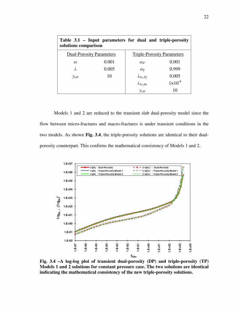
3.4 Mathematical Consistency of the Analytical Solutions ............... 21

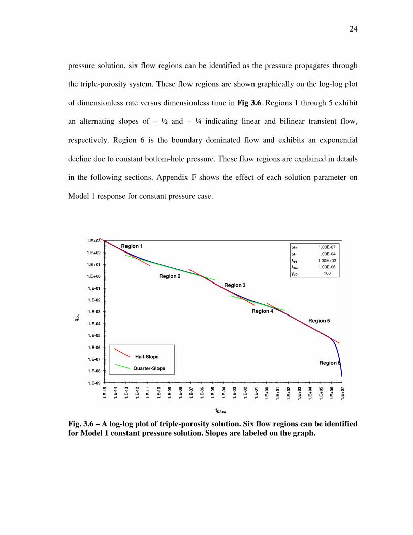
3.5 Flow Regions Based on the Analytical Solution .......................... 23

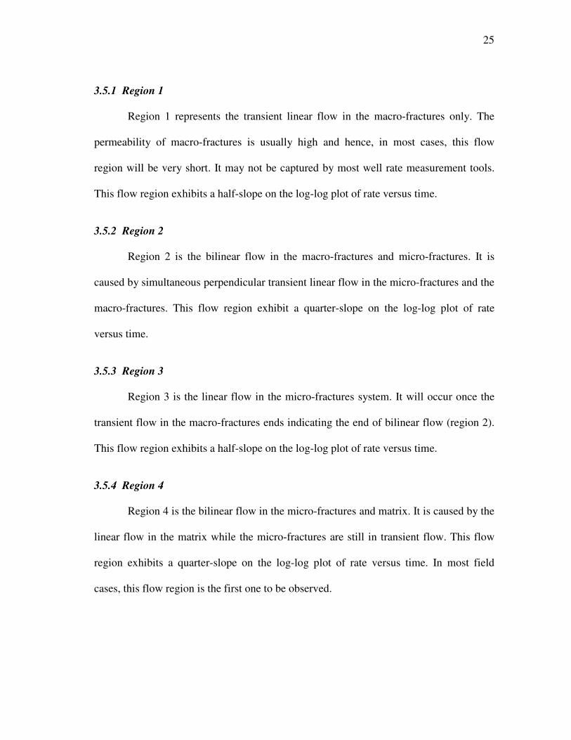
3.5.1 Region 1 ............................................................................. 25

3.5.2 Region 2 ............................................................................. 25

3.5.3 Region 3 ............................................................................. 25

3.5.4 Region 4 ............................................................................. 25

3.5.5 Region 5 ............................................................................. 26

3.5.6 Region 6 ............................................................................. 26

3.6 Triple-porosity Solutions for Radial Flow ................................... 26

3.7 Application to Gas Flow .............................................................. 28

3.8 Chapter Summary ......................................................................... 29

IV TRIPLE-POROSITY SIMULATION MODEL AND

ANALYTICAL SOLUTIONS VERIFICATION ................................ 30

4.1 Introduction .................................................................................. 30

4.2 Simulation Model Description ..................................................... 30

4.3 Analytical Solution Validation ..................................................... 31

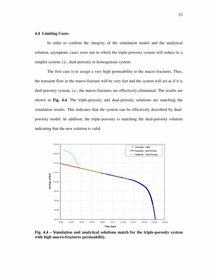
4.4 Limiting Cases .............................................................................. 33

4.5 Chapter Summary ......................................................................... 35

V NON-LINEAR REGRESSION ............................................................ 36

5.1 Introduction .................................................................................. 36

5.2 Least Squares Method .................................................................. 36

5.3 Least Absolute Value Method ...................................................... 38

5.4 Regression Programming and Results .......................................... 40

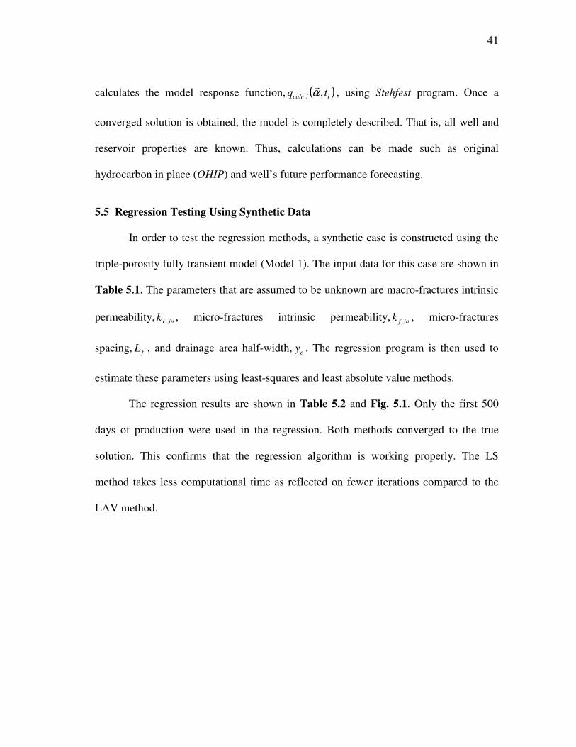
5.5 Regression Testing Using Synthetic Data .................................... 41

5.6 Regression Testing Using Simulated Data ................................... 43

5.7 Matching Noisy Data ................................................................... 45

5.8 Matching Gas Wells Rate ............................................................. 46

5.9 Notes on Regression Matching .................................................... 47

VI APPLICATION OF THE TRIPLE-POROSITY TO SHALE GAS

WELLS ................................................................................................. 48

6.1 Introduction .................................................................................. 48

6.2 Accounting for Adsorbed Gas ...................................................... 50

6.3 Analysis Procedure ....................................................................... 51

6.4 Field Cases ................................................................................... 52

ix

CHAPTER Page

6.4.1 Well 314 ............................................................................. 53

6.4.2 Well 73 ............................................................................... 56

6.5 Effect of Outer Reservoir ............................................................. 58

6.6 Chapter Summary ......................................................................... 61

VII CONCLUSIONS AND RECOMMENDATIONS ............................... 62

7.1 Conclusions .................................................................................. 62

7.2 Recommendations for Future Work ............................................. 63

NOMENCLATURE .................................................................................................. 64

REFERENCES .......................................................................................................... 67

APPENDIX A LINEAR FLOW SOLUTIONS FOR FRACTURED LINEAR

RESERVOIRS ............................................................................... 71

APPENDIX B DERIVATION OF LINEAR TRIPLE-POROSITY

ANALYTICAL SOLUTION FOR FULLY TRANSIENT

FLUID TRANSFER – MODEL 1 ................................................. 75

APPENDIX C DERIVATION OF LINEAR TRIPLE-POROSITY

ANALYTICAL SOLUTION FOR MODEL 2 .............................. 85

APPENDIX D DERIVATION OF LINEAR TRIPLE-POROSITY

ANALYTICAL SOLUTION FOR MODEL 3 .............................. 89

APPENDIX E DERIVATION OF LINEAR TRIPLE-POROSITY

ANALYTICAL SOLUTION FOR FULLY PSEUDOSTEADY

STATE FLUID TRANSFER– MODEL 4 ..................................... 93

APPENDIX F EFFECTS OF TRIPLE-POROSITY PARAMETERS ON

MODEL 1 RESPONSE .................................................................. 97

APPENDIX G SUMMARY OF SOLUTIONS ...................................................... 101

VITA ......................................................................................................................... 104

x

LIST OF FIGURES

FIGURE Page

2.1 Idealization of the heterogeneous porous medium (Warren & Root 1963) 5

2.2 Idealization of the heterogeneous porous medium (Kazemi 1969) ............ 6

3.1 Top view of a horizontal well in a triple-porosity system with sequential

flow. Arrows indicate flow directions ....................................................... 13

3.2 Sub-models of the triple-porosity model based on different interporosity

flow condition assumptions. PSS: pseudosteady state. USS: unsteady

state or transient. Arrows indicate flow directions .................................... 14

3.3 Comparison of the constant pressure solutions based on the four triple-

porosity models ......................................................................................... 21

3.4 A log-log plot of transient dual-porosity (DP) and triple-porosity (TP)

Models 1 and 2 solutions for constant pressure case. The two solutions

are identical indicating the mathematical consistency of the new triple-

porosity solutions ....................................................................................... 22

3.5 A log-log plot of pseudosteady state dual-porosity (DP) and triple-

porosity (TP) Models 3 and 4 solutions for constant pressure case. The

two solutions are matching indicating the mathematical consistency of

the new triple-porosity solutions . .............................................................. 23

3.6 A log-log plot of triple-porosity solution. Six flow regions can be

identified for Model 1 constant pressure solution. Slopes are labeled on

the graph .................................................................................................... 24

3.7 Log-log plot of dual-porosity and triple-porosity constant pressure

solutions for radial flow ............................................................................ 27

4.1 Top view of the CMG triple-porosity simulation model ........................... 31

4.2 Match between simulation and analytical solution results for the oil case.

(kF,in = 1000 md, kf,in = 1 md and km = 1.5×10-4

md) ................................. 32

4.3 Simulation and analytical solution match for the gas case. The boundary

dominated flow was matched very well after correcting for changing gas

properties. (kF,in = 2 md, kf,in = 0.1 md and km = 1.5×10-4

md) .................. 32

xi

FIGURE Page

4.4 Simulation and analytical solutions match for the triple-porosity system

with high macro-fractures permeability .................................................... 33

4.5 Simulation and analytical solutions match for the triple-porosity system

with high micro-fractures and macro-fractures permeability .................... 34

5.1 Regression results for the synthetic case using LS method. LV method

results are identical and are not shown. The desired solution was

achieved although not all data were used in regression ............................ 43

5.2 Regression results for the simulated case using LS and LAV methods.

The match using both methods is almost identical. The solution was

obtained without including all data in regression ...................................... 45

5.3 Effect of correcting for gas properties on the matching gas flow case.

The boundary dominated flow was matched very well after this

modification .............................................................................................. 47

6.1 Dual-porosity models for shale gas horizontal wells: slab model on the

left and cube model on the right (Al-Ahmadi et al. 2010) ........................ 49

6.2 Log-Log plot of gas rate versus time for two horizontal shale gas wells.

Well 314 exhibits a linear flow for almost two log cycles while Well 73

exhibit generally lower rate with bi-linear flow for early data and

changed to linear flow at later time. The blue and green lines indicate a

half-slope and a quarter-slope, respectively. .............................................. 52

6.3 Regression results for Well 314. The left plot does not include gas

adsorption while the right plot does. In both cases, the well’s data was

match using 500 days of production history .............................................. 55

6.4 Matching Well 314 production history using the regression results with

(bottom) and without (top) adsorption. On the left is the decline curve

plot and log-log plot is on the right for gas rate vs. time. .......................... 56

6.5 Regression match for Well 73 where it described the well trend perfectly

with (bottom) and without (top) gas adsorption. No good match was

obtained unless the whole data is used in the regression. On the left is

the decline curve plot and log-log plot is on the right for gas rate vs.

time. ............................................................................................................ 58

6.6 A sketch of the outer reservoir considered in the simulation model ......... 59

xii

FIGURE Page

6.7 Comparison of a gas well rate showing the effect of outer reservoir. The

outer reservoir effect is significant after four years of production for this

set of data. Only free gas is considered for this case .................................. 60

A-1 A sketch of a horizontal well in a rectangular reservoir. Linear flow is

the main flow regime. ................................................................................. 72

B-1 A sketch of triple-porosity system under sequential feed assumption.

Arrows show flow directions .................................................................... 75

F-1 Model 1 constant pressure solution: base case .......................................... 97

F-2 Effect of ωF on Model 1 constant pressure solution ................................. 98

F-3 Effect of ωf on Model 1 constant pressure solution .................................. 98

F-4 Effect of λAc,Ff on Model 1 constant pressure solution .............................. 99

F-5 Effect of λAc,fm on Model 1 constant pressure solution .............................. 99

F-6 Effect of yeD on Model 1 constant pressure solution ................................. 100

xiii

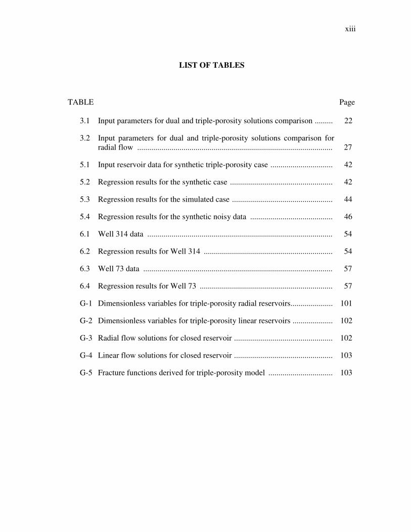
LIST OF TABLES

TABLE Page

3.1 Input parameters for dual and triple-porosity solutions comparison ......... 22

3.2 Input parameters for dual and triple-porosity solutions comparison for

radial flow ................................................................................................. 27

5.1 Input reservoir data for synthetic triple-porosity case ............................... 42

5.2 Regression results for the synthetic case ................................................... 42

5.3 Regression results for the simulated case .................................................. 44

5.4 Regression results for the synthetic noisy data ......................................... 46

6.1 Well 314 data ............................................................................................ 54

6.2 Regression results for Well 314 ................................................................ 54

6.3 Well 73 data .............................................................................................. 57

6.4 Regression results for Well 73 .................................................................. 57

G-1 Dimensionless variables for triple-porosity radial reservoirs..................... 101

G-2 Dimensionless variables for triple-porosity linear reservoirs .................... 102

G-3 Radial flow solutions for closed reservoir ................................................. 102

G-4 Linear flow solutions for closed reservoir ................................................. 103

G-5 Fracture functions derived for triple-porosity model ................................ 103

1

CHAPTER I

INTRODUCTION

A naturally fractured reservoir can be defined as a reservoir that contains a

connected network of fractures created by natural processes that have or predicted to

have an effect on the fluid flow (Nelson 2001). Naturally fractured reservoirs (NFRs)

contain more than 20% of the World’s hydrocarbon reserves (Sarma and Aziz 2006).

Moreover, most of the unconventional resources such as shale gas are also contained in

fractured reservoirs. Horizontal wells are becoming the norm for field development

nowadays. In addition, nearly all horizontal wells completed in shale and tight gas

reservoirs are hydraulically fractured.

Traditionally, dual-porosity models have been used to model NFRs where all

fractures are assumed to have identical properties. Many dual-porosity models have been

developed starting by Warren & Root (1963) sugar cube model in which matrix provides

the storage while fractures provide the flow medium. The model assumed pseudosteady

state fluid transfer between matrix and fractures. Since then several models were

developed mainly as variation of the Warren & Root model assuming different matrix-

fracture fluid transfer conditions.

____________

This thesis follows the style of SPE Reservoir Evaluation & Engineering.

2

However, it is more realistic to assume fractures having different properties. This

is more apparent in case of hydraulically fractured wells. Thus, triple-porosity models

have been developed as more realistic models to capture reservoir heterogeneity in

NFRs. Models for more than three interacting media are also available in the literature.

However, no triple-porosity model has been developed for linear flow in fractured

reservoirs. In addition, no triple-porosity (dual fracture) model is available for either

linear or radial flow that considers transient fluid transfer between matrix and micro-

fractures.

1.1 Motivation

The motivation behind this research was triggered by the Barnett Shale where

hydraulically fractured horizontal wells are drilled parallel to the pre-existing natural

fractures. It has been documented that hydraulic fractures growth could re-open the pre-

existing natural fractures (Gale et al. 2007). Therefore, for any model to be used to

analyze such wells, it has to account for both natural and hydraulic fractures to be

practical.

1.2 Objectives

The objective of this research is to develop analytical solutions to model the fluid

flow toward a horizontal well in a triple-porosity reservoir consisting of matrix and two

sets of orthogonal fractures that have different properties. These fractures are the more

permeable macro-fractures and the less permeable micro-fractures. El-Banbi (1998)

linear flow solutions will be used and new fracture functions will be derived.

3

1.3 Organization of the Thesis

This thesis is divided into seven chapters. The organization of these chapters is as

follows:

Chapter I is an introduction to the subject of this research, its motivations and

objectives.

Chapter II is devoted for literature review about modeling of fractured reservoirs

using dual, triple and multiple-porosity models with emphasis on linear flow.

Chapter III presents the new analytical triple-porosity solutions developed for

linear flow towards a horizontal well in triple-porosity reservoirs. The solutions are

verified for their mathematical consistency by comparing them with their dual-porosity

counterparts. In addition, the applicability of these solutions to radial systems and gas

flow are presented.

Chapter IV confirms the analytical solutions by numerical simulation model built

using CMG reservoir simulator.

Chapter V presents the non-linear regression as a tool to match field data using

the triple-porosity model. Two regression methods are presented: the least squares and

the least absolute value.

Chapter VI presents the application of the new model to shale gas horizontal

wells. The model uses non-linear regression to match the field data and estimate

reservoir parameters.

Chapter VII presents conclusions and recommendations.

4

CHAPTER II

LITERATURE REVIEW

This chapter provides a literature review of the NFRs modeling. Some of the

available dual, triple and multiple-porosity models will be reviewed. In addition, linear

flow solutions for fractured reservoirs will be discussed

2.1 Dual-porosity Models

Naturally fractured reservoirs are usually characterized using dual-porosity

models. The foundations of dual-porosity models were first introduced by Barenblatt et

al. (1960). The model assumes pseudosteady state fluid transfer between matrix and

fractures. Later, Warren and Root (1963) extended Barenblatt et al. model to well test

analysis and introduced it to the petroleum literature. The Warren & Root model was

mainly developed for transient well test analysis in which they introduced two

dimensionless parameters, ω and λ. ω describes the storativity of the fractures system

and λ is the parameter governing fracture-matrix flow.

Dual-porosity models can be categorized into two major categories based on the

interporosity fluid transfer assumption: pseudosteady state models and unsteady state

models.

2.1.1 Pseudosteady State Models

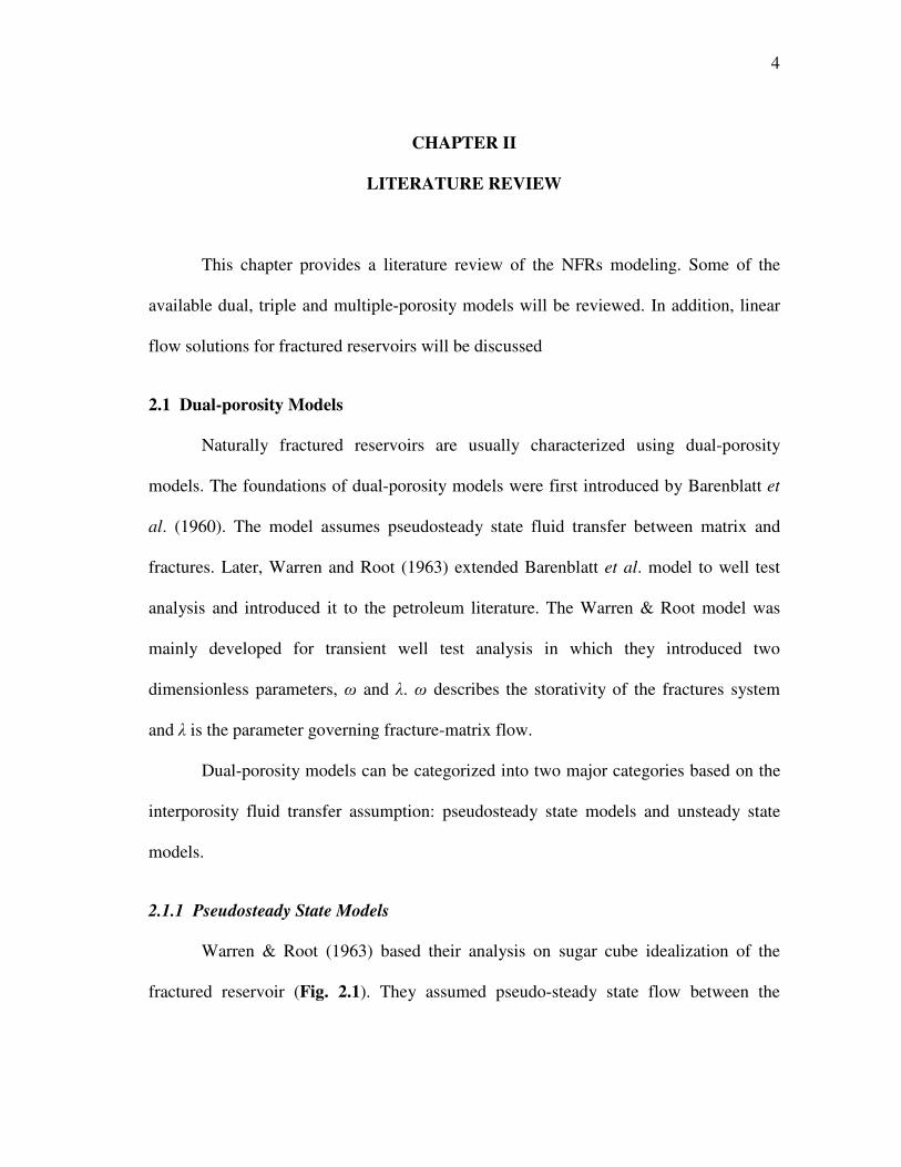
Warren & Root (1963) based their analysis on sugar cube idealization of the

fractured reservoir (Fig. 2.1). They assumed pseudo-steady state flow between the

5

matrix and fracture systems. That is, the pressure at the middle of the matrix block starts

changing at time zero. In their model, two differential forms (one for matrix and one for

fracture) of diffusivity equations were solved simultaneously at a mathematical point.

The fracture-matrix interaction is related by

( )fmm pp

kq −=

µα ........................................................................................ (2.1)

where q is the transfer rate, α is the shape factor, km is the matrix permeability, µ is the

fluid viscosity and (pm – pf) is the pressure difference between the matrix and the

fracture.

Fig. 2.1 – Idealization of the heterogeneous porous medium (Warren & Root 1963).

2.1.2 Unsteady State Models

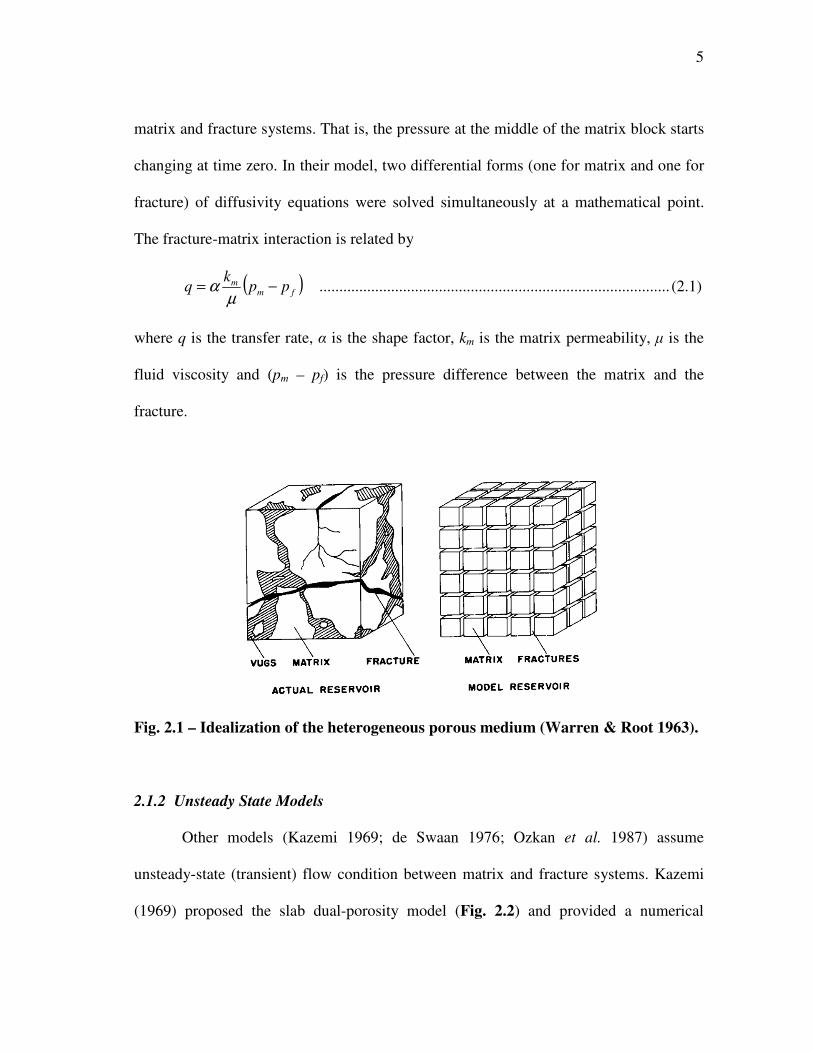
Other models (Kazemi 1969; de Swaan 1976; Ozkan et al. 1987) assume

unsteady-state (transient) flow condition between matrix and fracture systems. Kazemi

(1969) proposed the slab dual-porosity model (Fig. 2.2) and provided a numerical

6

solution for dual-porosity reservoirs assuming transient flow between matrix and

fractures. His solution, however, was similar to that of Warren & Root except for the

transition period between the matrix and fractures systems.

Fig. 2.2 – Idealization of the heterogeneous porous medium (Kazemi 1969).

2.2 Triple-porosity Models

The dual-porosity models assume uniform matrix and fractures properties

throughout the reservoir which may not be true in actual reservoirs. An improvement to

this drawback is to consider two matrix systems with different properties. This system is

a triple-porosity system. Another form of triple-porosity is to consider two fractures

systems with different properties in addition to the matrix. The latter is sometimes

referred to as dual fracture model.

The first triple-porosity model was developed by Liu (1981, 1983). Liu

developed his model for radial flow of slightly compressible fluids through a triple-

porosity reservoir under pseudosteady state interporosity flow. The idealization

Warren &

Root Model

Kazemi Model

7

considers two matrix systems flowing to a single fracture. Asymptotic cases were

considered where triple-porosity medium reduces to a single or dual porosity media.

This model, however, is rarely referenced as it was not published in the petroleum

literature.

In petroleum literature, however, the first triple-porosity model was introduced

by Abdassah and Ershaghi (1986). Two geometrical configurations were considered:

strata model and uniformly distributed blocks model. In both models, two matrix

systems have different properties flowing to a single fracture under gradient (unsteady

state) interporosity flow. The solutions were developed for radial system.

Jalali and Ershaghi (1987) investigated the transition zone behavior of the radial

triple porosity system. They extended the Abdassah and Ershaghi strata (layered) model

by allowing the matrix systems to have different properties and thickness. In addition,

three interporosity flow conditions were considered:

a. both matrix systems obey pseudosteady state flow

b. both matrix systems obey unsteady state flow

c. one matrix obeys pseudosteady state while the other obeys unsteady state

flow.

Al-Ghamdi and Ershaghi (1996) was the first to introduce the dual fracture triple-

porosity model for radial system. Their model consists of a matrix and two fracture

systems; more permeable macro-fracture and less permeable micro-fracture. Two sub

models were presented. The first is similar to the triple-porosity layered model where

micro-fractures replace one of the matrix systems. The second is where the matrix feeds

8

the micro-fractures under pseudosteady state flow which in turns feed the macro-

fractures under pseudosteady state flow condition as well. The macro-fractures and/or

micro-fractures are allowed to flow to the well.

Liu et al. (2003) presented a radial triple-continuum model. The system consists

of fractures, matrix and cavity media. Only the fractures feed the well but they receive

flow from both matrix and cavity systems under pseudosteady state condition. Unlike

previous triple-porosity models, the matrix and cavity systems are exchanging flow

(under pseudosteady state condition) and thus it is called triple-continuum. Their

solution was an extension of Warren and Root solution.

Wu et al. (2004) used the triple-continuum model for modeling flow and

transport of tracers and nuclear waste in the unsaturated zone of Yucca Mountain. The

system consists of large fractures, small fractures and matrix. They confirmed the

validity of the analytical solution with numerical simulation for injection well injecting

at constant rate in a radial system. In addition, they demonstrated the usefulness of the

triple-continuum model for estimating reservoir parameters.

Dreier (2004) improved the triple-porosity dual fracture model originally

developed by Al-Ghamdi and Ershaghi (1996) by considering transient flow condition

between micro-fractures and macro-fractures. Flow between matrix and micro-fractures

is still under pseudosteady state condition. His main work (Dreier et al. 2004) was the

development of new quadruple-porosity sequential feed and simultaneous feed models.

He addressed the need for nonlinear regression to match well test data and estimate

reservoir properties in case of quadruple porosity model. For the triple-porosity dual

9

fracture model, the solution was derived in Laplace domain for radial system for a

constant rate case with the following fracture function:

( ) ( ) ( )( )

( )

+⋅⋅+⋅⋅⋅=

⋅⋅⋅⋅⋅+=

λω

λωωκ

κ

sshsf

sfsfhhs

sf

m

mfrmDfr

frfr

frDmD

3

2

,3

33

2,,

tanh1111

1

...................................... (2.2)

The dimensionless variables definitions they used are different from these used in this

work.

2.3 Linear Flow in Fractured Reservoirs

Linear flow occurs at early time (transient flow) when flow is perpendicular to

any flow surface. Wattenbarger (2007) identified different causes for linear transient

flow including hydraulic fracture draining a square geometry, high permeability layers

draining adjacent tight layers and early-time constant pressure drainage from different

geometries.

El-Banbi (1998) developed new linear dual-porosity solutions for fluid flow in

linear fractured reservoirs. Solutions were derived in Laplace domain for several inner

and outer boundary conditions. These include constant rate and constant pressure inner

boundaries and infinite and closed outer boundaries. Skin and wellbore storage effects

have been incorporated as well. One important finding is that reservoir functions, ( )sf ,

derived for radial flow can be used in linear flow solutions in Laplace domain and vice

versa.

10

Bello (2009) demonstrated that El-Banbi solutions could be used to model

horizontal well performance in tight fractured reservoirs. He then applied the constant

pressure solution to analyze rate transient in horizontal multi-stage fractured shale gas

wells.

Bello (2009) and Bello and Wattenbarger (2008, 2009, 2010) used the dual-

porosity linear flow model to analyze shale gas wells. Five flow regions were defined

based on the linear dual-porosity constant pressure solution. It was found that shale gas

wells performance could be analyzed effectively by region 4 (transient linear flow from

a homogeneous matrix). Skin effect was proposed to affect the early flow periods and a

modified algebraic equation was proposed to account for it.

Ozkan et al. (2009) and Brown et al. (2009) proposed a tri-linear model for

analyzing well test in tight gas wells. Three contiguous media were considered: finite

conductivity hydraulic fractures, dual-porosity inner reservoir between the hydraulic

fractures and outer reservoir beyond the tip of the hydraulic fractures. Based on their

analysis, the outer reservoir does not contribute significantly to the flow.

Al-Ahmadi et al. (2010) presented procedures to analyze shale gas wells using

the slab and cube dual-porosity idealizations demonstrated by field examples.

11

CHAPTER III

TRIPLE-POROSITY MODEL FOR FRACTURED RESERVOIRS: NEW

SOLUTIONS

3.1 Introduction

In this chapter, a triple-porosity model is developed and new solutions are

derived for linear flow in fractured reservoirs. The triple-porosity system consists of

three contiguous porous media: the matrix, less permeable micro-fractures and more

permeable macro-fractures. The main flow is through the macro-fractures which feed the

well while they receive flow from the micro-fractures only. Consequently, the matrix

feeds the micro-fractures only. Therefore, the flow is sequential from one medium to the

other. In the petroleum literature, this type of model is sometimes called dual-fracture

model.

The problem at hand is to model the fluid flow toward a horizontal well in a

triple-porosity reservoir. El-Banbi (1998) solutions for linear flow in dual-porosity

reservoirs will be used. However, new reservoir functions will be derived that pertain to

the triple-porosity system and can be used in El-Banbi’s solutions.

Throughout this thesis, matrix, micro-fractures and macro-fractures are identified

with subscripts m, f and F, respectively.

12

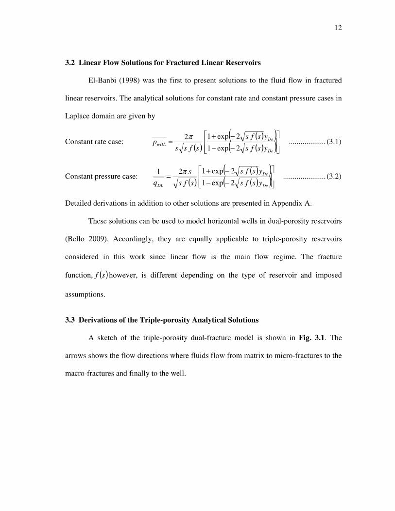
3.2 Linear Flow Solutions for Fractured Linear Reservoirs

El-Banbi (1998) was the first to present solutions to the fluid flow in fractured

linear reservoirs. The analytical solutions for constant rate and constant pressure cases in

Laplace domain are given by

Constant rate case: ( )

( )( )( )( )

−−

−+=

De

De

wDLysfs

ysfs

sfssp

2exp1

2exp12π ................... (3.1)

Constant pressure case: ( )

( )( )( )( )

−−

−+=

De

De

DL ysfs

ysfs

sfs

s

q 2exp1

2exp121 π ...................... (3.2)

Detailed derivations in addition to other solutions are presented in Appendix A.

These solutions can be used to model horizontal wells in dual-porosity reservoirs

(Bello 2009). Accordingly, they are equally applicable to triple-porosity reservoirs

considered in this work since linear flow is the main flow regime. The fracture

function, ( )sf however, is different depending on the type of reservoir and imposed

assumptions.

3.3 Derivations of the Triple-porosity Analytical Solutions

A sketch of the triple-porosity dual-fracture model is shown in Fig. 3.1. The

arrows shows the flow directions where fluids flow from matrix to micro-fractures to the

macro-fractures and finally to the well.

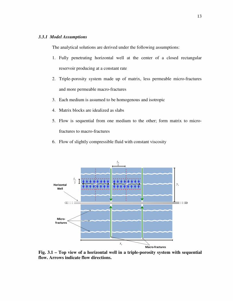
13

3.3.1 Model Assumptions

The analytical solutions are derived under the following assumptions:

1. Fully penetrating horizontal well at the center of a closed rectangular

reservoir producing at a constant rate

2. Triple-porosity system made up of matrix, less permeable micro-fractures

and more permeable macro-fractures

3. Each medium is assumed to be homogenous and isotropic

4. Matrix blocks are idealized as slabs

5. Flow is sequential from one medium to the other; form matrix to micro-

fractures to macro-fractures

6. Flow of slightly compressible fluid with constant viscosity

2

fL

ex

ey

Micro-

fractures

Macro-fractures

Horizontal

Well

2

FL

Fig. 3.1 – Top view of a horizontal well in a triple-porosity system with sequential

flow. Arrows indicate flow directions.

14

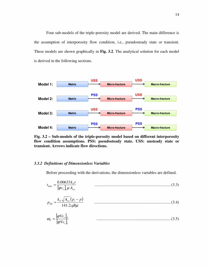
Four sub-models of the triple-porosity model are derived. The main difference is

the assumption of interporosity flow condition, i.e., pseudosteady state or transient.

These models are shown graphically in Fig. 3.2. The analytical solution for each model

is derived in the following sections.

Macro-fractureMatrix Micro-fracture

USS USS


PSS USS


USS PSS


PSS PSS

Model 1:

Model 2:

Model 3:

Model 4:

Fig. 3.2 – Sub-models of the triple-porosity model based on different interporosity

flow condition assumptions. PSS: pseudosteady state. USS: unsteady state or

transient. Arrows indicate flow directions.

3.3.2 Definitions of Dimensionless Variables

Before proceeding with the derivations, the dimensionless variables are defined.

[ ] cwtt

FDAc

Ac

tkt

µϕ

00633.0= ........................................................................... (3.3)

( )µqB

ppAkp

icwF

DL2.141

−= ........................................................................... (3.4)

[ ][ ]

tt

Ft

FVc

Vc

ϕ

ϕω = ......................................................................... (3.5)

15

[ ][ ]

tt

ft

fVc

Vc

ϕ

ϕω = ........................................................................ (3.6)

[ ][ ] fF

tt

mt

mVc

Vcωω

ϕ

ϕω −−== 1 ......................................................................... (3.7)

cw

F

f

F

FfAc Ak

k

L2,

12=λ ........................................................................... (3.8)

cw

F

m

f

fmAc Ak

k

L2,

12=λ .......................................................................... (3.9)

2fLD

zz = ......................................................................... (3.10)

2FLD

xx = ......................................................................... (3.11)

cw

DA

yy = ........................................................................ (3.12)

ω and λ are the storativity ratio and interporosity flow parameter, respectively. kF

and kf are the bulk (macroscopic) fractures permeabilities

3.3.3 Model 1: Fully Transient Triple-porosity Model

The first sub-model, Model 1, is the fully transient model. The flow between

matrix and micro-fractures and that between micro-fractures and macro-fractures are

under transient condition. This model is an extension to the dual-porosity transient slab

model (Kazemi 1969 Model). The derivation starts by writing the differential equations

describing the flow in each medium.

16

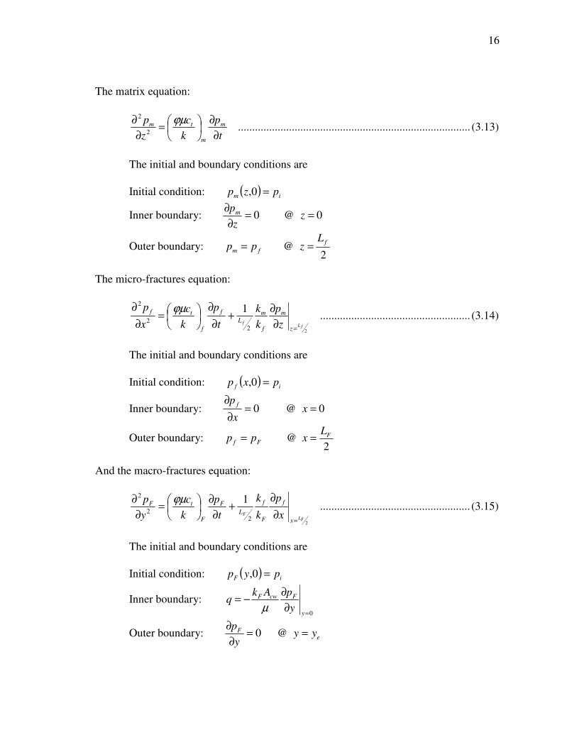
The matrix equation:

t

p

k

c

z

p m

m

tm

∂

∂

=

∂

∂ ϕµ2

2

.................................................................................. (3.13)

The initial and boundary conditions are

Initial condition: ( ) im pzp =0,

Inner boundary: 0@0 ==∂

∂z

z

pm

Outer boundary: 2

@f

fm

Lzpp ==

The micro-fractures equation:

22

2

21

fLf

z

m

f

m

L

f

f

tf

z

p

k

k

t

p

k

c

x

p

=∂

∂+

∂

∂

=

∂

∂ ϕµ ..................................................... (3.14)


Initial condition: ( )if pxp =0,


∂x

x

p f

Outer boundary: 2

@ FFf

Lxpp ==

And the macro-fractures equation:

22

2

2 1

FLF

x

f

F

f

L

F

F

tF

x

p

k

k

t

p

k

c

y

p

=∂

∂+

∂

∂

=

∂

∂ ϕµ ..................................................... (3.15)


Initial condition: ( ) iF pyp =0,

Inner boundary: 0=

∂

∂−=

y

FcwF

y

pAkq

µ

Outer boundary: eF yyy

p==

∂

∂@0

17

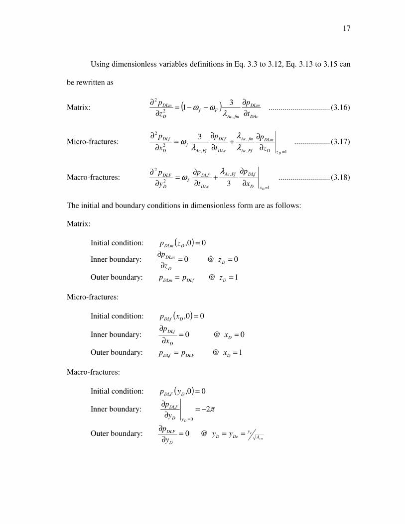
Using dimensionless variables definitions in Eq. 3.3 to 3.12, Eq. 3.13 to 3.15 can

be rewritten as

Matrix: ( )DAc

DLm

fmAc

Ff

D

DLm

t

p

z

p

∂

∂−−=

∂

∂

,

2

2 31

λωω ............................... (3.16)

Micro-fractures:

1,

,

,

2

23

=∂

∂+

∂

∂=

∂

∂

DzD

DLm

FfAc

fmAc

DAc

DLf

FfAc

f

D

DLf

z

p

t

p

x

p

λ

λ

λω .................. (3.17)

Macro-fractures:

1

,

2

2

3=

∂

∂+

∂

∂=

∂

∂

DxD

DLfFfAc

DAc

DLFF

D

DLF

x

p

t

p

y

p λω .......................... (3.18)

The initial and boundary conditions in dimensionless form are as follows:

Matrix:

Initial condition: ( ) 00, =DDLm zp


∂D

D

DLm zz

p

Outer boundary: 1@ == DDLfDLm zpp

Micro-fractures:

Initial condition: ( ) 00, =DDLf xp


∂D

D

DLfx

x

p

Outer boundary: 1@ == DDLFDLf xpp

Macro-fractures:

Initial condition: ( ) 00, =DDLF yp

Inner boundary: π2

0

−=∂

∂

=DyD

DLF

y

p

Outer boundary: cw

e

A

yDeD

D

DLF yyy

p===

∂

∂@0

18

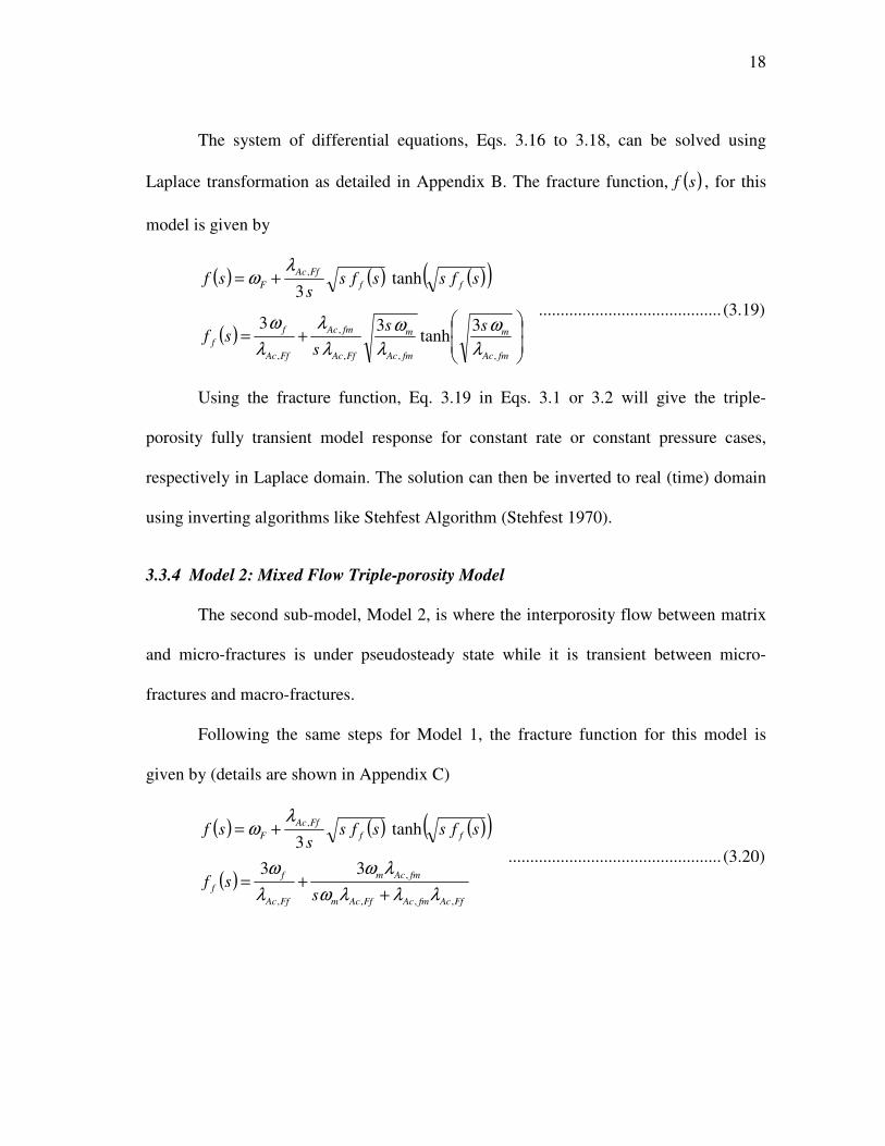
The system of differential equations, Eqs. 3.16 to 3.18, can be solved using

Laplace transformation as detailed in Appendix B. The fracture function, ( )sf , for this

model is given by

( ) ( ) ( )( )

( )

+=

+=

fmAc

m

fmAc

m

FfAc

fmAc

FfAc

f

f

ff

FfAc

F

ss

ssf

sfssfss

sf

,,,

,

,

,

3tanh

33

tanh3

λ

ω

λ

ω

λ

λ

λ

ω

λω

.......................................... (3.19)

Using the fracture function, Eq. 3.19 in Eqs. 3.1 or 3.2 will give the triple-

porosity fully transient model response for constant rate or constant pressure cases,

respectively in Laplace domain. The solution can then be inverted to real (time) domain

using inverting algorithms like Stehfest Algorithm (Stehfest 1970).

3.3.4 Model 2: Mixed Flow Triple-porosity Model

The second sub-model, Model 2, is where the interporosity flow between matrix

and micro-fractures is under pseudosteady state while it is transient between micro-

fractures and macro-fractures.

Following the same steps for Model 1, the fracture function for this model is

given by (details are shown in Appendix C)

( ) ( ) ( )( )

( )FfAcfmAcFfAcm

fmAcm

FfAc

f

f

ff

FfAc

F

ssf

sfssfss

sf

,,,

,

,

,

33

tanh3

λλλω

λω

λ

ω

λω

++=

+=

................................................. (3.20)

19

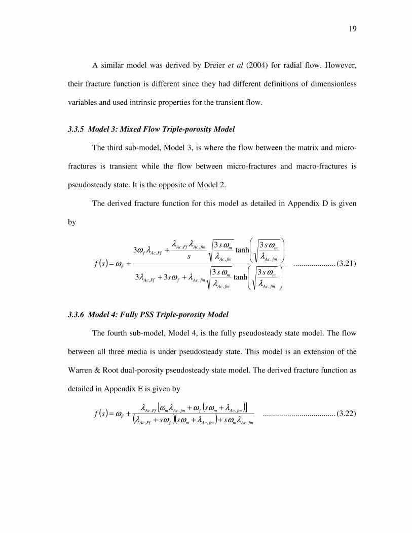
A similar model was derived by Dreier et al (2004) for radial flow. However,

their fracture function is different since they had different definitions of dimensionless

variables and used intrinsic properties for the transient flow.

3.3.5 Model 3: Mixed Flow Triple-porosity Model

The third sub-model, Model 3, is where the flow between the matrix and micro-

fractures is transient while the flow between micro-fractures and macro-fractures is

pseudosteady state. It is the opposite of Model 2.

The derived fracture function for this model as detailed in Appendix D is given

by

( )

++

+

+=

fmAc

m

fmAc

mfmAcfFfAc

fmAc

m

fmAc

mfmAcFfAc

FfAcf

F

sss

ss

ssf

,,

,,

,,

,,

,

3tanh

333

3tanh

33

λ

ω

λ

ωλωλ

λ

ω

λ

ωλλλω

ω ..................... (3.21)

3.3.6 Model 4: Fully PSS Triple-porosity Model

The fourth sub-model, Model 4, is the fully pseudosteady state model. The flow

between all three media is under pseudosteady state. This model is an extension of the

Warren & Root dual-porosity pseudosteady state model. The derived fracture function as

detailed in Appendix E is given by

( )( )[ ]

( )( )fmAcmfmAcmfFfAc

fmAcmffmAcmFfAc

Fsss

ssf

,,,

,,,

λωλωωλ

λωωλωλω

+++

+++= .................................... (3.22)

20

This model is also a limiting case of Liu et al (2000; Wu et al, 2004) triple-

continuum model if considering sequential flow and ignoring the flow component

between matrix and macro-fractures.

3.3.7 Triple-porosity Solutions Comparison

Models 1 through 4 cover all possibilities of fluid flow in triple-porosity system

under sequential flow assumption. Comparison of the constant pressure solution based

on these models is shown in Fig. 3.3. As can be seen on the figure, Models 1 and 4

represents the end members while Models 2 and 3 are combination of these models.

Model 2 follows Model 1 at early time but follows Model 4 at later time while Model 3

is the opposite.

Considering rate transient analysis, Models 1 and 3 are more likely to be

applicable to field data.

21

1.E-09

1.E-08

1.E-07

1.E-06

1.E-05

1.E-04

1.E-03

1.E-02

1.E-01

1.E+00

1.E+01

1.E+02

1.E+03

1.E

-15

1.E

-14

1.E

-13

1.E

-12

1.E

-11

1.E

-10

1.E

-09

1.E

-08

1.E

-07

1.E

-06

1.E

-05

1.E

-04

1.E

-03

1.E

-02

1.E

-01

1.E

+00

1.E

+01

1.E

+02

1.E

+03

1.E

+04

1.E

+05

1.E

+06

1.E

+07

qD

L

tDAc

Model 1: Fully Trasient

Model 4: Fully PSS

Model 2: Mixed Flow (Trasient - PSS)

Model 3: Mixed Flow (PSS - Transient)

Fig. 3.3 – Comparison of the constant pressure solutions based on the four triple-

porosity models.

3.4 Mathematical Consistency of the Analytical Solutions

In this section, the solutions mathematical consistency is checked by reducing the

triple-porosity model to its dual-porosity counterpart. This can be achieved by allowing

the micro-fractures to dominate the flow and assigning to them the dual-porosity matrix

properties from the dual-porosity system. In this case, the matrix-micro-fractures

interporosity coefficient, fmAc,λ , is very small and the triple-porosity matrix storativity

ratio, ω, is zero. This comparison is shown for all models in the following figures. Table

3.1 shows the data used for comparison.

22

Table 3.1 – Input parameters for dual and triple-porosity

solutions comparison

Dual-Porosity Parameters Triple-Porosity Parameters

ω 0.001 ωF 0.001

λ 0.005 ωf 0.999

yeD 10 λAc,Ff 0.005

λAc,fm 1×10-9

yeD 10

Models 1 and 2 are reduced to the transient slab dual-porosity model since the

flow between micro-fractures and macro-fractures is under transient conditions in the

two models. As shown Fig. 3.4, the triple-porosity solutions are identical to their dual-

porosity counterpart. This confirms the mathematical consistency of Models 1 and 2.

1.E-02

1.E-01

1.E+00

1.E+01

1.E+02

1.E+03

1.E+04

1.E+05

1.E+06

1.E+07

1.E

-07

1.E

-06

1.E

-05

1.E

-04

1.E

-03

1.E

-02

1.E

-01

1.E

+0

0

1.E

+0

1

1.E

+0

2

1.E

+0

3

1.E

+0

4

1/q

DL

, (

1/q

DL)'

tDAc

1/qDL - Dual-Porosity (1/qDL)' - Dual-Porosity

1/qDL - Triple-Porosity Model 1 (1/qDL)' - Triple-Porosity Model 1


Fig. 3.4 –A log-log plot of transient dual-porosity (DP) and triple-porosity (TP)

Models 1 and 2 solutions for constant pressure case. The two solutions are identical

indicating the mathematical consistency of the new triple-porosity solutions.

23

Models 3 and 4, however, are reduced to the pseudosteady state dual-porosity

model since the flow between micro-fractures and macro-fractures is under

pseudosteady state condition in the two models. As shown in Fig. 3.5, the triple-porosity

solutions are identical to their dual-porosity counterpart. This confirms the mathematical

consistency of Models 3 and 4.

1.E-04

1.E-03

1.E-02

1.E-01

1.E+00

1.E+01

1.E+02

1.E+03

1.E+04

1.E+05

1.E+06

1.E+07

1.E+08

1.E

-07

1.E

-06

1.E

-05

1.E

-04

1.E

-03

1.E

-02

1.E

-01

1.E

+0

0

1.E

+0

1

1.E

+0

2

1.E

+0

3

1.E

+0

4

1/q

DL

, (

1/q

DL)'

tDAc

1/qDL - Dual-Porosity (1/qDL)' - Dual-Porosity



Fig. 3.5 – A log-log plot of pseudosteady state dual-porosity (DP) and triple-

porosity (TP) Models 3 and 4 solutions for constant pressure case. The two

solutions are matching indicating the mathematical consistency of the new triple-

porosity solutions.

3.5 Flow Regions Based on the Analytical Solution

Since Model 1, the fully transient model, is the most general of all the four triple-

porosity variations and shows all possible flow regions, all discussions in this section

and the following chapters will be limited to Model 1. Based on Model 1 constant

24

pressure solution, six flow regions can be identified as the pressure propagates through

the triple-porosity system. These flow regions are shown graphically on the log-log plot

of dimensionless rate versus dimensionless time in Fig 3.6. Regions 1 through 5 exhibit

an alternating slopes of – ½ and – ¼ indicating linear and bilinear transient flow,

respectively. Region 6 is the boundary dominated flow and exhibits an exponential

decline due to constant bottom-hole pressure. These flow regions are explained in details

in the following sections. Appendix F shows the effect of each solution parameter on

Model 1 response for constant pressure case.

1.E-09

1.E-08

1.E-07

1.E-06

1.E-05

1.E-04

1.E-03

1.E-02

1.E-01

1.E+00

1.E+01

1.E+02

1.E+03

1.E

-15

1.E

-14

1.E

-13

1.E

-12

1.E

-11

1.E

-10

1.E

-09

1.E

-08

1.E

-07

1.E

-06

1.E

-05

1.E

-04

1.E

-03

1.E

-02

1.E

-01

1.E

+00

1.E

+01

1.E

+02

1.E

+03

1.E

+04

1.E

+05

1.E

+06

1.E

+07

qD

L

tDAcw

ωF 1.00E-07

ω f 1.00E-04

λFf 1.00E+02

λfm 1.00E-06

yeD 100

Region 1

Region 2

Region 3

Region 4

Region 5

Region 6

Half-Slope

Quarter-Slope

Fig. 3.6 – A log-log plot of triple-porosity solution. Six flow regions can be identified

for Model 1 constant pressure solution. Slopes are labeled on the graph.

25

3.5.1 Region 1

Region 1 represents the transient linear flow in the macro-fractures only. The

permeability of macro-fractures is usually high and hence, in most cases, this flow

region will be very short. It may not be captured by most well rate measurement tools.

This flow region exhibits a half-slope on the log-log plot of rate versus time.

3.5.2 Region 2

Region 2 is the bilinear flow in the macro-fractures and micro-fractures. It is

caused by simultaneous perpendicular transient linear flow in the micro-fractures and the

macro-fractures. This flow region exhibit a quarter-slope on the log-log plot of rate

versus time.

3.5.3 Region 3

Region 3 is the linear flow in the micro-fractures system. It will occur once the

transient flow in the macro-fractures ends indicating the end of bilinear flow (region 2).

This flow region exhibits a half-slope on the log-log plot of rate versus time.

3.5.4 Region 4

Region 4 is the bilinear flow in the micro-fractures and matrix. It is caused by the

linear flow in the matrix while the micro-fractures are still in transient flow. This flow

region exhibits a quarter-slope on the log-log plot of rate versus time. In most field

cases, this flow region is the first one to be observed.

26

3.5.5 Region 5

Region 5 is the main and longest flow region in most field cases. It is the linear

flow out of the matrix to the surrounding micro-fractures. This region exhibits a half-

slope on the log-log plot of rate versus time. Analysis of this region will allow the

estimation of fractures surface area available to flow, Acm.

3.5.6 Region 6

Region 6 is the boundary dominated flow. It starts when the pressure at the center

of the matrix blocks starts to decline. This flow is governed by exponential decline due

to constant bottom-hole pressure.

3.6 Triple-porosity Solutions for Radial Flow

Although the triple-porosity solutions were derived for linear flow, they are

equally applicable to radial flow following El-Banbi (1998) work. The differential

equation in Laplace domain that governs the flow in the macro-fractures in case of radial

system is given by

( ) 01

=−

∂

∂

∂

∂DF

D

DF

D

DD

psfsr

pr

rr ............................................................ (3.23)

The constant pressure solution for a closed reservoir is given by (El-Banbi 1998)

( )( ) ( )( ) ( )( ) ( )( )[ ]( ) ( )( ) ( )( ) ( )( ) ( )( )[ ]eDeD

eDeD

D rsfsKsfsIsfsKrsfsIsfs

sfsKrsfsIrsfsKsfsIs

q1111

01101

+

+= ..... (3.24)

The fractures functions, ( )sf , derived for all the models can be used in the radial

flow solutions as well. Fig. 3.7 shows comparison between radial dual-porosity solutions

27

and the new triple-porosity solutions reduced to their dual-porosity counterpart and

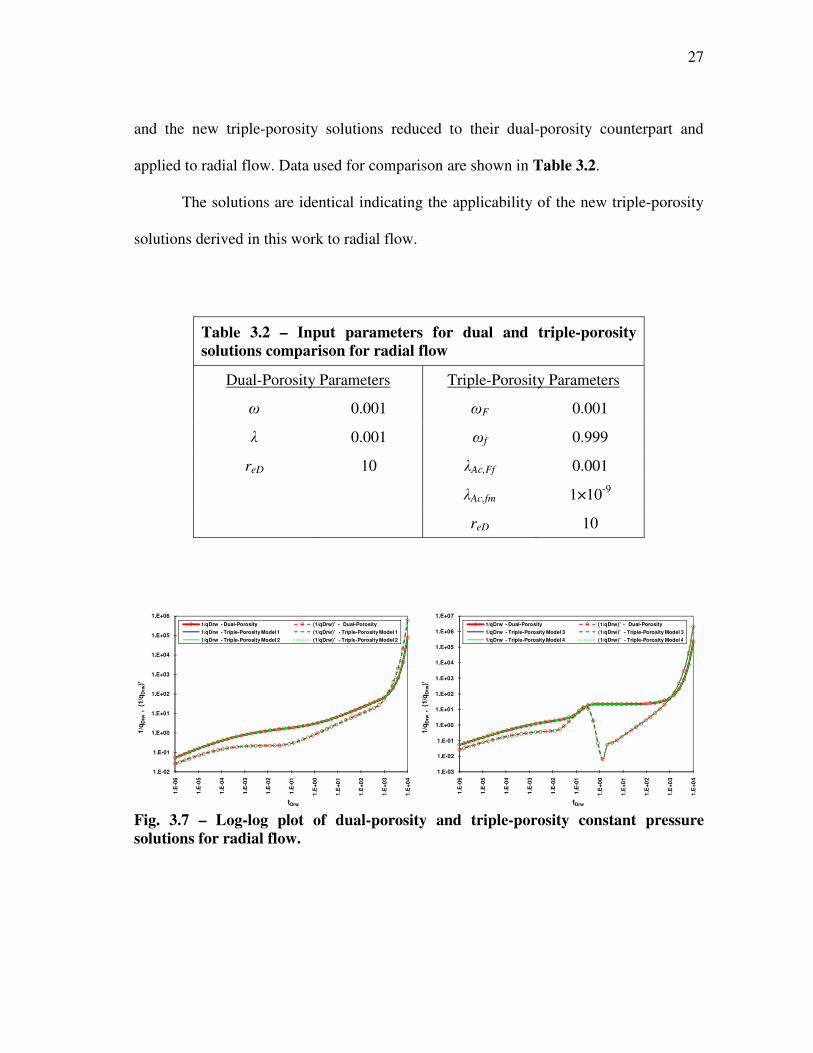
applied to radial flow. Data used for comparison are shown in Table 3.2.

The solutions are identical indicating the applicability of the new triple-porosity

solutions derived in this work to radial flow.

Table 3.2 – Input parameters for dual and triple-porosity

solutions comparison for radial flow

Dual-Porosity Parameters Triple-Porosity Parameters

ω 0.001 ωF 0.001

λ 0.001 ωf 0.999

reD 10 λAc,Ff 0.001

λAc,fm 1×10-9

reD 10

1.E-02

1.E-01

1.E+00

1.E+01

1.E+02

1.E+03

1.E+04

1.E+05

1.E+06

1.E

-06

1.E

-05

1.E

-04

1.E

-03

1.E

-02

1.E

-01

1.E

+0

0

1.E

+0

1

1.E

+0

2

1.E

+0

3

1.E

+0

4

1/q

Drw

, (

1/q

Drw

)'

tDrw

1/qDrw - Dual-Porosity (1/qDrw)' - Dual-Porosity

1/qDrw - Triple-Porosity Model 1 (1/qDrw)' - Triple-Porosity Model 1


1.E-03

1.E-02

1.E-01

1.E+00

1.E+01

1.E+02

1.E+03

1.E+04

1.E+05

1.E+06

1.E+07

1.E

-06

1.E

-05

1.E

-04

1.E

-03

1.E

-02

1.E

-01

1.E

+0

0

1.E

+0

1

1.E

+0

2

1.E

+0

3

1.E

+0

4

1/q

Drw

, (

1/q

Drw

)'

tDrw

1/qDrw - Dual-Porosity (1/qDrw)' - Dual-Porosity



Fig. 3.7 – Log-log plot of dual-porosity and triple-porosity constant pressure

solutions for radial flow.

28

3.7 Application to Gas Flow

It is important to note that the above solutions were derived for slightly

compressible fluids and thus are applicable to liquid flow only. However, they can be

applied to gas flow by using gas potential, ( )pm , instead of pressure to linearize the left-

hand side of the diffusivity equation. Therefore, the dimensionless pressure variable will

be defined in terms of gas potential as

( ) ( )[ ]Tq

pmpmAkm

g

icwF

DL1422

−= ...................................................................... (3.25)

where ( )pm is the gas potential defined as (Al-Hussainy et al. 1966)

( ) dpz

ppm

p

p

∫=

0

2µ

......................................................................................... (3.26)

With the above linearization, the derived solutions are applicable to the transient

flow regime for gas flow. However, once the reservoir boundaries are reached and

average reservoir pressure starts to decline, the gas properties will change considerably

especially the gas viscosity and compressibility. Therefore, the solutions have to be

corrected for changing fluid properties. This is usually achieved by using pseudo-time or

material balance time. An example of these transformations is the Fraim and

Wattenbarger (1987) normalized time defined as

( )( ) ( )

τµ

µd

pcp

ct

t

t

it

n ∫=0

...................................................................................... (3.27)

Thus, with these two modifications, the analytical solutions derived in this work

are applicable to gas flow.

29

3.8 Chapter Summary

In this chapter, four new triple-solutions have been developed to model the fluid

flow in a triple-porosity (dual-fracture) system under sequential flow assumption. Six

flow regions were identified based on this model. According to the best knowledge of

the author, the triple-porosity model for linear fractured reservoirs is new and has not

been presented in the literature before. In addition, even for radial reservoirs these

solutions are new and have not been presented before in this form.

30

CHAPTER IV

TRIPLE-POROSITY SIMULATION MODEL AND ANALYTICAL SOLUTIONS

VERIFICATION

4.1 Introduction

In this chapter, a triple-porosity simulation model is built using CMG reservoir

simulator. The objective is to understand the behavior of triple-porosity reservoirs and to

verify the analytical solutions derived in Chapter III.

The model considers the flow toward a horizontal well in a triple-porosity

reservoir. One representative segment is modeled which represents one quadrant of the

reservoir volume around a macro-fracture.

4.2 Simulation Model Description

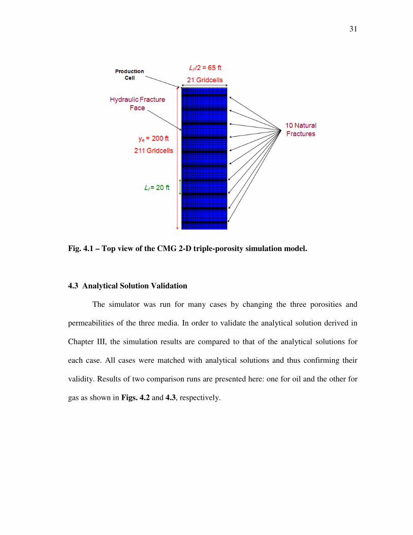
The model was built with the CMG reservoir simulator. Only one segment was

simulated representing one quadrant of the reservoir volume around one macro-fracture.

This segment contains ten micro-fractures orthogonal to the macro-fractures at 20 ft

fracture spacing. The model is a 2-D model with 21 gridcells in the x-direction, 211

gridcells in y-direction and only one cell in the z-direction. A top view of the model is

shown in Fig. 4.1. All matrix, micro-fractures and macro-fractures properties are

assigned explicitly. In addition, the simulation model assumes connate water saturation

for both oil and gas cases.

31

Fig. 4.1 – Top view of the CMG 2-D triple-porosity simulation model.

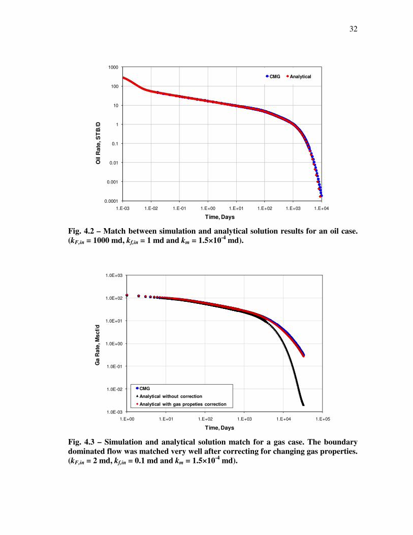
4.3 Analytical Solution Validation

The simulator was run for many cases by changing the three porosities and

permeabilities of the three media. In order to validate the analytical solution derived in

Chapter III, the simulation results are compared to that of the analytical solutions for

each case. All cases were matched with analytical solutions and thus confirming their

validity. Results of two comparison runs are presented here: one for oil and the other for

gas as shown in Figs. 4.2 and 4.3, respectively.

32

0.0001

0.001

0.01

0.1

1

10

100

1000

1.E-03 1.E-02 1.E-01 1.E+00 1.E+01 1.E+02 1.E+03 1.E+04

Oil R

ate

, S

TB

/D

Time, Days

CMG Analytical

Fig. 4.2 – Match between simulation and analytical solution results for an oil case.

(kF,in = 1000 md, kf,in = 1 md and km = 1.5×10-4

md).

1.0E-03

1.0E-02

1.0E-01

1.0E+00

1.0E+01

1.0E+02

1.0E+03

1.E+00 1.E+01 1.E+02 1.E+03 1.E+04 1.E+05

Ga

Ra

te, M

sc

f/d

Time, Days

CMG

Analytical without correction

Analytical with gas propeties correction

Fig. 4.3 – Simulation and analytical solution match for a gas case. The boundary

dominated flow was matched very well after correcting for changing gas properties.

(kF,in = 2 md, kf,in = 0.1 md and km = 1.5×10-4

md).

33

4.4 Limiting Cases

In order to confirm the integrity of the simulation model and the analytical

solution, asymptotic cases were run in which the triple-porosity system will reduce to a

simpler system, i.e., dual-porosity or homogenous system.

The first case is to assign a very high permeability to the macro-fractures. Thus,

the transient flow in the macro-fracture will be very fast and the system will act as if it is

dual-porosity system, i.e., the macro-fractures are effectively eliminated. The results are

shown in Fig. 4.4. The triple-porosity and dual-porosity solutions are matching the

simulation results. This indicates that the system can be effectively described by dual-

porosity model. In addition, the triple-porosity is matching the dual-porosity solution

indicating that the new solution is valid.

1.E-04

1.E-03

1.E-02

1.E-01

1.E+00

1.E+01

1.E+02

1.E+03

1.E+04

1.E-06 1.E-05 1.E-04 1.E-03 1.E-02 1.E-01 1.E+00 1.E+01 1.E+02 1.E+03 1.E+04

Oil R

ate

, S

TB

/D

Time, Days

Simulation - CMG

Analytical - Dual Porosity

Analytical - Triple Porosity

Fig. 4.4 – Simulation and analytical solutions match for the triple-porosity system

with high macro-fractures permeability.

34

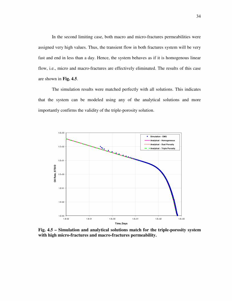
In the second limiting case, both macro and micro-fractures permeabilities were

assigned very high values. Thus, the transient flow in both fractures system will be very

fast and end in less than a day. Hence, the system behaves as if it is homogenous linear

flow, i.e., micro and macro-fractures are effectively eliminated. The results of this case

are shown in Fig. 4.5.

The simulation results were matched perfectly with all solutions. This indicates

that the system can be modeled using any of the analytical solutions and more

importantly confirms the validity of the triple-porosity solution.

1.E-03

1.E-02

1.E-01

1.E+00

1.E+01

1.E+02

1.E+03

1.E-02 1.E-01 1.E+00 1.E+01 1.E+02 1.E+03

Oil R

ate

, S

TB

/D

Time, Days

Simulation - CMG

Analytical - Homogeneous

Analytical - Dual Porosity

Analytical - Triple Porosity

Fig. 4.5 – Simulation and analytical solutions match for the triple-porosity system

with high micro-fractures and macro-fractures permeability.

35

4.5 Chapter Summary

The triple-porosity fully transient (Model 1) solution was confirmed with

reservoir simulation for both liquid and gas flow. Correcting the time for gas properties

before calculating the model response for gas case helps in applying the model for gas

flow as well. Limiting cases prove the validity of both analytical solutions and the

simulation model.

36

CHAPTER V

NON-LINEAR REGRESSION

5.1 Introduction

The model derived in Chapter III needs at most five parameters; namely two ω’s,

two λ’s and yDe. In addition, these calculated parameters depend on reservoir properties

which have to be estimated. This leads to estimation of many parameters that may not be

known or needs to be calculated. Therefore, the need for regression arises in order to

match field data and have a good estimate of the sought reservoir or well parameters.

In automated well test interpretations, the common regression methods are the

least squares, least absolute value and modified least absolute value minimization. The

least squares and the least absolute value methods are described below.

5.2 Least Squares Method

Least squares (LS) regression method is the most popular regression method in

well test analysis. It minimizes the sum of squares of residuals between the measured

and calculated values, well rates in this case. For the purpose of this research, the

available data is series of rate and time, {ti, qmeas,i}. Defining αr

as the vector containing

the reservoir/well parameters to be estimated, the objective function is then defined as

( )[ ]∑=

−=n

i

iicalcimeas tqqE1

2

,, ,αr

.......................................................................... (5.1)

Since the calculated rate function is not a linear function of the parameters in the

vector αr

, the objective function is approximated by expanding it using Taylor series

37

expansion up to the second order term around an initial guess of unknown vector, 0αr

as

(Rosa & Horne 1995)

αααα

rrrrr ∆⋅⋅∆+⋅∆+= HgEE

TT

2

10

* ............................................................. (5.2)

where

0αααrrr

−=∆ .................................................................................................. (5.3)

gr

is the objective function gradient defined as

{ } ( )[ ] ( )∑

=

∂

∂−−=

∂

∂=≡

n

i j

iicalc

iicalcimeas

j

j

tqtqq

Egg

1

0

,0

,,

00

,,2

ααα

αα

α rr

rrr

...... (5.4)

and H is the Hessian matrix defined as

{ } ( ) ( )∑

=

∂

∂⋅

∂

∂−−=

∂∂

∂=≡

n

i j

iicalc

k

iicalc

jk

jk

tqtqEHH

1

0

,

0

,2

00

,,2

ααα

α

α

α

αα rr

rr

........ (5.5)

The second order derivatives in Eq. 5.5 are neglected to ensure that the objective

function will converge to a minimum value. This is known as Newton-Gauss method.

In order to minimize the objective function, its derivative with respect to

unknown vector must be zero at the solution point. That is,

( )0

*

=∆∂

∂

αr

E ..................................................................................................... (5.6)

Upon substituting Eq. 5.2 in Eq. 5.6, we have

gHrr

−=∆α ................................................................................................... (5.7)

38

The above equation is to be solved iteratively for αr

∆ since E* is an

approximation of the objective function. Eq. 5.7 can be solved using Gauss Algorithm

(Cheney and Kincaid 1985).

The line search algorithm (Rosa and Horne 1995, 1996) is used with upper and

lower limits for each parameter. The updated value of solution vector is then calculated

as

kkk αρααrrr

∆+=+1 .......................................................................................... (5.8)

The step length, ρ , is given by

( )m2/1=ρ ..................................................................................................... (5.9)

where m is zero at the beginning of each iteration and increases if the new value of αr

is

outside the limits or if the value of the objective function fails to decrease until an

acceptable solution is obtained. Convergence is achieved when the following criterion is

satisfied:

kkk αααrrr 41 10−+ ≤− ..................................................................................... (5.10)

5.3 Least Absolute Value Method

The standard least squares method works better for smooth data. Outliers affect

the least squares results since it assigns similar weights for all data points. This can be

overcome by introducing a weight factor that becomes very small for outliers. However,

a better method is the least absolute value (LAV) method (Rosa and Horne 1995).

39

While the least-squares method minimizes the sum of squares of the residuals, in

the LAV method the sum of the absolute value of the residuals is minimized. Thus, the

objective function is defined as

( )∑=

−=n

i

iicalcimeas tqqE1

,, ,αr

.......................................................................... (5.11)

Therefore, starting by the equation of condition

( )iicalcimeas tqq ,,, α

r= i = 1, 2, …,n .......................................................... (5.12)

Expanding the model function using Taylor series around an initial guess, 0αr

, and

considering only first order terms, we have

( ) ( ) ( )

( ) ( )

0

0

,...

,,

,0

1

,0

11

0

,,

α

α

α

ααα

α

αααα

r

r

r

rr

∂

∂−+

+

∂

∂−+=

np

iicalc

npnp

iicalc

iicalcimeas

tq

tqtqq

............................... (5.13)

Rearranging Eq. 5.13,

( ) ( ) ( )

( ) ( )

0

0

,...

,,

,0

1

,0

11

0

,,

α

α

α

ααα

α

αααα

r

r

r

rr

∂

∂−+

+

∂

∂−=−

np

iicalc

npnp

iicalc

iicalcimeas

tq

tqtqq

............................... (5.14)

Eq. 5.14 can be written as

npinpiii vvvw ,2,21,1 ... βββ +++= ................................................................... (5.15)

where

( )iicalcimeasi tqqw ,0

,, αr

−= .............................................................................. (5.16)

0

jjj ααβ −= ................................................................................................ (5.17)

40

and

( )npjni

tqv

j

iicalc

ji ...,,2,1...,,2,1,

0

,

, ==

∂

∂=

αα

α

r

r

................................. (5.18)

Defining the right hand side of Eq. 5.15 as

npinpiii vvvw ,2,21,1 ...ˆ βββ +++= ................................................................... (5.19)

Now, the objective function becomes

∑=

−=n

i

ii wwE1

ˆ ............................................................................................ (5.20)

The above system of equations (Eq. 5.15) is an overdetermined system with n

equations and np unknowns. This system of equations is solved using L1 Algorithm

(Barrodale and Roberts 1974). The final solution is obtained iteratively following the

procedures described in section 5.1 for the LS method. The two methods will be tested

using synthetic and simulated data before they are applied to field cases as explained in

the next sections

5.4 Regression Programming and Results

The triple-porosity solutions and the regression methods were programmed using

Excel VBA along with a suite of other analytical solutions. The program is inherently

called Stehfest (Stehfest 6A) since it uses Stehfest Algorithm (Stehfest 1970) to invert

Laplace domain solutions to real time domain. Regression has been added as an

independent module in this program.

The regression module reads the entire well and reservoir data for the triple-

porosity model in addition to an initial guess for the designated unknown parameters. It

41

calculates the model response function, ( )iicalc tq ,, αr

, using Stehfest program. Once a

converged solution is obtained, the model is completely described. That is, all well and

reservoir properties are known. Thus, calculations can be made such as original

hydrocarbon in place (OHIP) and well’s future performance forecasting.

5.5 Regression Testing Using Synthetic Data

In order to test the regression methods, a synthetic case is constructed using the

triple-porosity fully transient model (Model 1). The input data for this case are shown in

Table 5.1. The parameters that are assumed to be unknown are macro-fractures intrinsic

permeability, inFk , , micro-fractures intrinsic permeability, infk , , micro-fractures

spacing, fL , and drainage area half-width, ey . The regression program is then used to

estimate these parameters using least-squares and least absolute value methods.

The regression results are shown in Table 5.2 and Fig. 5.1. Only the first 500

days of production were used in the regression. Both methods converged to the true

solution. This confirms that the regression algorithm is working properly. The LS

method takes less computational time as reflected on fewer iterations compared to the

LAV method.

42

Table 5.1 – Input reservoir data for synthetic triple-porosity case

φF 0.02 h (ft) 300

kF,in (md) 1000 Swi 0.29

wF (ft) 0.1 xe (ft) 2600

LF (ft) 130 ye (ft) 200

φf 0.01 pi (psi) 3000

kf,in (md) 1 pwf (psi) 500

wf (ft) 0.01 µ (cp) 3.119

Lf (ft) 20 Bo (rbbl/STB) 1.05

φm 0.06 ct (psi-1

) 3.39×10-6

km (md) 1.5×10-3

Table 5.2 – Regression results for the synthetic case

True Solution First Guess LS Results LAV Results

inFk , 1000 500 1000 1000

infk , 1 10 1 1

fL 20 10 20 20

ey 200 300 200 200

Iterations – – 15 16

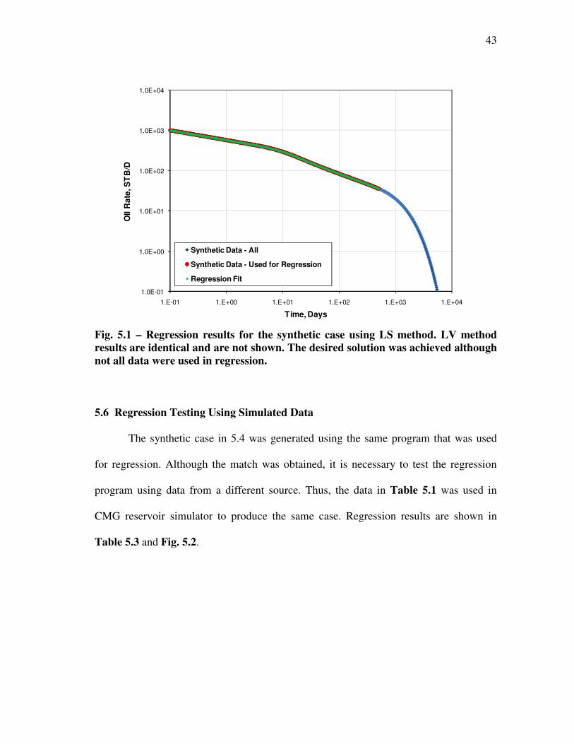
43

1.0E-01

1.0E+00

1.0E+01

1.0E+02

1.0E+03

1.0E+04

1.E-01 1.E+00 1.E+01 1.E+02 1.E+03 1.E+04

OIl R

ate

, S

TB

/D

Time, Days

Synthetic Data - All

Synthetic Data - Used for Regression

Regression Fit

Fig. 5.1 – Regression results for the synthetic case using LS method. LV method

results are identical and are not shown. The desired solution was achieved although

not all data were used in regression.

5.6 Regression Testing Using Simulated Data

The synthetic case in 5.4 was generated using the same program that was used

for regression. Although the match was obtained, it is necessary to test the regression

program using data from a different source. Thus, the data in Table 5.1 was used in

CMG reservoir simulator to produce the same case. Regression results are shown in

Table 5.3 and Fig. 5.2.

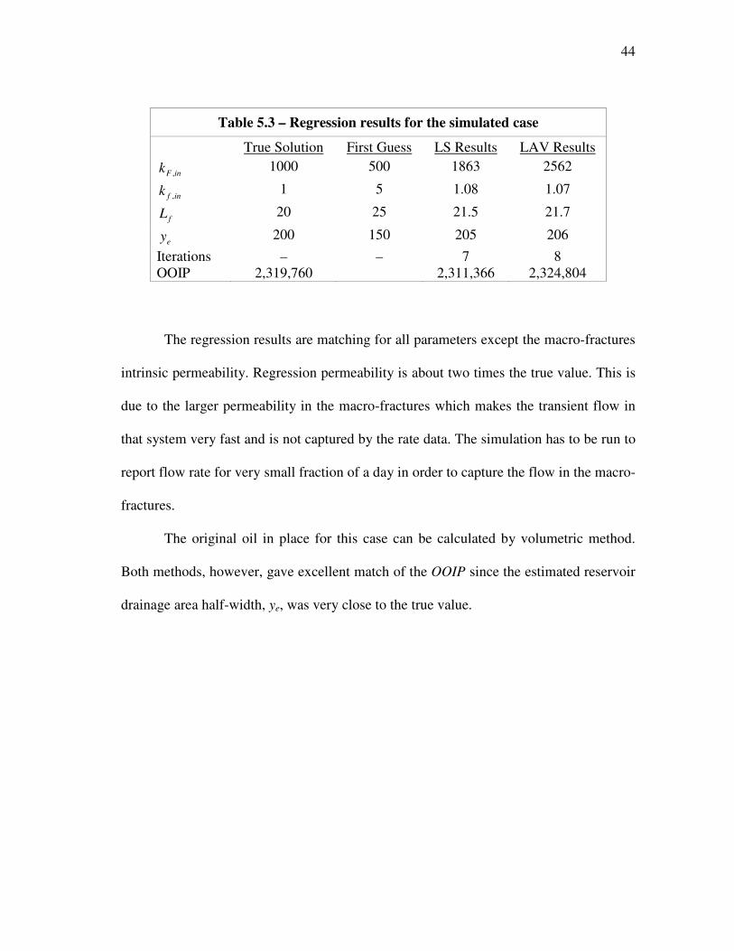
44

Table 5.3 – Regression results for the simulated case


inFk , 1000 500 1863 2562

infk , 1 5 1.08 1.07

fL 20 25 21.5 21.7

ey 200 150 205 206


OOIP 2,319,760 2,311,366 2,324,804

The regression results are matching for all parameters except the macro-fractures

intrinsic permeability. Regression permeability is about two times the true value. This is

due to the larger permeability in the macro-fractures which makes the transient flow in

that system very fast and is not captured by the rate data. The simulation has to be run to

report flow rate for very small fraction of a day in order to capture the flow in the macro-

fractures.

The original oil in place for this case can be calculated by volumetric method.

Both methods, however, gave excellent match of the OOIP since the estimated reservoir

drainage area half-width, ye, was very close to the true value.

45

1.0E-01

1.0E+00

1.0E+01

1.0E+02

1.0E+03

1.0E+04

1.E-01 1.E+00 1.E+01 1.E+02 1.E+03 1.E+04

OIl R

ate

, S

TB

/D

Time, Days

Simulation Data

Data used for regression

Regression Fit - LS

Regression Fit - LAV

Fig. 5.2 – Regression results for the simulated case using LS and LAV methods. The

match using both methods is almost identical. The solution was obtained without

including all data in regression.

5.7 Matching Noisy Data

It is known that LS regression method is affected by outliers. Thus, some noise

has been added to the synthetic data in section 5.5. The data was modified by changing

the rate by10% and -5% every 5 pints alternatively. For example, the 5th

point rate is

increased by 10% while the 10th

point rate was reduced by 5%.

The regression results are shown in Table 5.4. The LS method was affected by

the noise and the computational time increased dramatically as it took 467 iterations to

converge. The converged solution, however, is very close to the true solution.

The LAV, on the other hand, has not been affected by the noise. Thus, when

dealing with field cases, the LAV method match will be honored.

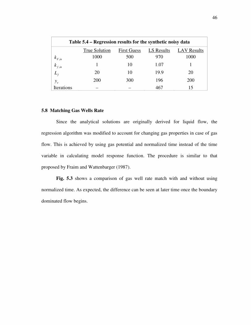
46

Table 5.4 – Regression results for the synthetic noisy data


inFk , 1000 500 970 1000

infk , 1 10 1.07 1

fL 20 10 19.9 20

ey 200 300 196 200


5.8 Matching Gas Wells Rate

Since the analytical solutions are originally derived for liquid flow, the

regression algorithm was modified to account for changing gas properties in case of gas

flow. This is achieved by using gas potential and normalized time instead of the time

variable in calculating model response function. The procedure is similar to that

proposed by Fraim and Wattenbarger (1987).

Fig. 5.3 shows a comparison of gas well rate match with and without using

normalized time. As expected, the difference can be seen at later time once the boundary

dominated flow begins.

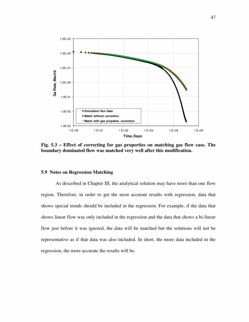
47

1.0E-03

1.0E-02

1.0E-01

1.0E+00

1.0E+01

1.0E+02

1.0E+03

1.E+00 1.E+01 1.E+02 1.E+03 1.E+04 1.E+05

Ga

Rate

, M

sc

f/d

Time, Days

Simulation Run Data

Match without correction

Match with gas propeties correction

Fig. 5.3 – Effect of correcting for gas properties on matching gas flow case. The

boundary dominated flow was matched very well after this modification.

5.9 Notes on Regression Matching

As described in Chapter III, the analytical solution may have more than one flow

region. Therefore, in order to get the most accurate results with regression, data that

shows special trends should be included in the regression. For example, if the data that

shows linear flow was only included in the regression and the data that shows a bi-linear

flow just before it was ignored, the data will be matched but the solutions will not be

representative as if that data was also included. In short, the more data included in the

regression, the more accurate the results will be.

48

CHAPTER VI

APPLICATION OF THE TRIPLE-POROSITY MODEL TO SHALE GAS

WELLS

6.1 Introduction

Shale gas reservoirs play a major role in the United State natural gas supply as

they are aggressively developed capitalizing on new technologies, namely horizontal

wells with multi-stage fracturing. It has been observed that these wells behave as though

they are controlled by transient linear flow (Bello 2009; Bello & Wattenbarger 2008,

2009, 2010; Al-Ahmadi et al. 2010). According to Medeiros et al. (2008) linear flow is

the dominant flow regime for fractured horizontal wells in tight formations for most of

their productive lives. This behavior is characterized by a negative half-slope on the log-

log plot of gas rate versus time and a straight line on the [m(pi) – m(pwf)]/qg vs. t0.5

plot

(the square-root of time plot).

Some shale gas wells, however, exhibit a bi-linear flow just before the linear

flow is observed. This behavior is characterized by a negative quarter-slope on the log-

log plot of gas rate versus time or a straight line on the [m(pi) – m(pwf)]/qg vs. t0.25

plot.

The bi-linear flow is due to two perpendicular transient linear flows occurring

simultaneously in two contiguous systems. These could be micro-fractures and matrix or

micro-fractures and macro-fractures systems.

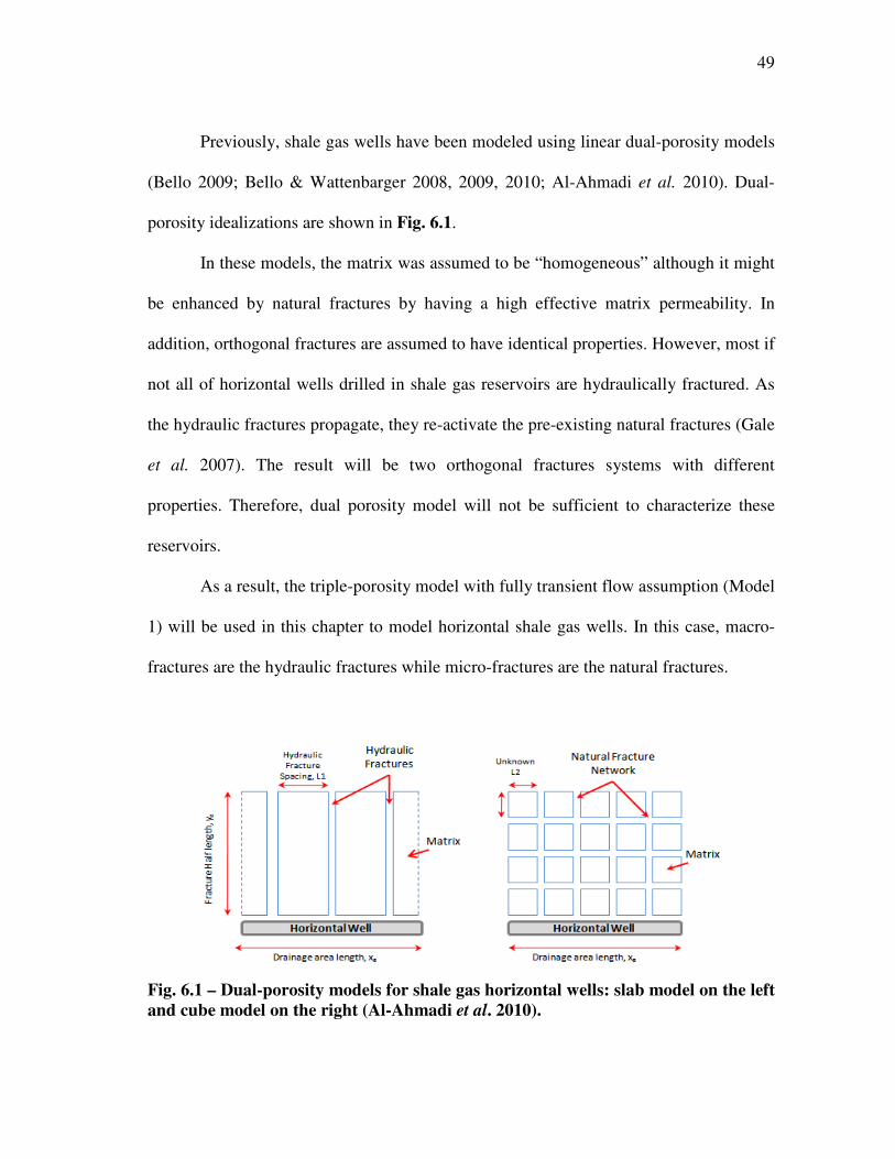
49

Previously, shale gas wells have been modeled using linear dual-porosity models

(Bello 2009; Bello & Wattenbarger 2008, 2009, 2010; Al-Ahmadi et al. 2010). Dual-

porosity idealizations are shown in Fig. 6.1.

In these models, the matrix was assumed to be “homogeneous” although it might

be enhanced by natural fractures by having a high effective matrix permeability. In

addition, orthogonal fractures are assumed to have identical properties. However, most if

not all of horizontal wells drilled in shale gas reservoirs are hydraulically fractured. As

the hydraulic fractures propagate, they re-activate the pre-existing natural fractures (Gale

et al. 2007). The result will be two orthogonal fractures systems with different

properties. Therefore, dual porosity model will not be sufficient to characterize these

reservoirs.

As a result, the triple-porosity model with fully transient flow assumption (Model

1) will be used in this chapter to model horizontal shale gas wells. In this case, macro-

fractures are the hydraulic fractures while micro-fractures are the natural fractures.

Fig. 6.1 – Dual-porosity models for shale gas horizontal wells: slab model on the left

and cube model on the right (Al-Ahmadi et al. 2010).

50

6.2 Accounting for Adsorbed Gas

Unlike tight gas reservoirs, gas in shale reservoirs is stored as compressed (free)

gas and adsorbed gas. Adsorbed gas does not usually flow until the pressure drops below

the sorption pressure. Adsorbed gas can be accounted for using Langmuir isotherm

which defines the adsorbed gas volume as

( )L

Lpp

pVV

+= ............................................................................................. (6.1)

where

V: Volume of gas currently adsorbed (scf/cuf)

VL: Langmuir’s volume (scf/cuf)

pL: Langmuir’s pressure (psia)

p: Reservoir pressure (psia)

Therefore, the analytical solutions have to account for the adsorbed gas before

applying them to shale gas wells. This can be achieved by modifying the gas

compressibility definition to include adsorbed gas. Following Bumb and McKee (1988),

the modified total compressibility is defined as

( )wwgdgft ScScccc +++=* ........................................................................... (6.2)

where dc is the desorbed gas compressibility given by

( ) ( )22pp

pVB

pp

pVc

L

LLg

Lg

LLg

dsc

+=

+=

ϕρϕ

ρ ................................................................. (6.3)

Thus, to account for adsorption, *

tc instead of tc will be used in the analytical solutions

to be applicable to shale gas wells.

51

For material balance calculations, the modified compressibility factor (z*) is used

instead of z (King 1993). z* is defined as

( )( ) scscL

scLwi

zTpp

zpTVS

zz

++−

=

ϕ1

* ..................................................................... (6.4)

Then the gas material balance equation becomes

−=

G

G

z

p

z

p p

i

i 1**

........................................................................................... (6.5)

The OGIP accounting for free and adsorbed gas can be calculated using the following

volumetric equation (Mengal 2010)

++

=

Li

iL

gi

gi

bpp

pV

B

SVG

ϕ .................................................................... (6.6)

6.3 Analysis Procedure

Due to the large number of variables involved in the triple-porosity model, non-

linear regression will be utilized to estimate a set of unknown parameters by matching

the well’s production rate. Other parameters may be assumed or estimated through other

methods. Including many variables in the regression may lead to non-uniqueness of the

converged solution.

The parameters to be found by regression are fractures intrinsic permeabilities,

drainage area half-width (hydraulic fracture half-length) and natural fractures spacing.

After the match is obtained, the well model is fully defined. Hence, the OGIP can be

calculated by volumetric method and well future production can be forecasted.

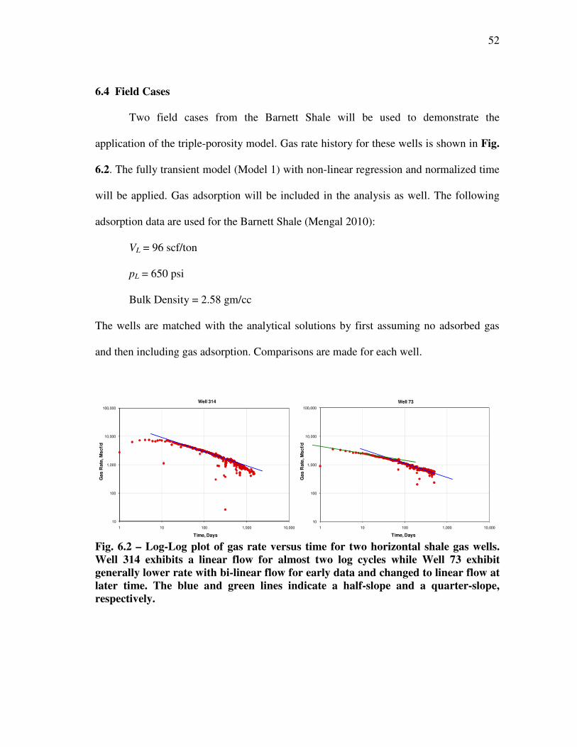
52

6.4 Field Cases

Two field cases from the Barnett Shale will be used to demonstrate the

application of the triple-porosity model. Gas rate history for these wells is shown in Fig.

6.2. The fully transient model (Model 1) with non-linear regression and normalized time

will be applied. Gas adsorption will be included in the analysis as well. The following

adsorption data are used for the Barnett Shale (Mengal 2010):

VL = 96 scf/ton

pL = 650 psi

Bulk Density = 2.58 gm/cc

The wells are matched with the analytical solutions by first assuming no adsorbed gas

and then including gas adsorption. Comparisons are made for each well.

10

100

1,000

10,000

100,000

1 10 100 1,000 10,000

Gas

Rate

, M

scf/

d

Time, Days

Well 314

10

100

1,000

10,000

100,000

1 10 100 1,000 10,000

Gas

Rate

, M

sc

f/d

Time, Days

Well 73

Fig. 6.2 – Log-Log plot of gas rate versus time for two horizontal shale gas wells.

Well 314 exhibits a linear flow for almost two log cycles while Well 73 exhibit

generally lower rate with bi-linear flow for early data and changed to linear flow at

later time. The blue and green lines indicate a half-slope and a quarter-slope,

respectively.

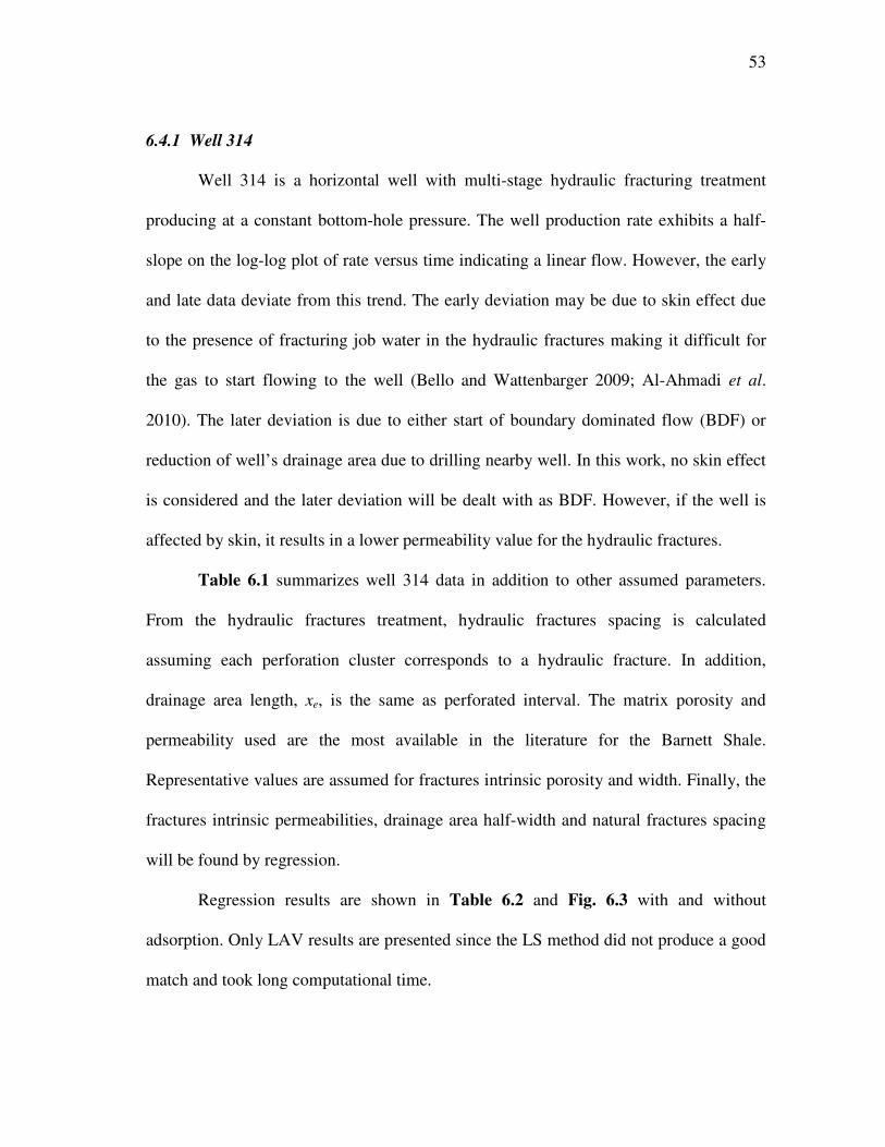
53

6.4.1 Well 314

Well 314 is a horizontal well with multi-stage hydraulic fracturing treatment

producing at a constant bottom-hole pressure. The well production rate exhibits a half-

slope on the log-log plot of rate versus time indicating a linear flow. However, the early

and late data deviate from this trend. The early deviation may be due to skin effect due

to the presence of fracturing job water in the hydraulic fractures making it difficult for

the gas to start flowing to the well (Bello and Wattenbarger 2009; Al-Ahmadi et al.

2010). The later deviation is due to either start of boundary dominated flow (BDF) or

reduction of well’s drainage area due to drilling nearby well. In this work, no skin effect

is considered and the later deviation will be dealt with as BDF. However, if the well is

affected by skin, it results in a lower permeability value for the hydraulic fractures.

Table 6.1 summarizes well 314 data in addition to other assumed parameters.

From the hydraulic fractures treatment, hydraulic fractures spacing is calculated

assuming each perforation cluster corresponds to a hydraulic fracture. In addition,

drainage area length, xe, is the same as perforated interval. The matrix porosity and

permeability used are the most available in the literature for the Barnett Shale.

Representative values are assumed for fractures intrinsic porosity and width. Finally, the

fractures intrinsic permeabilities, drainage area half-width and natural fractures spacing

will be found by regression.

Regression results are shown in Table 6.2 and Fig. 6.3 with and without

adsorption. Only LAV results are presented since the LS method did not produce a good

match and took long computational time.

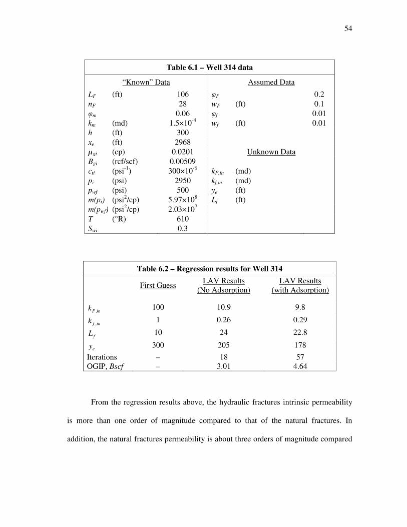
54

Table 6.1 – Well 314 data

“Known” Data Assumed Data

LF (ft) 106 φF 0.2

nF 28 wF (ft) 0.1

φm 0.06 φf 0.01

km (md) 1.5×10-4

wf (ft) 0.01

h (ft) 300

xe (ft) 2968

µgi (cp) 0.0201 Unknown Data

Bgi (rcf/scf) 0.00509

cti (psi-1

) 300×10-6

kF,in (md)

pi (psi) 2950 kf,in (md)

pwf (psi) 500 ye (ft)

m(pi) (psi2/cp) 5.97×10

8 Lf (ft)

m(pwf) (psi2/cp) 2.03×10

7

T (°R) 610

Swi 0.3

Table 6.2 – Regression results for Well 314

First Guess LAV Results

(No Adsorption)

LAV Results

(with Adsorption)

inFk , 100 10.9 9.8

infk , 1 0.26 0.29

fL 10 24 22.8

ey 300 205 178

Iterations – 18 57

OGIP, Bscf – 3.01 4.64

From the regression results above, the hydraulic fractures intrinsic permeability

is more than one order of magnitude compared to that of the natural fractures. In

addition, the natural fractures permeability is about three orders of magnitude compared

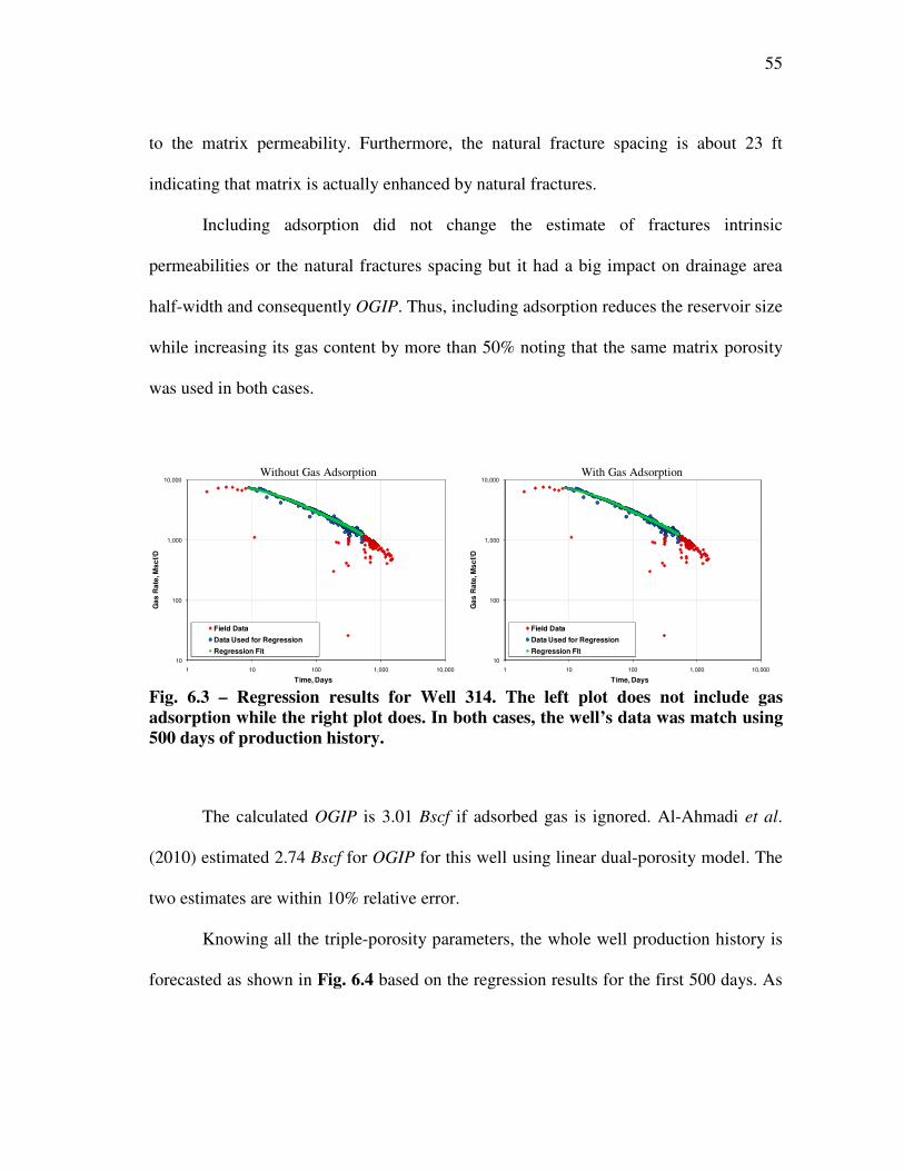
55

to the matrix permeability. Furthermore, the natural fracture spacing is about 23 ft

indicating that matrix is actually enhanced by natural fractures.

Including adsorption did not change the estimate of fractures intrinsic

permeabilities or the natural fractures spacing but it had a big impact on drainage area

half-width and consequently OGIP. Thus, including adsorption reduces the reservoir size

while increasing its gas content by more than 50% noting that the same matrix porosity

was used in both cases.

10

100

1,000

10,000

1 10 100 1,000 10,000

Ga

s R

ate

, M

sc

f/D

Time, Days

Field Data

Data Used for Regression

Regression Fit

10

100

1,000

10,000

1 10 100 1,000 10,000

Ga

s R

ate

, M

sc

f/D

Time, Days

Field Data


Regression Fit

Fig. 6.3 – Regression results for Well 314. The left plot does not include gas

adsorption while the right plot does. In both cases, the well’s data was match using

500 days of production history.

The calculated OGIP is 3.01 Bscf if adsorbed gas is ignored. Al-Ahmadi et al.

(2010) estimated 2.74 Bscf for OGIP for this well using linear dual-porosity model. The

two estimates are within 10% relative error.

Knowing all the triple-porosity parameters, the whole well production history is

forecasted as shown in Fig. 6.4 based on the regression results for the first 500 days. As

Without Gas Adsorption With Gas Adsorption

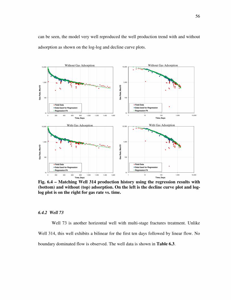
56

can be seen, the model very well reproduced the well production trend with and without

adsorption as shown on the log-log and decline curve plots.

10

100

1,000

10,000

0 200 400 600 800 1,000 1,200 1,400 1,600

Ga

s R

ate

, M

scf/

D

Time, Days

Field Data


Regression Fit

10

100

1,000

10,000

1 10 100 1,000 10,000

Ga

s R

ate

, M

sc

f/D

Time, Days

Field Data


Regression Fit

10

100

1,000

10,000

0 200 400 600 800 1,000 1,200 1,400 1,600

Ga

s R

ate

, M

scf/

D

Time, Days

Field Data


Regression Fit10

100

1,000

10,000

1 10 100 1,000 10,000

Ga

s R

ate

, M

sc

f/D

Time, Days

Field Data


Regression Fit

Fig. 6.4 – Matching Well 314 production history using the regression results with

(bottom) and without (top) adsorption. On the left is the decline curve plot and log-

log plot is on the right for gas rate vs. time.

6.4.2 Well 73

Well 73 is another horizontal well with multi-stage fractures treatment. Unlike

Well 314, this well exhibits a bilinear for the first ten days followed by linear flow. No

boundary dominated flow is observed. The well data is shown in Table 6.3.

With Gas Adsorption With Gas Adsorption

Without Gas Adsorption Without Gas Adsorption

57

All rate data were used for regression since no good match was obtained using

fewer data points. The regression results are shown in Table 6.4 and Fig. 6.5. As the

case with Well 314, LAV regression method was used. As can be seen in Fig. 6.5, the

regression match described the well trend perfectly with and without gas adsorption.

Table 6.3 – Well 73 data

“Known” Data Assumed Data

LF (ft) 79 φF 0.2

nF 18 wF (ft) 0.1

φm 0.06 φf 0.01

km (md) 1.5×10-4

wf (ft) 0.01

h (ft) 300

xe (ft) 1420

µgi (cp) 0.0201 Unknown Data

Bgi (rcf/scf) 0.00509

cti (psi-1

) 300×10-6

kF,in (md)

pi (psi) 2950 kf,in (md)

pwf (psi) 500 ye (ft)

m(pi) (psi2/cp) 5.97×10

8 Lf (ft)

m(pwf) (psi2/cp) 2.03×10

7

T (°R) 610

Swi 0.3

Table 6.4 – Regression results for Well 73

First Guess LAV Results

(No Adsorption)

LAV Results

(with Adsorption)

inFk , 10 3.7 3.3

infk , 0.5 0.1 0.11

fL 15 23 22

ey 250 185 163

Iterations – 13 13

OGIP, Bscf – 1.32 2.05

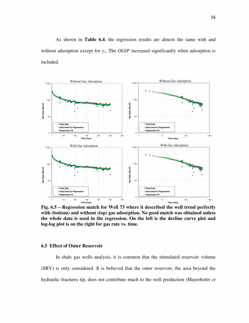
58

As shown in Table 6.4, the regression results are almost the same with and

without adsorption except for ye. The OGIP increased significantly when adsorption is

included.

10

100

1,000

10,000

0 100 200 300 400 500 600

Ga

s R

ate

, M

sc

f/D

Time, Days

Field Data


Regression Fit

10

100

1,000

10,000

1 10 100 1,000

Ga

s R

ate

, M

sc

f/D

Time, Days

Field Data


Regression Fit

10

100

1,000

10,000

0 100 200 300 400 500 600

Ga

s R

ate

, M

sc

f/D

Time, Days

Field Data


Regression Fit

10

100

1,000

10,000

1 10 100 1,000

Ga

s R

ate

, M

sc

f/D

Time, Days

Field Data


Regression Fit

Fig. 6.5 – Regression match for Well 73 where it described the well trend perfectly

with (bottom) and without (top) gas adsorption. No good match was obtained unless

the whole data is used in the regression. On the left is the decline curve plot and

log-log plot is on the right for gas rate vs. time.

6.5 Effect of Outer Reservoir

In shale gas wells analysis, it is common that the stimulated reservoir volume

(SRV) is only considered. It is believed that the outer reservoir, the area beyond the

hydraulic fractures tip, does not contribute much to the well production (Mayerhofer et

Without Gas Adsorption Without Gas Adsorption

With Gas Adsorption With Gas Adsorption

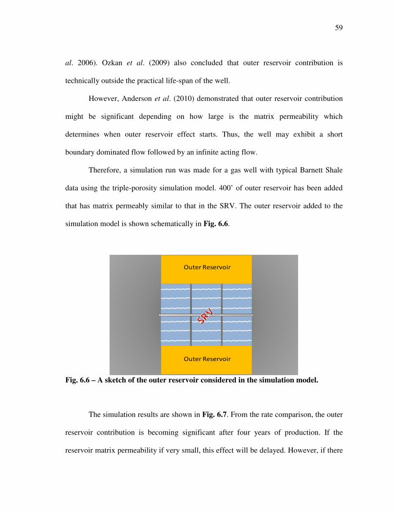
59

al. 2006). Ozkan et al. (2009) also concluded that outer reservoir contribution is

technically outside the practical life-span of the well.

However, Anderson et al. (2010) demonstrated that outer reservoir contribution

might be significant depending on how large is the matrix permeability which

determines when outer reservoir effect starts. Thus, the well may exhibit a short

boundary dominated flow followed by an infinite acting flow.

Therefore, a simulation run was made for a gas well with typical Barnett Shale

data using the triple-porosity simulation model. 400’ of outer reservoir has been added

that has matrix permeably similar to that in the SRV. The outer reservoir added to the

simulation model is shown schematically in Fig. 6.6.

Outer Reservoir

Outer Reservoir

Fig. 6.6 – A sketch of the outer reservoir considered in the simulation model.

The simulation results are shown in Fig. 6.7. From the rate comparison, the outer

reservoir contribution is becoming significant after four years of production. If the

reservoir matrix permeability if very small, this effect will be delayed. However, if there

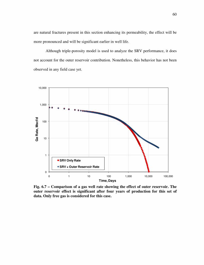
60

are natural fractures present in this section enhancing its permeability, the effect will be

more pronounced and will be significant earlier in well life.

Although triple-porosity model is used to analyze the SRV performance, it does

not account for the outer reservoir contribution. Nonetheless, this behavior has not been

observed in any field case yet.

0

1

10

100

1,000

10,000

0 1 10 100 1,000 10,000 100,000

Ga

Ra

te, M

sc

f/d

Time, Days

SRV Only Rate

SRV + Outer Reservoir Rate

Fig. 6.7 – Comparison of a gas well rate showing the effect of outer reservoir. The

outer reservoir effect is significant after four years of production for this set of

data. Only free gas is considered for this case.

61

6.6 Chapter Summary

Triple-porosity Model 1 was applied to shale gas wells. Gas adsorption was

incorporated in the model. The model successfully matched well production rate using

the non-linear regression with and without gas adsorption. When adsorbed gas is

included, it resulted in a smaller reservoir size but the OGIP is increased noticeably.

62

CHAPTER VII

CONCLUSIONS AND RECOMMENDATIONS

7.1 Conclusions

The major conclusions from this work can be summarized as follows:

1. New triple-porosity (dual-fracture) solutions have been developed for

fractured linear reservoirs.

2. Six flow regions can be identified for fully transient triple-porosity model

(Model 1)

3. The new model has been verified by reducing it to simpler models such as

dual and single (homogeneous) porosity models and by comparing it to

reservoir simulation.

4. The newly derived fracture functions are applicable to radial flow.

5. The derived solutions are also applicable to gas flow using gas potential and

normalized time.

6. Least absolute value regression method proves to be robust in matching

noisy data and can be used effectively with triple-porosity model to match

field data.

7. Triple-porosity fully transient model (Model 1) is applicable to fractured

shale gas horizontal wells when gas adsorption is incorporated. The model

can be used to match field data, characterize well drainage area, determine

reservoir size and OGIP and forecast future production.

63

7.2 Recommendations

The followings can be recommended to add to the usefulness of this work:

1. The triple-porosity model was derived for sequential flow. Thus, other flow

combinations such as simultaneous flow may worth investigation.

2. Including skin factor in the regression variables.

3. Development of analysis equation for each flow region and use that for

analyzing well performance. More properties will be estimated from each

region than using regression to match the whole well history.

4. Using derivative analysis to identify each flow region accurately.

5. Using superposition with respect to time to model variable rate and variable

bottom-hole pressure cases.

64

NOMENCLATURE

Acw cross-sectional area to flow defined as 2hxe, ft2

Acm total matrix surface area draining into fracture system, ft2

Bgi formation volume factor at initial reservoir pressure, rcf/scf

ct total compressibility, psi-1

E objective function

gr

objective function gradient

h reservoir thickness, ft

H Hessian matrix

kF macro-fractures bulk permeability, md

kf micro-fracture bulk permeability, md

kF,in macro-fracture intrinsic permeability, md

kf,in micro-fracture intrinsic permeability, md

km matrix permeability, md

LF macro-fractures spacing, ft

Lf micro-fractures spacing, ft

m(p) pseudopressure (gas), psi2/cp

pD dimensionless pressure (transient triple porosity model)

pi initial reservoir pressure, psi

pwf wellbore flowing pressure, psi

qD dimensionless rate (transient triple porosity model)

65

qDL dimensionless rate based on Acw0.5

and kF (rectangular geometry, triple

porosity)

qg gas rate, Mscf/day

rw wellbore radius, ft

Sgi initial gas saturation, fraction

Swi initial water saturation, fraction

T absolute temperature, oR

t time, days

tDAcw dimensionless time based on Acw and kF (rectangular geometry, triple-

porosity)

tesr time to end of straight line on the square root of time plot, days

Vb total system bulk volume, ft3

V bulk volume fraction, dimensionless

xe drainage area length (rectangular geometry), ft

yDe dimensionless reservoir half-width (rectangular geometry)

ye drainage area half-width (rectangular geometry), equivalent to fracture

half-length, ft

Greek symbols

α Warren & Root shape factor

αr

vector of unknown regression parameters

λ dimensionless interporosity parameter

66

µ viscosity, cp

ω dimensionless storativity ratio

φ porosity

Subscripts

i initial

F macro-fracture (hydraulic fracture)

f micro-fracture (natural fracture)

m matrix

t =F+f+m total system (macro-fracture +micro-fracture + matrix)

Superscripts

x Laplace transform of variable x

xk k

th iteration of variable x

Txr

transpose of vector xr

67

REFERENCES

Abdassah, D. and Ershaghi, I. 1986. Triple-Porosity Systems for Representing Naturally

Fractured Reservoirs. SPE Form Eval (April): 113 – 127. SPE-13409-PA.

Al-Ahmadi, H. A., Almarzooq, A. M. and Wattenbarger, R. A. 2010. Application of

Linear Flow Analysis to Shale Gas Wells – Field Cases. Paper SPE 130370

presented at the 2010 Unconventional Gas Conference, Pittsburgh, Pennsylvania,

23 – 25 February.

Al-Ghamdi, A. and Ershaghi, I. 1996. Pressure Transient Analysis of Dually Fractured

Reservoirs. SPE J. (March): 93 – 100. SPE-26959-PA.

Al-Hussainy, R., Ramey, H. J., Jr., and Crawford, P. B. 1966. The Flow of Real Gas

Through Porous Media. J. Pet Tech (May): 624 – 636. SPE-1243A-PA

Anderson, D. M., Nobakht, M., Moghadam, S. and Mattar, L. 2010. Analysis of

Production Data from Fractured Shale Gas Wells. Paper SPE 131787 presented at

the SPE Unconventional Gas Conference, Pittsburgh, Pennsylvania, 23 – 25

February.

Barenblatt, G. I., Zhelto, I. P. and Kochina, I. N. 1960. Basic Concepts of the Theory of

Seepage of Homogeneous Liquids in Fissured Rocks. Journal of Applied

Mathematical Mechanics (USSR) 24 (5): 852 – 864.

Barrodale, I. and Roberts, F. D. K. 1974. Solution of an Overdetermined System of

Equations in the l1 Norm. Communication of the ACM 17 (6): 319 – 320.

Bello, R.O. 2009. Rate Transient Analysis in Shale Gas Reservoirs with Transient Linear

Behavior. Ph.D. Dissertation, Texas A&M U., College Station, Texas.

Bello, R. O. and Wattenbarger, R. A. 2008. Rate Transient Analysis in Naturally

Fractured Shale Gas Reservoirs. Paper SPE 114591 presented at the CIPC/SPE

Gas Technology Symposium 2008 Joint Conference, Calgary, Alberta, Canada,

16 – 19 June.

Bello, R. O. and Wattenbarger, R. A. 2009. Modeling and Analysis of Shale Gas

Production with a Skin Effect. Paper CIPC 2009-082 presented at the Canadian

International Petroleum Conference, Calgary, Alberta, Canada, 16 – 18 June.

68

Bello, R. O. and Wattenbarger, R. A. 2010. Multi-stage Hydraulically Fractured Shale

Gas Rate Transient Analysis. Paper SPE 126754 presented at the SPE North

Africa Technical Conference and Exhibition held in Cairo, Egypt, 14 – 17

February.

Brown, M., Ozkan, E., Raghavan, R. and Kazemi, H. 2009. Practical Solutions for

Pressure Transient Responses of Fractured Horizontal Wells in Unconventional

Reservoirs. Paper SPE 125043 presented at the Annual Technical Conference and

Exhibition, New Orleans, Louisiana, 4 – 7 October.

Bumb, A. C and McKee, C. R. 1988. Gas-Well Testing in the Pressure of Desorption for

Coalbed Methane and Devonian Shale. SPE Form Eval (March): 179 - 185. SPE-

15227-PA.

Cheney, E.W. and Kincaid, R. D. 1985. Numerical Mathematics and Computing, 2nd

edition. Monterey, California: Brooks/Cole Publishing Company.

de Swaan, O. A. 1976. Analytic Solutions for Determining Naturally Fractured

Reservoir Properties by Well Testing. SPE J. (June): 117 – 122. SPE-5346-PA.

Dreier, J. 2004. Pressure-Transient Analysis of Wells in Reservoirs with a Multiple

Fracture Network. M.Sc. Thesis, Colorado School of Mines, Golden, Colorado.

Dreier, J., Ozkan, E. and Kazemi, H. 2004. New Analytical Pressure-Transient Models

to Detect and Characterize Reservoirs with Multiple Fracture Systems. Paper SPE

92039 presented at the SPE International Petroleum Conference in Mexico,

Puebla, Mexico, 8 – 9 November.

El-Banbi, A.H. 1998. Analysis of Tight Gas Wells. Ph.D. Dissertation, Texas A &M U.,

College Station, Texas.

Fraim, M. L. and Wattenbarger, R. A. 1987. Gas Reservoir Decline-Curve Analysis

Using Type Curve with Real Gas Pseudopressure and Normalized Time. SPE

Form Eval (December): 671 – 682. SPE-14238-PA.

Gale, J. F., Reed, R. M. and Holder, J. 2007. Natural Fractures in the Barnett Shale and

Their Importance for Hydraulic Fracture Treatments. AAPG Bulletin. 91 (4): 603

– 622.

Jalali, Y. and Ershaghi, I. 1987. Pressure Transient Analysis of Heterogeneous Naturally

Fractured Reservoirs. Paper SPE 16341 presented at the SPE California Regional

Meeting, Ventura, California, 8 – 10 April.

Kazemi, H. 1969. Pressure Transient of Naturally Fractured Reservoirs with Uniform

Fracture Distribution. SPE J. (December):451– 462. SPE-2156A-PA.

69

King, G. R. 1993. Material-Balance Techniques for Coal-Seam and Devonian Shale Gas

Reservoirs with Limited Water Influx. SPE Res Eng (February): 67 – 72. SPE-

20730-PA.

Liu, C. Q. 1981. Exact Solution for the Compressible Flow Equations through a Medium

with Triple-Porosity. Applied Mathematics and Mechanics 2 (4): 457 – 462.

Liu, C. Q. 1983. Exact Solution of Unsteady Axisymmetrical Two-Dimensional Flow

through Triple Porous Media. Applied Mathematics and Mechanics 4 (5): 717 –

724.

Liu, J. C., Bodvarsson, G. S. and Wu, Y. S. 2003. Analysis of Flow Behavior in

Fractured Lithophysal Reservoirs. Journal of Contaminant Hydrology 62-63: 189

– 211.

Mayerhofer, M. J., Lolon, E. P., Youngblood, J. E. and Heinze, J. R. 2006. Integration of

Microseismic Fracture Mapping Results with Numerical Fracture Network

Production Modeling in the Barnett Shale. Paper SPE 102103 presented at the

Annual Technical Conference and Exhibition, San Antonio, Texas, 24 – 27

September.

Medeiros, F., Ozkan, E. and Kazemi, H. 2008. Productivity and Drainage Area of

Fractured Horizontal Wells in Tight Gas Reservoirs. SPE Res Eval & Eng

(October): 902 – 911. SPE-108110-PA.

Mengal, S. A. 2010. Accounting for Adsorbed Gas and Its Effect on Production

Behavior of Shale Gas Reservoirs. M.Sc. Thesis, Texas A&M U., College Station,

Texas.

Nelson, R. A. 2001. Geologic Analysis of Naturally Fractured Reservoirs, 2nd

edition.

Woburn, Massachusetts: Butterworth-Heinemann.

Ozkan, E., Brown, M., Raghavan, R. and Kazemi, H. 2009. Comparison of Fractured

Horizontal-Well Performance in Conventional and Unconventional Reservoirs.

Paper SPE 121290 presented at the SPE Western Regional Meeting, San Jose,

California, 24 – 26 March.

Ozkan, E., Ohaeri, U. and Raghavan, R. 1987. Unsteady Flow to a Well Produced at a

Constant Pressure in Fractured Reservoir. SPE Form Eval (June): 186 - 200. SPE-

9902-PA.

Rosa, A. J. and Horne, R. N. 1995. Automated Well Test Analysis Using Robust (LAV)

Nonlinear Parameter Estimation. SPE Advanced Technology Series 3 (1): 95 –

102. SPE-22679-PA.

70

Rosa, A. J. and Horne, R. N. 1996. New Approaches for Robust Nonlinear Parameter

Estimation in Automated Well Test Analysis Using the Least Absolute Value

Criterion. SPE Advanced Technology Series 4 (1): 21 – 27. SPE-26964-PA.

Sarma, P. and Aziz, K. 2006. New Transfer Functions for Simulation of Naturally

Fractured Reservoirs with Dual-Porosity Models. SPE J. (September): 328 – 340.

SPE-90231-PA.

Stehfest, H. 1970. Algorithm 358 – Numerical Inversion of Laplace Transforms.

Communication of the ACM 13 (1): 47 – 49.

Van Everdingen, A. F. and Hurst, W. 1949. The Application of the Laplace

Transformation to Flow Problems in Reservoirs. Trans., AIME, 186: 305 – 324.

Warren, J. E. and Root, P. J. 1963. The Behavior of Naturally Fractured Reservoirs.

SPE J. (September): 245 – 255. SPE-426-PA.

Wattenbarger, R.A. 2007. Some Reservoir Performance Aspects of Unconventional Gas

Production. Private Conference Presentation, Lake Louise, Alberta, Canada.

Wu, Y. S., Liu, H. H. and Bodvarsson, G. S. 2004. A Triple-Continuum Approach for

Modeling Flow and Transport Processes in Fractured Rock. Journal of

Contaminant Hydrology 73: 145 – 179.

71

APPENDIX A

LINEAR FLOW SOLUTIONS FOR FRACTURED LINEAR RESERVOIRS

Laplace transformation with respect to dimensionless time, tDAc, is used to derive

the rate solutions in fractured reservoirs. This transformation enables us to reduce the

second-order partial differential flow equation to a second-order ordinary differential

equation in Laplace domain. The solution is then easy to obtain in Laplace domain

which can be inverted to time domain using Stehfest algorithm (Stehfest 1970).

Upon transformation, the differential equation in Laplace domain that describes

the main flow in linear reservoir system shown in Fig. A-1 is given by

( ) 02

2

=−∂

∂DLF

D

DLF psfsy

p .............................................................................. (A-1)

This form of equation makes it easy to solve for different fractured reservoirs

with varying degree of complexity by having different fracture function, ( )sf . For the

simplest case, i.e., homogeneous reservoir, ( ) 1=sf . s in Eq. A-1 is the Laplace

transform parameter.

Linear flow solutions for fractured linear reservoirs assuming dual-porosity

system was first developed by El-Banbi (1998).

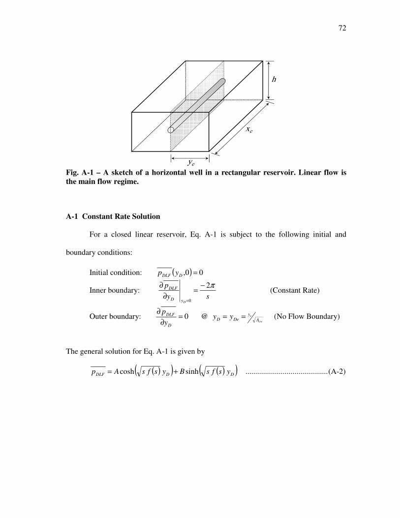
72

h

xe

ye Fig. A-1 – A sketch of a horizontal well in a rectangular reservoir. Linear flow is

the main flow regime.

A-1 Constant Rate Solution

For a closed linear reservoir, Eq. A-1 is subject to the following initial and

boundary conditions:


Inner boundary: sy

p

DyD

DLF π2

0

−=

∂

∂

=

(Constant Rate)

Outer boundary: cw

e

A

yDeD

D

DLF yyy

p===

∂

∂@0 (No Flow Boundary)

The general solution for Eq. A-1 is given by

( )( ) ( )( )DDDLF ysfsBysfsAp sinhcosh += .......................................... (A-2)

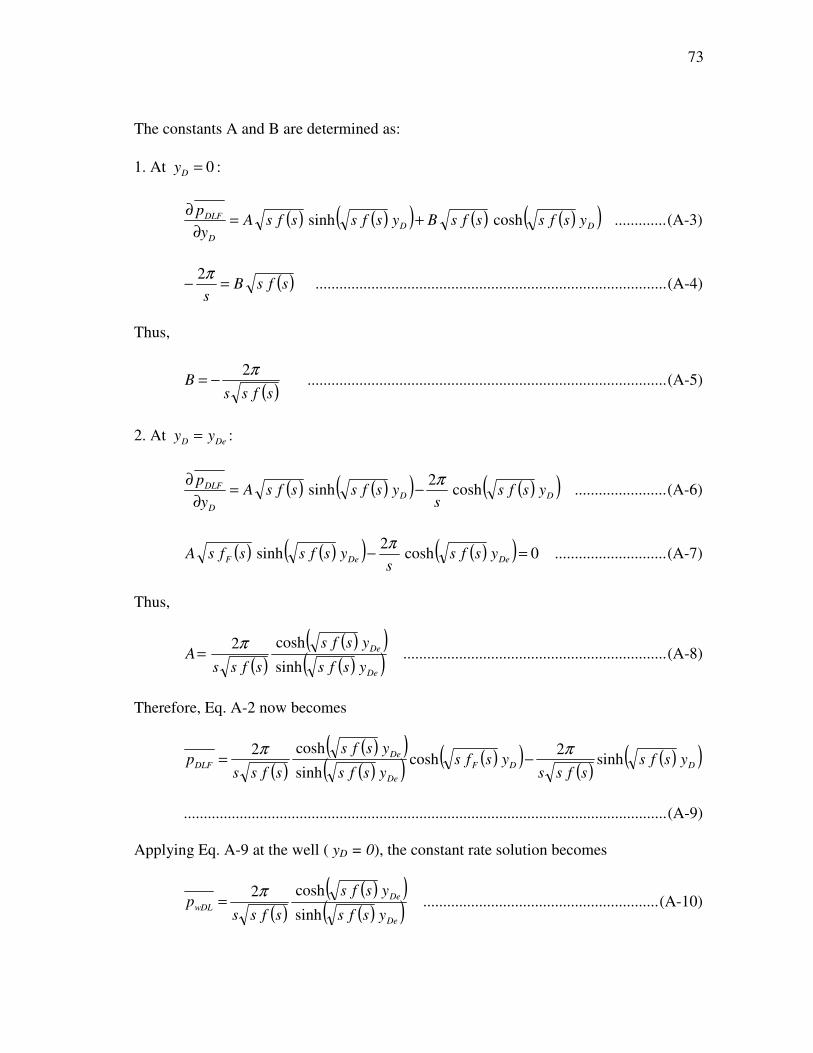
73

The constants A and B are determined as:

1. At 0=Dy :

( ) ( )( ) ( ) ( )( )DD

D

DLF ysfssfsBysfssfsAy

pcoshsinh +=

∂

∂ ............. (A-3)

( )sfsBs

=−π2

........................................................................................ (A-4)

Thus,

( )sfssB

π2−= .......................................................................................... (A-5)

2. At DeD yy = :

( ) ( )( ) ( )( )DD

D

DLF ysfss

ysfssfsAy

pcosh

2sinh

π−=

∂

∂ ....................... (A-6)

( ) ( )( ) ( )( ) 0cosh2

sinh =− DeDeF ysfss

ysfssfsAπ

............................ (A-7)

Thus,

( )( )( )( )( )De

De

ysfs

ysfs

sfssA

sinh

cosh2π= .................................................................. (A-8)

Therefore, Eq. A-2 now becomes

( )( )( )( )( ) ( )( )

( )( )( )DDF

De

De

DLF ysfssfss

ysfsysfs

ysfs

sfssp sinh

2cosh

sinh

cosh2 ππ−=

......................................................................................................................... (A-9)

Applying Eq. A-9 at the well ( yD = 0), the constant rate solution becomes

( )( )( )( )( )De

De

wDLysfs

ysfs

sfssp

sinh

cosh2π= ........................................................... (A-10)

74

Upon Algebraic manipulations of Eq. A-10 (El-Banbi 1998; Bello 2009)

( )( )( )( )( )

−−

−+=

De

De

wDLysfs

ysfs

sfssp

2exp1

2exp12π ................................................. (A-11)

A-2 Constant Pressure Solution

In Laplace domain, the constant rate and constant pressure solutions at the

wellbore are related by Eq. A-12 (Van Everdingen and Hurst 1949)

2

1

sqp DLwDL =× .......................................................................................... (A-12)

Therefore, the solution for constant pressure case (El-Banbi 1998) is

( )( )( )( )( )

−−

−+=

De

De

DL ysfs

ysfs

sfs

s

q 2exp1

2exp121 π .................................................... (A-13)

In subsequent appendixes, different fracture functions, ( )sf , are derived. The above

solutions are then used to get the final solution.

A-3 Accounting for Wellbore Storage and Skin

Once the fracture function, ( )sf , is derived for the case without skin and

wellbore storage effects, El-Banbi’s solutions that account for these effects can be used.

These solutions are already programmed in the Stehfest VBA program. Refer to El-

Banbi Dissertation (El-Banbi 1998) for complete list of solutions.

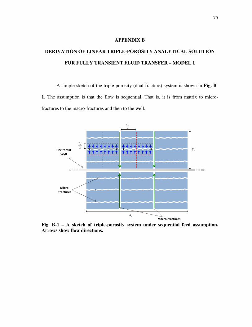
75

APPENDIX B

DERIVATION OF LINEAR TRIPLE-POROSITY ANALYTICAL SOLUTION

FOR FULLY TRANSIENT FLUID TRANSFER – MODEL 1

A simple sketch of the triple-porosity (dual-fracture) system is shown in Fig. B-

1. The assumption is that the flow is sequential. That is, it is from matrix to micro-

fractures to the macro-fractures and then to the well.

2

fL

ex

ey

Micro-

fractures

Macro-fractures

Horizontal

Well

2

FL

Fig. B-1 – A sketch of triple-porosity system under sequential feed assumption.

Arrows show flow directions.

76

B-1 Matrix Equation

Since the flow transfer from matrix to fractures is under transient condition, the

matrix equation is given by:

( )t

pVc

z

pk m

mtmm

∂

∂=

∂

∂ϕ

µ 2

2

............................................................................... (B-1)

Or

[ ]t

p

k

cV

z

p m

m

mtm

∂

∂=

∂

∂ µϕ2

2

................................................................................. (B-2)

Note: z here is a direction parallel to y-axis. It is not the vertical direction.

B-2 Micro-fracture Equation

( )t

pVcq

x

pk f

ftmsource

ff

∂

∂=+

∂

∂ϕ

µ,2

2

................................................................ (B-3)

msourceq , is a source term of flow from matrix to the micro-fracture under transient flow

and can be written as

22

,

1

fLf

z

mm

Lmsourcez

pkq

=∂

∂−=

µ ............................................................................ (B-4)

Thus, the final form of micro-fractures equation is

( )2

2

2

21

fLf

z

mm

L

f

ft

ff

z

pk

t

pVc

x

pk

=∂

∂+

∂

∂=

∂

∂

µϕ

µ .................................................. (B-5)

[ ]

22

2

21

fLf

z

m

f

m

L

f

f

ftf

z

p

k

k

t

p

k

cV

x

p

=∂

∂+

∂

∂=

∂

∂ µϕ .................................................... (B-6)

77

B-3 Macro-fracture Equation

The macro-fractures receives flow from the micro-fractures and the flow can be

modeled using the equation

( )t

pVcq

y

pk F

FtfsourceFF

∂

∂=+

∂

∂ϕ

µ,2

2

................................................................ (B-7)

fsourceq , is the source term of flow from micro-fractures to the macro-fracture under

transient flow and can be written as

22

,

1

FLF

x

ff

Lfsourcex

pkq

=∂

∂−=

µ ............................................................................. (B-8)

Thus, the final form of micro-fractures equation is

( )2

22

2 1

FLF

x

ff

L

F

FtFF

x

pk

t

pVc

y

pk

=∂

∂+

∂

∂=

∂

∂

µϕ

µ .................................................. (B-9)

[ ]

22

2

21

FLF

x

f

F

f

L

F

F

FtF

x

p

k

k

t

p

k

cV

y

p

=∂

∂+

∂

∂=

∂

∂ µϕ .................................................. (B-10)

B-4 System of Equations with Initial and Boundary Conditions

Matrix: [ ]

t

p

k

cV

z

p m

m

mtm

∂

∂=

∂

∂ µϕ2

2

........................................................... (B-2)

Micro-fractures: [ ]

22

2

21

fLf

z

m

f

m

L

f

f

ftf

z

p

k

k

t

p

k

cV

x

p

=∂

∂+

∂

∂=

∂

∂ µϕ ............................. (B-6)

Macro-fractures: [ ]

22

2

21

FLF

x

f

F

f

L

F

F

FtF

x

p

k

k

t

p

k

cV

y

p

=∂

∂+

∂

∂=

∂

∂ µϕ ............................ (B-10)

78

Initial and boundary conditions are:

Matrix:

Initial condition: ( ) im pzp =0,


∂z

z

pm

Outer boundary: 2

@f

fm

Lzpp ==

Micro-fractures:

Initial condition: ( )if pxp =0,


∂x

x

p f

Outer boundary: 2

@ FFf

Lxpp ==

Macro-fractures:

Initial condition: ( ) iF pyp =0,

Inner boundary: 0=

∂

∂−=

y

FcwF

y

pAkq

µ

Outer boundary: eF yyy

p==

∂

∂@0

B-5 System Dimensionless Equations with Initial and Boundary Conditions

Matrix: DAc

DLm

fmAc

m

D

DLm

t

p

z

p

∂

∂=

∂

∂

,

2

2 3

λ

ω ......................................................... (B-11)

Micro-fractures:

1,

,

,

2

2 3

=∂

∂+

∂

∂=

∂

∂

DzD

DLm

FfAc

fmAc

DAc

DLf

FfAc

f

D

DLf

z

p

t

p

x

p

λ

λ

λ

ω ................................ (B-12)

Macro-fractures:

1

,

2

2

3=

∂

∂+

∂

∂=

∂

∂

DxD

DLfFfAc

DAc

DLFF

D

DLF

x

p

t

p

y

p λω ................................ (B-13)

79

Dimensionless initial and boundary conditions are:

Matrix:



∂D

D

DLm zz

p


Micro-fractures:



∂D

D

DLfx

x

p


Macro-fractures:


Inner boundary: π2

0

−=∂

∂

=DyD

DLF

y

p

Outer boundary: cw

e

A

y

DeD

D

DLF yyy

p===

∂

∂@0

B-6 Laplace Transformation

In order to solve the above system of differential equations, they have to be transformed

into Laplace domain for easier solving as detailed below.

Matrix equation:

∂

∂=

∂

∂

DAc

DLm

fmAc

m

D

DLm

t

p

z

p

,

2

2 3

λ

ωLL .................................................................. (B-14)

( )[ ]0,3

,

2

2

DDLmDLm

fmAc

m

D

DLm zppsz

p−=

∂

∂

λ

ω ......................................................... (B-15)

80

The initial and boundary conditions in Laplace domain are:



∂D

D

DLm zz

p


Using the initial condition, Eq. B-15 becomes

[ ]03

,

2

2

−=∂

∂DLm

fmAc

m

D

DLm psz

p

λ

ω ........................................................................ (B-16)

03

,

2

2

=−∂

∂DLm

fmAc

m

D

DLm psz

p

λ

ω .......................................................................... (B-17)

The general solution for Eq. B-17 is given by

+

= D

fmAc

mD

fmAc

mDLm z

sBz

sAp

,,

3sinh

3cosh

λ

ω

λ

ω ...................................... (B-18)


1. 0=Dz :

B = 0 ........................................................................................................... (B-19)

2. 1=Dz :

=

fmAc

m

DLf

s

pA

,

3cosh

λ

ω ................................................................................... (B-20)

81

Therefore, the final solution for Eq. B-17 is

= D

fmAc

m

fmAc

m

DLf

DLm zs

s

pp

,

,

3cosh

3cosh

λ

ω

λ

ω ................................................. (B-21)

Micro-fractures equation:

∂

∂+

∂

∂=

∂

∂

=1,

,

,

2

2 3

DzD

DLm

FfAc

fmAc

DAc

DLf

FfAc

f

D

DLf

z

p

t

p

x

p

λ

λ

λ

ωLL ........................................ (B-22)

( )[ ]1,

,

,

2

2

0,3

=∂

∂+−=

∂

∂

DzD

DLm

FfAc

fmAc

DDLfDLf

FfAc

f

D

DLf

z

pxpps

x

p

λ

λ

λ

ω ............................... (B-23)




∂D

D

DLfx

x

p



1,

,

,

2

2 3

=∂

∂+=

∂

∂

DzD

DLm

FfAc

fmAc

DLf

FfAc

f

D

DLf

z

pps

x

p

λ

λ

λ

ω ..................................................... (B-24)

Now, differentiating Eq. B-21, we have

=

∂

∂

= fmAc

m

fmAc

mDLf

zD

DLm ssp

z

p

D,,1

3tanh

3

λ

ω

λ

ω ................................................... (B-25)

82

Substituting Eq. B-25 in B-24

+=

∂

∂

fmAc

m

fmAc

m

FfAc

fmAc

FfAc

f

DLf

D

DLf ss

sps

x

p

,,,

,

,

2

23

tanh33

λ

ω

λ

ω

λ

λ

λ

ω ........................... (B-26)

Or in short form

( ) 02

2

=−∂

∂DLff

D

DLfpsfs

x

p ............................................................................ (B-27)

where ( )sf f is

( )

+=

fmAc

m

fmAc

m

FfAc

fmAc

FfAc

f

f

ss

ssf

,,,

,

,

3tanh

33

λ

ω

λ

ω

λ

λ

λ

ω .......................................... (B-28)

The general solution for Eq. B-28 is given by

( )( ) ( )( )DfDfDLf xsfsBxsfsAp sinhcosh += ....................................... (B-29)


1. 0=Dx :

B = 0 ........................................................................................................... (B-30)

2. 1=Dx :

( )( )sfs

pA

f

DLF

cosh= .................................................................................... (B-31)

Therefore, the final solution for Eq. B-28 is

( )( ) ( )( )Df

f

DLFDLf xsfs

sfs

pp cosh

cosh= ................................................... (B-32)

83

Macro-fractures equation:

∂

∂+

∂

∂=

∂

∂

=1

,

2

2

3DxD

DLfFfAc

DAc

DLFF

D

DLF

x

p

t

p

y

p λωLL ............................................ (B-33)

( )[ ]1

,

2

2

30,

=∂

∂+−=

∂

∂

DxD

DLfFfAc

DDLFDLFF

D

DLF

x

pypps

y

p λω ................................... (B-34)



Inner boundary: sy

p

DyD

DLF π2

0

−=∂

∂

=

Outer boundary: cw

e

A

y

DeD

D

DLF yyy

p===

∂

∂@0


1

,

2

2

3=

∂

∂+=

∂

∂

DxD

DLfFfAc

DLFF

D

DLF

x

pps

y

p λω ......................................................... (B-35)

Now differentiating Eq. B-32,

( ) ( )( )sfssfspx

pffDLF

xD

DLf

D

tanh

1

=∂

∂

=

................................................. (B-36)

84

Now Eq.B-35 becomes

( ) ( )( ) 0tanh3

,

2

2

=

+−

∂

∂sfssfs

sps

y

pff

FfAc

FDLF

D

DLFλ

ω ........................... (B-37)

Or in short form

( ) 02

2

=−∂

∂DLF

D

DLF psfsy

p .............................................................................. (B-38)

where ( )sf is definition for the fracture function for Model 1

( ) ( ) ( )( )

( )

+=

+=

fmAc

m

fmAc

m

FfAc

fmAc

FfAc

f

f

ff

FfAc

F

ss

ssf

sfssfss

sf

,,,

,

,

,

3tanh

33

tanh3

λ

ω

λ

ω

λ

λ

λ

ω

λω

.......................................... (B-37)

Using this fracture function in Eqs. A-11 or 13 will give the triple-porosity fully

transient response for constant rate or constant pressure cases, respectively.

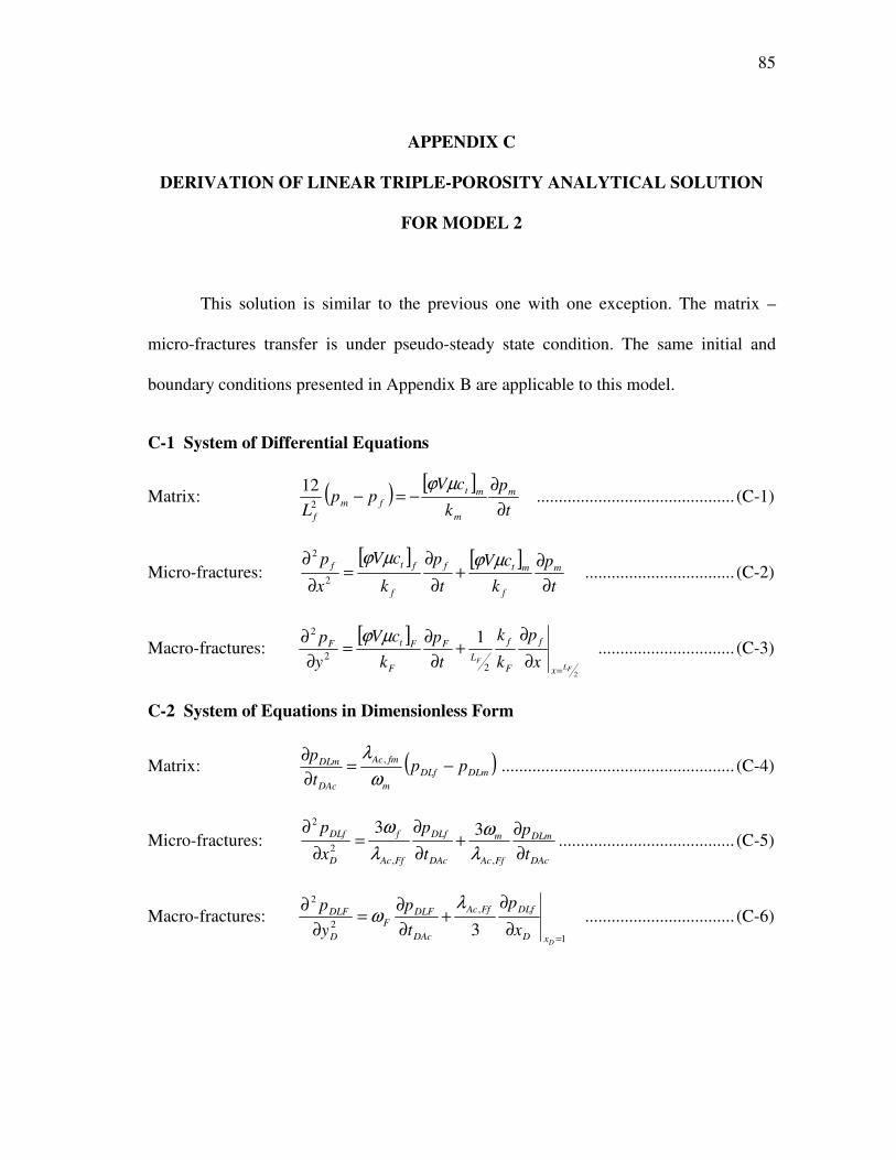
85

APPENDIX C


FOR MODEL 2

This solution is similar to the previous one with one exception. The matrix –

micro-fractures transfer is under pseudo-steady state condition. The same initial and

boundary conditions presented in Appendix B are applicable to this model.

C-1 System of Differential Equations

Matrix: ( ) [ ]t

p

k

cVpp

L

m

m

mt

fm

f ∂

∂−=−

µϕ2

12 ............................................. (C-1)

Micro-fractures: [ ] [ ]

t

p

k

cV

t

p

k

cV

x

pm

f

mtf

f

ftf

∂

∂+

∂

∂=

∂

∂ µϕµϕ2

2

.................................. (C-2)

Macro-fractures: [ ]

22

2

2 1

FLF

x

f

F

f

L

F

F

FtF

x

p

k

k

t

p

k

cV

y

p

=∂

∂+

∂

∂=

∂

∂ µϕ ............................... (C-3)

C-2 System of Equations in Dimensionless Form

Matrix: ( )DLmDLf

m

fmAc

DAc

DLm ppt

p−=

∂

∂

ω

λ , ..................................................... (C-4)

Micro-fractures: DAc

DLm

FfAc

m

DAc

DLf

FfAc

f

D

DLf

t

p

t

p

x

p

∂

∂+

∂

∂=

∂

∂

,,

2

233

λ

ω

λ

ω ........................................ (C-5)

Macro-fractures:

1

,

2

2

3=

∂

∂+

∂

∂=

∂

∂

DxD

DLfFfAc

DAc

DLFF

D

DLF

x

p

t

p

y

p λω .................................. (C-6)

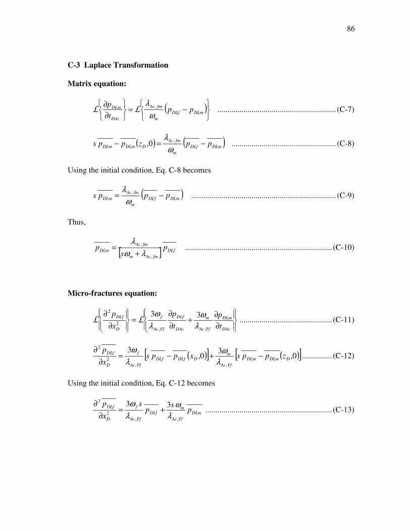
86

C-3 Laplace Transformation

Matrix equation:

( )

−=

∂

∂DLmDLf

m

fmAc

DAc

DLm ppt

p

ω

λ ,LL ........................................................... (C-7)

( ) ( )DLmDLf

m

fmAc

DDLmDLm ppzpps −=−ω

λ ,0, .................................................... (C-8)

Using the initial condition, Eq. C-8 becomes

( )DLmDLf

m

fmAc

DLm ppps −=ω

λ , ........................................................................ (C-9)

Thus,

[ ] DLf

fmAcm

fmAc

DLm ps

p,

,

λω

λ

+= ......................................................................... (C-10)


∂

∂+

∂

∂=

∂

∂

DAc

DLm

FfAc

m

DAc

DLf

FfAc

f

D

DLf

t

p

t

p

x

p

,,

2

233

λ

ω

λ

ωLL .............................................. (C-11)

( )[ ] ( )[ ]0,3

0,3

,,

2

2

DDLmDLm

FfAc

mDDLfDLf

FfAc

f

D

DLfzppsxpps

x

p−+−=

∂

∂

λ

ω

λ

ω ............... (C-12)


DLm

FfAc

mDLf

FfAc

f

D

DLfp

sp

s

x

p

,,

2

233

λ

ω

λ

ω+=

∂

∂ ............................................................... (C-13)

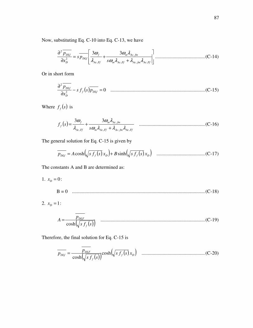
87

Now, substituting Eq. C-10 into Eq. C-13, we have

++=

∂

∂

FfAcfmAcFfAcm

fmAcm

FfAc

f

DLf

D

DLf

sps

x

p

,,,

,

,

2

2 33

λλλω

λω

λ

ω ........................................ (C-14)

Or in short form

( ) 02

2

=−∂

∂DLff

D

DLfpsfs

x

p ............................................................................ (C-15)

Where ( )sf f is

( )FfAcfmAcFfAcm

fmAcm

FfAc

f

fs

sf,,,

,

,

33

λλλω

λω

λ

ω

++= ..................................................... (C-16)

The general solution for Eq. C-15 is given by

( )( ) ( )( )DfDfDLf xsfsBxsfsAp sinhcosh += ....................................... (C-17)


1. 0=Dx :

B = 0 ........................................................................................................... (C-18)

2. 1=Dx :

( )( )sfs

pA

f

DLF

cosh= .................................................................................... (C-19)

Therefore, the final solution for Eq. C-15 is

( )( ) ( )( )Df

f

DLFDLf xsfs

sfs

pp cosh

cosh= ................................................... (C-20)

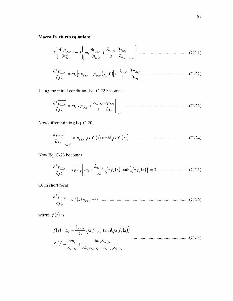
88


∂

∂+

∂

∂=

∂

∂

=1

,

2

2

3DxD

DLfFfAc

DAc

DLFF

D

DLF

x

p

t

p

y

p λωLL ............................................ (C-21)

( )[ ]1

,

2

2

30,

=∂

∂+−=

∂

∂

DxD

DLfFfAc

DDLFDLFF

D

DLF

x

pypps

y

p λω ................................... (C-22)


1

,

2

2

3=

∂

∂+=

∂

∂

DxD

DLfFfAc

DLFF

D

DLF

x

pps

y

p λω ......................................................... (C-23)

Now differentiating Eq. C-20,

( ) ( )( )sfssfspx

pffDLF

xD

DLf

D

tanh

1

=∂

∂

=

................................................. (C-24)

Now Eq. C-23 becomes

( ) ( )( ) 0tanh3

,

2

2

=

+−

∂

∂sfssfs

sps

y

pff

FfAc

FDLF

D

DLFλ

ω ........................... (C-25)

Or in short form

( ) 02

2

=−∂

∂DLF

D

DLF psfsy

p .............................................................................. (C-26)

where ( )sf is

( ) ( ) ( )( )

( )FfAcfmAcFfAcm

fmAcm

FfAc

f

f

ff

FfAc

F

ssf

sfssfss

sf

,,,

,

,

,

33

tanh3

λλλω

λω

λ

ω

λω

++=

+=

................................................ (C-53)

89

APPENDIX D


FOR MODEL 3

In this section, the triple-porosity solution is derived for the system with transient

interporosity flow between matrix and micro-fractures and pseudo-steady state flow

between the two fractures systems.

D-1 System of Differential Equations

Matrix: [ ]

t

p

k

cV

z

p m

m

mtm

∂

∂=

∂

∂ µϕ2

2

........................................................... (D-1)

Micro-fractures: ( )[ ]

22

2

112

fLf

z

m

f

m

L

f

f

ft

Ff

F z

p

k

k

t

p

k

cVpp

L =∂

∂+

∂

∂=−−

µϕ ................ (D-2)

Macro-fractures: [ ] [ ]

22

2

21

fLf

z

m

F

m

L

f

F

ftF

F

FtF

z

p

k

k

t

p

k

cV

t

p

k

cV

y

p

=∂

∂+

∂

∂+

∂

∂=

∂

∂ µϕµϕ .... (D-3)

D-2 System of Differential Equations in Dimensionless Form

Matrix: DAc

DLm

fmAc

m

D

DLm

t

p

z

p

∂

∂=

∂

∂

,

2

2 3

λ

ω ........................................................... (D-4)

Micro-fractures: ( )1,

,

, 3

1

=∂

∂+

∂

∂=−

DzD

DLm

FfAc

fmAc

DAc

DLf

FfAc

f

DLfDLFz

p

t

ppp

λ

λ

λ

ω ...................... (D-5)

Macro-fractures:

1

,

2

2

3=

∂

∂+

∂

∂+

∂

∂=

∂

∂

DzD

DLmfmAc

DAc

DLf

f

DAc

DLFF

D

DLF

z

p

t

p

t

p

y

p λωω ................. (D-6)

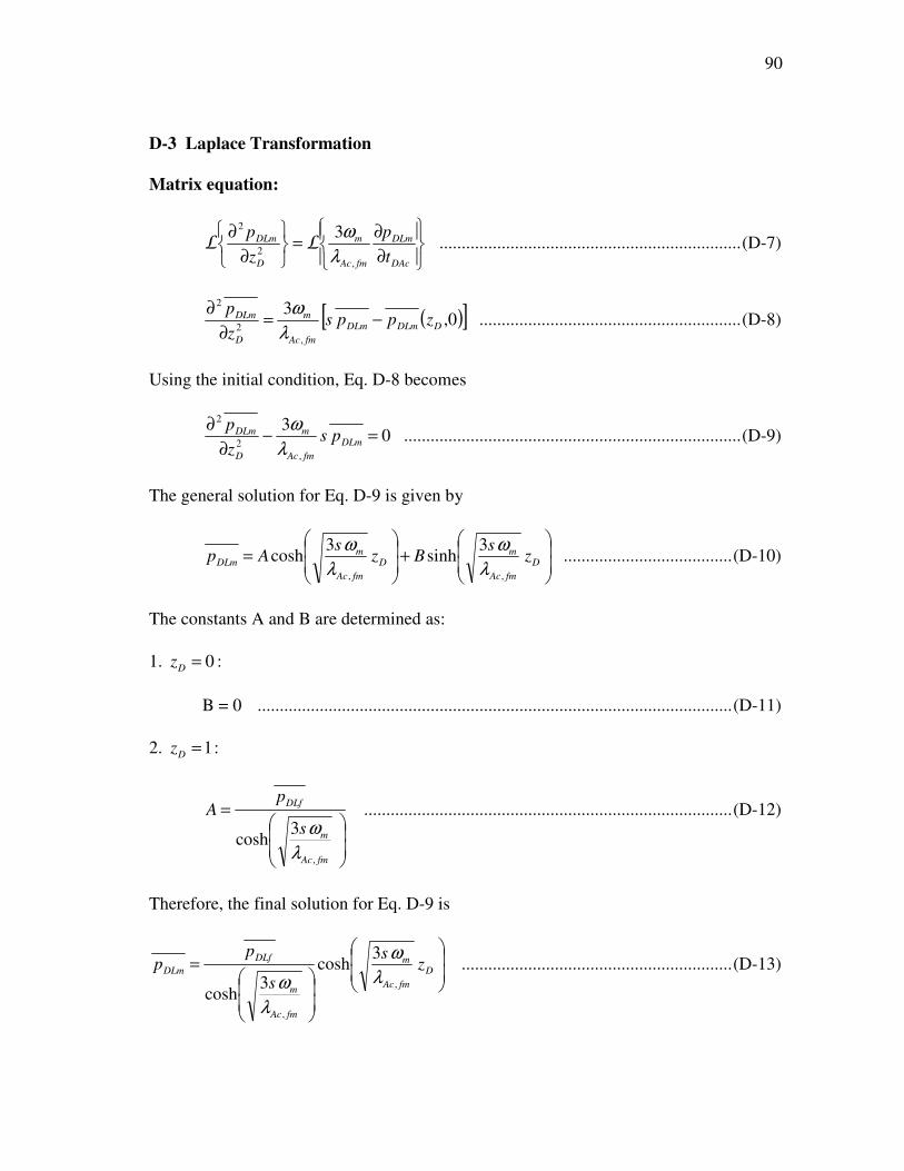
90

D-3 Laplace Transformation

Matrix equation:

∂

∂=

∂

∂

DAc

DLm

fmAc

m

D

DLm

t

p

z

p

,

2

2 3

λ

ωLL .................................................................... (D-7)

( )[ ]0,3

,

2

2

DDLmDLm

fmAc

m

D

DLm zppsz

p−=

∂

∂

λ

ω ........................................................... (D-8)

Using the initial condition, Eq. D-8 becomes

03

,

2

2

=−∂

∂DLm

fmAc

m

D

DLm psz

p

λ

ω ............................................................................ (D-9)

The general solution for Eq. D-9 is given by

+

= D

fmAc

mD

fmAc

mDLm z

sBz

sAp

,,

3sinh

3cosh

λ

ω

λ

ω ...................................... (D-10)


1. 0=Dz :

B = 0 ........................................................................................................... (D-11)

2. 1=Dz :

=

fmAc

m

DLf

s

pA

,

3cosh

λ

ω ................................................................................... (D-12)

Therefore, the final solution for Eq. D-9 is

= D

fmAc

m

fmAc

m

DLf

DLm zs

s

pp

,

,

3cosh

3cosh

λ

ω

λ

ω ............................................................. (D-13)

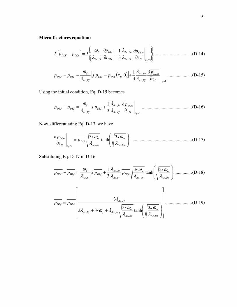
91


{ }

∂

∂+

∂

∂=−

=1,

,

, 3

1

DzD

DLm

FfAc

fmAc

DAc

DLf

FfAc

f

DLfDLFz

p

t

ppp

λ

λ

λ

ωLL ................................ (D-14)

( )[ ]1,

,

, 3

10,

=∂

∂+−=−

DzD

DLm

FfAc

fmAc

DDLfDLf

FfAc

f

DLfDLFz

pxppspp

λ

λ

λ

ω ..................... (D-15)


1,

,

, 3

1

=∂

∂+=−

DzD

DLm

FfAc

fmAc

DLf

FfAc

f

DLfDLFz

ppspp

λ

λ

λ

ω ........................................... (D-16)

Now, differentiating Eq. D-13, we have

=

∂

∂

= fmAc

m

fmAc

mDLf

zD

DLm ssp

z

p

D,,1

3tanh

3

λ

ω

λ

ω ................................................... (D-17)

Substituting Eq. D-17 in D-16

+=−

fmAc

m

fmAc

mDLf

FfAc

fmAc

DLf

FfAc

f

DLfDLF

ssppspp

,,,

,

,

3tanh

3

3

1

λ

ω

λ

ω

λ

λ

λ

ω ................ (D-18)

++

=

fmAc

m

fmAc

mfmAcfFfAc

FfAc

DLFDLf

sss

pp

,,

,,

,

3tanh

333

3

λ

ω

λ

ωλωλ

λ ....................... (D-19)

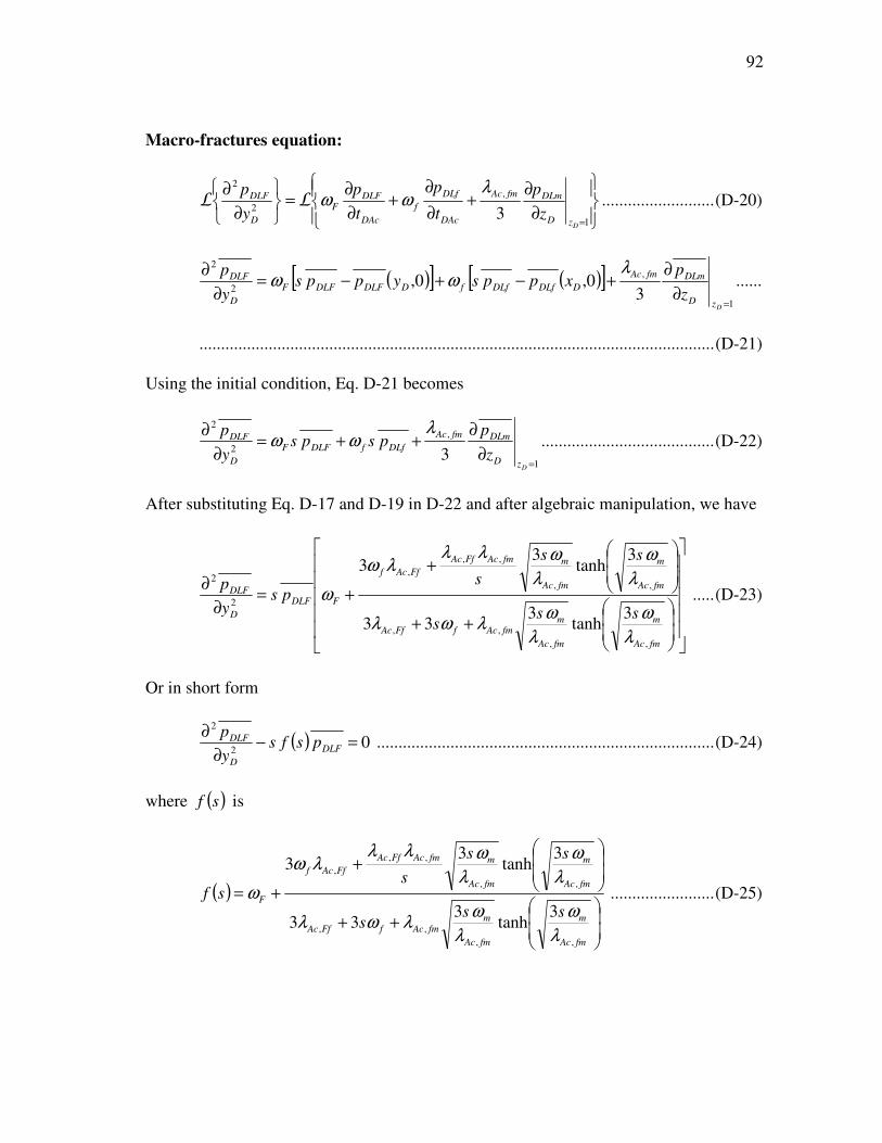
92


∂

∂+

∂

∂+

∂

∂=

∂

∂

=1

,

2

2

3DzD

DLmfmAc

DAc

DLf

f

DAc

DLFF

D

DLF

z

p

t

p

t

p

y

p λωωLL .......................... (D-20)

( )[ ] ( )[ ]1

,

2

2

30,0,

=∂

∂+−+−=

∂

∂

DzD

DLmfmAc

DDLfDLffDDLFDLFF

D

DLF

z

pxppsypps

y

p λωω ......

....................................................................................................................... (D-21)


1

,

2

2

3=

∂

∂++=

∂

∂

DzD

DLmfmAc

DLffDLFF

D

DLF

z

ppsps

y

p λωω ........................................ (D-22)

After substituting Eq. D-17 and D-19 in D-22 and after algebraic manipulation, we have

++

+

+=∂

∂

fmAc

m

fmAc

mfmAcfFfAc

fmAc

m

fmAc

mfmAcFfAc

FfAcf

FDLF

D

DLF

sss

ss

sps

y

p

,,

,,

,,

,,

,

2

2

3tanh

333

3tanh

33

λ

ω

λ

ωλωλ

λ

ω

λ

ωλλλω

ω ..... (D-23)

Or in short form

( ) 02

2

=−∂

∂DLF

D

DLF psfsy

p .............................................................................. (D-24)

where ( )sf is

( )

++

+

+=

fmAc

m

fmAc

mfmAcfFfAc

fmAc

m

fmAc

mfmAcFfAc

FfAcf

F

sss

ss

ssf

,,

,,

,,

,,

,

3tanh

333

3tanh

33

λ

ω

λ

ωλωλ

λ

ω

λ

ωλλλω

ω ........................ (D-25)

93

APPENDIX E


FOR FULLY PSEUDOSTEADY STATE FLUID TRANSFER– MODEL 4

In this section, the triple-porosity solution is derived for a system with

pseudosteady state interporosity flow between matrix and micro-fractures the two

fractures systems.

E-1 System of Differential Equations

Matrix: ( ) [ ]t

p

k

cVpp

L

m

m

mt

fm

f ∂

∂−=−

µϕ2

12 .............................................. (E-1)

Micro-fractures: ( ) [ ] [ ]t

p

k

cV

t

p

k

cVpp

L

f

f

ftm

f

mt

Ff

f ∂

∂+

∂

∂=−−

µϕµϕ2

12 ..................... (E-2)

Macro-fractures: [ ] [ ] [ ]

t

p

k

cV

t

p

k

cV

t

p

k

cV

y

p F

F

Ftf

F

ftm

F

mtF

∂

∂+

∂

∂+

∂

∂=

∂

∂ µϕµϕµϕ2

2

......... (E-3)

E-2 System of Differential Equations in Dimensionless Form

Matrix: ( )DLmDLf

m

fmAc

DAc

DLm ppt

p−=

∂

∂

ω

λ , ........................................................ (E-4)

Micro-fractures: ( )DAc

DLm

f

mDLfDLF

f

FfAc

DAc

DLf

t

ppp

t

p

∂

∂−−=

∂

∂

ω

ω

ω

λ , ...................................... (E-5)

Macro-fractures: DAc

DLFF

DAc

DLf

f

DAc

DLmm

D

DLF

t

p

t

p

t

p

y

p

∂

∂+

∂

∂+

∂

∂=

∂

∂ωωω

2

2

............................... (E-6)

94

E-3 Laplace Transformation

Matrix equation:

( )

−=

∂

∂DLmDLf

m

fmAc

DAc

DLm ppt

p

ω

λ ,LL ........................................................... (E-7)

( ) ( )DLmDLf

m

fmAc

DDLmDLm ppzpps −=−ω

λ ,0, .................................................... (E-8)

Using the initial condition, Eq. E-8 becomes

( )DLmDLf

m

fmAc

DLm ppps −=ω

λ , ........................................................................ (E-9)

Thus,

[ ] DLf

fmAcm

fmAc

DLm ps

p,

,

λω

λ

+= ......................................................................... (E-10)


( )

∂

∂−−=

∂

∂

DAc

DLm

f

mDLfDLF

f

FfAc

DAc

DLf

t

ppp

t

p

ω

ω

ω

λ ,LL ......................................... (E-11)

( ) ( ) ( )[ ]0,0,,

DDLmDLm

f

mDLfDLF

f

FfAc

DDLfDLf zppsppxpps −−−=−ω

ω

ω

λ ......... (E-12)


( ) DLm

f

mDLfDLF

f

FfAc

DLf pspppsω

ω

ω

λ−−=

, ...................................................... (E-13)

95

Substituting Eq. E-10 in E-13 and after algebraic manipulation, we have

( ) [ ] DLf

fmAcm

fmAc

f

mDLfDLF

f

FfAc

DLf ps

sppps,

,,

λω

λ

ω

ω

ω

λ

+−−= ................................. (E-14)

( )( )( ) DLF

fmAcmfmAcmfFfAc

fmAcmFfAc

DLf psss

sp

+++

+=

,,,

,,

λωλωωλ

λωλ ................................. (E-15)


∂

∂+

∂

∂+

∂

∂=

∂

∂

DAc

DLFF

DAc

DLf

f

DAc

DLmm

D

DLF

t

p

t

p

t

p

y

pωωωLL

2

2

.................................... (E-16)

( )[ ] ( )[ ] ( )[ ]0,0,0,2

2

DDLFDLFFDDLfDLffDDLmDLmm

D

DLF yppsxppszppsy

p−+−+−=

∂

∂ωωω

....................................................................................................................... (E-17)


[ ] [ ] [ ]DLFFDLffDLmm

D

DLF pspspsy

pωωω ++=

∂

∂2

2

............................................... (E-18)

Now substituting Eq. E-10 and E-15 in E-18,

( )[ ]( )

( )( ) DLFFDLF

fmAcmfmAcmfFfAc

fmAcmFfAcf

DLf

fmAcFf

fmAc

m

D

DLF

pspssss

s

pssy

p

ωλωλωωλ

λωλω

λωω

λω

++++

++

+−−=

∂

∂

,,,

,,

,

,

2

2

1 ......... (E-19)

( )( )( )

+++

+++=

∂

∂

fmAcmfmAcmfFfAc

fmAcmFfAcfFfAcfmAcm

FDLF

D

DLF

sss

sps

y

p

,,,

,,,,

2

2

λωλωωλ

λωλωλλωω .............. (E-20)

( )[ ]( )( )

+++

+++=

∂

∂

fmAcmfmAcmfFfAc

fmAcmffmAcmFfAc

FDLF

D

DLF

sss

sps

y

p

,,,

,,,

2

2

λωλωωλ

λωωλωλω .............. (E-21)

96

Or in short form

( ) 02

2

=−∂

∂DLF

D

DLF psfsy

p ............................................................................ (E-22)

where ( )sf is

( )( )[ ]


fmAcmffmAcmFfAc

Fsss

ssf

,,,

,,,

λωλωωλ

λωωλωλω

+++

+++= ................................ (E-23)

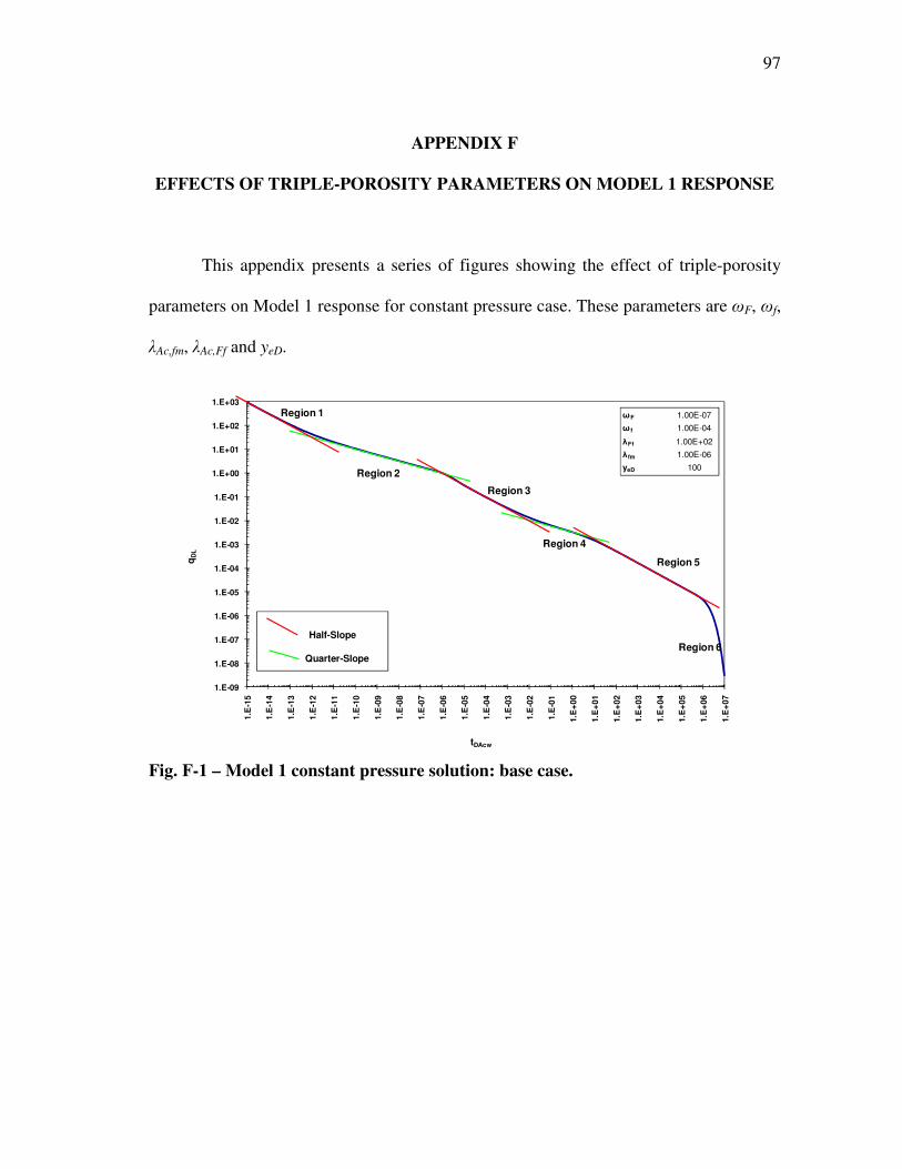
97

APPENDIX F

EFFECTS OF TRIPLE-POROSITY PARAMETERS ON MODEL 1 RESPONSE

This appendix presents a series of figures showing the effect of triple-porosity

parameters on Model 1 response for constant pressure case. These parameters are ωF, ωf,

λAc,fm, λAc,Ff and yeD.

1.E-09

1.E-08

1.E-07

1.E-06

1.E-05

1.E-04

1.E-03

1.E-02

1.E-01

1.E+00

1.E+01

1.E+02

1.E+03

1.E

-15

1.E

-14

1.E

-13

1.E

-12

1.E

-11

1.E

-10

1.E

-09

1.E

-08

1.E

-07

1.E

-06

1.E

-05

1.E

-04

1.E

-03

1.E

-02

1.E

-01

1.E

+00

1.E

+01

1.E

+02

1.E

+03

1.E

+04

1.E

+05

1.E

+06

1.E

+07

qD

L

tDAcw

ωF 1.00E-07

ω f 1.00E-04

λFf 1.00E+02

λfm 1.00E-06

yeD 100

Region 1

Region 2

Region 3

Region 4

Region 5

Region 6

Half-Slope

Quarter-Slope

Fig. F-1 – Model 1 constant pressure solution: base case.

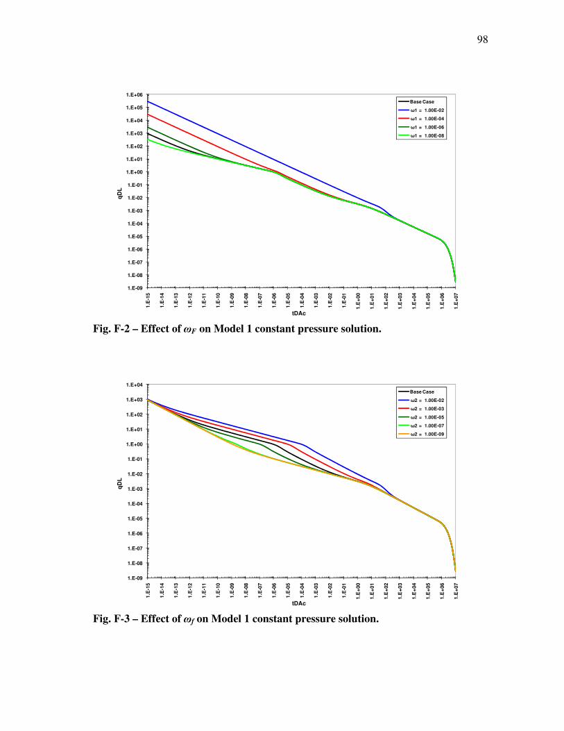
98

1.E-09

1.E-08

1.E-07

1.E-06

1.E-05

1.E-04

1.E-03

1.E-02

1.E-01

1.E+00

1.E+01

1.E+02

1.E+03

1.E+04

1.E+05

1.E+06

1.E

-15

1.E

-14

1.E

-13

1.E

-12

1.E

-11

1.E

-10

1.E

-09

1.E

-08

1.E

-07

1.E

-06

1.E

-05

1.E

-04

1.E

-03

1.E

-02

1.E

-01

1.E

+00

1.E

+01

1.E

+02

1.E

+03

1.E

+04

1.E

+05

1.E

+06

1.E

+07

qD

L

tDAc

Base Case

ω1 = 1.00E-02

ω1 = 1.00E-04

ω1 = 1.00E-06

ω1 = 1.00E-08

Fig. F-2 – Effect of ωF on Model 1 constant pressure solution.

1.E-09

1.E-08

1.E-07

1.E-06

1.E-05

1.E-04

1.E-03

1.E-02

1.E-01

1.E+00

1.E+01

1.E+02

1.E+03

1.E+04

1.E

-15

1.E

-14

1.E

-13

1.E

-12

1.E

-11

1.E

-10

1.E

-09

1.E

-08

1.E

-07

1.E

-06

1.E

-05

1.E

-04

1.E

-03

1.E

-02

1.E

-01

1.E

+00

1.E

+01

1.E

+02

1.E

+03

1.E

+04

1.E

+05

1.E

+06

1.E

+07

qD

L

tDAc

Base Case

ω2 = 1.00E-02

ω2 = 1.00E-03

ω2 = 1.00E-05

ω2 = 1.00E-07

ω2 = 1.00E-09

Fig. F-3 – Effect of ωf on Model 1 constant pressure solution.

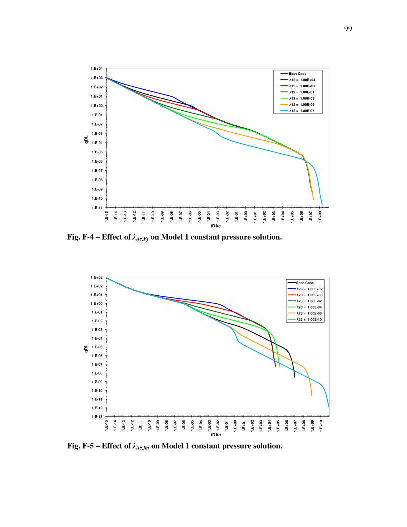
99

1.E-11

1.E-10

1.E-09

1.E-08

1.E-07

1.E-06

1.E-05

1.E-04

1.E-03

1.E-02

1.E-01

1.E+00

1.E+01

1.E+02

1.E+03

1.E+04

1.E

-15

1.E

-14

1.E

-13

1.E

-12

1.E

-11

1.E

-10

1.E

-09

1.E

-08

1.E

-07

1.E

-06

1.E

-05

1.E

-04

1.E

-03

1.E

-02

1.E

-01

1.E

+00

1.E

+01

1.E

+02

1.E

+03

1.E

+04

1.E

+05

1.E

+06

1.E

+07

1.E

+08

qD

L

tDAc

Base Case

λ12 = 1.00E+04

λ12 = 1.00E+01

λ12 = 1.00E-01

λ12 = 1.00E-03

λ12 = 1.00E-05

λ12 = 1.00E-07

Fig. F-4 – Effect of λAc,Ff on Model 1 constant pressure solution.

1.E-13

1.E-12

1.E-11

1.E-10

1.E-09

1.E-08

1.E-07

1.E-06

1.E-05

1.E-04

1.E-03

1.E-02

1.E-01

1.E+00

1.E+01

1.E+02

1.E+03

1.E

-15

1.E

-14

1.E

-13

1.E

-12

1.E

-11

1.E

-10

1.E

-09

1.E

-08

1.E

-07

1.E

-06

1.E

-05

1.E

-04

1.E

-03

1.E

-02

1.E

-01

1.E

+00

1.E

+01

1.E

+02

1.E

+03

1.E

+04

1.E

+05

1.E

+06

1.E

+07

1.E

+08

1.E

+09

1.E

+10

qD

L

tDAc

Base Case

λ23 = 1.00E+02

λ23 = 1.00E+00

λ23 = 1.00E-02

λ23 = 1.00E-04

λ23 = 1.00E-08

λ23 = 1.00E-10

Fig. F-5 – Effect of λAc,fm on Model 1 constant pressure solution.

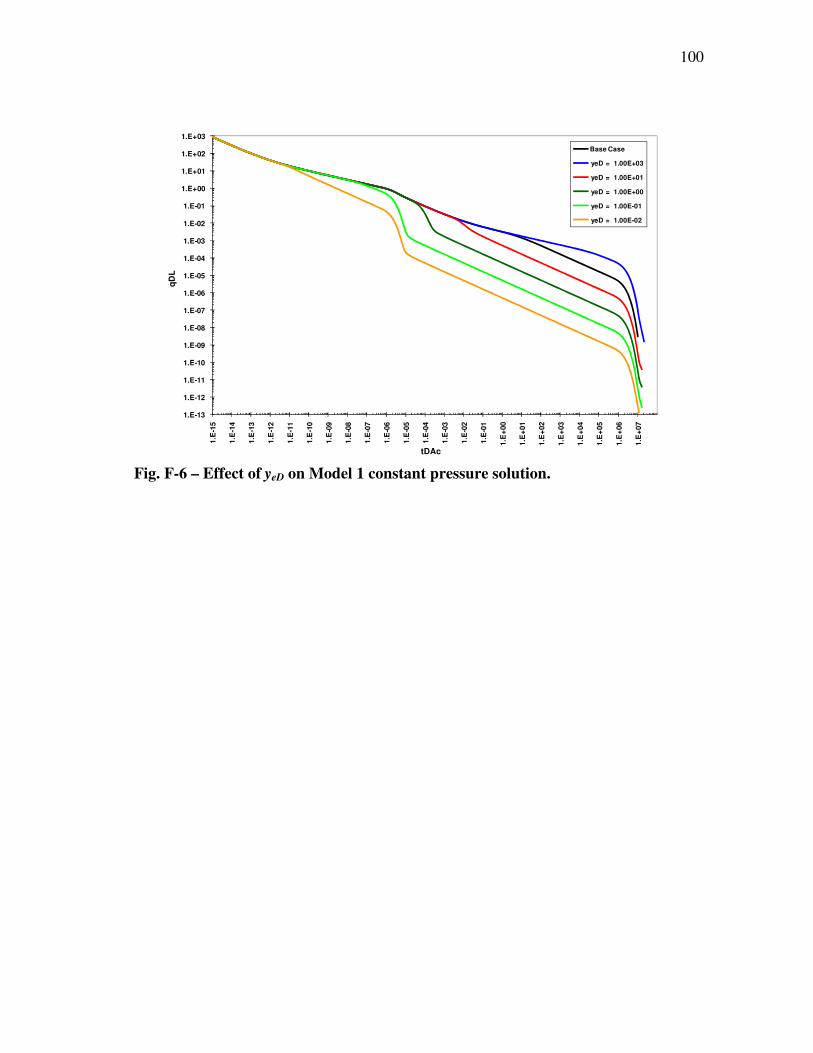
100

1.E-13

1.E-12

1.E-11

1.E-10

1.E-09

1.E-08

1.E-07

1.E-06

1.E-05

1.E-04

1.E-03

1.E-02

1.E-01

1.E+00

1.E+01

1.E+02

1.E+03

1.E

-15

1.E

-14

1.E

-13

1.E

-12

1.E

-11

1.E

-10

1.E

-09

1.E

-08

1.E

-07

1.E

-06

1.E

-05

1.E

-04

1.E

-03

1.E

-02

1.E

-01

1.E

+00

1.E

+01

1.E

+02

1.E

+03

1.E

+04

1.E

+05

1.E

+06

1.E

+07

qD

L

tDAc

Base Case

yeD = 1.00E+03

yeD = 1.00E+01

yeD = 1.00E+00

yeD = 1.00E-01

yeD = 1.00E-02

Fig. F-6 – Effect of yeD on Model 1 constant pressure solution.

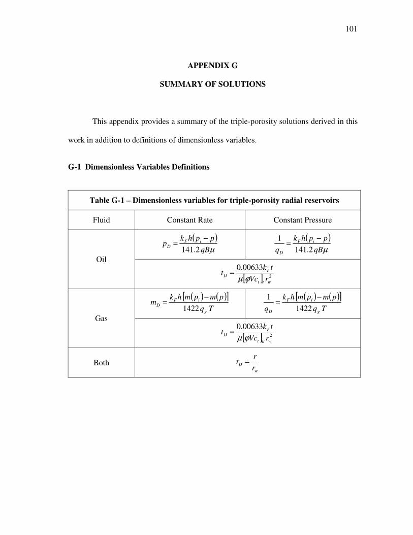
101

APPENDIX G

SUMMARY OF SOLUTIONS

This appendix provides a summary of the triple-porosity solutions derived in this

work in addition to definitions of dimensionless variables.

G-1 Dimensionless Variables Definitions

Table G-1 – Dimensionless variables for triple-porosity radial reservoirs

Fluid Constant Rate Constant Pressure

Oil

( )µqB

pphkp iF

D2.141

−=

( )µqB

pphk

q

iF

D 2.141

1 −=

[ ] 2

00633.0

wtt

FD

rVc

tkt

ϕµ=

Gas

( ) ( )[ ]Tq

pmpmhkm

g

iFD

1422

−=

( ) ( )[ ]Tq

pmpmhk

q g

iF

D 1422

1 −=

[ ] 2

00633.0

wtit

FD

rVc

tkt

ϕµ=

Both w

Dr

rr =

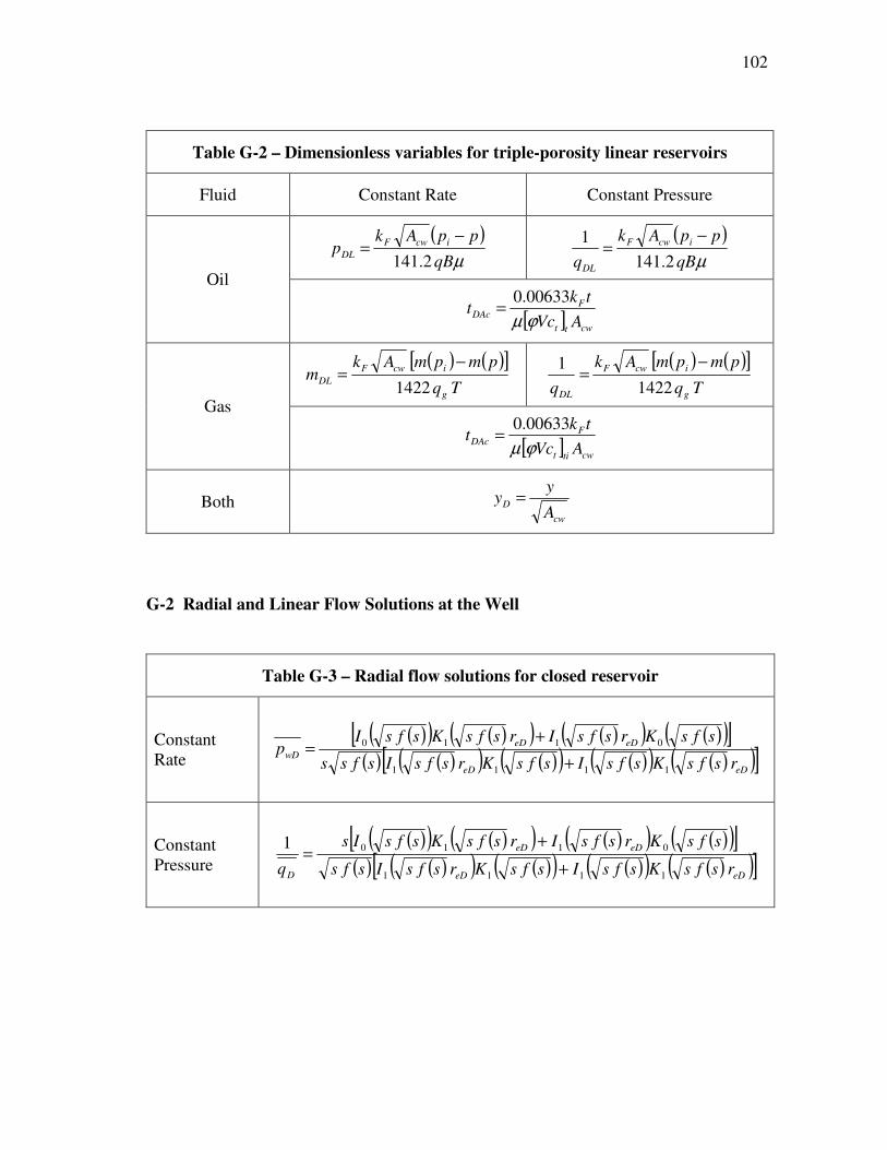
102

Table G-2 – Dimensionless variables for triple-porosity linear reservoirs

Fluid Constant Rate Constant Pressure

Oil

( )µqB

ppAkp

icwF

DL2.141

−=

( )µqB

ppAk

q

icwF

DL 2.141

1 −=

[ ] cwtt

FDAc

AVc

tkt

ϕµ

00633.0=

Gas

( ) ( )[ ]Tq

pmpmAkm

g

icwF

DL1422

−=

( ) ( )[ ]Tq

pmpmAk

q g

icwF

DL 1422

1 −=

[ ] cwtit

FDAc

AVc

tkt

ϕµ

00633.0=

Both cw

DA

yy =

G-2 Radial and Linear Flow Solutions at the Well

Table G-3 – Radial flow solutions for closed reservoir

Constant

Rate

( )( ) ( )( ) ( )( ) ( )( )[ ]( ) ( )( ) ( )( ) ( )( ) ( )( )[ ]eDeD

eDeD

wDrsfsKsfsIsfsKrsfsIsfss

sfsKrsfsIrsfsKsfsIp

1111

0110

+

+=

Constant

Pressure

( )( ) ( )( ) ( )( ) ( )( )[ ]( ) ( )( ) ( )( ) ( )( ) ( )( )[ ]eDeD

eDeD

D rsfsKsfsIsfsKrsfsIsfs

sfsKrsfsIrsfsKsfsIs

q1111

01101

+

+=

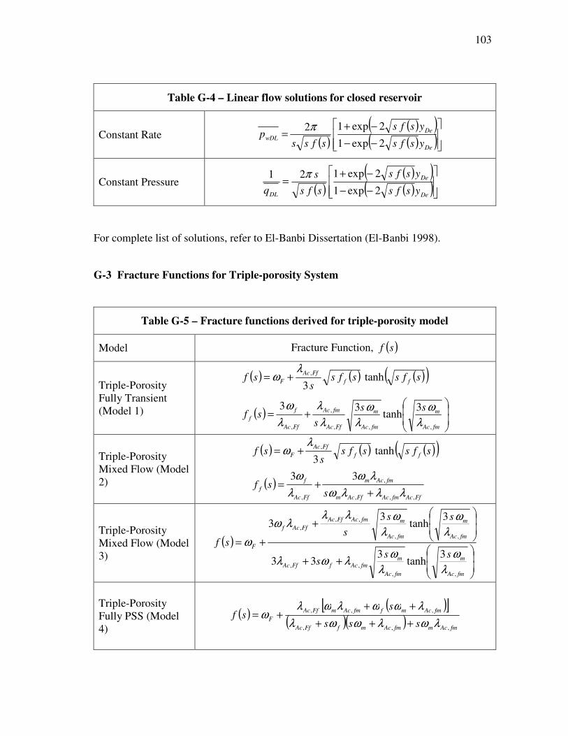
103

Table G-4 – Linear flow solutions for closed reservoir

Constant Rate ( )

( )( )( )( )

−−

−+=

De

De

wDLysfs

ysfs

sfssp

2exp1

2exp12π

Constant Pressure ( )

( )( )( )( )

−−

−+=

De

De

DL ysfs

ysfs

sfs

s

q 2exp1

2exp121 π

For complete list of solutions, refer to El-Banbi Dissertation (El-Banbi 1998).

G-3 Fracture Functions for Triple-porosity System

Table G-5 – Fracture functions derived for triple-porosity model

Model Fracture Function, ( )sf

Triple-Porosity

Fully Transient

(Model 1)

( ) ( ) ( )( )

( )

+=

+=

fmAc

m

fmAc

m

FfAc

fmAc

FfAc

f

f

ff

FfAc

F

ss

ssf

sfssfss

sf

,,,

,

,

,

3tanh

33

tanh3

λ

ω

λ

ω

λ

λ

λ

ω

λω

Triple-Porosity

Mixed Flow (Model

2)

( ) ( ) ( )( )

( )FfAcfmAcFfAcm

fmAcm

FfAc

f

f

ff

FfAc

F

ssf

sfssfss

sf

,,,

,

,

,

33

tanh3

λλλω

λω

λ

ω

λω

++=

+=

Triple-Porosity

Mixed Flow (Model

3)

( )

++

+

+=

fmAc

m

fmAc

mfmAcfFfAc

fmAc

m

fmAc

mfmAcFfAc

FfAcf

F

sss

ss

ssf

,,

,,

,,

,,

,

3tanh

333

3tanh

33

λ

ω

λ

ωλωλ

λ

ω

λ

ωλλλω

ω

Triple-Porosity

Fully PSS (Model

4)

( )( )[ ]


fmAcmffmAcmFfAc

Fsss

ssf

,,,

,,,

λωλωωλ

λωωλωλω

+++

+++=

104

VITA

Name: Hasan Ali Alahmadi

Address: P.O. Box 13970

Saudi Aramco

Dhahran 31311

Saudi Arabia

Email Address: [email protected]

Education: B.Sc., Petroleum Engineering, King Fahd University of Petroleum &

Minerals (KFUPM), Saudi Arabia, 2005

M.S., Petroleum Engineering, Texas A&M University, 2010

a triple-porosity model for fractured horizontal wells

Documents