big data mining using supervised machine learning ... · pdf filebig data is defined as large...
TRANSCRIPT

International Journal of Computational Intelligence Research
ISSN 0973-1873 Volume 13, Number 8 (2017), pp. 2095-2111
© Research India Publications
http://www.ripublication.com
Big data mining using supervised machine learning
approaches for Hadoop with Weka distribution
Anuja Jain Varsha Sharma Vivek Sharma
SOIT, Bhopal SOIT, Bhopal SOIT, Bhopal
Abstract
Data is increasing very rapidly with the increase in technologies. To process
this data and performing accurate mining to yield conclusions is a challenge.
This domain to process and mining this big data is termed as big data mining.
To store and process big data many open source tools were proposed and are
present in Apache foundation. Apache Hadoop is the most widely used tool
for big data processing. Apache Hadoop consists of two main components
namely Hadoop distributed file system (HDFS) and map/reduce. HDFS is
used to store the data in distributed form and map/reduce is used to process
this distributed spread data. In the past many data mining and classification
approaches have been proposed for big data in which for implementing
machine learning no standard tool is used. And no generic topology for data
flow is proposed to implement such model. And accuracy of classification for
raw dataset is also poor. In this dissertation to perform big data mining Apache
Hadoop and Weka is used. Weka is an open source tool for machine learning
proposed by Waikato university of New Zealand. Here in this work Apache
Hadoop is connected with Weka. Using this combination big data is stored on
HDFS and processed using Weka using Knowledge flow of Weka. Knowledge
flow provides a means to construct topologies using them HDFS components
can be used to provide data to machine learning algorithms provided in Weka.
In this work supervised machine learning approaches which include Naïve
Bayes, Support vector machine, J48 are used for big data mining. The
accuracy of these approaches is compared for raw data and normalized data
given to the same topology. It is found proposed approach for big data mining
yields better results as compared to the reference approach.
Keywords: Hadoop, Weka, Supervised machine learning.
2096 Anuja Jain, Varsha Sharma and Vivek Sharma
I. INTRODUCTION
Big data is defined as large quantity of data which have need of new technologies and
architecture to make possible to extort value from it by capturing and analysis
process. New sources of big data include location specific data whichhas arrived from
traffic management and from the tracking of personal devices such as Smartphone’s.
Big data has come into view because we are living inthe world which makes
mounting use of data intensive technologies. Due to such large size of data it becomes
very difficult to achieve effective analysis using existingtraditional techniques.
Since Big data is new upcoming technology in the market which can bring the huge
benefits to the business organizations, it becomes necessary various challenges and
issues associated in bringing and adopting to this technology are need to be
understand. Big data concept means a dataset which continues grew so much that it
becomes difficult to manage it using existing database models and tools. So at last Big
data is data that exceeds the processing capacity of conventional database systems.
The data is huge sized, moves too fast, or doesn’t fit the structures of our database
architectures. To gain value from this data, you must choose a substitute way to
process it.
What are the problems?
There are many problems to handle big data like storage, processing etc.
a) Data integration – The structure of merging data is not so easy task with a
reasonable cost.
b) Data volume – The ability to process the volume at a suitable rate so that the
information is available to result analysers when they need it.
c) Skills availability –There are shortage of people. Who have the proficiency to
bring all data mutually, analyse it and publish the results.
d) Solution cost –To ensure a positive ROI on a Big Data project; it is crucial to
reduce the cost of the solutions.
What are the solutions?
Big data is very difficult to process and store. Mainly Hadoop is used to process the
big data. Hadoop used HDFS to store the data efficiently and MapReduce framework
for processing the data. MPI is also used to process the big data.
Big data define as the pool ofinformation’s that is unable to handled or analysed using
an existing or traditional data mining techniques or the tools. Constantly increase of
computational power has brought tremendous flow of data in the past two decades.
This remarkable flow of data is called as “big data” it cannot be deal with the aid of
existing tools or any other procedure and this is more comprehensible to computers.
Big data mining using supervised machine learning approaches for Hadoop… 2097
The size of BigData range from petabytes (PB) to Exabyte’s (EB) or to zettabytes
(ZB).The BigData created from the client server interaction which is known as
customer call records or transaction histories etc.
Big Data system is getting lot of importance now a day from organisations to handle
those data as well as using them in business growth.Some Big data examples such as
data from Finance, Internet, Mobile device, Radio – Frequency Identification (RFID),
Science, Sensor and Streaming are the top most seven data drivers.
BIG DATA HANDLING TOOLS
Hadoop
Hadoop is an Apache open source framework which supports java and also java code
for implementation that allows distributed processing of large records across clusters
of computers using easy programming models. The Hadoop framework application
moving in an atmosphere that offer distributed storage and estimation across clusters
of computers. Hadoop is made for level up from single server to thousands of
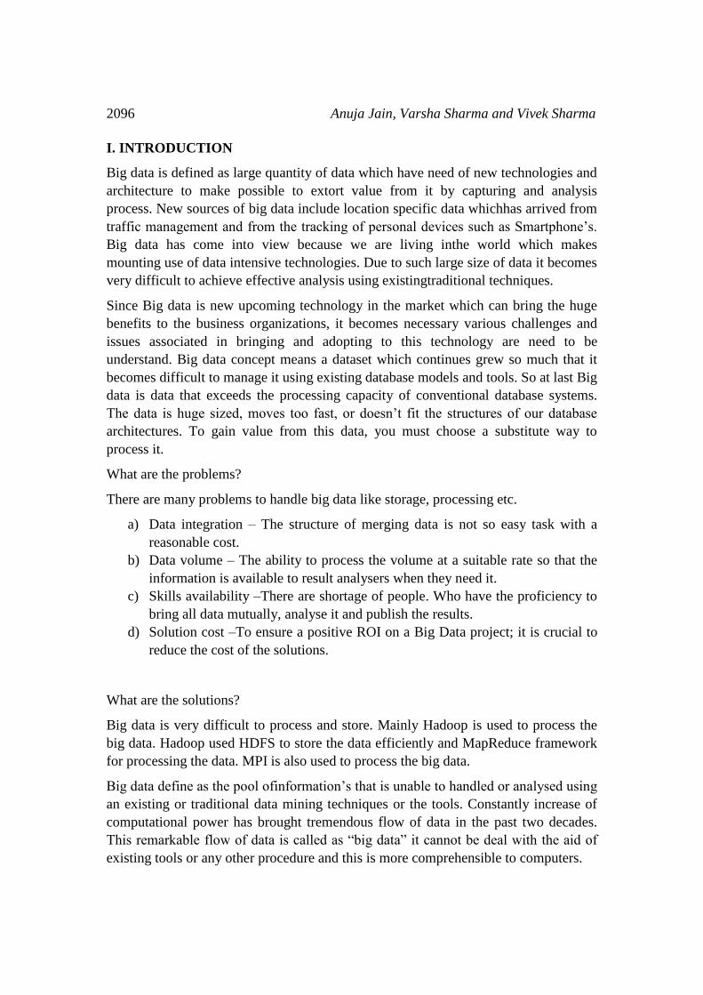
equipment, each offering local calculation and storage [12].
Figure: Architecture of Hadoop
Hadoop mainly consist of 2 components.
MapReduce
MapReduce applications can precede multiple terabytes of data in parallel on large
clusters in a fault-tolerant manner and reliable. MapReduce is an estimation paradigm
in which a function is divided into self-reliant units of work. Each of these units of
process can be issued on any node in the cluster.
A MapReduce job divides the input data into several chunks that are processed by
map jobs in similar way. The framework arranges the map outputs, which are then
input to reduce tasks. Task’s inputs and outputs are lain up in the file system. The
Common
utilities
YARN
framework
HDFS
MapReduce
2098 Anuja Jain, Varsha Sharma and Vivek Sharma
MapReduce framework and the HDFS (Hadoop Distributed File System) are
classically on the same set of nodes, which allow the structure to schedule tasks on
nodes that hold data [13].
The MapReduce framework having a single key Job Tracker and one secondary Task
Tracker per node. The main node plan for job section tasks, re-executes, and monitors
tasks abortive tasks. The secondary node processes as directed by the primary node.
MapReduce have two phases
The map phase
The map section is the 1st a part of the data process sequence inside the MapReduce
framework. Map functions serve as worker nodes which will process many smaller
snippets of the whole data set. The MapReduce framework is liable for dividing the
data set input into smaller chunks, and feeding them to a corresponding map function.
after you write a map function, there's no got to incorporate logic to change the
function to form multiple maps which will use the distributed computing design of
Hadoop. These functions are oblivious to each data volume and also the cluster during
which they're operative. As such, they'll be used unchanged for each little and huge
data sets (which is commonest for those that are victimization Hadoop) [11].
The reduce phase
As with the map function, developers additionally should produce a reduce function.
The key/value pairs from map outputs should correspond to the acceptable reducer
partition such the ultimate results are aggregates of the suitably corresponding data.
once the shuffle method is completed and therefore the reducer copies all of the map
task outputs, the reducers will get into what's called a merge method. throughout this a
part of the reduce part, all map outputs will be incorporate along to keep up their type
ordering that's established throughout the map part. once the ultimate merge is
complete then this reduce task of consolidating results for each key at intervals the
incorporate output (and the ultimate result set), is written to the disk on the HDFS
[11].
Data mining is that the extraction of knowledge from great deal of observational data
sets, to seek out surprising relationship and pattern hidden in data, summarize the data
in novel ways that during which to make it comprehendible and useful to the data
users [1,2]. Web usage mining is that the appliance of data mining technique to
automatically discover and extract useful information from a particular pc [2,3]. There
are many major data processing techniques
Classification: Classification may be a one in all the classical data processing
techniques that is predicated on machine learning. Essentially classification is applied

Big data mining using supervised machine learning approaches for Hadoop… 2099
to classify every item during a set of information into one in all predefined set of
categories. Classification technique makes use of many mathematical techniques like
linear programming, call trees, neural network and statistics.
Clustering: It is an unsupervised data mining technique that makes effective and
helpful clusters, which useful and meaningful also. Cluster of objects which have
similar characteristics using different clustering technique. The clustering technique
specifies the classes and put objects in each class to whom they belong, while in the
classification techniques, objects are assigned according to predefined classes.
Association: Association is one of the well-known data mining technique. In
association, a pattern is found out based on a relationship between items in the same
transaction. That’s why association technique is also known as relation technique.
Prediction: The prediction, as it name suggest, is one of a data mining techniques that
seeks to discover relationship between independent variables as well as relationship
between dependent and independent variables.
Sequential Patterns: Sequential patterns analysis is one of data mining technique that
tries to find or identify similar patterns, trends or regular events in transaction data
over a business period.
Decision trees: Decision tree is one of the most frequently used data mining
techniques because its model is easy to interpret for users. In decision tree technique,
structure of decision tree is such that the very first point is root, which is a simple
condition or question that has multiple answers. Each answer then further leads us to a
set of conditions or questions that help us found out the data on the basis of which we
can make the final decision depending on it.
II. MACHINE LEARNING
In this section past many approaches for data classification have been proposed.
Which includes Naïve bayes, Support vector machine, Random Forest, Decision tree,
PART and all these methods are compared in table 1. Which consists of related work
done in the past.
Machine learning may be a kind of AI (AI) that gives computers with the power to
learn while not being expressly programmed. Machine learning focuses on the event
of computer programs which will change once exposed to new information.
Machine learning tasks are generally classified into 3 broad classes, looking on the
character of the learning "signal" or "feedback" offered to a learning system. These
are[14]
• Supervised learning: the computer is bestowed with example inputs and
their desired outputs, given by a "teacher", and also the goal is to learn a

2100 Anuja Jain, Varsha Sharma and Vivek Sharma
general rule that maps inputs to outputs.
• Unsupervised learning: No labels are given to the learning rule, going
away it on its own to search out structure in its input. unsupervised
learning will be a goal in itself (discovering hidden patterns in data) or a
way towards an finish (feature learning).
• Reinforcement learning: A computer program interacts with a dynamic
setting within which it should perform a precise goal (such as driving a
vehicle or taking part in a game against an opponent [4]). The program is
provided feedback in terms of rewards and punishments because it
navigates its drawback area.
Bayes Classifier— It originates from previous works in pattern recognition and is
joined to the family of probabilistic Graphical Models. For every category, a
probabilistic outline is hold on. The chance of every attribute and also the probability
of the category are keep during this outline. The graphical models are wont to show
data concerning domains that are unsure in nature. Within the graphs [15], nodes
depict variables and also the edges that connect corresponding random variable nodes
are appointed weights that represent probabilistic dependencies. On encountering a
brand new instance, the rule simply creates an update of the chances keep in
conjunction with the particular category [12]. The sequence of training instances and
also the existence of classification errors don't have any role during this method. So
primarily it's to predict the category looking on the worth of the members of the
category. This class consists of thirteen classifiers, however solely three of these are
compatible with our chosen dataset.
Function classifier— It deploys the concept of regression and neural network. input
data is mapped to the output. It employs the repetitive parameter estimation theme.
Overall there are eighteen classifiers beneath this class, out of that only 2 are
compatible with our dataset.
The main Objectives of this analysis includes:
A. huge data analysis using Apache Hadoop.
B. correct classification of this huge data using supervised machine learning.
C. Apache Hadoop and weka are going to be used for that huge information
classification.
D. improvement in accuracy of classification over this dataset using correct
discretization technique.
E. to possess high accuracy, True positive rate and preciseness and low false
positive rate.
To evaluate the performance of the supervised machine learning approaches four
analysis metrics are thought of. These are:
A. Accuracy – Accuracy will be outlined as properly classified instances divided

Big data mining using supervised machine learning approaches for Hadoop… 2101
by the full variety of instances in dataset.
B. preciseness - preciseness could be a measurement of what number of the
properly classified instances that are relevant, i.e. it's a extremely specific
metric that's best discovered in relevance different metrics like recall and
accuracy.
C. True positive rate (TP) - variety of examples predicted positive that are
literally positive.
D. False Positive rate (FP) - variety of examples foreseen positive that are
literally negative.
Table 1
COMPARISON OF CLASSIFIERS
CLASSIFIER CATEGORY DESCRIPTION REFERENCE
Naive Bayes Probability based
classifier
This classifier is
derived from Naïve
Bayes conditional
probability. This is
suitable for datasets
having less number
of attributes.
[5]
Bayesian Net Probability based
classifier
Network of nodes
based on Naïve
Bayes classifier is
termed as Bayesian
Net. This can be
applied to larger
datasets as
compared to Naïve
Bayes.
[9]
Decision Tree
(J48)
Tree based
approach
It is enhanced
version of C 4.5
algorithm and used
ID3.
[15]
Random Forest Tree based
approach
It is also a decision
tree based approach
but have more
accuracy as
compared to J48.
[15]
Random Tree Tree based
approach
It generates a tree
by randomly
selecting branches
[15]
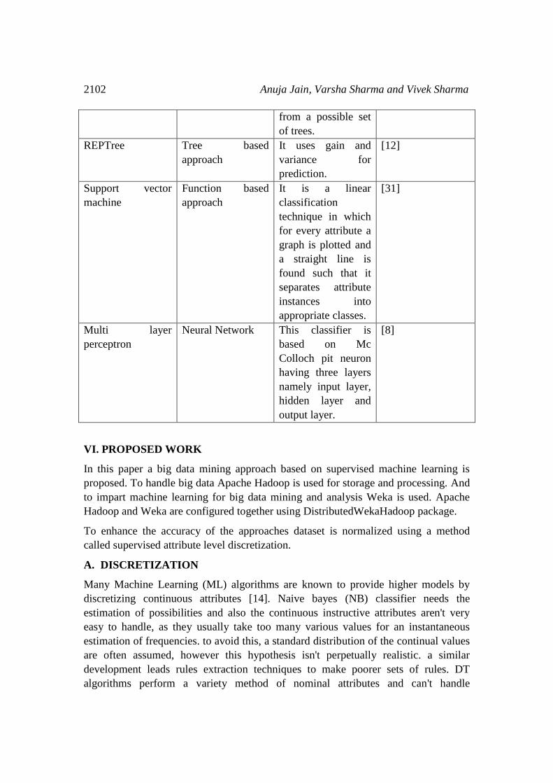
2102 Anuja Jain, Varsha Sharma and Vivek Sharma
from a possible set
of trees.
REPTree Tree based
approach
It uses gain and
variance for
prediction.
[12]
Support vector
machine
Function based
approach
It is a linear
classification
technique in which
for every attribute a
graph is plotted and
a straight line is
found such that it
separates attribute
instances into
appropriate classes.
[31]
Multi layer
perceptron
Neural Network This classifier is
based on Mc
Colloch pit neuron
having three layers
namely input layer,
hidden layer and
output layer.
[8]
VI. PROPOSED WORK
In this paper a big data mining approach based on supervised machine learning is
proposed. To handle big data Apache Hadoop is used for storage and processing. And
to impart machine learning for big data mining and analysis Weka is used. Apache
Hadoop and Weka are configured together using DistributedWekaHadoop package.
To enhance the accuracy of the approaches dataset is normalized using a method
called supervised attribute level discretization.
A. DISCRETIZATION
Many Machine Learning (ML) algorithms are known to provide higher models by
discretizing continuous attributes [14]. Naive bayes (NB) classifier needs the
estimation of possibilities and also the continuous instructive attributes aren't very
easy to handle, as they usually take too many various values for an instantaneous
estimation of frequencies. to avoid this, a standard distribution of the continual values
are often assumed, however this hypothesis isn't perpetually realistic. a similar
development leads rules extraction techniques to make poorer sets of rules. DT
algorithms perform a variety method of nominal attributes and can't handle
Big data mining using supervised machine learning approaches for Hadoop… 2103
continuous ones directly. As result, an outsized variety of ml and applied math
techniques will solely be applied to information sets composed entirely of nominal
variables. However, an awfully giant proportion of real information sets embrace
continuous variables: that's variables measured at the interval or magnitude relation
level. One answer to the present drawback is to partition numeric variables into
variety of sub-ranges and treat every such sub-range as a class. This method of
partitioning continuous variables into classes is sometimes termed discretization.
Sadly, the quantity of how to discretize a continual attribute is infinite. Discretization
could be a potential long bottleneck, since the variety of attainable discretization is
exponential within the number of interval threshold candidates at intervals the domain
[14]. The goal of discretization is to seek out a collection of cut points to partition the
range into a little variety of intervals that have sensible category coherence, that is
sometimes measured by an analysis operate. Additionally to the maximization of
reciprocality between category labels and attribute values, a perfect discretization
technique ought to have a secondary goal to reduce the quantity of intervals while not
important loss of class attribute mutual dependence. Discretization is sometimes
performed before the learning method and it are often broken into 2 tasks. The
primary task is to seek out the quantity of separate intervals. solely many
discretization algorithms perform this; usually, the user should specify the quantity of
intervals or give a heuristic. The second task is to seek out the width, or the
boundaries, of the intervals given the vary of values of a continual attribute. Usually,
in discretization method, once sorting information in ascending or drizzling order with
relation to the variable to be discretized, landmarks should be chosen among the
complete dataset. In general, the algorithmic rule for selecting landmarks are often
either topdown, that starts with an empty list of landmarks and splits intervals, or
bottom-up, that starts with the entire list of all the values as landmarks and merges
intervals. In each cases there's a stopping criterion, that specifies once to prevent the
discretization method. Researchers within the ml community have introduced several
discretization algorithms. Most of those algorithms perform an repetitive greedy
heuristic search within the space of candidate discretizations, exploitation differing
kinds of rating functions for evaluating a discretization. A recent outline of assorted
varieties of discretization algorithms are usually found in [28].
The term “cut-point” refers to a true value inside the range of continuous values that
divides the range into 2 intervals, one interval is a smaller amount than or equal to the
cutpoint and therefore the alternative interval is bigger than the cut-point. for instance,
an eternal interval [a, b] is divided into [a, c] and (c, b], wherever the worth c may be
a cut-point. Cut-point is additionally called split-point. The term “arity” within the
discretization context suggests that the amount of intervals or partitions. Before
discretization of an eternal feature, arity may be set to k—the range of partitions
within the continuous options. the most range of cut-points is k − 1. Discretization
method reduces the arity however there's a trade-off between arity and its impact on
2104 Anuja Jain, Varsha Sharma and Vivek Sharma
the accuracy. A typical discretization method loosely consists of 4 steps: (1) sorting
the continual values of the feature to be discretized, (2) evaluating a cut-point for
ripping or adjacent intervals for merging, (3) according to some criterion, ripping or
merging intervals of continuous value, and (4) finally stopping at some purpose. once
sorting, following step within the discretization method is to seek out the simplest
“cut-point” to separate a spread of continuous values or the simplest try of adjacent
intervals to merge. One typical analysis perform is to see the correlation of a split or a
merge with the category label. There ar various analysis functions found within the
literature like entropy measures and statistical measures (more details within the
following sections). A stopping criterion specifies once to prevent the discretization
method. it's typically ruled by a trade-off between lower arity with a far better
understanding however less accuracy and a higher arity with a poorer understanding
however higher accuracy. the amount of inconsistencies (inconsistency is outlined
later) caused by discretization—it shouldn't be abundant more than the amount of
inconsistencies of the first data before discretization. 2 instances are thought of
inconsistent if they're identical in their attribute values aside from their category
labels. Generally, the discretization ways may be classified as: (1) supervised or
unsupervised, (2) direct or progressive, (3) world or native, (4) static or dynamic, (5)
Top down or bottom-up. We have a tendency to distinct these classes within the
following section.
Feature generation is a three-step process: the first step is a pre-processing stage in
which the speech utterance has to be normalized and eventually noise-filtered or
smoothed. The second and third step correspond to the extraction of local and global
features, as can be seen in Figure 4.5. Features can indeed be different in nature,
depending on whether they capture local or global information. A speech utterance is
typically segmented into small blocks in which local computations are performed (ex:
energy, pitch of the window). Global features refer to all the computations performed
with local features; they use information from the whole utterance, whereas local
features are calculated for each block independently. The easiest ones are statistical
overall values such as mean, maximum, minimum, median, variance, range or inter
quartile range. More complex features include some in-between operations like the
following:
– curve simplification in linear segments like slopes or constant levels (ex:
stylization process of the pitch, macroscopic variations of the energy, etc...)
– combination of multiple local features (for example, mean energy of the
voiced segments)
– histogram derivation (for musical features)
Feature extraction is generally considered as a process of mapping the original
features (measurements) into more effective features. If the mapping is linear, the
Big data mining using supervised machine learning approaches for Hadoop… 2105
mapping function is well defined and the task is simply to find the coefficients of a
linear function so as to maximize or minimize a criterion. To determine these
mapping coefficients, we can use the linear algebra techniques for simple criteria and
we can apply optimization techniques for complex criteria. Unfortunately, in many
applications of pattern recognition, there are salient features which are non-linear
mappings of original measurements. Since there is no general theory to generate such
nonlinear functions systematically and find the optimum one, extraction of features
becomes problem-specific. In large multi-dimensional data sets, it is usually
advantageous to discover some structure from the data. Thus we assume that the data
are governed by a certain number of underlying parameters (features). The minimum
number of features required to account for the observed properties of the data is called
intrinsic dimensionality of the data set.
Principal component analysis (PCA) is a statistical procedure that uses an orthogonal
transformation to convert a set of observations of possibly correlated variables into a
set of values of linearly uncorrelated variables called principal components. The
number of principal components is less than or equal to the number of original
variables. This transformation is defined in such a way that the first principal
component has the largest possible variance (that is, accounts for as much of the
variability in the data as possible), and each succeeding component in turn has the
highest variance possible under the constraint that it is orthogonal to the preceding
components. The resulting vectors are an uncorrelated orthogonal basis set. The
principal components are orthogonal because they are the eigenvectors of the
covariance matrix, which is symmetric. PCA is sensitive to the relative scaling of the
original variables.
STEP OF HADOOP WEKA CONNECTIVITY FOR BIG DATA MINING
Step 1: Start Hadoop daemons ,the Apache Hadoop startup daemons.
The daemons that are running on standalone cluster. It shows NameNode, DataNode,
ResourceManager and NodeManager.
Step 2: Start Weka
A terminal in which command to start Weka jar is illustrated along with the Weka
startup GUI.
Step 3: Weka package manager for Hadoop connectivity
The Weka package manager to install Weka Hadoop distribution for Weka Hadoop
connectivity.
Step 4: Weka Knowledge flow Hadoop machine learning execution.
A. Putting data on HDFS from local file system.
2106 Anuja Jain, Varsha Sharma and Vivek Sharma
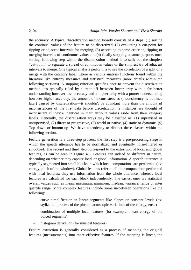
The Knowledge flow from Weka to load data from ARFF loader to HDFS saver.
The figure below shows the Apache Hadoop and Weka connectivity using Knowledge
flow in Weka.
Figure 1. Screenshot showing HDFS loader properties
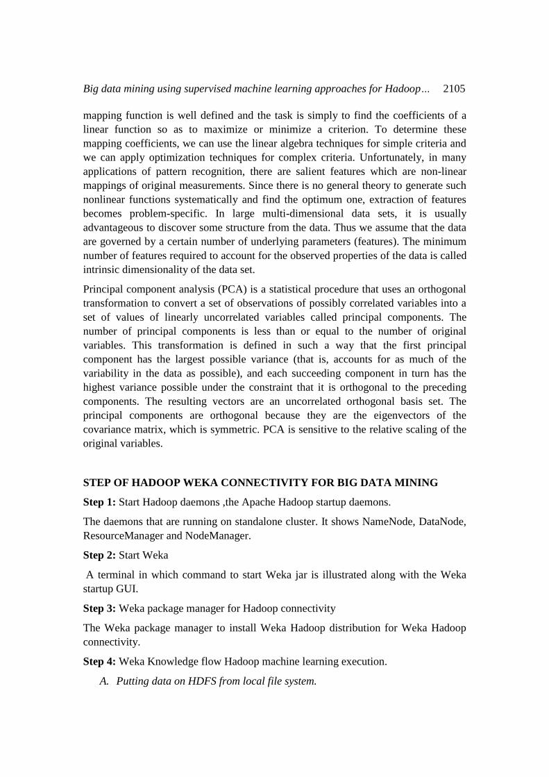
Figure shows the complete Knowledge flow to load the data from HDFS and class
assigner to pick the class from dataset and appropriate classifier which is Naïve Bayes
here and Text Viewer to view the results of classification.
Figure 2. Screenshot showing data processing
IV. RESULTS
A tool that is employed for each data processing and Machine Learning is weka. it was
1st enforced by The University of Waikato, New zealand, in 1997 [4]. It's a group of a
massive range of Machine Learning and data processing algorithms. One drawback of
this software package is that it supports data files solely written in ARFF (attribute
relation file format) and CSV (comma separated values) format. Initially, it absolutely
was written in C however later on it had been rewritten in JAVA language. It contains
of a graphical user interface interface for interaction with the data files. It possesses
forty nine knowledge pre-processing tools, fifteen attribute evaluators, seventy six
Big data mining using supervised machine learning approaches for Hadoop… 2107
classification algorithms and ten search algorithms for the aim of feature selection. It
contains of 3 differing types of graphical user interfaces (GUI’s):- “The Explorer”,
“The Experimenter”, and “The knowledge Flow”. Weka provides the chance for the
development of any new Machine Learning algorithmic rule. It contains visualization
tools and a collection of panels to execute the specified tasks.
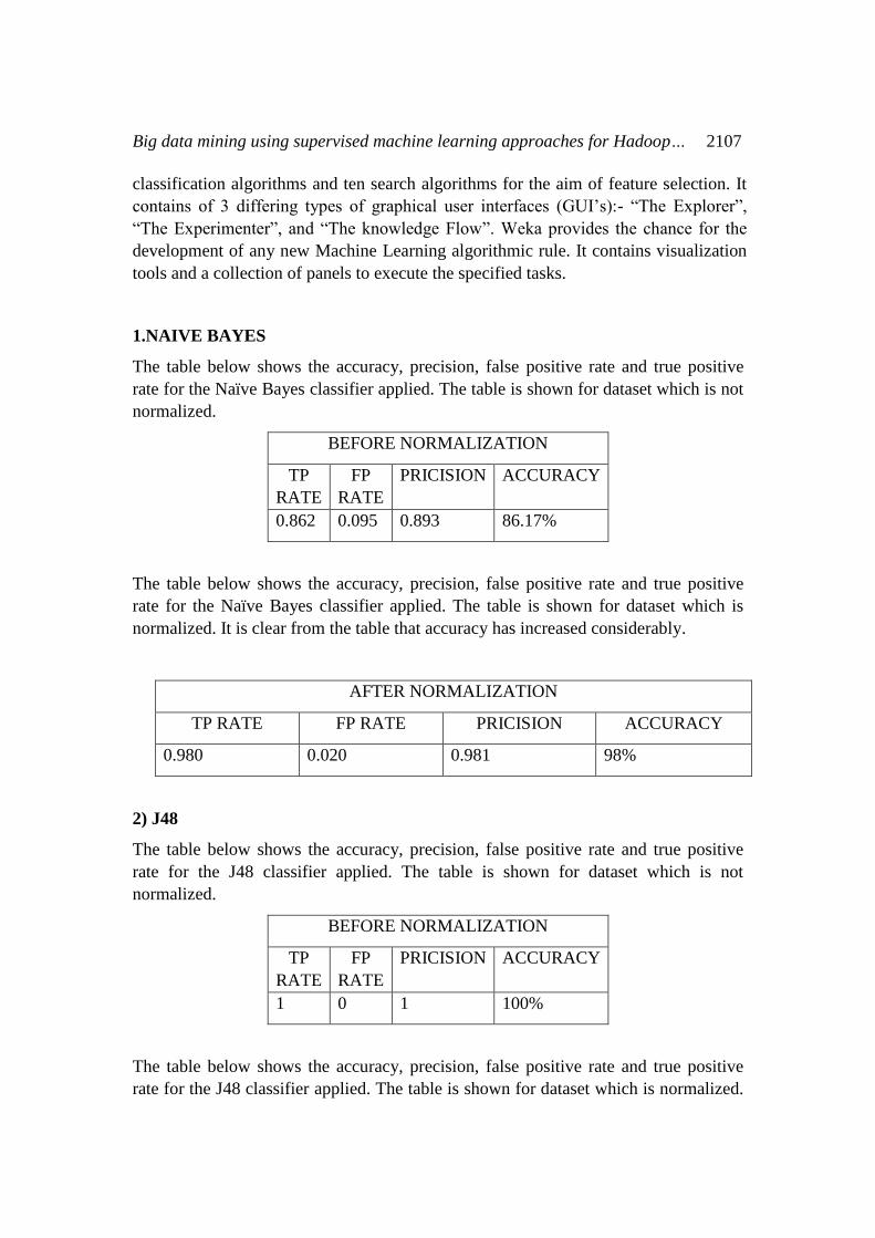
1.NAIVE BAYES
The table below shows the accuracy, precision, false positive rate and true positive
rate for the Naïve Bayes classifier applied. The table is shown for dataset which is not
normalized.
BEFORE NORMALIZATION
TP
RATE
FP
RATE
PRICISION ACCURACY
0.862 0.095 0.893 86.17%
The table below shows the accuracy, precision, false positive rate and true positive
rate for the Naïve Bayes classifier applied. The table is shown for dataset which is
normalized. It is clear from the table that accuracy has increased considerably.
AFTER NORMALIZATION
TP RATE FP RATE PRICISION ACCURACY
0.980 0.020 0.981 98%
2) J48
The table below shows the accuracy, precision, false positive rate and true positive
rate for the J48 classifier applied. The table is shown for dataset which is not
normalized.
BEFORE NORMALIZATION
TP
RATE
FP
RATE
PRICISION ACCURACY
1 0 1 100%
The table below shows the accuracy, precision, false positive rate and true positive
rate for the J48 classifier applied. The table is shown for dataset which is normalized.
2108 Anuja Jain, Varsha Sharma and Vivek Sharma
It is clear from the table that accuracy has increased considerably.
AFTER NORMALIZATION
TP RATE FP RATE PRICISION ACCURACY
1 0 1 100%
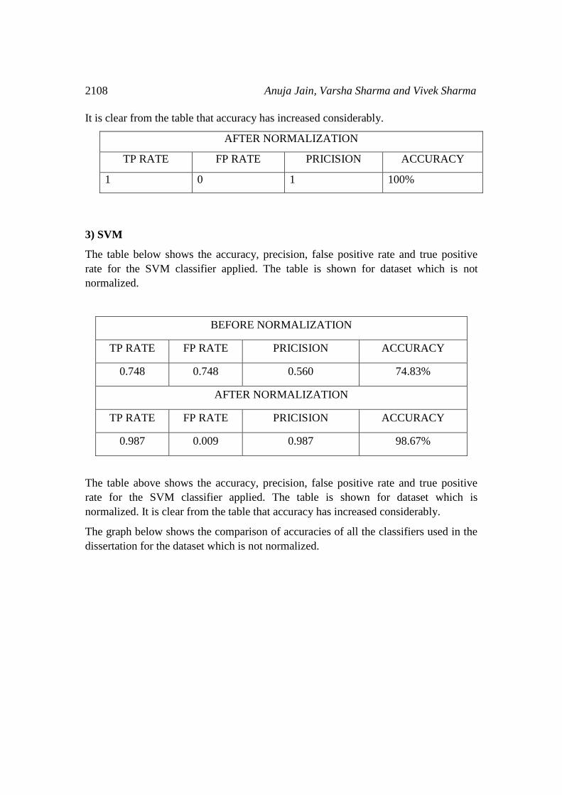
3) SVM
The table below shows the accuracy, precision, false positive rate and true positive
rate for the SVM classifier applied. The table is shown for dataset which is not
normalized.
BEFORE NORMALIZATION
TP RATE FP RATE PRICISION ACCURACY
0.748 0.748 0.560 74.83%
AFTER NORMALIZATION
TP RATE FP RATE PRICISION ACCURACY
0.987 0.009 0.987 98.67%
The table above shows the accuracy, precision, false positive rate and true positive
rate for the SVM classifier applied. The table is shown for dataset which is
normalized. It is clear from the table that accuracy has increased considerably.
The graph below shows the comparison of accuracies of all the classifiers used in the
dissertation for the dataset which is not normalized.
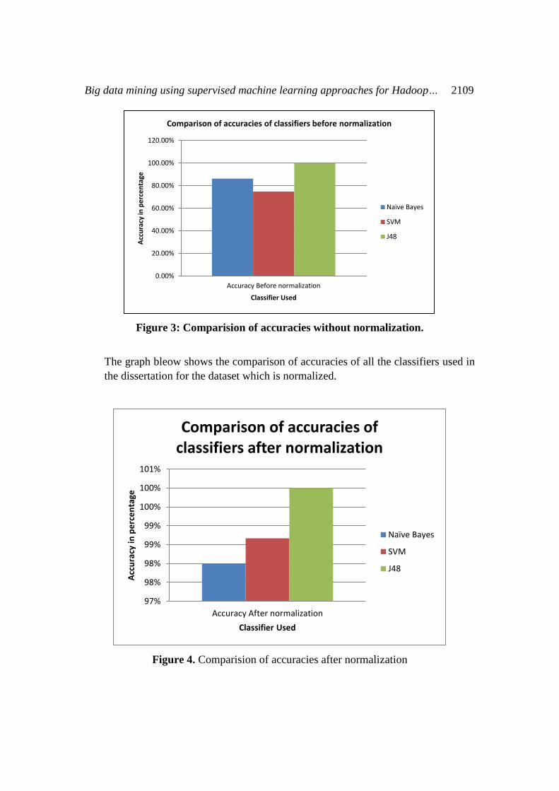
Big data mining using supervised machine learning approaches for Hadoop… 2109
Figure 3: Comparision of accuracies without normalization.
The graph bleow shows the comparison of accuracies of all the classifiers used in
the dissertation for the dataset which is normalized.
Figure 4. Comparision of accuracies after normalization
0.00%
20.00%
40.00%
60.00%
80.00%
100.00%
120.00%
Accuracy Before normalization
Acc
ura
cy in
pe
rce
nta
ge
Classifier Used
Comparison of accuracies of classifiers before normalization
Naïve Bayes
SVM
J48
97%
98%
98%
99%
99%
100%
100%
101%
Accuracy After normalization
Acc
ura
cy in
pe
rce
nta
ge
Classifier Used
Comparison of accuracies of classifiers after normalization
Naïve Bayes
SVM
J48

2110 Anuja Jain, Varsha Sharma and Vivek Sharma
V. CONCLUSION
In this era of data analytics, machine learning has emerged as a vital domain of
research. For classification and clustering of datasets different machine learning
techniques have been Machine learning algorithms can be broadly classified as
supervised and unsupervised approaches. In this dissertation supervised machine
learning techniques which include Naïve Bayes, Support vector machine and J48 have
been studied. But the objective of research is to increase the accuracy of classification
for the raw datasets. Here normalization has been applied on the raw dataset and it is
found that accuracy has been improved after supervised discretization of dataset.
In future the proposed scheme can be tested for other datasets also. And normalization
and feature selection approaches can be studied and suitable can be applied.
REFERENCES
[1] S. Amartya, K.D. Kundan, Application of Data mining Techniques in
Bioinformatics, B.Tech Computer Science Engineering thesis, National
Institute of Technology, (Deemed University), Rourkela, 2007.
[2] F. Bounch, F. Giannotti, C. Gozzi, G. Manco, M. Nanni, D. Pedreschi, C.
Renso, S. Ruggier, Web log data warehourseing and mining for intelligent
web caching, J. Data Knowledge Eng. 36 (2001) 165–189, PH:S0169-
023x(01)00038-6.
[3] L.D. Catledge, J. Pitkow, Characterizing browsing strategies in the world wide
web, J. Comput. Networks ISDN Syst. 27 (6) (1995) 1065–1073, doi:
101016/0169-7552(95)00043-7.
[4] R. Cooley, B. Mobasher, J. Srivastava, Data preparation for mining World
Wide Web browsing patterns, J. Knowledge Inform. Syst. 1 (1) (1999) 1–27.
[5] R. Cooley, P.N. Tan, J. Srivastava J, Discovery of Interesting Usage Patterns
from Web Data, International Workshop on Web Usage Analysis and User
Profiling, ISBN 3-540-67818-2, 2000, p. 163–182.
[6] A. Dario, B. Eleno, B. Giulia, C. Tania, C. Silvia, M. Naeem, Analysis of
diabetic patients through their examination history, J. Expert Syst. Appl. 40
(2013) 4672–4678.
[7] H. David, M. Heikki, S. Padhraic, Principles of Data Mining, The MIT press,
Cambridge. Massachusetts, London, England, 2001, p. 2–20.
[8] F.N. David, Data mining of social networks represented as graphs, J. Comput.
Sci. Rev. 7 (2013) (2012) 1– 34,
http://dx.doi.org/10.1016/j.cosrev.2012.12.001.
Big data mining using supervised machine learning approaches for Hadoop… 2111
[9] M.F. Federico, L.L. Pier, Mining interesting knowledge from weblog: a
survey, J. Data Knowledge Eng. 53 (2005) (2005) 225–241,
http://dx.doi.org/10.1016/j.datak.2004.08.001.
[10] C.N. Godswill, A Comprehensive Analysis of Predictive Data Mining
Techniques, M.Sc. Thesis, The University of Tennessee, Knoxville, 2006.
[11] L. Habin, K. Vlado, Combining mining of web server logs and web content
for classifying users’ navigation pattern and predicting users future request, J.
Data Knowledge Eng. 61 (2007) (2006) 304–330, http://
dx.doi.org/10.1016/j.datak.2006.06.001.
[12] M.K. James, R.G. Michael, A.G. James, A fuzzy K-Nearest Neighbor
Algorithm. IEEE Transactions on System Man and Cybernetics, vol. SMC-15
No4.[0018-9472/85/0700-0580$01.00], 1985.
[13] H. Jiawei, K. Micheline, Data mining concept and Techniques, second ed.,
Morgan Kaufmann Publishers, Elsevier inc., USA San Francisco, CA 94111,
2006, p. 285–350.
[14] E.P. Leif, K-Nearest Neighbor. Scholarpedia 4(2):1883. Downloaded 27-04-
2014,@ www.google.com, 2009.
[15] C. Luca, G. Paolo, Improving classification models with taxonomy
information, J. Data Knowledge Eng. 86 (2013) (2013) 85–101,
http://dx.doi.org/10.1016/j. datak.2013.01.005.
[16] T. Luigi, S. Giacomo, Mining frequent item sets in data streams within a time
horizon, J. Data Knowledge Eng. 89 (2014) 21–37,
http://dx.doi.org/10.1016/j.datak.2013.10.002.
[17] Mathworks Incorporation., MATLAB R2011b (7.13.0.564), Licence Number:
161052, USA, Mathworks Incorporation, 1984–2011.
[18] M. Michal, K. Jozef, S. Peter, Data preprocessing evaluation for web log
mining: reconstruction of activities of a web visitor, J. Proc. Comput. Sci. 1
(2012) (2012) 2273–2280.
[19] K. Mi-Yeon, H.L. Dong, Data-mining based SQL injection attack detection
using internal query trees, J. Expert Syst. Appl. 41 (2014) (2014) 5416–5430,
dx.doi.org/10.1016/j.eswa.2014.02.041.
[20] MySQL Corporation, MySQL Database Management System Software. USA
MySQL/Oracle Corporation, 2008.

2112 Anuja Jain, Varsha Sharma and Vivek Sharma