Findings of the Association for Computational Linguistics: ACL-IJCNLP 2021, pages 4640–4651August 1–6, 2021. ©2021 Association for Computational Linguistics

4640

Semi-Supervised Data Programming with Subset Selection

Ayush Maheshwari 1, Oishik Chatterjee 1, Krishnateja Killamsetty 2,Ganesh Ramakrishnan 1 , Rishabh Iyer 2

1Department of CSE, IIT Bombay, India2 The University of Texas at Dallas

{ayusham, oishik, ganesh}@cse.iitb.ac.in{krishnateja.killamsetty, rishabh.iyer}@utdallas.edu

Abstract

The paradigm of data programming, whichuses weak supervision in the form ofrules/labelling functions, and semi-supervisedlearning, which augments small amounts oflabelled data with a large unlabelled dataset,have shown great promise in several text classi-fication scenarios. In this work, we argue thatby not using any labelled data, data program-ming based approaches can yield sub-optimalperformances, particularly when the labellingfunctions are noisy. The first contribution ofthis work is an introduction of a framework,SPEAR which is a semi-supervised data pro-gramming paradigm that learns a joint modelthat effectively uses the rules/labelling func-tions along with semi-supervised loss func-tions on the feature space. Next, we also studySPEAR-SS which additionally does subset se-lection on top of the joint semi-superviseddata programming objective and selects a setof examples that can be used as the labelledset by SPEAR. The goal of SPEAR-SS isto ensure that the labelled data can comple-ment the labelling functions, thereby benefit-ing from both data-programming as well as ap-propriately selected data for human labelling.We demonstrate that by effectively combiningsemi-supervision, data-programming, and sub-set selection paradigms, we significantly out-perform the current state-of-the-art on sevenpublicly available datasets. 1

1 Introduction

Modern machine learning techniques rely on largeamounts of labelled training data for text clas-sification tasks such as spam detection, (movie)genre classification, sequence labelling, etc. Super-vised learning approaches have utilised such largeamounts of labelled data and, this has resulted in

1The source code is available athttps://github.com/ayushbits/Semi-Supervised-LFs-Subset-Selection

huge successes in the last decade. However, theacquisition of labelled data, in most cases, entailsa painstaking process requiring months of humaneffort. Several techniques such as active learning,distant supervision, crowd-consensus learning, andsemi-supervised learning have been proposed toreduce the annotation cost (Settles et al., 2008).However, clean annotated labels continue to be crit-ical for reliable results (Bach et al., 2019; Goh et al.,2018).

Recently, Ratner et al. (2016) proposed aparadigm on data-programming in which severalLabelling Functions (LF) written by humans areused to weakly associate labels with the instances.In data programming, users encode the weak su-pervision in the form of labelling functions. Onthe other hand, traditional semi-supervised learningmethods combine a small amount of labelled datawith large unlabelled data (Kingma et al., 2014).In this paper, we leverage semi-supervision in thefeature space for more effective data programmingusing labelling functions.

1.1 Motivating Example

We illustrate the LFs on one of the seven taskson which we experiment with, viz., identifyingspam/no-spam comments in the YouTube reviews.For some applications, writing LFs is often as sim-ple as using keyword lookups or a regex expression.In this specific case, the users construct heuristicpatterns as LFs for classifying spam/not-spam com-ments. Each LF takes a comment as an input andprovides a binary label as the output; +1 indicatesthat the comment is spam, -1 indicates that thecomment is not spam, and 0 indicates that the LF isunable to assert anything for the comment (referredto as an abstain). Table 1 presents a few exampleLFs for spam and non-spam classification.

In isolation, a particular LF may neither be al-ways correct nor complete. Furthermore, the LFs

4641

Id DescriptionLF1 If http or https in comment text, then return +1 otherwise

ABSTAIN (return 0)LF2 If length of comment is less than 5 words, then return -1 other-

wise ABSTAIN (return 0).(Non spam comments are often short)LF3 If comment contains my channel or my video, then return

+1 otherwise ABSTAIN (return 0).

Table 1: Three LFs based on keyword lookups or regexexpression for the YouTube spam classification task

may also produce conflicting labels. In the past,generative models such as Snorkel (Ratner et al.,2016) and CAGE (Chatterjee et al., 2020) havebeen proposed for consensus on the noisy and con-flicting labels assigned by the discrete LFs to deter-mine the probability of the correct labels. Labelsthus obtained could be used for training any super-vised model/classifier and evaluated on a test set.We will next highlight a challenge in doing dataprogramming using only LFs that we attempt to ad-dress. For each of the following sentences S1 . . . S6that can constitute an observed set of training in-stances, we state the value of the true label (±1).While the candidates in S1 and S4 are instances ofa spam comment, the ones in S2 and S3 are not. Infact, these examples constitute one of the canonicalcases that we discovered during the analysis of ourapproach in Section 4.4.1. 〈S1,+1〉: Please help me go to collegeguys! Thanks from the bottom of my heart.https://www.indiegogo.com/projects/

2. 〈S2,−1〉: I love this song3. 〈S3,−1〉: This song is very good... but thevideo makes no sense...4. 〈S4,+1〉: https://www.facebook.com/teeLaLaLa

Further, let us say we have a completely unseenset of test instances, S5 and S6, whose labels wewould also like to predict effectively:5. 〈S5,−1〉: This song is prehistoric6. 〈S6,+1〉: Watch Maroon 5’s latest ...www.youtube.com/watch?v=TQ046FuAu00

In Table 2, we present the outputs of the LFsas well as some n-gram features F1 (‘.com’) andF2 (‘This song’) on the observed training exam-ples S1, S2, S3 and S4 as well as on the unseentest examples S5 and S6. For S1, the correct con-sensus can easily be performed to output the truelabel +1, since LF1 (designed for class +1) getstriggered, whereas LF2 (designed for class -1) isnot triggered. Similarly, for S2, LF2 gets triggeredwhereas LF1 is not, making it possible to easilyperform the correct consensus. Hence, we havetreated S1 and S2 as unlabelled, indicating that we

Training data LF outputs Featuresid Label LF1(+1) LF2(-1) F1 F2S1 +1 1 0 1 0S2 -1 0 1 0 1S3 -1 0 0 0 1S4 +1 1 1 1 0

Test dataS5 -1 0 1 0 1S6 +1 0 0 1 0

Table 2: Example illustrating the insufficiency of usingdata programming using only LFs.

could learn a model based on LFs alone withoutsupervision if all we observed were these two ex-amples and the outputs of LF1 and LF2. However,the correct consensus on S3 and S4 is challengingsince both LF1 and LF2 either fire or do not. Whilethe (n-gram based) features F1 and F2 appear to beinformative and could potentially complement LF1and LF2, we can easily see that correlating featurevalues with LF outputs is tricky in a completelyunsupervised setup. To address this issue, we askthe following questions:(A) What if we are provided access to the true la-bels of a small subset of instances - in this case,only S3 and S4? Could the (i) correlation of fea-tures values (eg. F1 and F2) with labels (eg. +1and -1 respectively), modelled via a small set oflabelled instances (eg. S3 and S4), in conjunctionwith (ii) the correlation of feature values (eg. F1and F2) with LFs (eg. LF1 and LF2) modelled viaa potentially larger set of unlabelled instances (eg.S1, S2), help improved prediction of labels for hith-erto unseen test instances S5 and S6?(B) Can we precisely determine the subset of theunlabelled data that, when labelling would helpus train a model (in conjunction with the labellingfunctions) that is most effective on the test set? Inother words, instead of randomly choosing the la-belled dataset for doing semi-supervised learning(part A), can we intelligently select the labelledsubset? In the above example, choosing the la-belled set as S3, S4 would be much more usefulthan choosing the labelled set as S1, S2.

As a solution to (A), in Section 3.3, we presenta new formulation, SPEAR, in which the parame-ters over features and LFs are jointly trained in asemi-supervised manner. SPEAR expands as Semi-suPervisEd dAta pRogramming. As for (B), wepresent a subset selection recipe, SPEAR-SS (in

4642

Section 3.4), that recommends the sub-set of thedata (e.g. S3 and S4), which, after labelling, wouldmost benefit the joint learning framework.

1.2 Our Contributions

We summarise our main contributions as follows:To address (A), we present SPEAR (c.f., Sec-tion 3.3), which is a novel paradigm for jointlylearning the parameters over features and labellingfunctions in a semi-supervised manner. We jointlylearn a parameterized graphical model and a clas-sifier model to learn our overall objective. To ad-dress (B), we present SPEAR-SS (c.f., Section 3.4),which is a subset selection approach to select the setof examples which can be used as the labelled setby SPEAR. We show, in particular, that through aprincipled data selection approach, we can achievesignificantly higher accuracies than just randomlyselecting the seed labelled set for semi-supervisedlearning with labelling functions. Moreover, wealso show that the automatically selected subsetperforms comparably or even better than the hand-picked subset by humans in the work reported byAwasthi et al. (2020), further emphasising the ben-efit of subset selection for semi-supervised dataprogramming. Our framework is agnostic to theunderlying network architecture and can be appliedusing different underlying techniques without achange in the meta-approach. Finally, we evalu-ate our model on seven publicly available datasetsfrom domains such as spam detection, record clas-sification, and genre prediction and demonstratesignificant improvement over state-of-the-art tech-niques. We also draw insights from experiments insynthetic settings (presented in the appendix).

2 Related Work

Data Programming and Unsupervised Learn-ing: Snorkel (Ratner et al., 2016) has been pro-posed as a generative model to determine correctlabel probability using consensus on the noisyand conflicting labels assigned by the discreteLFs. Chatterjee et al. (2020) proposed a graphi-cal model, CAGE, that uses continuous-valued LFswith scores obtained using soft match techniquessuch as cosine similarity of word vectors, TF-IDFscore, distance among entity pairs, etc. Owing toits generative model, Snorkel is highly sensitive toinitialisation and hyper-parameters. On the otherhand, the CAGE model employs user-controlledquality guides that incorporate labeller intuition

into the model. However, these models completelydisregard feature information that could provide ad-ditional information to learn the (graphical) model.These models try to learn a combined model forthe labelling functions in an unsupervised manner.However, in practical scenarios, some labelled datais always available (or could be made availableby labelling a few instances); hence, a completelyunsupervised approach might not be the best solu-tion. In this work, we augment these data program-ming approaches by designing a semi-supervisedmodel that incorporates feature information andLFs to learn the parameters jointly. Hu et al. (2016)proposed a student-teacher model that transfersrule information by assigning linear weight to eachrule based on an agreement objective. The modelwe propose in this paper jointly learns parametersover features and rules in a semi-supervised man-ner rather than just weighing their outputs and cantherefore be more expressive.

Other works such as Jawanpuria et al. (2011);Dembczynski et al. (2008) discovers simple andconjuctive rules from input features and assignweight to each rules for better generalization.Nagesh et al. (2012) induces rules from query lan-guage to build NER extractor while Kulkarni et al.(2018) uses active learning to derive consensusamong labelers to label data.

Semi-Supervised Data Programming: The onlywork which, to our knowledge, combines ruleswith supervised learning in a joint framework isthe work by Awasthi et al. (2020). They leverageboth rules and labelled data by associating eachrule with exemplars of correct firings (i.e., instanti-ations) of that rule. Their joint training algorithmsdenoise over-generalized rules and train a classifi-cation model. Our approach differs from their workin two ways: a) we do not have information of ruleexemplars - thus our labelled examples need nothave any correspondence to any of the LFs (andmay instead complement the LFs as illustratedin Table 2) and b) we employ a semi-supervisedframework combined with graphical model for con-sensus amongst the LFs to train our model. We alsostudy how to automatically select the seed set oflabelled data, rather than having a human providethis seed set, as was done in (Awasthi et al., 2020).

Data Subset Selection: Finally, another approachthat has been gaining a lot of attention recentlyis data subset selection. The specific applicationof data subset selection depends on the goal at

4643

hand. Data subset selection techniques have beenused to reduce end to end training time (Mirza-soleiman et al., 2019; Kaushal et al., 2019; Killam-setty et al., 2021) and to select unlabelled points inan active learning manner to label (Wei et al., 2015;Sener and Savarese, 2017) or for topic summariza-tion (Bairi et al., 2015). In this paper, we presenta framework (SPEAR-SS) of data subset selectionfor selecting a subset of unlabelled examples forobtaining labels complementary to the labellingfunctions.

3 Methodology

3.1 Problem Description

Let X and Y ∈ {1...K} be the feature space andlabel space, respectively. We also have access to mlabelling functions (LF) λ1 to λm. As mentionedin Section 1.1, each LF λj is designed to recordsome class; let us denote2 by kj ∈ {1...K}, theclass associated with λj . The dataset consists of 2components, viz.,1. L = {(x1, y1, l1), (x2, y2, l2), . . . ,(xN , yN , lN )}, which denotes the labelled datasetand2. U = {(xN+1, lN+1), (xN+2, lN+2), . . . ,(xM , lM )}, which denotes the unlabelled datasetwherein xi ∈ X , yi ∈ Y .Here, the vector li = (li1, li2, . . . , lim) denotes thefirings of all the LFs on instance xi. Each lij canbe either 1 or 0. lij = 1 indicates that the LF λjhas fired on the instance i and 0 indicates it has not.All the labelling functions are discrete; hence, nocontinuous scores are associated with them.

3.2 Classification and Labelling FunctionModels

SPEAR has a feature-based classification modelfφ(x) which takes the features as input and predictsthe class label. Examples of fφ(x) we consider inthis paper are logistic regression and neural net-work models. The output of this model is P fφ (y|x),i.e., the probability of the classes given the inputfeatures. This model can be a simple classifica-tion model such as a logistic regression model or asimple neural network model.

We also use an LF-based graphical modelPθ(li, y) which, as specified in equation (1) foran example xi, is a generative model on the LF

2We use the association of LF λj with some class kj onlyin the quality guide component (QG) of the loss in eqn. 3

Notation Descriptionfφ The feature-based ModelP fφ The label probabilities as per the feature-based model fφPθ The label probabilities as per the LF-based Graphical Model

LCE Cross Entropy Loss: LCE(P fφ (y|x), y

)= − log

(P fφ (y = y|x)

)H Entropy function : H(P fφ (y|x)) = −

∑y

P fφ (y = y|x) logP fφ (y = y|x)

g Label Prediction from the LF-based graphical modelLLs Supervised negative log likelihoodLLu Unsupervised negative log likelihood summed over labelsKL KL Divergence between two probability modelsR Quality Guide based loss

Table 3: Summary of notation used.

outputs and class label y.

Pθ(li, y) =1

Zθ

m∏j=1

ψθ(lij , y) (1)

ψθ(lij , y) =

{exp(θjy) if lij 6= 0

1 otherwise.(2)

There are K parameters θj1, θj2...θjK for each LFλj , where K is the number of classes. The modelmakes the simple assumption that each LF λj inde-pendently acts on an instance xi to produce outputsli1, l1i...lim. The potentials ψθ invoked in equation(1) are defined in equation (2). Zθ is the normaliza-tion factor. We propose a joint learning algorithmwith semi-supervision to employ both features andLF predictions in an end-to-end manner.

3.3 Joint Learning in SPEARWe first specify the objective of SPEAR and there-after explain each of its components in greater de-tail:

minθ,φ

∑i∈L

LCE(P fφ (y|xi), yi

)+∑i∈U

H(P fφ (y|xi)

)+∑i∈U

LCE(P fφ (y|xi), g(li)

)+ LLs(θ|L)

+ LLu(θ|U) +∑i∈U∪L

KL(P fφ (y|xi), Pθ(y|li)

)+R(θ|{qj}) (3)

Before we proceed further, we refer the reader toTable 3 in which we summarise the notation builtso far as well as the notation that we will soon beintroducing.First Component (L1): The first compo-nent (L1) of the loss LCE

(P fφ (y|xi), yi

)=

− log(P fφ (y = yi|xi)

)is the standard cross-

entropy loss on the labelled dataset L for the modelP fφ .Second Component (L2): The second compo-nent L2 is the semi-supervised loss on the unla-belled data U . In our framework, we can use any

4644

unsupervised loss function. However, for this pa-per, we use the Entropy minimisation (Grandvaletand Bengio, 2005) approach. Thus, our secondcomponent H

(P fφ (y|xi)

)is the entropy of the

predictions on the unlabelled dataset. It acts as aform of semi-supervision by trying to increase theconfidence of the predictions made by the modelon the unlabelled dataset.Third Component (L3): The third componentLCE

(P fφ (y|xi), g(li)

)is the cross-entropy of the

classification model using the hypothesised labelsfrom CAGE (Chatterjee et al., 2020) on U . Giventhat li is the output vector of all labelling functionsfor any xi ∈ U , we specify the predicted label forxi using the LF-based graphical model Pθ(li, y)from eqn. (1) as: g(li) = argmaxyPθ(li, y).Fourth Component (L4): The fourth componentLLs(θ|L) is the (supervised) negative log likeli-hood loss on the labelled dataset L as per eqn. (3):

LLs(θ|L) = −N∑i=1

logPθ(li, yi)

Fifth Component (L5): The fifth componentLLu(θ|U) is the negative log likelihood loss forthe unlabelled dataset U as per eqn. (3). Since thetrue label information is not available, the proba-bilities need to be summed over y: LLu(θ|U) =

−M∑

i=N+1

log∑y∈Y

Pθ(li, y)

Sixth Component (L6): The sixth componentKL(P fφ (y|xi), Pθ(y|li)) is the Kullback-Leibler(KL) divergence between the predictions of boththe models, viz., feature-based model fφ and theLF-based graphical model Pθ summed over everyexample xi ∈ U ∪ L. Through this term, we tryand make the models agree in their predictions overthe union of the labelled and unlabelled datasets.Quality Guides (QG): As the last component inour objective, we use quality guides R(θ|{qj}) onLFs, which have been shown in (Chatterjee et al.,2020) to stabilise the unsupervised likelihood train-ing while using labelling functions. Let qj be thefraction of cases where λj correctly triggered, andlet qtj be the user’s belief on the fraction of exam-ples xi where yi and lij agree. If the user’s beliefswere not available, we consider the precision of theLFs on the validation set as the user’s beliefs. Ex-cept for the SMS dataset, we take the precision ofthe LFs on the validation set as the quality guides.If Pθ(yi = kj |lij = 1) is the model-based preci-sion over the LFs, the quality guide based loss canbe expressed as R(θ|{qtj}) =

∑j q

tj logPθ(yi =

kj |lij = 1)+(1−qtj) log(1−Pθ(yi = kj |lij = 1)).Throughout the paper, we consider QG always inconjunction with Loss L5.

In summary, the first three components (L1, L2and L3) invoke losses on the supervised modelfφ. While L1 compares the output fφ against theground truth in the labelled set L, L2 and L3 op-erate on the unlabelled data U by minimizing theentropy of fφ (L2) and by calibrating the fφ outputagainst the noisy predictions g(li) of the graphicalmodel Pθ(li, y) for each xi ∈ U (L3). The nexttwo components L4 and L5 focus on maximizingthe likelihood of the parameters θ of Pθ(li, y) overlabelled xi ∈ L and unlabelled xi ∈ U datasetsrespectively. Finally, in L6, we compare the prob-abilistic outputs from the supervised model fφagainst those from the graphical model Pθ(l, y)through a KL divergence based loss. We use theADAM (stochastic gradient descent) optimizer totrain the non-convex loss objective.

Previous data programming approaches (Bachet al., 2019; Chatterjee et al., 2020) adopt a cas-caded approach in which they first optimise a vari-ant of L5 to learn the θ parameters associated withthe LFs and thereafter use the noisily generatedlabels using g(l) to learn the supervised model fφusing a variant of L3. In contrast, our approachlearns the LF’s θ parameters and the model’s φparameters jointly in the context of the unlabelleddata U .

We present synthetic experiments to illustrate theeffect of SPEAR for data programming and semi-supervision in a controlled setting in which (i) theoverlap between classes in the data is controlledand (ii) the labelling functions are accurate. Thedetails of the synthetic experiments are provided inthe appendix.

3.4 SPEAR-SS: Subset Selection with SPEAR

Suppose we are given an unlabelled data set U anda limited budget for data labelling because of thecosts involved in it. It is essential for us to choosethe data points that need to be labelled properly.We explore two strategies for selecting a subsetof data points from the unlabelled set. We thenobtain the labels for this subset, and run SPEAR onthe combination of this labelled and unlabelled set.The two approaches given are intended to maximisediversity of the selected subset in the feature space.We complement both the approaches with EntropyFiltering (also described below).

4645

Unsupervised Facility Location: In this ap-proach, given an unlabelled data-set U , we wantto select a subset S such that the selected subsethas maximum diversity with respect to the fea-tures. Inherently, we are trying to maximise theinformation gained by a machine learning modelwhen trained on the subset selected. The objec-tive function for unsupervised facility location isfunsup(S) =

∑i∈U maxj∈S σij where σij denotes

the similarity score (in the feature space X ) be-tween data instance xi in unlabelled set U and datainstance xj in selected subset data S. We employa lazy greedy strategy to select the subset. In con-junction with Entropy Filtering described below,wecall this technique Unsupervised Subset Selection.Supervised Facility Location: The objec-tive function for Supervised Facility Lo-cation (Wei et al., 2015) is fsup(S) =∑

y∈Y∑

i∈Uy maxj∈S∩Uy σij . Here we as-sume that Uy ⊆ U is the subset of data pointswith hypothesised label y. Simply put, Uy formsa partition of U based on the hypothesized labelsobtained by performing unsupervised learning withlabelling functions. In conjunction with EntropyFiltering, we call this technique Supervised SubsetSelection.Entropy Filtering: We also do a filtering basedon entropy. In particular, we sort the examplesbased on maximum entropy and select fB numberof data points3, where B is the data selection bud-get (which was set to the size of the labelled set|L| in all our experiments). On the filtered dataset,we perform the subset selection, using either thesupervised or unsupervised facility location as de-scribed above. Below, we describe the optimisationalgorithm for subset selection.Optimisation Algorithms and Submodularity:Both funsup(S) and fsup(S) are submodular func-tions. We select a subset S of the filtered unla-belled data, by maximising these functions undera cardinality budget k (i.e., a labelling budget).For cardinality constrained maximisation, a simplegreedy algorithm provides a near-optimal solution(Nemhauser et al., 1978). Starting with S0 = ∅,we sequentially update

St+1 = St ∪ argmaxj∈U\St

f(j|St) (4)

where f(j|S) = f(S ∪ j)− f(S) is the gain ofadding element j to set S. We iteratively executethe greedy step (4) until t = k and |St| = k. It

3In our experiments, we set f = 5

is easy to see that the complexity of the greedyalgorithm is O(nkTf ), where Tf is the complexityof evaluating the gain f(j|S) for the supervised andunsupervised facility location functions. We thensignificantly optimize this simple greedy algorithmvia a lazy greedy algorithm (Minoux, 1978) viamemoization and precompute statistics (Iyer andBilmes, 2019).

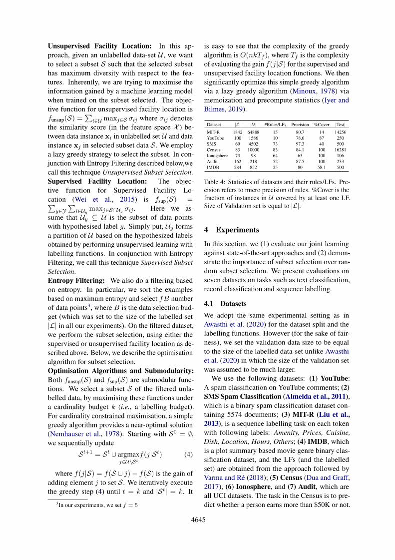
Dataset |L| |U| #Rules/LFs Precision %Cover |Test|MIT-R 1842 64888 15 80.7 14 14256YouTube 100 1586 10 78.6 87 250SMS 69 4502 73 97.3 40 500Census 83 10000 83 84.1 100 16281Ionosphere 73 98 64 65 100 106Audit 162 218 52 87.5 100 233IMDB 284 852 25 80 58.1 500

Table 4: Statistics of datasets and their rules/LFs. Pre-cision refers to micro precision of rules. %Cover is thefraction of instances in U covered by at least one LF.Size of Validation set is equal to |L|.

4 Experiments

In this section, we (1) evaluate our joint learningagainst state-of-the-art approaches and (2) demon-strate the importance of subset selection over ran-dom subset selection. We present evaluations onseven datasets on tasks such as text classification,record classification and sequence labelling.

4.1 DatasetsWe adopt the same experimental setting as inAwasthi et al. (2020) for the dataset split and thelabelling functions. However (for the sake of fair-ness), we set the validation data size to be equalto the size of the labelled data-set unlike Awasthiet al. (2020) in which the size of the validation setwas assumed to be much larger.

We use the following datasets: (1) YouTube:A spam classification on YouTube comments; (2)SMS Spam Classification (Almeida et al., 2011),which is a binary spam classification dataset con-taining 5574 documents; (3) MIT-R (Liu et al.,2013), is a sequence labelling task on each tokenwith following labels: Amenity, Prices, Cuisine,Dish, Location, Hours, Others; (4) IMDB, whichis a plot summary based movie genre binary clas-sification dataset, and the LFs (and the labelledset) are obtained from the approach followed byVarma and Re (2018); (5) Census (Dua and Graff,2017), (6) Ionosphere, and (7) Audit, which areall UCI datasets. The task in the Census is to pre-dict whether a person earns more than $50K or not.

4646

Ionosphere is radar binary classification task givena list of 32 features. The task in the Audit is toclassify suspicious firms based on the present andhistorical risk factors.

Statistics pertaining to these datasets are pre-sented in Table 4. Since we compare performancesagainst models that adopt different terminology, werefer to rules and labelling functions interchange-ably. For fairness, we restrict the size of the vali-dation set and keep it equal to the size |L| of thelabelled set. For all experiments involving com-parison with previous approaches, we used codeand hyperparameters from (Awasthi et al., 2020)but with our smaller-sized validation set. Note thatwe mostly outperform them even with their larger-sized validation set as can be seen in Table 5. Moredetails on training and validation set size are givenin the appendix.

4.2 Baselines

In Table 5, we compare SPEAR and SPEAR-SSagainst other following standard methods on sevendatasets.Only-L: We train the classifier Pθ(y|x) only onthe labelled data L using loss component L1. Asexplained earlier, following (Awasthi et al., 2020),we observe that a 2-layered neural network trainedwith the small amount of labelled data is capableof achieving competitive accuracy. We choose thismethod as a baseline and report gains over it.L + Umaj : We train the baseline classifierPθ(y|x) on the labelled data L along with Umajwhere labels on the U instances are obtained bymajority voting on the rules/LFs. The trainingloss is obtained by weighing instances labelledby rules as minθ

∑(xi,li)∈L− logPθ(li|xi) +

γ∑

(xi,yi)∈L− logPθ(yi|xi).Learning to Reweight (L2R) (Ren et al., 2018):This method trains the classifier by an online train-ing algorithm that assigns importance to examplesbased on the gradient direction.L+USnorkel (Ratner et al., 2016): Snorkel’s gen-erative model that models class probabilities basedon discrete LFs for consensus on the noisy and con-flicting labels.Posterior Regularization (PR) (Hu et al., 2016):This is a method for joint learning of a rule andfeature network in a teacher-student setup.Imply Loss (Awasthi et al., 2020): This approachuses additional information in the form of labelledrule exemplars and trains with denoised rule-label

loss. Since it uses information in addition to whatwe assume, Imply Loss can be considered as askyline for our proposed approaches.

4.3 Results with SPEAR

SPEAR uses the ‘best’ combination of the loss com-ponents L1, L2, L3, L4, L5, L6. To determinethe ‘best’ combination, we perform a grid searchover various combinations of losses using valida-tion accuracy/f1-score as the criteria for selectingthe most appropriate loss combination. Imply Lossuses a larger-sized validation set to tune their mod-els. In our experiments, we maintained a validationset size equal to the size of the labelled data. InTable 5, we observe that SPEAR performs signifi-cantly better than all other approaches on all butthe MIT-R data-set. Please note that all results arebased on the same hand-picked labelled data subsetas was chosen in prior work (Awasthi et al., 2020;Varma and Re, 2018), except for Audit and Iono-sphere. Even though we do not have rule-exemplarinformation in our model, SPEAR achieves bettergains than even ImplyLoss. Recall that the use ofImplyLoss can be viewed as a skyline approachowing to the additional exemplar information thatassociates labelling functions with specific labelledexamples. The slightly lower performance of the‘best’ SPEAR on the MIT-R data-set can be par-tially explained by the fact that there are no LFscorresponding to the ‘0’ class label, owing to whichour graphical model is not trained for all classes.However, as we will show in the next section, bysuitably determining a subset of the data-set thatcan be labelled (using the facility location represen-tation function), we achieve improved performanceeven on the MIT-R data-set (see Table 5). Also,note that in Table 5, we present results on two ver-sions of Audit, one in which both the train andtest set are balanced, and the other where the la-belled training set is imbalanced. In the imbalancedcase (where the number of positives are only 10%),we were unable to successfully run the ImplyLossand Posterior-Reg models (and hence the ‘-’), de-spite communication with the authors. We seethat SPEAR and similarly, SPEAR-SS (discussedbelow) significantly outperform the baselines by al-most 40% in the imbalanced case. In the balancedcase, the gains are similar to what we observe onthe other datasets.

4647

MethodsDatasets

YouTube[Accuracy]

SMS[F1]

MIT-R[F1]

IMDB[F1]

Census[Accuracy]

Ionosphere[F1]

Audit (Imb)[F1]

Audit (Bal)[F1]

Only-L (Handpicked) 90.7 (1.2) 90.0 (3.7) 74.1 (0.4) 72.2 (3.1) 78.3 (0.3) 92.7 (0.5) 24.7(2.6) 87.3 (0.9)

L+Umaj (Handpicked) +1.9 (1.1) -0.3 (1.4) +0.1(0.2) +1.2 (0.3) -0.9 (0.4) +0.4 (0.7) -4.8 (6) -1.4(4.2)

L2R (Ren et al., 2018) (Handpicked) -3.7 (5.1) +0.7 (2.9) -20.2(0.9) +4.5(0.2) +3.6(0.3) -18.8 (0.3) -1.2(3.2) -3.0(4.9)

L+USnorkel (Ratner et al., 2016) (Handpicked) +0.9 (2.6) +0.3 (4.5) -0.3(0.2) +0.6(1.8) +1.7 (0.2) -0.6 (0.5) -7.4(3.4) -0.6(4.2)

Posterior Reg (Hu et al., 2016) (Handpicked) -1.9(1.6) -3.3 (1.9) -0.2 (0.2) +1.1 (0.7) -1.9 (0) -0.1(0.7) - +0.1 (1.4)

ImplyLoss (Awasthi et al., 2020) (Handpicked) +0.4 (0.5) +0.9(0.9) 0.9(0.4) +4.3 (1.5) +3.4 (0.1) -3.9(2.4) - +0.5(1)

SPEAR (Handpicked) +3.7(0.5) +3.4(0.9) -0.8 (0.5) +4.9(0.3) +3.7 (0.3) +5.4 (0.3) +44 (0.9) +4.3 (0.9)

SPEAR-SS (Random Subset Selection) +3.5 +1.8 -2.9 +4.0 -5.2 +4.7 +41.7 +2.0SPEAR-SS (Unsupervised Subset Selection) +3.9 +1.9 +2.6 -0.6 +2.5 +4.8 +43.5 +3.3SPEAR-SS (Supervised Subset Selection) +4.2 +3.2 +2.9 +6.3 +2.5 +5.1 +44.5 +3.5

Table 5: Performance of SPEAR and SPEAR-SS for three subset selection schemes on seven data-sets. All numbersreported are gains over the baseline method (Only-L). All results are averaged over 5 runs. Numbers in brackets‘()’ represent standard deviation of the original score. Handpicked instances refers to instances selected from thedataset for designing LFs. These instances are taken directly from (Awasthi et al., 2020) to ensure fair comparison.

4.4 Results with SPEAR-SS

Recall that all results discussed so far (includingthose for SPEAR) on the Youtube, SMS, MIT-R,IMDB and Census datasets were based on thesame ‘hand-picked’ labelled data subset as in priorwork (Awasthi et al., 2020; Varma and Re, 2018).In the case of Audit and Ionosphere, the labelledsubset was randomly picked. In Table 5, we sum-marise the results obtained by employing super-vised and unsupervised subset selection schemesfor picking the labelled data-set and present com-parisons against results obtained using (i) ‘hand-picked’ labelled data-sets, and (ii) random selec-tion of the labelled set. In each case, the size ofthe subset is the same, which we set to be thesize of the hand-picked labelled set. Our data se-lection schemes are applied to the ‘best’ SPEAR

model obtained across various loss components.We observe that the best-performing model forthe supervised and unsupervised data selectiontends to outperform the best model based on ran-dom selection. Secondly, we observe that betweenthe supervised and unsupervised data selection ap-proaches, the supervised one tends to perform thebest, which means that using the hypothesised la-bels does help. Thirdly, we observe that YouTube,MIT-R, IMDB and Audit using the selected subsetoutperform prior work that employ hand pickeddata-set, whereas, in the case of SMS, Census andIonosphere, we come close. Finally, our approachis more stable than other approaches as the stan-dard deviation of SPEAR is low for 5 different runsacross all the datasets.

As an illustration, the examples such as S3and S4 referred to in Section 1.1 were preciselyobtained through supervised subset selection in

SPEAR-SS, to form part of the labelled dataset. Aspreviously observed in Table 2, S3 and S4 comple-ment (via n-grams features such as F1 and F2) theeffect of the labelling functions LF1 and LF2 onthe unlabelled examples such as S1 and S2, whenincluded in the labelled set. Further detailed resultswith subset selection, etc. can be found in the ap-pendix. In general, we observe that when the subsetof instances selected for labelling is complemen-tary to the labelling functions (as in our case), theperformance is higher than when the labelled exam-ples (exemplars) are inspired by labelling functionsthemselves as done in the work by Awasthi et al.(2020).

4.5 Significance Test

We employ the Wilcoxon signed-rank test(Wilcoxon, 1992) to determine whether there isa significant difference between SPEAR and ImplyLoss (current state-of-the-art). Our null hypothesisis that there is not significant difference betweenSPEAR and Imply loss. For n = 7 instances, we ob-serve that the one-tailed hypothesis is significant atp < .05, so we reject the null hypothesis. Clearly,SPEAR significantly outperforms Imply loss and,therefore, all previous baselines.

Similarly, we perform the significance test toassess the difference between SPEAR-SS and Im-ply Loss. As expected, the one-tailed hypothesisis significant at p < 0.05, which implies that ourSPEAR-SS approach significantly outperforms Im-ply Loss, and thus all other approaches.

5 Conclusion

We study how data programming can benefit fromlabelled data by learning a model (SPEAR) that

4648

Methods Datasets

YouTube[Accuracy]

SMS[F1]

MIT-R[F1]

Census[Accuracy]

ImplyLoss (Awasthi et al.,2020)

94.1 93.2 74.3 81.1

SPEAR (Handpicked) +0.3 +0.2 -0.9 +0.9SPEAR-SS (Supervised Sub-set Selection)

+0.8 0.0 +1.7 -0.3

Table 6: Comparison of SPEAR and SPEAR-SS againstImplyLoss on subset of datasets from Table 5 for whichImplyLoss used a much larger validation set than |L|.JL uses a validation set sizes equal to |L|.

jointly optimises the consensus obtained from la-belling functions in an unsupervised manner, alongwith semi-supervised loss functions designed inthe feature space. We empirically assess the per-formance of the different components of our jointloss function. As another contribution, we alsostudy some subset selection approaches to guidethe selection of the labelled subset of examples. Wepresent the performance of our models and presentinsights on both synthetic and real datasets. Whileoutperforming previous approaches, our approachis often better than an exemplar-based (skyline) ap-proach that uses the additional information of theassociation of rules with specific labelled exam-ples.

Acknowledgements

We thank anonymous reviewers for providing con-structive feedback. Ayush Maheshwari is sup-ported by a Fellowship from Ekal Foundation(www.ekal.org). We are also grateful to IBM Re-search, India (specifically the IBM AI Horizon Net-works - IIT Bombay initiative) for their supportand sponsorship.

References

Tiago A Almeida, Jose Marıa G Hidalgo, and AkeboYamakami. 2011. Contributions to the study of smsspam filtering: new collection and results. In Pro-ceedings of the 11th ACM symposium on Documentengineering, pages 259–262.

Abhijeet Awasthi, Sabyasachi Ghosh, Rasna Goyal,and Sunita Sarawagi. 2020. Learning from rulesgeneralizing labeled exemplars. In 8th InternationalConference on Learning Representations, ICLR2020, Addis Ababa, Ethiopia, April 26-30, 2020.OpenReview.net.

Stephen H Bach, Daniel Rodriguez, Yintao Liu, ChongLuo, Haidong Shao, Cassandra Xia, Souvik Sen,Alex Ratner, Braden Hancock, Houman Alborzi,

et al. 2019. Snorkel drybell: A case study in deploy-ing weak supervision at industrial scale. In Proceed-ings of the 2019 International Conference on Man-agement of Data, pages 362–375.

Ramakrishna Bairi, Rishabh Iyer, Ganesh Ramakrish-nan, and Jeff Bilmes. 2015. Summarization of multi-document topic hierarchies using submodular mix-tures. In Proceedings of the 53rd Annual Meet-ing of the Association for Computational Linguisticsand the 7th International Joint Conference on Natu-ral Language Processing (Volume 1: Long Papers),pages 553–563.

Oishik Chatterjee, Ganesh Ramakrishnan, and SunitaSarawagi. 2020. Robust data programming withprecision-guided labeling functions. In AAAI.

Krzysztof Dembczynski, Wojciech Kotłowski, and Ro-man Słowinski. 2008. Maximum likelihood rule en-sembles. In Proceedings of the 25th internationalconference on Machine learning, pages 224–231.

Dheeru Dua and Casey Graff. 2017. UCI machinelearning repository.

Garrett B Goh, Charles Siegel, Abhinav Vishnu, andNathan Hodas. 2018. Using rule-based labels forweak supervised learning: a chemnet for transfer-able chemical property prediction. In Proceedingsof the 24th ACM SIGKDD International Conferenceon Knowledge Discovery & Data Mining, pages302–310.

Yves Grandvalet and Yoshua Bengio. 2005. Semi-supervised learning by entropy minimization. InAdvances in neural information processing systems,pages 529–536.

Zhiting Hu, Xuezhe Ma, Zhengzhong Liu, Eduard H.Hovy, and Eric P. Xing. 2016. Harnessingdeep neural networks with logic rules. CoRR,abs/1603.06318.

Rishabh Iyer and Jeff Bilmes. 2019. A memoiza-tion framework for scaling submodular optimiza-tion to large scale problems. arXiv preprintarXiv:1902.10176.

Pratik Jawanpuria, Saketha N Jagarlapudi, and GaneshRamakrishnan. 2011. Efficient rule ensemble learn-ing using hierarchical kernels. In Proceedings of the28th International Conference on Machine Learning(ICML-11), pages 161–168.

Vishal Kaushal, Rishabh Iyer, Suraj Kothawade, RohanMahadev, Khoshrav Doctor, and Ganesh Ramakrish-nan. 2019. Learning from less data: A unified datasubset selection and active learning framework forcomputer vision. In 2019 IEEE Winter Conferenceon Applications of Computer Vision (WACV), pages1289–1299. IEEE.

Krishnateja Killamsetty, Durga Sivasubramanian,Ganesh Ramakrishnan, and Rishabh Iyer. 2021.Glister: Generalization based data subset selectionfor efficient and robust learning. In AAAI.

4649

Durk P Kingma, Shakir Mohamed, Danilo JimenezRezende, and Max Welling. 2014. Semi-supervisedlearning with deep generative models. In Advancesin neural information processing systems, pages3581–3589.

Ashish Kulkarni, Narasimha Raju Uppalapati, PankajSingh, and Ganesh Ramakrishnan. 2018. An interac-tive multi-label consensus labeling model for multi-ple labeler judgments. In Proceedings of the Thirty-Second AAAI Conference on Artificial Intelligence,(AAAI), 2018, pages 1479–1486. AAAI Press.

Jingjing Liu, Panupong Pasupat, Yining Wang, ScottCyphers, and Jim Glass. 2013. Query understandingenhanced by hierarchical parsing structures. In 2013IEEE Workshop on Automatic Speech Recognitionand Understanding, pages 72–77. IEEE.

Michel Minoux. 1978. Accelerated greedy algorithmsfor maximizing submodular set functions. In Opti-mization techniques, pages 234–243. Springer.

Baharan Mirzasoleiman, Jeff Bilmes, and JureLeskovec. 2019. Data sketching for faster train-ing of machine learning models. arXiv preprintarXiv:1906.01827.

Ajay Nagesh, Ganesh Ramakrishnan, Laura Chiti-cariu, Rajasekar Krishnamurthy, Ankush Dharkar,and Pushpak Bhattacharyya. 2012. Towards effi-cient named-entity rule induction for customizabil-ity. In Proceedings of the 2012 Joint Conferenceon Empirical Methods in Natural Language Process-ing and Computational Natural Language Learning,pages 128–138, Jeju Island, Korea. Association forComputational Linguistics.

George L Nemhauser, Laurence A Wolsey, and Mar-shall L Fisher. 1978. An analysis of approximationsfor maximizing submodular set functions—i. Math-ematical programming, 14(1):265–294.

Alexander J Ratner, Christopher M De Sa, Sen Wu,Daniel Selsam, and Christopher Re. 2016. Data pro-gramming: Creating large training sets, quickly. InAdvances in neural information processing systems,pages 3567–3575.

Mengye Ren, Wenyuan Zeng, Bin Yang, and RaquelUrtasun. 2018. Learning to reweight examples forrobust deep learning. In International Conferenceon Machine Learning, pages 4334–4343.

Ozan Sener and Silvio Savarese. 2017. Active learn-ing for convolutional neural networks: A core-setapproach. arXiv preprint arXiv:1708.00489.

Burr Settles, Mark Craven, and Lewis Friedland. 2008.Active learning with real annotation costs. In Pro-ceedings of the NIPS workshop on cost-sensitivelearning, pages 1–10. Vancouver, CA:.

Paroma Varma and Christopher Re. 2018. Snuba: Au-tomating weak supervision to label training data.Proc. VLDB Endow., 12(3):223–236.

Kai Wei, Rishabh Iyer, and Jeff Bilmes. 2015. Submod-ularity in data subset selection and active learning.In International Conference on Machine Learning,pages 1954–1963.

Frank Wilcoxon. 1992. Individual comparisons byranking methods. In Breakthroughs in statistics,pages 196–202. Springer.

A Illustration of SPEAR on a syntheticsetting

Through a synthetic example, we illustrate the ef-fectiveness of our formulation of combining semi-supervised learning with labelling functions (i.e.,combined Losses 1-6) to achieve superior perfor-mance. Consider a 3-class classification problemwith overlap in the feature space as depicted inFigure 1. The classes are A, B and C. Though weillustrate the synthetic setting in 2 dimensions, inreality, we performed similar experiments in threedimensions (and results were similar). We ran-

Figure 1: Synthetic data

domly pick 5 points from each class i ∈ {a, b, c},and corresponding to each such point (xi, yi) wecreate a labelling function based on its coordinates:

• LFa: Consider the point (xa, ya). The corre-sponding LF will be: if y ≥ ya return 1 (i.e.classify as class A) else return 0 (abstain).

• LFb: Similarly for (xb, yb) the LF will return1 if x ≤ xb and else will return 0.

• LFc: The LF corresponding to (xc, yc) willreturn 1 if x ≥ xc and else will return 0.

These seemingly 15 weak labelling functions (5for each class) actually aid in classification whenthe labelled example set is extremely small andthe classifier is unable to get a good estimate ofthe class boundaries. This can be observed in Ta-ble 7 wherein we report the F1 score on a heldout test dataset for models obtained by trainingon the different loss components. The results arereported in the case of three dimensions, whereineach circle was obtained as a 3-dimensional gaus-sian. The means for the three classes A, B andC were respectively, (0, 0, 0), (0, 1, 0) and (0, 0, 1)

4650

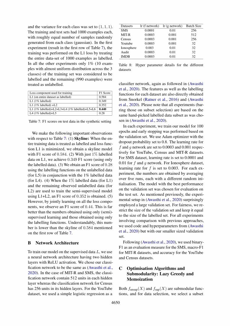
and the variance for each class was set to (1, 1, 1).The training and test sets had 1000 examples each,with roughly equal number of samples randomlygenerated from each class (gaussian). In the firstexperiment (result in the first row of Table 7), thetraining was performed on the L1 loss by treatingthe entire data-set of 1000 examples as labelled.In all the other experiments only 1% (10 exam-ples with almost uniform distribution across the 3classes) of the training set was considered to belabelled and the remaining (990 examples) weretreated as unlabelled.

Loss component used for training F1 ScoreL1 (on entire dataset as labelled) 0.584L1 (1% labelled) 0.349L1 (1% labelled) +L2 0.352L1 (1% labelled)+L2+L3+L4 (1% labelled)+L5+L6 0.440L4 (1% labelled)+L5 0.28

Table 7: F1 scores on test data in the synthetic setting

We make the following important observationswith respect to Table 7: (1) Skyline: When the en-tire training data is treated as labelled and loss func-tion L1 is minimized, we obtain a skyline modelwith F1 score of 0.584. (2) With just 1% labelleddata on L1, we achieve 0.349 F1 score (using onlythe labelled data). (3) We obtain an F1 score of 0.28using the labelling functions on the unlabelled data(for L5) in conjunction with the 1% labelled data(for L4). (4) When the 1% labelled data (for L1)and the remaining observed unlabelled data (forL2) are used to train the semi-supervised modelusing L1+L2, an F1 score of 0.352 is obtained. (5)However, by jointly learning on all the loss compo-nents, we observe an F1 score of 0.44. This is farbetter than the numbers obtained using only (semi)-supervised learning and those obtained using onlythe labelling functions. Understandably, this num-ber is lower than the skyline of 0.584 mentionedon the first row of Table 7.

B Network Architecture

To train our model on the supervised data L, we usea neural network architecture having two hiddenlayers with ReLU activation. We chose our classi-fication network to be the same as (Awasthi et al.,2020). In the case of MIT-R and SMS, the classi-fication network contain 512 units in each hiddenlayer whereas the classification network for Censushas 256 units in its hidden layers. For the YouTubedataset, we used a simple logistic regression as a

Datasets lr (f network) lr (g network) Batch SizeSMS 0.0001 0.01 256MIT-R 0.0003 0.001 512Census 0.0003 0.001 256Youtube 0.0003 0.001 32Ionosphere 0.003 0.01 32Audit 0.0003 0.01 32IMDB 0.0003 0.01 32

Table 8: Hyper parameter details for the differentdatasets

classifier network, again as followed in (Awasthiet al., 2020). The features as well as the labellingfunctions for each dataset are also directly obtainedfrom Snorkel (Ratner et al., 2016) and (Awasthiet al., 2020). Please note that all experiments (bar-ring those on subset selection) are based on thesame hand-picked labelled data subset as was cho-sen in (Awasthi et al., 2020).

In each experiment, we train our model for 100epochs and early stopping was performed based onthe validation set. We use Adam optimizer with thedropout probability set to 0.8. The learning rate forf and g network are set to 0.0003 and 0.001 respec-tively for YouTube, Census and MIT-R datasets.For SMS dataset, learning rate is set to 0.0001 and0.01 for f and g network. For Ionosphere dataset,learning rate for f is set to 0.003. For each ex-periment, the numbers are obtained by averagingover five runs, each with a different random ini-tialisation. The model with the best performanceon the validation set was chosen for evaluation onthe test set. As mentioned previously, the experi-mental setup in (Awasthi et al., 2020) surprisinglyemployed a large validation set. For fairness, we re-strict the size of the validation set and keep it equalto the size of the labelled set. For all experimentsinvolving comparison with previous approaches,we used code and hyperparameters from (Awasthiet al., 2020) but with our smaller sized validationset.

Following (Awasthi et al., 2020), we used binary-F1 as an evaluation measure for the SMS, macro-F1for MIT-R datasets, and accuracy for the YouTubeand Census datasets.

C Optimisation Algorithms andSubmodularity: Lazy Greedy andMemoization

Both funsup(X) and fsup(X) are submodular func-tions, and for data selection, we select a subset

4651

Loss CombinationDatasets

YouTube(Accuracy)

SMS(F1)

MIT-R(F1)

IMDB(F1)

Census(Accuracy)

L1+L2+L3+L4 94.6 93.1 72.5 73.6 82.0L1+L2+L4+L6 92.0 91.9 69.7 73.3 81.3L1+L3+L4+L6 94.4 93.2 29.8 74.4 81.0

L1+L2+L3+L4+L6 94.4 92.3 29.5 64.4 80.9L1+L3+L4+L5+L6 94.6 93.4 73.2 77.1 82.0

L1+L2+L3+L4+L5+L6 94.5 93.0 72.8 76.9 81.9

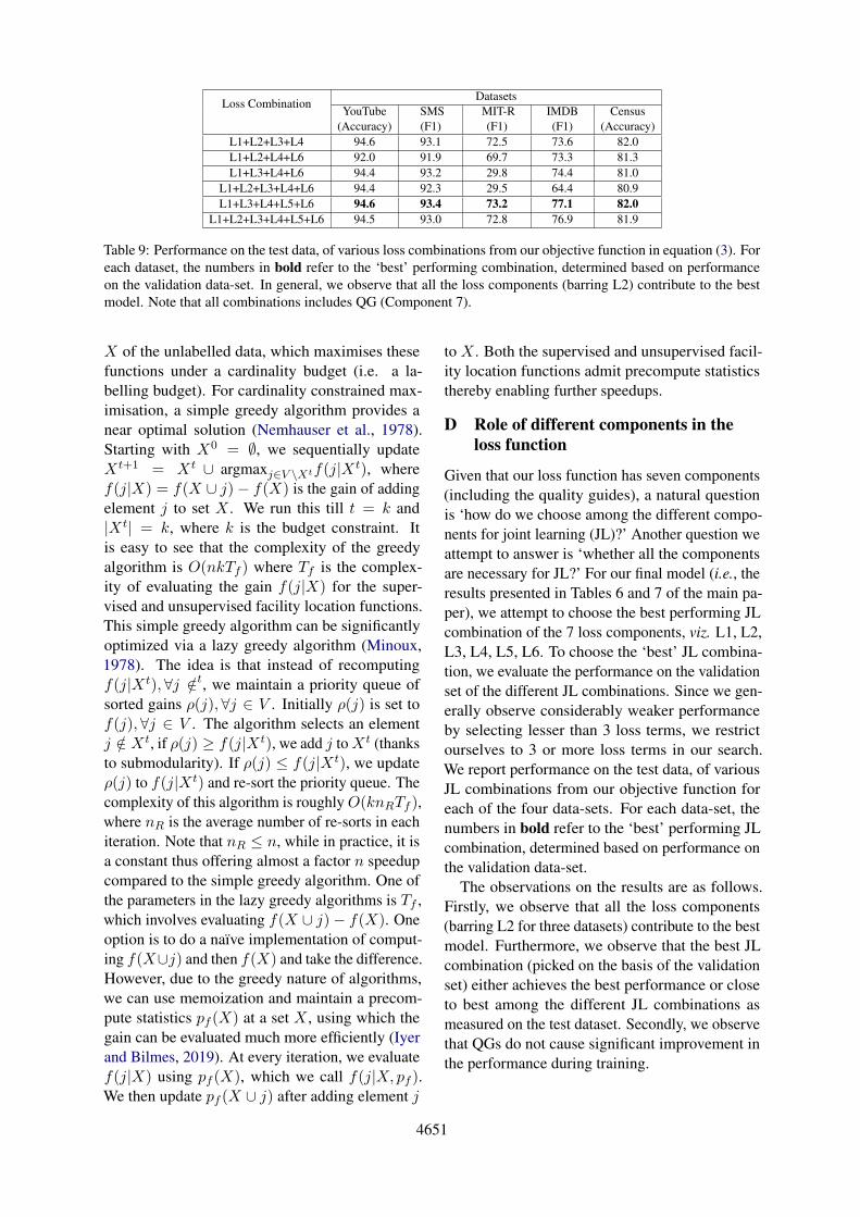
Table 9: Performance on the test data, of various loss combinations from our objective function in equation (3). Foreach dataset, the numbers in bold refer to the ‘best’ performing combination, determined based on performanceon the validation data-set. In general, we observe that all the loss components (barring L2) contribute to the bestmodel. Note that all combinations includes QG (Component 7).

X of the unlabelled data, which maximises thesefunctions under a cardinality budget (i.e. a la-belling budget). For cardinality constrained max-imisation, a simple greedy algorithm provides anear optimal solution (Nemhauser et al., 1978).Starting with X0 = ∅, we sequentially updateXt+1 = Xt ∪ argmaxj∈V \Xtf(j|Xt), wheref(j|X) = f(X ∪ j)− f(X) is the gain of addingelement j to set X . We run this till t = k and|Xt| = k, where k is the budget constraint. Itis easy to see that the complexity of the greedyalgorithm is O(nkTf ) where Tf is the complex-ity of evaluating the gain f(j|X) for the super-vised and unsupervised facility location functions.This simple greedy algorithm can be significantlyoptimized via a lazy greedy algorithm (Minoux,1978). The idea is that instead of recomputingf(j|Xt), ∀j /∈t, we maintain a priority queue ofsorted gains ρ(j),∀j ∈ V . Initially ρ(j) is set tof(j),∀j ∈ V . The algorithm selects an elementj /∈ Xt, if ρ(j) ≥ f(j|Xt), we add j toXt (thanksto submodularity). If ρ(j) ≤ f(j|Xt), we updateρ(j) to f(j|Xt) and re-sort the priority queue. Thecomplexity of this algorithm is roughlyO(knRTf ),where nR is the average number of re-sorts in eachiteration. Note that nR ≤ n, while in practice, it isa constant thus offering almost a factor n speedupcompared to the simple greedy algorithm. One ofthe parameters in the lazy greedy algorithms is Tf ,which involves evaluating f(X ∪ j)− f(X). Oneoption is to do a naıve implementation of comput-ing f(X∪j) and then f(X) and take the difference.However, due to the greedy nature of algorithms,we can use memoization and maintain a precom-pute statistics pf (X) at a set X , using which thegain can be evaluated much more efficiently (Iyerand Bilmes, 2019). At every iteration, we evaluatef(j|X) using pf (X), which we call f(j|X, pf ).We then update pf (X ∪ j) after adding element j

to X . Both the supervised and unsupervised facil-ity location functions admit precompute statisticsthereby enabling further speedups.

D Role of different components in theloss function

Given that our loss function has seven components(including the quality guides), a natural questionis ‘how do we choose among the different compo-nents for joint learning (JL)?’ Another question weattempt to answer is ‘whether all the componentsare necessary for JL?’ For our final model (i.e., theresults presented in Tables 6 and 7 of the main pa-per), we attempt to choose the best performing JLcombination of the 7 loss components, viz. L1, L2,L3, L4, L5, L6. To choose the ‘best’ JL combina-tion, we evaluate the performance on the validationset of the different JL combinations. Since we gen-erally observe considerably weaker performanceby selecting lesser than 3 loss terms, we restrictourselves to 3 or more loss terms in our search.We report performance on the test data, of variousJL combinations from our objective function foreach of the four data-sets. For each data-set, thenumbers in bold refer to the ‘best’ performing JLcombination, determined based on performance onthe validation data-set.

The observations on the results are as follows.Firstly, we observe that all the loss components(barring L2 for three datasets) contribute to the bestmodel. Furthermore, we observe that the best JLcombination (picked on the basis of the validationset) either achieves the best performance or closeto best among the different JL combinations asmeasured on the test dataset. Secondly, we observethat QGs do not cause significant improvement inthe performance during training.